


1 Introduction
The dispersion of pairs of particles remains an active field of research in the study of turbulence. Not only does it continue to hold much theoretical interest, it has important practical applications through the connection between relative dispersion and both concentration fluctuations and mixing.
Simple models of relative dispersion play an important role in understanding the physical processes involved. One such model is a Lagrangian stochastic model (LSM): the central assumption of such models is that the position and velocity of a pair of marked particles can be treated jointly as a continuous Markov process (Thomson Reference Thomson1987; Wilson & Sawford Reference Wilson and Sawford1996). This is a reasonable assumption for the inertial subrange of turbulence. Thomson (Reference Thomson1990) developed an LSM for relative dispersion assuming that the two-point velocity distribution is Gaussian; here we extend it to the non-Gaussian case.
The celebrated Kolmogorov four-fifths law is arguably the simplest manifestation of the non-Gaussian nature of turbulence. It is also one of the few exact results in three-dimensional (3-D) isotropic turbulence and is strongly linked to the cascade of energy from large to small scales. It should therefore be part of any model of turbulent relative dispersion.
A non-zero third-order moment has been incorporated into quasi-one-dimensional (Q1D) models of relative dispersion (Kurbanmuradov Reference Kurbanmuradov1997; Borgas & Yeung Reference Borgas and Yeung2004). These models represent the longitudinal relative velocity,
 $u_{\Vert }$
, of a pair of particles but assume that the transverse velocity component plays no role in the evolution of
 $u_{\Vert }$
and hence no role in the evolution of the distance between the two particles. Pagnini (Reference Pagnini2008) has shown that the longitudinal and transverse velocity components are not statistically independent, which would also be inconsistent with the Navier–Stokes equations. This drawback of Q1D models is the reason these models predict much larger rates of separation than are commonly found experimentally, from direct numerical simulations (DNS) of homogeneous isotropic turbulence or indeed from a Gaussian two-particle LSM such as that of Thomson (Reference Thomson1990).
The limitations of Q1D models have been addressed by the development of quasi-two-dimensional (Q2D) models of relative dispersion (Pagnini Reference Pagnini2008; Sawford & Yeung Reference Sawford and Yeung2010) which include the transverse component of the relative velocity as well as the longitudinal one. These models have successfully shown that the rate of separation is slower compared with Q1D models. However, unlike Q1D models, Q2D models are not unique (even if, as here, we only consider models with position and velocity evolving jointly as a diffusion process with specified random forcing).
In this study we restrict attention to relative dispersion in the inertial subrange of 3-D isotropic turbulence. We also assume that the flow is incompressible and quasi-stationary (with any non-stationarity being on a slow time scale compared to the time scales of interest). In the next section we introduce the LSM and show that, by transforming to spherical polar coordinates, the 3-D model reduces to a Q2D model (if knowledge of the absolute separation is all that is required). We propose an analytical form of the probability density function (p.d.f.) of the Eulerian longitudinal velocity difference that satisfies Kolmogorov’s four-fifths law and use this to derive an analytical form of the model. This model is formulated to have an infinite inertial subrange. The solution of the LSM is investigated numerically for both forwards and backwards dispersion. Finally, in § 6, we consider the differences that occur when the analytical non-Gaussian longitudinal relative velocity p.d.f. is replaced with a numerical one (with a finite inertial subrange) taken from a DNS of relative dispersion.
2 Lagrangian stochastic model
Since we are primarily interested in the relative dispersion statistics, we consider only the relative velocity,
 $\boldsymbol{u}$
, and separation,
 $\boldsymbol{x}$
, of a pair of particles. The evolution of
 $(\boldsymbol{x},\boldsymbol{u})$
is assumed to be governed by
 $$\begin{eqnarray}\left.\begin{array}{@{}c@{}}\text{d}u_{i}=a_{i}(\boldsymbol{x},\boldsymbol{u},t)\,\text{d}t+\sqrt{2C_{0}\unicode[STIX]{x1D700}}\,\text{d}W_{i}(t),\quad i=1,\ldots ,3\\ \text{d}x_{i}=u_{i}\,\text{d}t,\end{array}\right\}\end{eqnarray}$$
where
 $\text{d}\boldsymbol{W}$
is the increment of a vector-valued Wiener process,
 $\unicode[STIX]{x1D700}$
is the mean dissipation rate and
 $C_{0}$
is the constant of proportionality in the second-order Lagrangian velocity structure function. The well-mixed condition (Thomson Reference Thomson1987) constrains the model to be consistent with the Eulerian velocity statistics and leads to an appropriate form for the drift term
 $\boldsymbol{a}$
. In more than one dimension, however, the well-mixed condition does not constrain the drift term uniquely.
For an ensemble of pairs with a given distribution of
 $\boldsymbol{x}$
and
 $\boldsymbol{u}$
at time
 $t^{\prime }$
, the joint p.d.f. of
 $(\boldsymbol{x},\boldsymbol{u})$
at time
 $t$
,
 $p(\boldsymbol{u},\boldsymbol{x},t)$
, satisfies the Fokker–Planck equation corresponding to (2.1):
 $$\begin{eqnarray}\frac{\unicode[STIX]{x2202}p}{\unicode[STIX]{x2202}t}+\frac{\unicode[STIX]{x2202}u_{i}p}{\unicode[STIX]{x2202}x_{i}}+\frac{\unicode[STIX]{x2202}a_{i}p}{\unicode[STIX]{x2202}u_{i}}=C_{0}\unicode[STIX]{x1D700}\frac{\unicode[STIX]{x2202}^{2}p}{\unicode[STIX]{x2202}u_{i}^{2}}.\end{eqnarray}$$
By considering the ensemble of all pairs and noting that, for this ensemble,
 $p(\boldsymbol{u},\boldsymbol{x},t)$
is proportional to the Eulerian relative velocity p.d.f.
 $p_{E}(\boldsymbol{u},\boldsymbol{x},t)$
, it follows that the value of
 $\boldsymbol{a}$
in the model should be such that
 $p_{E}(\boldsymbol{u},\boldsymbol{x},t)$
satisfies (2.2). Following Thomson (Reference Thomson1987, Reference Thomson1990) and Sawford & Yeung (Reference Sawford and Yeung2010), we write
 $\boldsymbol{a}=\boldsymbol{a}^{(1)}+\boldsymbol{a}^{(2)}$
and partition (2.2) for
 $p=p_{E}$
so that
 $$\begin{eqnarray}a_{i}^{(1)}=C_{0}\unicode[STIX]{x1D700}\frac{\unicode[STIX]{x2202}\ln p_{E}}{\unicode[STIX]{x2202}u_{i}}\end{eqnarray}$$
and
 $\boldsymbol{a}^{(2)}$
satisfies
 $$\begin{eqnarray}\frac{\unicode[STIX]{x2202}p_{E}}{\unicode[STIX]{x2202}t}+\frac{\unicode[STIX]{x2202}u_{i}p_{E}}{\unicode[STIX]{x2202}x_{i}}+\frac{\unicode[STIX]{x2202}a_{i}^{(2)}p_{E}}{\unicode[STIX]{x2202}u_{i}}=0.\end{eqnarray}$$
If we write
 $a_{i}^{(2)}=\langle \text{D}u_{i}/\text{D}t|\boldsymbol{u},\boldsymbol{x},t\rangle$
where
 $\text{D}/\text{D}t$
is the material derivative, equation (2.4) is the exact transport equation for
 $p_{E}$
(see e.g. Pope Reference Pope2000, p. 704). (Despite (2.4) not determining
 $\boldsymbol{a}^{(2)}$
uniquely, it is correct to identify
 $\boldsymbol{a}^{(2)}$
with the conditional mean acceleration. This can be seen by noting that, in the (forwards) model and the equivalent backwards model (see Thomson (Reference Thomson1987), § 3.4),
 $\boldsymbol{a}^{(2)}$
is the average of the mean accelerations in the forwards and backwards models for pairs at
 $(\boldsymbol{x},\boldsymbol{u},t)$
, that is, for a well-mixed distribution of pairs,
 $\boldsymbol{a}^{(2)}$
is the average of the model mean accelerations at
 $t-$
and
 $t+$
. However
 $\boldsymbol{a}^{(2)}$
is not the model mean conditional acceleration at
 $t+$
. This is an artefact of the non-differentiability of the velocity in the model.) Specifying either
 $p_{E}$
or
 $\langle Du_{i}/Dt|\boldsymbol{u},\boldsymbol{x},t\rangle$
constrains the form of
 $\boldsymbol{a}(\boldsymbol{x},\boldsymbol{u},t)$
, with
 $\boldsymbol{a}$
uniquely determined in the latter case but not in the former. Here, we will specify the form of
 $p_{E}$
to constrain
 $\boldsymbol{a}$
.
2.1 LSM in spherical polar coordinates
From here on, it is more convenient to work in terms of spherical polar coordinates. The transformation of (2.1) is given by Ito’s formula
 $$\begin{eqnarray}\text{d}f(\tilde{\boldsymbol{x}})=\left(\tilde{a}_{i}\frac{\unicode[STIX]{x2202}f}{\unicode[STIX]{x2202}\tilde{x}_{i}}+\frac{1}{2}(\tilde{\boldsymbol{b}}\tilde{\boldsymbol{b}}^{\text{T}})_{ij}\frac{\unicode[STIX]{x2202}^{2}f}{\unicode[STIX]{x2202}\tilde{x}_{i}\unicode[STIX]{x2202}\tilde{x}_{j}}\right)\text{d}t+\tilde{b}_{ij}\frac{\unicode[STIX]{x2202}f}{\unicode[STIX]{x2202}\tilde{x}_{i}}\,\text{d}W_{j}\quad i,j=1,\ldots ,6\end{eqnarray}$$
for any function
 $f(\tilde{\boldsymbol{x}})$
where
 $\tilde{\boldsymbol{x}}=(x_{1},x_{2},x_{3},u_{1},u_{2},u_{3})$
,
 $\tilde{\boldsymbol{a}}=(u_{1},u_{2},u_{3},a_{1},a_{2},a_{3})$
and
 $\tilde{\boldsymbol{b}}=\sqrt{2C_{0}\unicode[STIX]{x1D700}}\,\text{diag}(0,0,0,1,1,1)$
. Specifying the basis vectors as
 $$\begin{eqnarray}\boldsymbol{e}_{r}=\frac{\boldsymbol{x}}{r},\quad \boldsymbol{e}_{\unicode[STIX]{x1D703}}=\cos \unicode[STIX]{x1D703}\cos \unicode[STIX]{x1D719}\boldsymbol{i}+\cos \unicode[STIX]{x1D703}\sin \unicode[STIX]{x1D719}\boldsymbol{j}-\sin \unicode[STIX]{x1D703}\boldsymbol{k},\quad \boldsymbol{e}_{\unicode[STIX]{x1D719}}=-\!\sin \unicode[STIX]{x1D719}\boldsymbol{i}+\cos \unicode[STIX]{x1D719}\boldsymbol{j},\end{eqnarray}$$
where
 $\unicode[STIX]{x1D703}=\arccos (x_{3}/r)$
and
 $\unicode[STIX]{x1D719}=\arctan (x_{2}/x_{1})$
are the polar and azimuthal angles respectively, we define the components of
 $\boldsymbol{u}$
in spherical polar coordinates as
 $$\begin{eqnarray}u_{\Vert }=\boldsymbol{u}\boldsymbol{\cdot }\boldsymbol{e}_{r},\quad u_{\bot }=\boldsymbol{u}\boldsymbol{\cdot }\boldsymbol{e}_{\unicode[STIX]{x1D703}},\quad u_{\vdash }=\boldsymbol{u}\boldsymbol{\cdot }\boldsymbol{e}_{\unicode[STIX]{x1D719}},\end{eqnarray}$$
where
 $u_{\Vert }$
is the longitudinal component and
 $u_{\bot }$
and
 $u_{\vdash }$
are the transverse components. Using (2.5), we can obtain a stochastic differential equation (SDE) for any function of
 $\tilde{\boldsymbol{x}}$
. The SDEs for
 $u_{\Vert }$
,
 $u_{\bot }$
and
 $u_{\vdash }$
are given by
 $$\begin{eqnarray}\displaystyle & \text{d}u_{\Vert }=a_{\Vert }\text{d}t+\sqrt{2C_{0}\unicode[STIX]{x1D700}}\,\text{d}W_{\Vert }, & \displaystyle\end{eqnarray}$$
 $$\begin{eqnarray}\displaystyle & \text{d}u_{\bot }=a_{\bot }\,\text{d}t+\sqrt{2C_{0}\unicode[STIX]{x1D700}}\,\text{d}W_{\bot }, & \displaystyle\end{eqnarray}$$
and
 $$\begin{eqnarray}\text{d}u_{\vdash }=a_{\vdash }\,\text{d}t+\sqrt{2C_{0}\unicode[STIX]{x1D700}}\,\text{d}W_{\vdash },\end{eqnarray}$$
where
 $$\begin{eqnarray}\displaystyle & \displaystyle a_{\Vert }=\boldsymbol{a}\boldsymbol{\cdot }\boldsymbol{e}_{r}+\boldsymbol{u}\boldsymbol{\cdot }\dot{\boldsymbol{e}}_{r}=\frac{\boldsymbol{a}\boldsymbol{\cdot }\boldsymbol{x}}{r}+\frac{u_{\bot }^{2}+u_{\vdash }^{2}}{r}, & \displaystyle\end{eqnarray}$$
 $$\begin{eqnarray}\displaystyle & \displaystyle a_{\bot }=\boldsymbol{a}\boldsymbol{\cdot }\boldsymbol{e}_{\unicode[STIX]{x1D703}}+\boldsymbol{u}\boldsymbol{\cdot }\dot{\boldsymbol{e}}_{\unicode[STIX]{x1D703}}=\boldsymbol{a}\boldsymbol{\cdot }\boldsymbol{e}_{\unicode[STIX]{x1D703}}+\frac{u_{\vdash }^{2}\cos \unicode[STIX]{x1D703}}{r\sin \unicode[STIX]{x1D703}}-\frac{u_{\Vert }u_{\bot }}{r}, & \displaystyle\end{eqnarray}$$
and
 $$\begin{eqnarray}a_{\vdash }=\boldsymbol{a}\boldsymbol{\cdot }\boldsymbol{e}_{\unicode[STIX]{x1D719}}+\boldsymbol{u}\boldsymbol{\cdot }\dot{\boldsymbol{e}}_{\unicode[STIX]{x1D719}}=\boldsymbol{a}\boldsymbol{\cdot }\boldsymbol{e}_{\unicode[STIX]{x1D719}}-\frac{u_{\Vert }u_{\vdash }}{r}-\frac{u_{\bot }u_{\vdash }\cos \unicode[STIX]{x1D703}}{r\sin \unicode[STIX]{x1D703}},\end{eqnarray}$$
with
 $\text{d}W_{\Vert }=\text{d}\boldsymbol{W}\boldsymbol{\cdot }\boldsymbol{e}_{r}$
,
 $\text{d}W_{\bot }=\text{d}\boldsymbol{W}\boldsymbol{\cdot }\boldsymbol{e}_{\unicode[STIX]{x1D703}}$
and
 $\text{d}W_{\vdash }=\text{d}\boldsymbol{W}\boldsymbol{\cdot }\boldsymbol{e}_{\unicode[STIX]{x1D719}}$
. We see that
 $a_{\Vert }$
,
 $a_{\bot }$
and
 $a_{\vdash }$
are equal to the component of
 $\boldsymbol{a}$
in the relevant direction plus a ‘metric’ term arising from the curved coordinate system. The SDE for the absolute perpendicular velocity,
 $u_{p}=\sqrt{u_{\bot }^{2}+u_{\vdash }^{2}}$
, is given by
 $$\begin{eqnarray}\text{d}u_{p}=a_{p}\,\text{d}t+\sqrt{2C_{0}\unicode[STIX]{x1D700}}\,\text{d}W_{p},\end{eqnarray}$$
where
 $$\begin{eqnarray}a_{p}=\boldsymbol{a}\boldsymbol{\cdot }\frac{\boldsymbol{u}-u_{\Vert }\boldsymbol{x}/r}{u_{p}}+\frac{C_{0}\unicode[STIX]{x1D700}}{u_{p}}-\frac{u_{\Vert }u_{p}}{r}\end{eqnarray}$$
and
 $\text{d}W_{p}=\text{d}\boldsymbol{W}\boldsymbol{\cdot }(\boldsymbol{u}-u_{\Vert }\boldsymbol{x}/r)/u_{p}$
. The SDEs for
 $r$
,
 $\unicode[STIX]{x1D703}$
and
 $\unicode[STIX]{x1D719}$
are simply
 $\text{d}r=u_{\Vert }\,\text{d}t$
,
 $\text{d}\unicode[STIX]{x1D703}=(u_{\bot }/r)\,\text{d}t$
and
 $\text{d}\unicode[STIX]{x1D719}=(u_{\vdash }/r\sin \unicode[STIX]{x1D703})\,\text{d}t$
. Because of our assumption of isotropy,
 $p_{E}$
depends only on
 $u_{\Vert }$
,
 $u_{p}$
and
 $r$
and, to ensure
 $\boldsymbol{a}$
is consistent with our assumption of isotropy,
 $a_{\Vert }$
and
 $a_{p}$
must be chosen to depend only on
 $u_{\Vert }$
,
 $u_{p}$
and
 $r$
. Thus, in isotropic turbulence, equations (2.8), (2.14) and
 $\text{d}r=u_{\Vert }\,\text{d}t$
are sufficient for determining the relative dispersion statistics. In effect, the 3-D model has been reduced to a Q2D model.
The Fokker–Planck equation corresponding to (2.8)–(2.10) and the equations for
 $\text{d}r$
,
 $\text{d}\unicode[STIX]{x1D703}$
and
 $\text{d}\unicode[STIX]{x1D719}$
is
 $$\begin{eqnarray}\frac{\unicode[STIX]{x2202}\hat{p}}{\unicode[STIX]{x2202}t}+\frac{\unicode[STIX]{x2202}u_{\Vert }\hat{p}}{\unicode[STIX]{x2202}r}+\frac{\unicode[STIX]{x2202}(u_{\bot }/r)\hat{p}}{\unicode[STIX]{x2202}\unicode[STIX]{x1D703}}+\frac{\unicode[STIX]{x2202}(u_{\vdash }/r\sin \unicode[STIX]{x1D703})\hat{p}}{\unicode[STIX]{x2202}\unicode[STIX]{x1D719}}+\frac{\unicode[STIX]{x2202}a_{\Vert }\hat{p}}{\unicode[STIX]{x2202}u_{\Vert }}+\frac{\unicode[STIX]{x2202}a_{\bot }\hat{p}}{\unicode[STIX]{x2202}u_{\bot }}+\frac{\unicode[STIX]{x2202}a_{\vdash }\hat{p}}{\unicode[STIX]{x2202}u_{\vdash }}=C_{0}\unicode[STIX]{x1D700}\unicode[STIX]{x1D6FB}_{\boldsymbol{u}}^{2}\hat{p}.\quad\end{eqnarray}$$
Here
 $\hat{p}$
is the density function of the distribution of all pairs in
 $(r,\unicode[STIX]{x1D703},\unicode[STIX]{x1D719},u_{\Vert },u_{\bot },u_{\vdash })$
-space and equals
 $r^{2}\sin \unicode[STIX]{x1D703}\,p(\boldsymbol{u},\boldsymbol{x},t)$
, with
 $r^{2}\sin \unicode[STIX]{x1D703}$
being the Jacobian of the transformation between the two coordinate systems, while
 $\unicode[STIX]{x1D6FB}_{\boldsymbol{u}}^{2}$
denotes
 $\unicode[STIX]{x2202}^{2}/\unicode[STIX]{x2202}u_{\Vert }^{2}+\unicode[STIX]{x2202}^{2}/\unicode[STIX]{x2202}u_{\bot }^{2}+\unicode[STIX]{x2202}^{2}/\unicode[STIX]{x2202}u_{\vdash }^{2}$
. This can also be derived by transforming (2.2) to the new coordinate system (Risken Reference Risken1989, pp. 88–91). Note that, if we regard the
 $(x_{1},x_{2},x_{3},u_{1},u_{2},u_{3})$
-coordinate system as orthogonal, then the
 $(r,\unicode[STIX]{x1D703},\unicode[STIX]{x1D719},u_{\Vert },u_{\bot },u_{\vdash })$
-coordinate system is non-orthogonal. This is because if we consider a vector along a trajectory with either
 $\unicode[STIX]{x1D703}$
or
 $\unicode[STIX]{x1D719}$
changing and with the remaining coordinates in the
 $(r,\unicode[STIX]{x1D703},\unicode[STIX]{x1D719},u_{\Vert },u_{\bot },u_{\vdash })$
-coordinate system held constant (i.e. what one might call a vector in the
 $\unicode[STIX]{x1D703}$
or
 $\unicode[STIX]{x1D719}$
direction), then this vector has components in some of the
 $(u_{1},u_{2},u_{3})$
directions as well as in the
 $(x_{1},x_{2},x_{3})$
directions (i.e.
 $(u_{1},u_{2},u_{3})$
changes along the trajectory). Hence we cannot use results for orthogonal coordinate systems to make the transformation. As with (2.2), the model should be such that (2.16) is satisfied by
 $\hat{p}_{E}=r^{2}\sin \unicode[STIX]{x1D703}p_{E}$
. Because of isotropy,
 $p_{E}$
has no dependence on
 $\unicode[STIX]{x1D703}$
and
 $\unicode[STIX]{x1D719}$
(for fixed
 $r$
,
 $u_{\Vert }$
,
 $u_{\bot }$
and
 $u_{\vdash }$
) and so, for stationary turbulence, we obtain
 $$\begin{eqnarray}\frac{\unicode[STIX]{x2202}u_{\Vert }\hat{p}_{E}}{\unicode[STIX]{x2202}r}+\frac{u_{\bot }\hat{p}_{E}\cos \unicode[STIX]{x1D703}}{r\sin \unicode[STIX]{x1D703}}+\frac{\unicode[STIX]{x2202}a_{\Vert }\hat{p}_{E}}{\unicode[STIX]{x2202}u_{\Vert }}+\frac{\unicode[STIX]{x2202}a_{\bot }\hat{p}_{E}}{\unicode[STIX]{x2202}u_{\bot }}+\frac{\unicode[STIX]{x2202}a_{\vdash }\hat{p}_{E}}{\unicode[STIX]{x2202}u_{\vdash }}=C_{0}\unicode[STIX]{x1D700}\unicode[STIX]{x1D6FB}_{\boldsymbol{u}}^{2}\hat{p}_{E}.\end{eqnarray}$$
It is convenient, in our new coordinate system, to follow the split
 $\boldsymbol{a}=\boldsymbol{a}^{(1)}+\boldsymbol{a}^{(2)}$
introduced above and to split
 $a_{\Vert }$
,
 $a_{\bot }$
and
 $a_{\vdash }$
into (i) terms proportional to
 $C_{0}$
which balance the right-hand side of (2.17), (ii) metric terms arising from
 $\dot{\boldsymbol{e}}_{r}$
,
 $\dot{\boldsymbol{e}}_{\unicode[STIX]{x1D703}}$
and
 $\dot{\boldsymbol{e}}_{\unicode[STIX]{x1D719}}$
and (iii) terms related to the conditional mean accelerations (the metric terms have no equivalent in the Cartesian coordinate system used above), giving
 $$\begin{eqnarray}\displaystyle & \displaystyle a_{\Vert }=C_{0}\unicode[STIX]{x1D700}\frac{\unicode[STIX]{x2202}\ln p_{E}}{\unicode[STIX]{x2202}u_{\Vert }}+\frac{u_{\bot }^{2}+u_{\vdash }^{2}}{r}+a_{\Vert }^{\prime }, & \displaystyle\end{eqnarray}$$
 $$\begin{eqnarray}\displaystyle & \displaystyle a_{\bot }=C_{0}\unicode[STIX]{x1D700}\frac{\unicode[STIX]{x2202}\ln p_{E}}{\unicode[STIX]{x2202}u_{\bot }}+\frac{u_{\vdash }^{2}\cos \unicode[STIX]{x1D703}}{r\sin \unicode[STIX]{x1D703}}-\frac{u_{\Vert }u_{\bot }}{r}+a_{\bot }^{\prime } & \displaystyle\end{eqnarray}$$
and
 $$\begin{eqnarray}a_{\vdash }=C_{0}\unicode[STIX]{x1D700}\frac{\unicode[STIX]{x2202}\ln p_{E}}{\unicode[STIX]{x2202}u_{\vdash }}-\frac{u_{\Vert }u_{\vdash }}{r}-\frac{u_{\bot }u_{\vdash }\cos \unicode[STIX]{x1D703}}{r\sin \unicode[STIX]{x1D703}}+a_{\vdash }^{\prime }.\end{eqnarray}$$
Conceptually, in Cartesian coordinates,
 $\boldsymbol{a}$
is both the conditional mean acceleration vector in the immediate future and the deterministic term in the SDE, with
 $\boldsymbol{a}^{(2)}$
corresponding to the conditional mean acceleration at the current time and
 $\boldsymbol{a}^{(1)}$
being the difference between that and the conditional mean acceleration in the immediate future. In the non-Cartesian coordinates, the conditional mean acceleration vector in the immediate future and the deterministic term in the SDE are no longer equal, with the metric terms reflecting this difference, and with the
 $C_{0}$
terms and
 $(a_{\Vert }^{\prime },a_{\bot }^{\prime },a_{\vdash }^{\prime })$
being the vectors
 $\boldsymbol{a}^{(1)}$
and
 $\boldsymbol{a}^{(2)}$
re-expressed in terms of
 $\boldsymbol{e}_{r}$
,
 $\boldsymbol{e}_{\unicode[STIX]{x1D703}}$
and
 $\boldsymbol{e}_{\unicode[STIX]{x1D719}}$
.
Because of isotropy,
 $p_{E}$
and
 $a_{\Vert }^{\prime }$
must depend only on
 $u_{\Vert }$
,
 $u_{p}$
and
 $r$
(as noted above). Isotropy also implies that
 $(a_{\bot }^{\prime },a_{\vdash }^{\prime })=(u_{\bot },u_{\vdash }){\mathcal{A}}^{\prime }$
for some
 ${\mathcal{A}}^{\prime }$
(since
 $(u_{\bot },u_{\vdash })$
defines the only possible direction for
 $(a_{\bot }^{\prime },a_{\vdash }^{\prime })$
) with
 ${\mathcal{A}}^{\prime }$
depending only on
 $u_{\Vert }$
,
 $u_{p}$
and
 $r$
. We note that
 ${\mathcal{A}}^{\prime }=a_{p}^{\prime }/u_{p}$
where
 $a_{p}^{\prime }$
is the non-
 $C_{0}$
and non-metric part of
 $a_{p}$
. It follows that
 $a_{\Vert }^{\prime }$
and
 ${\mathcal{A}}^{\prime }$
should satisfy
 $$\begin{eqnarray}\frac{\unicode[STIX]{x2202}u_{\Vert }r^{2}u_{p}p_{E}}{\unicode[STIX]{x2202}r}+\frac{\unicode[STIX]{x2202}}{\unicode[STIX]{x2202}u_{\Vert }}\left(a_{\Vert }^{\prime }+\frac{u_{p}^{2}}{r}\right)r^{2}u_{p}p_{E}+\frac{\unicode[STIX]{x2202}}{\unicode[STIX]{x2202}u_{p}}u_{p}\left({\mathcal{A}}^{\prime }-\frac{u_{\Vert }}{r}\right)r^{2}u_{p}p_{E}=0\end{eqnarray}$$
(here
 $r^{2}u_{p}p_{E}$
is the density function of the well-mixed distribution in
 $(r,u_{\Vert },u_{p})$
-space).
Our approach to designing the model is to choose a form for
 $p_{E}$
and then select
 $a_{\Vert }^{\prime }$
and
 ${\mathcal{A}}^{\prime }$
to be consistent with (2.21). We can choose either
 ${\mathcal{A}}^{\prime }$
or
 $a_{\Vert }^{\prime }$
and then calculate the other quantity by integrating (2.21). We assume that
 $p_{E}$
is well behaved in the sense of tending to zero sufficiently rapidly as
 $u_{\Vert }$
or
 $u_{p}\rightarrow \infty$
and remaining bounded as
 $u_{p}\rightarrow 0$
. We also assume that the chosen value of
 $a_{\Vert }^{\prime }$
(or of
 ${\mathcal{A}}^{\prime }$
) gives zero fluxes at infinite velocity (and, for
 ${\mathcal{A}}^{\prime }$
, across the boundary at
 $u_{p}=0$
). However this also needs to be true for the calculated quantities, that is, if
 $a_{\Vert }^{\prime }$
is calculated, we require that
 $a_{\Vert }^{\prime }p_{E}$
tends to zero at both
 $u_{\Vert }=-\infty$
and
 $u_{\Vert }=\infty$
while, if
 ${\mathcal{A}}^{\prime }$
is calculated, we require that
 $u_{p}^{2}{\mathcal{A}}^{\prime }p_{E}$
tends to zero at both
 $u_{p}=0$
and
 $u_{p}=\infty$
. One of these limits can be satisfied by adjusting the constant of integration, but satisfying both limits imposes a restriction on the initial choice of
 ${\mathcal{A}}^{\prime }$
(or
 $a_{\Vert }^{\prime }$
).
 ${\mathcal{A}}^{\prime }$
needs to satisfy
 $$\begin{eqnarray}\frac{\unicode[STIX]{x2202}}{\unicode[STIX]{x2202}r}\int _{-\infty }^{\infty }u_{\Vert }r^{2}u_{p}p_{E}\,\text{d}u_{\Vert }+\frac{\unicode[STIX]{x2202}}{\unicode[STIX]{x2202}u_{p}}\int _{-\infty }^{\infty }u_{p}\left({\mathcal{A}}^{\prime }-\frac{u_{\Vert }}{r}\right)r^{2}u_{p}p_{E}\,\text{d}u_{\Vert }=0,\end{eqnarray}$$
while
 $a_{\Vert }^{\prime }$
needs to satisfy
 $$\begin{eqnarray}\frac{\unicode[STIX]{x2202}}{\unicode[STIX]{x2202}r}\int _{0}^{\infty }u_{\Vert }r^{2}u_{p}p_{E}\,\text{d}u_{p}+\frac{\unicode[STIX]{x2202}}{\unicode[STIX]{x2202}u_{\Vert }}\int _{0}^{\infty }\left(a_{\Vert }^{\prime }+\frac{u_{p}^{2}}{r}\right)r^{2}u_{p}p_{E}\,\text{d}u_{p}=0.\end{eqnarray}$$
We note that the second of these constraints amounts to saying that the model must satisfy the well-mixed condition for a Q1D model when averaged over
 $u_{p}$
.
2.2 The Eulerian p.d.f.
 $p_{E}$
and the model functions
$a_{\Vert }^{\prime }$
and
${\mathcal{A}}^{\prime }$


There is considerable freedom in designing the model, both in the choice of
 $p_{E}$
and the choice of
 $a_{\Vert }^{\prime }$
and
 ${\mathcal{A}}^{\prime }$
. Although these choices could be based on experimental data, as investigated by Sawford & Yeung (Reference Sawford and Yeung2010), our main aim here is to investigate the usefulness of relatively simple idealised model formulations. We discuss a range of idealisations, including cases where
 $p_{E}$
is separable, either in terms of
 $u_{\Vert }$
and
 $u_{p}$
or in terms of
 $u_{\Vert }$
,
 $u_{\bot }$
and
 $u_{\vdash }$
; cases with Gaussian velocity distributions, either just for
 $u_{\bot }$
and
 $u_{\vdash }$
or for
 $u_{\Vert }$
,
 $u_{\bot }$
and
 $u_{\vdash }$
; cases where
 $a_{\bot }^{\prime }$
and
 $a_{\vdash }^{\prime }$
are quadratic functions of velocity; and cases where the model reduces to a Q1D model. We then describe a particular set of choices to be used for the model simulations presented below.
A natural simplification is to assume that
 $p_{E}$
is separable in
 $u_{\Vert }$
and
 $u_{p}$
and can be written as
 $$\begin{eqnarray}p_{E}(u_{\Vert },u_{\bot },u_{\vdash })=\frac{p_{u_{\Vert }}(u_{\Vert })p_{u_{p}}(u_{p})}{2\unicode[STIX]{x03C0}u_{p}}.\end{eqnarray}$$
A consequence of this assumption is that any dependence of the transverse and longitudinal velocity components on each other that may exist in reality cannot be taken into account. This cannot be an exact assumption because it implies that the fixed-point moment
 $\langle u_{\Vert }u_{p}^{2}\rangle$
is zero, while, in the inertial subrange, Kolmogorov’s four-fifths law
 $\langle u_{\Vert }^{3}\rangle =-(4/5)\unicode[STIX]{x1D700}r$
combined with incompressibility implies otherwise (Pagnini Reference Pagnini2008, p. 365). In addition, evidence from DNS indicates that the p.d.f. of
 $u_{p}$
conditional on
 $u_{\Vert }$
depends strongly on
 $u_{\Vert }$
(Sawford & Yeung Reference Sawford and Yeung2010). These results imply that
 $p_{E}(\boldsymbol{u})$
is not separable. However, we assume (2.24) in order to make the model tractable; it will be of interest to see how well the model performs despite this limitation. A consequence of this assumption is that because
 $\langle \boldsymbol{u}\boldsymbol{\cdot }\text{D}\boldsymbol{u}/\text{D}t\rangle =3(\langle u_{\Vert }^{3}\rangle +\langle u_{\Vert }u_{p}^{2}\rangle )/(2r)$
in the inertial subrange of turbulence (for both reality and LSMs of the type considered here), our model cannot satisfy both the four-fifths law and the result that in the inertial subrange
 $\langle \boldsymbol{u}\boldsymbol{\cdot }\text{D}\boldsymbol{u}/\text{D}t\rangle =-2\unicode[STIX]{x1D700}$
(Mann, Ott & Andersen Reference Mann, Ott and Andersen1999).
A further possible assumption is that the p.d.f. of
 $(u_{\bot },u_{\vdash })$
is separable with
 $u_{\bot }$
and
 $u_{\vdash }$
being independent:
 $$\begin{eqnarray}p_{u_{p}}(u_{p})=2\unicode[STIX]{x03C0}u_{p}p_{u_{\bot }}(u_{\bot })p_{u_{\vdash }}(u_{\vdash }).\end{eqnarray}$$
Because of isotropy and the circular symmetry of
 $u_{\bot }$
and
 $u_{\vdash }$
, a consequence of the assumption that
 $u_{\bot }$
and
 $u_{\vdash }$
are independent is that
 $p_{u_{\bot }}$
and
 $p_{u_{\vdash }}$
are Gaussian (e.g. Papoulis Reference Papoulis1991, p. 134). It is, of course, equivalent to assume directly that
 $p_{u_{\bot }}$
and
 $p_{u_{\vdash }}$
are Gaussian. We denote the common variance of
 $u_{\bot }$
and
 $u_{\vdash }$
by
 $\unicode[STIX]{x1D70E}_{\bot }^{2}$
.
Even once
 $p_{E}$
is specified, there is still a lot of freedom in choosing
 $a_{\Vert }^{\prime }$
and
 ${\mathcal{A}}^{\prime }$
. We consider choices where the transverse terms
 $a_{\bot }^{\prime }$
and
 $a_{\vdash }^{\prime }$
are quadratic in the velocity components. This implies
 ${\mathcal{A}}^{\prime }$
is equal to
 $u_{\Vert }$
times a function of
 $r$
i.e.
 $$\begin{eqnarray}(a_{\bot }^{\prime },a_{\vdash }^{\prime })=(u_{\bot },u_{\vdash }){\mathcal{A}}^{\prime }=(u_{\bot },u_{\vdash })u_{\Vert }\unicode[STIX]{x1D719}(r)\end{eqnarray}$$
(although, as for the Gaussian case, this still does not imply a unique model, with
 $\unicode[STIX]{x1D719}$
still to be determined). This choice is often made in models where
 $p_{E}$
is assumed to be Gaussian (Thomson Reference Thomson1987; Borgas & Sawford Reference Borgas and Sawford1994). It includes a broad class of Q1D models (see discussion below), and is, when combined with the
 $(u_{\Vert },u_{p})$
-separability assumption, a convenient way of ensuring that (2.22) is satisfied. When (2.26) is combined with the
 $(u_{\Vert },u_{p})$
-separability assumption, equation (2.21) implies
 $$\begin{eqnarray}a_{\Vert }^{\prime }=-\frac{u_{p}^{2}}{r}-\frac{1}{p_{u_{\Vert }}}\left(\frac{\unicode[STIX]{x2202}\ln \tilde{p}_{u_{p}}}{\unicode[STIX]{x2202}r}+\frac{\unicode[STIX]{x2202}}{\unicode[STIX]{x2202}r}+2\unicode[STIX]{x1D719}(r)+u_{p}\left(\unicode[STIX]{x1D719}(r)-\frac{1}{r}\right)\frac{\unicode[STIX]{x2202}\ln \tilde{p}_{u_{p}}}{\unicode[STIX]{x2202}u_{p}}\right)\int _{-\infty }^{u_{\Vert }}u_{\Vert }^{\prime }p_{u_{\Vert }}(u_{\Vert }^{\prime })\,\text{d}u_{\Vert }^{\prime },\end{eqnarray}$$
where
 $\tilde{p}_{u_{p}}=p_{u_{p}}/2\unicode[STIX]{x03C0}u_{p}$
and we have used the condition that the flux
 $a_{\Vert }^{\prime }p_{u_{\Vert }}$
must tend to zero as
 $u_{\Vert }\rightarrow -\infty$
. Note that, if we had chosen
 $a_{\bot }^{\prime }$
or
 $a_{\vdash }^{\prime }$
to contain a term which is linear in the velocity components, then
 ${\mathcal{A}}^{\prime }$
would have a term which is a function of
 $r$
only, which would give rise to a term in
 $a_{\Vert }^{\prime }$
that increases rapidly as
 $u_{\Vert }\rightarrow \infty$
with the flux
 $a_{\Vert }^{\prime }p_{u_{\Vert }}$
not tending to zero in this limit. Also, because
 $(a_{\bot }^{\prime },a_{\vdash }^{\prime })=(u_{\bot },u_{\vdash }){\mathcal{A}}^{\prime }$
, it is impossible to include a constant term in
 $a_{\bot }^{\prime }$
or
 $a_{\vdash }^{\prime }$
. We remark that, with the choice (2.26) and with
 $a_{\Vert }^{\prime }p_{u_{\Vert }}\rightarrow 0$
as
 $u_{\Vert }\rightarrow -\infty$
, the flux also tends to zero as
 $u_{\Vert }\rightarrow \infty$
. If we had chosen to assume
 $a_{\Vert }^{\prime }p_{u_{\Vert }}\rightarrow 0$
as
 $u_{\Vert }\rightarrow \infty$
, then the integral on the right-hand side of (2.27) would be replaced by
 $-\!\int _{u_{\Vert }}^{\infty }$
. This is equivalent because
 $p_{u_{\Vert }}$
has mean zero.
In the case of Gaussian transverse velocity components, or equivalently with the assumption of
 $(u_{\Vert },u_{\bot },u_{\vdash })$
-separability, equation (2.27) becomes
 $$\begin{eqnarray}a_{\Vert }^{\prime }=-\frac{u_{p}^{2}}{r}-\frac{1}{p_{u_{\Vert }}}\left(\frac{\unicode[STIX]{x2202}}{\unicode[STIX]{x2202}r}+\frac{u_{p}^{2}}{\unicode[STIX]{x1D70E}_{\bot }^{2}r}+\left(\unicode[STIX]{x1D719}(r)-\frac{1}{2\unicode[STIX]{x1D70E}_{\bot }^{2}}\frac{\text{d}\unicode[STIX]{x1D70E}_{\bot }^{2}}{\text{d}r}\right)\left(2-\frac{u_{p}^{2}}{\unicode[STIX]{x1D70E}_{\bot }^{2}}\right)\right)\int _{-\infty }^{u_{\Vert }}u_{\Vert }^{\prime }p_{u_{\Vert }}(u_{\Vert }^{\prime })\,\text{d}u_{\Vert }^{\prime }.\end{eqnarray}$$
If we further assume that
 $p_{u_{\Vert }}$
is Gaussian with variance
 $\unicode[STIX]{x1D70E}_{\Vert }^{2}$
, equation (2.28) becomes
 $$\begin{eqnarray}a_{\Vert }^{\prime }=-\frac{u_{p}^{2}}{r}\left(\frac{\unicode[STIX]{x1D70E}_{\bot }^{2}-\unicode[STIX]{x1D70E}_{\Vert }^{2}}{\unicode[STIX]{x1D70E}_{\bot }^{2}}\right)+\frac{\text{d}\unicode[STIX]{x1D70E}_{\Vert }}{\text{d}r}\frac{(\unicode[STIX]{x1D70E}_{\Vert }^{2}+u_{\Vert }^{2})}{\unicode[STIX]{x1D70E}_{\Vert }}+\left(\unicode[STIX]{x1D719}(r)-\frac{1}{2\unicode[STIX]{x1D70E}_{\bot }^{2}}\frac{\text{d}\unicode[STIX]{x1D70E}_{\bot }^{2}}{\text{d}r}\right)\unicode[STIX]{x1D70E}_{\Vert }^{2}\left(2-\frac{u_{p}^{2}}{\unicode[STIX]{x1D70E}_{\bot }^{2}}\right).\end{eqnarray}$$
In this case, the model of Thomson (Reference Thomson1990) corresponds to
 $$\begin{eqnarray}\unicode[STIX]{x1D719}(r)=-\frac{\unicode[STIX]{x1D70E}_{\bot }^{2}-\unicode[STIX]{x1D70E}_{\Vert }^{2}}{2\unicode[STIX]{x1D70E}_{\Vert }^{2}r}+\frac{1}{2\unicode[STIX]{x1D70E}_{\bot }^{2}}\frac{\text{d}\unicode[STIX]{x1D70E}_{\bot }^{2}}{\text{d}r}=-\frac{1}{2\unicode[STIX]{x1D70E}_{\Vert }}\frac{\text{d}\unicode[STIX]{x1D70E}_{\Vert }}{\text{d}r}+\frac{1}{2\unicode[STIX]{x1D70E}_{\bot }^{2}}\frac{\text{d}\unicode[STIX]{x1D70E}_{\bot }^{2}}{\text{d}r},\end{eqnarray}$$
where the last equality is a consequence of incompressibility. This form of
 $\unicode[STIX]{x1D719}(r)$
also ensures that
 $a_{\bot }^{\prime }$
and
 $a_{\vdash }^{\prime }$
agree with Thomson (Reference Thomson1990) regardless of whether the model is Gaussian or not. We note that the form of
 $\unicode[STIX]{x1D719}(r)$
that corresponds to the model of Borgas (Sawford & Guest Reference Sawford and Guest1988; Borgas & Sawford Reference Borgas and Sawford1994, equation (4.2a)) is given by
 $$\begin{eqnarray}\unicode[STIX]{x1D719}(r)=-\frac{\unicode[STIX]{x1D70E}_{\bot }^{2}-\unicode[STIX]{x1D70E}_{\Vert }^{2}}{\unicode[STIX]{x1D70E}_{\Vert }^{2}r}=-\frac{1}{\unicode[STIX]{x1D70E}_{\Vert }}\frac{\text{d}\unicode[STIX]{x1D70E}_{\Vert }}{\text{d}r}.\end{eqnarray}$$
For the
 $(u_{\Vert },u_{\bot },u_{\vdash })$
-separable case, and also for the
 $(u_{\Vert },u_{p})$
-separable case with the restriction that the shape of
 $p_{u_{p}}$
is independent of
 $r$
, we note that, with the quadratic assumption (2.26) and the choice
 $$\begin{eqnarray}\unicode[STIX]{x1D719}(r)=\frac{1}{2\unicode[STIX]{x1D70E}_{\bot }^{2}}\frac{\text{d}\unicode[STIX]{x1D70E}_{\bot }^{2}}{\text{d}r}+\frac{1}{r},\end{eqnarray}$$
we have
 $$\begin{eqnarray}a_{\Vert }^{\prime }=-\frac{u_{p}^{2}}{r}-\frac{1}{p_{u_{\Vert }}}\left(\frac{\unicode[STIX]{x2202}}{\unicode[STIX]{x2202}r}+\frac{2}{r}\right)\int _{-\infty }^{u_{\Vert }}u_{\Vert }^{\prime }p_{u_{\Vert }}(u_{\Vert }^{\prime })\,\text{d}u_{\Vert }^{\prime }\end{eqnarray}$$
(from (2.28) or (2.27)). In the case where
 $p_{u_{\Vert }}$
is Gaussian, we then have
 $$\begin{eqnarray}a_{\Vert }^{\prime }=-\frac{u_{p}^{2}}{r}+\frac{\text{d}\unicode[STIX]{x1D70E}_{\Vert }}{\text{d}r}\frac{(\unicode[STIX]{x1D70E}_{\Vert }^{2}+u_{\Vert }^{2})}{\unicode[STIX]{x1D70E}_{\Vert }}+\frac{2\unicode[STIX]{x1D70E}_{\Vert }^{2}}{r}\end{eqnarray}$$
(from (2.29)). It follows that, for these cases,
 $a_{\Vert }$
does not depend on
 $u_{p}$
. In effect, the separation process has become one-dimensional. Indeed, in this case the model reduces to the Q1D model of Kurbanmuradov (Reference Kurbanmuradov1997, equations (3.1), (4.7) and (4.8)). It can be shown that, provided
 $p_{E}$
is separable in
 $u_{\Vert }$
and
 $u_{p}$
, then, for Q1D models, the quadratic assumption (2.26) holds if and only if the shape of
 $p_{u_{p}}(u_{p})$
is independent of
 $r$
, and in such cases (2.32) is satisfied. The Q1D model is known to overestimate the growth rate of an ensemble of particle pairs in the inertial subrange of homogeneous isotropic turbulence (Kurbanmuradov Reference Kurbanmuradov1997; Sawford & Yeung Reference Sawford and Yeung2010; Devenish & Thomson Reference Devenish and Thomson2011) and, along with the limitations of Q1D models discussed in § 1, suggests (2.32) is not an appropriate choice for formulating quantitatively realistic LSMs.
We note that, for models based on (2.25) and (2.26) in the classical self-similar inertial subrange, we have
 $\unicode[STIX]{x1D719}(r)=\hat{\unicode[STIX]{x1D719}}/r$
for some constant
 $\hat{\unicode[STIX]{x1D719}}$
. Together with
 $p_{u_{\Vert }}$
and
 $C_{0}$
, the value of
 $\hat{\unicode[STIX]{x1D719}}$
characterises the model and is equal to
 $-1/3$
,
 $1/6$
and
 $4/3$
for the Borgas, Thomson and Q1D models respectively.
2.3 Model formulation
We now describe the model configuration chosen for our numerical simulations. We assume
 $(u_{\Vert },u_{\bot },u_{\vdash })$
-separability of
 $p_{E}$
with the quadratic assumption (2.26) and we choose
 $\unicode[STIX]{x1D719}(r)$
to take the form given in (2.30) so that the non-Gaussian model reduces to that of Thomson (Reference Thomson1990) in the case that
 $p_{u_{\Vert }}$
is Gaussian. This avoids the Q1D assumption and allows us to include the important skewness in the longitudinal velocity distribution, while providing a modelling framework without too many remaining degrees of freedom (
 $p_{u_{\Vert }}$
remains to be specified). The
 $(u_{\Vert },u_{p})$
-separability of
 $p_{E}$
is probably the weakest assumption here as this is known not to be exact.
The approach we follow in constructing an analytical form for
 $p_{u_{\Vert }}$
is that developed for modelling single-particle dispersion in the convective atmospheric boundary layer. For the convective atmospheric boundary layer the p.d.f. is positively skewed, i.e. there is a relatively low probability of strong updraughts versus a high probability of weak downdraughts, while for our application
 $p_{u_{\Vert }}$
is negatively skewed. Following Baerentsen & Berkowicz (Reference Baerentsen and Berkowicz1984), Luhar & Britter (Reference Luhar and Britter1989) and Hudson & Thomson (Reference Hudson and Thomson1994) we superimpose two Gaussian distributions
 $$\begin{eqnarray}p_{u_{\Vert }}=\mathop{\sum }_{i=1}^{2}\frac{A_{i}}{\sqrt{2\unicode[STIX]{x03C0}}\unicode[STIX]{x1D70E}_{u_{\Vert }i}}\exp \left(-\frac{(u_{\Vert }-\overline{u}_{\Vert i})^{2}}{2\unicode[STIX]{x1D70E}_{u_{\Vert }i}^{2}}\right),\end{eqnarray}$$
where
 $A_{i}$
,
 $\unicode[STIX]{x1D70E}_{u_{\Vert }i}$
and
 $\overline{u}_{\Vert i}$
are as yet unspecified functions of
 $r$
. In order to determine these unknowns and to construct a p.d.f. that gives the correct first three moments,
 $p_{u_{\Vert }}$
must satisfy
 $$\begin{eqnarray}\displaystyle & \displaystyle \int _{-\infty }^{\infty }\,\text{d}u_{\Vert }\,p_{u_{\Vert }}(u_{\Vert })=1, & \displaystyle\end{eqnarray}$$
 $$\begin{eqnarray}\displaystyle & \displaystyle \int _{-\infty }^{\infty }\,\text{d}u_{\Vert }u_{\Vert }\,p_{u_{\Vert }}(u_{\Vert })=0, & \displaystyle\end{eqnarray}$$
 $$\begin{eqnarray}\displaystyle & \displaystyle \int _{-\infty }^{\infty }\,\text{d}u_{\Vert }u_{\Vert }^{2}\,p_{u_{\Vert }}(u_{\Vert })=\unicode[STIX]{x1D70E}_{\Vert }^{2} & \displaystyle\end{eqnarray}$$
and
 $$\begin{eqnarray}\int _{-\infty }^{\infty }\,\text{d}u_{\Vert }\,u_{\Vert }^{3}p_{u_{\Vert }}(u_{\Vert })=m_{3},\end{eqnarray}$$
where
 $m_{3}$
is the third moment of
 $u_{\Vert }$
. This method is simply a way of fixing the first three moments and is not expected to be accurate for higher-order moments.
With
 $p_{u_{\Vert }}(u_{\Vert })$
given by (2.35), (2.28) becomes
 $$\begin{eqnarray}\displaystyle a_{\Vert }^{\prime }p_{u_{\Vert }} & = & \displaystyle -\frac{u_{p}^{2}}{r}p_{u_{\Vert }}\nonumber\\ \displaystyle & & \displaystyle +\,\mathop{\sum }_{i=1}^{2}\left\{\left[\frac{u_{p}^{2}}{\unicode[STIX]{x1D70E}_{\bot }^{2}r}+\frac{1}{A_{i}}\frac{\text{d}A_{i}}{\text{d}r}+\left(\frac{u_{\Vert }^{2}}{\unicode[STIX]{x1D70E}_{u_{\Vert }i}^{2}}+1\right)\frac{1}{\unicode[STIX]{x1D70E}_{u_{\Vert }i}}\frac{\text{d}\unicode[STIX]{x1D70E}_{u_{\Vert }i}}{\text{d}r}+\frac{u_{\Vert }}{\unicode[STIX]{x1D70E}_{u_{\Vert }i}}\frac{\text{d}\,\overline{u}_{\Vert i}/\unicode[STIX]{x1D70E}_{u_{\Vert }i}}{\text{d}r}\right.\right.\nonumber\\ \displaystyle & & \displaystyle +\left.\left(\unicode[STIX]{x1D719}(r)-\frac{1}{2\unicode[STIX]{x1D70E}_{\bot }^{2}}\frac{\text{d}\unicode[STIX]{x1D70E}_{\bot }^{2}}{\text{d}r}\right)\left(2-\frac{u_{p}^{2}}{\unicode[STIX]{x1D70E}_{\bot }^{2}}\right)\right]\unicode[STIX]{x1D70E}_{u_{\Vert }i}A_{i}{\mathcal{G}}\left(\frac{u_{\Vert }-\overline{u}_{\Vert i}}{\unicode[STIX]{x1D70E}_{u_{\Vert }i}}\right)\nonumber\\ \displaystyle & & \displaystyle -\,\left[\frac{u_{p}^{2}}{r\unicode[STIX]{x1D70E}_{\bot }^{2}}+\frac{1}{A_{i}}\frac{\text{d}A_{i}}{\text{d}r}+\frac{1}{\overline{u}_{\Vert i}}\frac{\text{d}\overline{u}_{\Vert i}}{\text{d}r}+\left(\unicode[STIX]{x1D719}(r)-\frac{1}{2\unicode[STIX]{x1D70E}_{\bot }^{2}}\frac{\text{d}\unicode[STIX]{x1D70E}_{\bot }^{2}}{\text{d}r}\right)\left(2-\frac{u_{p}^{2}}{\unicode[STIX]{x1D70E}_{\bot }^{2}}\right)\right]\nonumber\\ \displaystyle & & \displaystyle \times \left.\overline{u}_{\Vert i}A_{i}\unicode[STIX]{x1D6F7}\left(\frac{u_{\Vert }-\overline{u}_{\Vert i}}{\unicode[STIX]{x1D70E}_{u_{\Vert }i}}\right)\!\vphantom{\left(\frac{u_{\Vert }^{2}}{\unicode[STIX]{x1D70E}_{u_{\Vert }i}^{2}}+1\right)}\right\},\end{eqnarray}$$
where
 ${\mathcal{G}}$
is the p.d.f. of the normal distribution with unit variance and
 $\unicode[STIX]{x1D6F7}(x)=(1+\text{erf}(x/\sqrt{2}))/2$
is the corresponding cumulative distribution function. Note that the term of the form
 $1+\text{erf}$
on the right-hand side of (2.40) would become
 $-1+\text{erf}$
if the integral on the right-hand side of (2.28) were replaced by
 $-\!\int _{u_{\Vert }}^{\infty }$
. This is equivalent because of (2.37). The term can also of course be written simply as
 $\text{erf}$
. The use of these different expressions in combination with asymptotic expansions of
 $1+\text{erf}$
and
 $-1+\text{erf}$
can be useful to get good numerical behaviour as
 $u_{\Vert }\rightarrow \pm \infty$
. As a check we note this reduces to the Gaussian result (2.29) when we make
 $p_{u_{\Vert }}$
Gaussian by putting
 $\overline{u}_{\Vert i}=0$
and
 $\unicode[STIX]{x1D70E}_{u_{\Vert }1}=\unicode[STIX]{x1D70E}_{u_{\Vert }2}$
.
As is appropriate for the inertial subrange of 3-D (incompressible) turbulence we take
 $\unicode[STIX]{x1D70E}_{\Vert }^{2}=C(\unicode[STIX]{x1D700}r)^{2/3}$
and
 $\unicode[STIX]{x1D70E}_{\bot }^{2}=(4/3)\unicode[STIX]{x1D70E}_{\Vert }^{2}$
(e.g. Pope Reference Pope2000, p. 193) with
 $C$
, the Kolmogorov constant, equal to 2 (e.g. Ishihara, Gotoh & Kaneda Reference Ishihara, Gotoh and Kaneda2009). The third-order moment follows Kolmogorov’s four-fifths law
 $m_{3}=-(4/5)\unicode[STIX]{x1D700}r$
(e.g. Pope Reference Pope2000, p. 204). It is also assumed, following Baerentsen & Berkowicz (Reference Baerentsen and Berkowicz1984) and Luhar & Britter (Reference Luhar and Britter1989), that
 $\overline{u}_{\Vert 1}=\unicode[STIX]{x1D70E}_{u_{\Vert }1}$
and
 $\overline{u}_{\Vert 2}=-\unicode[STIX]{x1D70E}_{u_{\Vert }2}$
. Analytical forms of
 $A_{i}$
and
 $\unicode[STIX]{x1D70E}_{u_{\Vert }i}$
can then be found by substituting (2.35) into (2.36)–(2.39) and solving for
 $A_{i}$
and
 $\unicode[STIX]{x1D70E}_{u_{\Vert }i}$
. This gives
 $$\begin{eqnarray}A_{1}=\frac{\unicode[STIX]{x1D70E}_{u_{\Vert }2}}{\unicode[STIX]{x1D70E}_{u_{\Vert }1}+\unicode[STIX]{x1D70E}_{u_{\Vert }2}},\quad A_{2}=\frac{\unicode[STIX]{x1D70E}_{u_{\Vert }1}}{\unicode[STIX]{x1D70E}_{u_{\Vert }1}+\unicode[STIX]{x1D70E}_{u_{\Vert }2}},\quad \unicode[STIX]{x1D70E}_{u_{\Vert }1}=\unicode[STIX]{x1D70E}_{u_{\Vert }2}+\frac{\unicode[STIX]{x1D6FE}}{\unicode[STIX]{x1D6FD}},\quad \unicode[STIX]{x1D70E}_{u_{\Vert }2}=\frac{1}{2}\left(\sqrt{\frac{\unicode[STIX]{x1D6FE}^{2}}{\unicode[STIX]{x1D6FD}^{2}}+4\unicode[STIX]{x1D6FD}}-\frac{\unicode[STIX]{x1D6FE}}{\unicode[STIX]{x1D6FD}}\right),\end{eqnarray}$$
where
 $$\begin{eqnarray}\unicode[STIX]{x1D6FD}={\textstyle \frac{1}{2}}C(\unicode[STIX]{x1D700}r)^{2/3},\quad \unicode[STIX]{x1D6FE}=-{\textstyle \frac{1}{5}}\unicode[STIX]{x1D700}r.\end{eqnarray}$$
3 Forwards dispersion model
The equations to be solved are
 $$\begin{eqnarray}\text{d}u_{\Vert }=a_{\Vert }^{\prime }\,\text{d}t+\frac{u_{p}^{2}}{r}\,\text{d}t+C_{0}\unicode[STIX]{x1D700}\frac{\text{d}\ln p_{u_{\Vert }}}{\text{d}u_{\Vert }}\,\text{d}t+\sqrt{2C_{0}\unicode[STIX]{x1D700}}\,\text{d}W_{\Vert },\end{eqnarray}$$
where
 $a_{\Vert }^{\prime }$
is given by (2.40), with
 $\unicode[STIX]{x1D719}(r)$
given by (2.30), and
 $$\begin{eqnarray}\text{d}u_{p}=\unicode[STIX]{x1D719}(r)u_{\Vert }u_{p}\,\text{d}t-\frac{u_{\Vert }u_{p}}{r}\,\text{d}t+C_{0}\unicode[STIX]{x1D700}\left(\frac{1}{u_{p}}-\frac{u_{p}}{\unicode[STIX]{x1D70E}_{\bot }^{2}}\right)\text{d}t+\sqrt{2C_{0}\unicode[STIX]{x1D700}}\,\text{d}W_{p}.\end{eqnarray}$$
DNS results suggest
 $5\lesssim C_{0}\lesssim 7$
(e.g. Yeung Reference Yeung2002; Sawford & Yeung Reference Sawford and Yeung2011). An Euler–Maruyama method is used to integrate the equations numerically. The time step is chosen adaptively according to
 $$\begin{eqnarray}\unicode[STIX]{x0394}t=\min \left[C_{1}\frac{Cr^{2/3}}{C_{0}\unicode[STIX]{x1D700}^{1/3}},C_{2}\frac{r^{2/3}}{C^{1/2}\unicode[STIX]{x1D700}^{1/3}},C_{3}\frac{r}{|u_{\Vert }|},C_{4}\frac{r}{u_{p}},C_{5}\frac{C^{1/2}r^{1/3}\unicode[STIX]{x1D700}^{1/3}}{|a_{\Vert }|},C_{6}\frac{\sqrt{8C/3}r^{1/3}\unicode[STIX]{x1D700}^{1/3}}{|a_{p}|}\right].\end{eqnarray}$$
The choice of time step comes from the following considerations (
 $\unicode[STIX]{x0394}x$
here indicates the change in a quantity
 $x$
over
 $\unicode[STIX]{x0394}t$
with
 $\unicode[STIX]{x0394}r$
meaning distance travelled, not necessarily in the radial direction). For large
 $C_{0}$
, the eddy decorrelation time scale,
 $\unicode[STIX]{x1D70F}(r)$
, can be defined precisely and is of order
 $\unicode[STIX]{x1D70E}_{\Vert }^{2}/C_{0}\unicode[STIX]{x1D700}\sim Cr^{2/3}/C_{0}\unicode[STIX]{x1D700}^{1/3}$
(Thomson Reference Thomson1987; Sawford Reference Sawford2006). For the change in
 $u_{\Vert ,p}$
due to the
 $C_{0}$
terms to be adequately resolved, i.e.
 $\unicode[STIX]{x0394}u_{\Vert ,p}\ll \unicode[STIX]{x1D70E}_{\Vert }$
, we require
 $\unicode[STIX]{x0394}t\ll \unicode[STIX]{x1D70F}$
and hence
 $\unicode[STIX]{x0394}t\ll Cr^{2/3}/C_{0}\unicode[STIX]{x1D700}^{1/3}$
. We also require
 $\unicode[STIX]{x0394}r/r\sim \unicode[STIX]{x1D70E}_{\Vert }\unicode[STIX]{x0394}t/r\sim C^{1/2}\unicode[STIX]{x1D700}^{1/3}\unicode[STIX]{x0394}t/r^{2/3}\ll 1$
. The third and fourth terms on the right-hand side of (3.3) come from similar considerations but using the actual velocity rather than the velocity scale, with
 $\unicode[STIX]{x0394}r\sim |u_{\Vert }|\unicode[STIX]{x0394}t$
or
 $\unicode[STIX]{x0394}r\sim u_{p}\unicode[STIX]{x0394}t$
. We also require
 $\unicode[STIX]{x0394}u_{\Vert }\ll \unicode[STIX]{x1D70E}_{\Vert }$
. Thus, since the change in
 $u_{\Vert }$
due to
 $a_{\Vert }$
is
 $\unicode[STIX]{x0394}u_{\Vert }\sim a_{\Vert }\unicode[STIX]{x0394}t$
, we obtain the fifth term on the right-hand side of (3.3). Similarly, we require
 $\unicode[STIX]{x0394}u_{p}\ll \sqrt{2}\unicode[STIX]{x1D70E}_{\bot }$
which gives rise to the final term on the right-hand side of (3.3). We find that
 $C_{1}=C_{2}=C_{3}=C_{4}=C_{5}=C_{6}=10^{-2}$
produces adequate results including higher-order statistics such as the skewness and kurtosis of
 $r$
. The initial value of
 $u_{\Vert }$
is chosen from the distribution (2.35) and the initial value of
 $u_{p}$
is chosen to be the square root of the sum of the squares of two independent Gaussian random variables with zero mean and variance
 $\unicode[STIX]{x1D70E}_{\bot }$
. Model statistics are computed with
 $10^{6}$
pairs.
The mean conditional longitudinal acceleration,
 $\langle \text{d}u_{\Vert }/\text{d}t|u_{\Vert },u_{p};r\rangle =a_{\Vert }^{\prime }+u_{p}^{2}/r$
, is shown in figure 1 for both the non-Gaussian form of
 $p_{u_{\Vert }}(u_{\Vert })$
, given by (2.35), and the Gaussian form of
 $p_{u_{\Vert }}(u_{\Vert })$
. Note that, as in Sawford & Yeung (Reference Sawford and Yeung2010), we do not include the first term (proportional to
 $C_{0}$
) on the right-hand side of (2.18) in the calculation of
 $\langle \text{d}u_{\Vert }/\text{d}t|u_{\Vert },u_{p};r\rangle$
but we do include the metric term. Figure 1(b) clearly shows the impact of superposing two Gaussian distributions to allow for non-zero skewness (see (2.35)–(2.39)).
The mean longitudinal acceleration conditional on
 $u_{\Vert }$
and
 $u_{p}$
,
 $\langle \text{d}u_{\Vert }/\text{d}t|u_{\Vert },u_{p};r\rangle /(\unicode[STIX]{x1D70E}_{\Vert }^{2}/r)$
: (a) Gaussian
 $p_{u_{\Vert }}(u_{\Vert })$
; (b) non-Gaussian
 $p_{u_{\Vert }}(u_{\Vert })$
as given by (2.35).

Once the initial separation,
 $r_{0}$
, is forgotten, the mean-square separation,
 $\langle r^{2}\rangle$
, is expected to grow like
 $\langle r^{2}\rangle =g\unicode[STIX]{x1D700}t^{3}$
where
 $g$
is a constant. The value of
 $g$
is much sought after: both DNS and experimental values are subject to considerable uncertainty due largely to the lack of a sufficiently long inertial subrange. To date,
 $g\approx 0.5$
is often taken to be the best available estimate (e.g. Salazar & Collins Reference Salazar and Collins2009, and references therein). Figure 2 shows results from the Gaussian and non-Gaussian versions of the model for
 $C_{0}=6$
. We see that the effect of non-zero skewness in the Eulerian velocity distribution is to reduce the value of
 $g$
by approximately a factor of two. (Figure 2 also shows results of the backwards dispersion model which are discussed below.)
The evolution of the mean-square separation,
 $\langle r^{2}\rangle$
, compensated by
 $\unicode[STIX]{x1D700}t^{3}$
for
 $C_{0}=6$
: non-Gaussian forwards model (red solid line); non-Gaussian backwards model (blue dashed line); Gaussian model (green dotted line). The horizontal black lines are the values of
 $g$
for each model: 0.425, 1.25 and 1.075 respectively.

The skewness of
 $r$
,
 ${\mathcal{S}}k_{r}=\langle (r-\overline{r})^{3}\rangle /\langle (r-\overline{r})^{2}\rangle ^{3/2}$
where
 $\overline{r}$
is the mean separation, and the normalised third-order moment of
 $r$
,
 $\widetilde{\langle r^{3}\rangle }=\langle r^{3}\rangle /\langle r^{2}\rangle ^{3/2}$
, are shown in figure 3. Since
 $r$
can never decrease below zero, in both the Gaussian and non-Gaussian cases the p.d.f. of
 $r$
becomes positively skewed. In addition, in the non-Gaussian case there is an increased probability of particles moving towards each other with large velocities (compared with the Gaussian case). Hence, the skewness is reduced in the non-Gaussian case. Figure 4 shows the evolution of the kurtosis of
 $r$
,
 ${\mathcal{K}}u_{r}=\langle (r-\overline{r})^{4}\rangle /\langle (r-\overline{r})^{2}\rangle ^{2}$
, and the normalised fourth-order moment of
 $r$
,
 $\widetilde{\langle r^{4}\rangle }=\langle r^{4}\rangle /\langle r^{2}\rangle ^{2}$
. As with
 ${\mathcal{S}}k_{r}$
and
 $\widetilde{\langle r^{3}\rangle }$
,
 ${\mathcal{K}}u_{r}$
and
 $\widetilde{\langle r^{4}\rangle }$
are reduced for the non-Gaussian model relative to the Gaussian case.
As figure 2 but for the evolution of (a) the skewness of
 $r$
,
 ${\mathcal{S}}k_{r}$
, and (b) the normalised third-order moment,
 $\widetilde{\langle r^{3}\rangle }$
. The horizontal black lines in (a) are
 ${\mathcal{S}}k_{r}=\pm (4/5)/C^{3/2}\approx \pm 0.28$
.

As figure 2 but for the evolution of (a) the kurtosis of
 $r$
,
 ${\mathcal{K}}u_{r}$
, and (b) the normalised fourth-order moment,
 $\widetilde{\langle r^{4}\rangle }$
.

4 Backwards dispersion model
Turbulent mixing occurs when material from two different locations, with different scalar concentrations, comes together by means of turbulent fluctuations. The coalescence of their trajectories can be regarded, with time reversed, as the dispersion at earlier times of a pair of particles whose position is known at some later time. This is known as backwards dispersion and has been extensively studied (Thomson Reference Thomson1987, Reference Thomson1990; Sawford, Yeung & Borgas Reference Sawford, Yeung and Borgas2005; Berg et al. Reference Berg, Lüthi, Mann and Ott2006; Sawford & Yeung Reference Sawford and Yeung2010; Buaria, Sawford & Yeung Reference Buaria, Sawford and Yeung2015; Bragg, Ireland & Collins Reference Bragg, Ireland and Collins2016).
Corresponding to the forwards model, equation (2.1), is an equivalent backwards dispersion model. Backwards dispersion is most easily considered in terms of
 $\tilde{t}=-t$
and
 $\tilde{\boldsymbol{u}}=-\boldsymbol{u}$
so that
 $\tilde{t}$
increases as we go back in time. By considering a well-mixed ensemble of trajectories, the forwards dispersion model, as well as having a forward transition density, gives rise to a certain backward transition density. For the two models to be equivalent, Thomson (Reference Thomson1987) showed that the forward transition density of the backwards model, with
 $\tilde{t}$
increasing, must equal the backward transition density of the forwards model. It can then be shown (Thomson Reference Thomson1987) that the drift term in the backwards model takes the form
 $$\begin{eqnarray}\tilde{a}_{i}=-C_{0}\unicode[STIX]{x1D700}\frac{\text{d}\ln p_{E}}{\text{d}u_{i}}+a_{i}^{metric}+a_{i}^{\prime }\end{eqnarray}$$
for
 $i=1,2,3$
or
 $i=\Vert ,\bot ,\vdash$
. The terms on the right-hand side are all evaluated at
 $(\boldsymbol{x},-\tilde{\boldsymbol{u}},-\tilde{t})$
. The coefficient of the Wiener process remains unchanged. The equation for
 $u_{p}$
can be determined by considering the expressions for
 $\tilde{a}_{\bot }$
and
 $\tilde{a}_{\bot }$
and then deriving the equation for
 $u_{p}$
afresh. For our model the equation for
 $u_{p}$
is unchanged in form from (3.2) but with
 $u_{\Vert }$
and
 $t$
replaced by
 $\tilde{u} _{\Vert }$
and
 $\tilde{t}$
. Note this is not correct in general, for example it is not true unless
 ${\mathcal{A}}^{\prime }$
is an odd function of
 $u_{\Vert }$
.
As in § 3 we confine our initial presentation and discussion of the model to results with
 $C_{0}=6$
. Figure 2 shows the compensated mean-square separation for both the backwards and forwards models with
 $C_{0}=6$
. We see that, as expected, the value of Richardson’s constant calculated from the backwards model, indicated by the subscript
 $b$
, is larger than that calculated from the forwards model, indicated by a subscript
 $f$
. The ratio of the two constants,
 $g_{b}/g_{f}\approx 2.9$
, is consistent with previous experimental and numerical results (Berg et al.
Reference Berg, Lüthi, Mann and Ott2006; Sawford & Yeung Reference Sawford and Yeung2010; Buaria et al.
Reference Buaria, Sawford and Yeung2015; Bragg et al.
Reference Bragg, Ireland and Collins2016).
In the forwards dispersion model, the negative skewness of
 $p_{u_{\Vert }}(u_{\Vert })$
means that there is a greater chance of particles moving towards each other with large velocities compared with the backwards model in which the skewness of
 $p_{u_{\Vert }}(u_{\Vert })$
is positive. Similarly there is a higher probability of particles separating with large velocities in the backwards model compared with the forwards model. It seems intuitively likely that this will lead to the rate of separation being larger in the backwards model compared with the forwards model, as is observed.
Figures 3 and 4 show
 ${\mathcal{S}}k_{r}$
,
 ${\mathcal{K}}u_{r}$
,
 $\widetilde{\langle r^{3}\rangle }$
and
 $\widetilde{\langle r^{4}\rangle }$
. The kurtosis of the backwards model is very similar to that of the forwards model for all times. However,
 ${\mathcal{S}}k_{r}$
,
 $\widetilde{\langle r^{3}\rangle }$
and
 $\widetilde{\langle r^{4}\rangle }$
are larger for the backwards model than for the forwards model. This is perhaps expected because of the larger mean-square separation in the backwards model. The value of the 3-D separation p.d.f.,
 $p_{\boldsymbol{r}}(\boldsymbol{r})=p_{r}(r)/4\unicode[STIX]{x03C0}r^{2}$
, at
 $\boldsymbol{r}=\mathbf{0}$
must, for initially close particles, be the same for the forwards and backwards models (Egbert & Baker Reference Egbert and Baker1984) and so the larger mean-square separation in the backwards model implies the p.d.f. must be more peaked at the origin (relative to
 $1/\langle r^{2}\rangle ^{3/2}$
). While there is no exact connection between the ‘peakiness’ at the origin and the quantities
 ${\mathcal{S}}k_{r}$
,
 ${\mathcal{K}}u_{r}$
,
 $\widetilde{\langle r^{3}\rangle }$
and
 $\widetilde{\langle r^{4}\rangle }$
, it is likely that an increase in the ‘peakiness’ at the origin will be reflected in an increase in the latter quantities (especially for
 $\widetilde{\langle r^{3}\rangle }$
and
 $\widetilde{\langle r^{4}\rangle }$
). Of course one can also present this argument in reverse as a reason why
 $g_{b}$
is larger than
 $g_{f}$
. Because the skewness is likely to be higher for the backwards model (this is certainly true for
 ${\mathcal{S}}k_{r}$
at small times and this probably influences later values of
 ${\mathcal{S}}k_{r}$
and
 $\widetilde{\langle r^{3}\rangle }$
), then, to maintain the same value for the p.d.f. at the origin,
 $g_{b}$
is likely to be larger than
 $g_{f}$
. The equality of the forwards and backwards p.d.f.s at the origin in the model is demonstrated in figure 5.
The p.d.f.,
 $p_{r}(r)$
, for
 $C_{0}=6$
for both the forwards (dashed) and backwards (solid) models at
 $t=340r_{0}^{2/3}/\unicode[STIX]{x1D700}^{1/3}$
where
 $r^{\ast }=\unicode[STIX]{x1D700}^{1/2}t^{3/2}$
.

Another explanation for the differences between
 $g_{f}$
and
 $g_{b}$
was provided by Berg et al. (Reference Berg, Lüthi, Mann and Ott2006) who considered the eigenvalues of the strain-rate tensor and argued that the difference between
 $g_{f}$
and
 $g_{b}$
arose because the magnitude of the mean most negative eigenvalue
 $\langle \unicode[STIX]{x1D6EC}_{3}\rangle$
is larger than that of the mean most positive eigenvalue
 $\langle \unicode[STIX]{x1D6EC}_{1}\rangle$
. They also commented that the behaviour of the eigenvalues is similar for the coarse-grained strain-rate tensor which is what two separated particles would ‘see’. They argued that
 $g_{b}/g_{f}$
could be estimated as
 $(\langle \unicode[STIX]{x1D6EC}_{3}\rangle /\langle \unicode[STIX]{x1D6EC}_{1}\rangle )^{3}$
and, from their experimental results, they estimated the latter quantity to be 1.75. However, Berg et al. (Reference Berg, Lüthi, Mann and Ott2006) caution against using this ratio as an accurate value of the ratio
 $g_{b}/g_{f}$
since it is well known that the material line elements are not aligned with the largest eigenvalue and also that the stretching of material lines is not exactly self-similar.
5 Variation with C 0
In this section we investigate the variation of the model properties with
 $C_{0}$
. We start by considering some theoretical results for large and small
 $C_{0}$
before discussing the numerical results. For large
 $C_{0}$
we expect that the model should reduce to a diffusion equation while for small
 $C_{0}$
the particle motions should be more ballistic.
5.1 Analytical results for large
$C_{0}$

Following the empirical studies of Richardson (Reference Richardson1926), Obukhov (Reference Obukhov1941) proposed that the relative dispersion of a pair of particles be governed by an eddy diffusivity,
 $K$
, of the form
 $K(r)=k_{0}\unicode[STIX]{x1D700}^{1/3}r^{4/3}$
. We expect this to be valid for large
 $C_{0}$
. When the initial separation is small, i.e. it can effectively be taken as zero, then it can be shown (e.g. Monin & Yaglom Reference Monin and Yaglom1975, p. 574) that the p.d.f. of the separation distance,
 $r$
, is given by
 $$\begin{eqnarray}p_{r}(r)=\frac{32}{315\sqrt{\unicode[STIX]{x03C0}}}\left(\frac{1287}{8}\right)^{3/2}\frac{r^{2}}{\unicode[STIX]{x1D70E}_{r}^{3}}\exp \left[\left(-\frac{1287r^{2}}{8\unicode[STIX]{x1D70E}_{r}^{2}}\right)^{1/3}\right],\end{eqnarray}$$
where
 $\unicode[STIX]{x1D70E}_{r}^{2}\equiv \langle r^{2}\rangle =(1144/81)k_{0}^{3}\unicode[STIX]{x1D700}t^{3}$
. The values of the skewness and kurtosis are
 ${\mathcal{S}}k_{r}=1.70$
and
 ${\mathcal{K}}u_{r}=7.81$
respectively. The values of the normalised third and fourth-order moments are
 $\widetilde{\langle r^{3}\rangle }=1.70$
and
 $\widetilde{\langle r^{4}\rangle }=3.77$
respectively. Note that the values of
 ${\mathcal{S}}k_{r}$
and
 $\widetilde{\langle r^{3}\rangle }$
are not identical but differ by less than 0.003.
When the initial separation is finite, the p.d.f. takes the form
 $$\begin{eqnarray}p_{r}(r,t)=\frac{3r^{2}}{2\unicode[STIX]{x03C0}k_{0}\unicode[STIX]{x1D700}^{1/3}t(rr_{0})^{7/6}}\exp \left[-\frac{9(r^{2/3}+r_{0}^{2/3})}{4k_{0}\unicode[STIX]{x1D700}^{1/3}t}\right]I_{7/2}\left(\frac{9(rr_{0})^{1/3}}{2k_{0}\unicode[STIX]{x1D700}^{1/3}t}\right),\end{eqnarray}$$
where
 $\text{I}_{\unicode[STIX]{x1D708}}(x)$
is the modified Bessel function of order
 $\unicode[STIX]{x1D708}$
. This problem takes the same mathematical form as the 2-D steady diffusion problem for an elevated point source with a horizontal mean wind and vertical eddy diffusivity which are both power law functions of height (e.g. Thomson & Devenish Reference Thomson and Devenish2003; Monin & Yaglom Reference Monin and Yaglom1971, p. 661). Although this expression is derived using a scalar
 $K$
, it can be shown that the diffusion equation for a tensor
 $\unicode[STIX]{x1D612}_{ij}$
reduces to the diffusion equation with scalar
 $K$
in the case of spherically symmetric solutions, provided that the scalar
 $K$
is interpreted as the longitudinal diffusivity. The second moment of the p.d.f. given by (5.2) takes the form
 $$\begin{eqnarray}\langle r^{2}\rangle =\frac{\unicode[STIX]{x1D6E4}(15/2)}{\unicode[STIX]{x1D6E4}(9/2)}\left(\frac{4}{9}k_{0}\right)^{3}\unicode[STIX]{x1D700}t^{3}\exp \left[-\frac{9r_{0}^{2/3}}{4k_{0}\unicode[STIX]{x1D700}^{1/3}t}\right]_{1}F_{1}\left(\frac{15}{2};\frac{9}{2};\frac{9r_{0}^{2/3}}{4k_{0}\unicode[STIX]{x1D700}^{1/3}t}\right),\end{eqnarray}$$
where
 $\unicode[STIX]{x1D6E4}(x)$
is the gamma function and
 $_{1}F_{1}(a;b;x)$
is the confluent hypergeometric function (or Kummer) function. At small times, it can be shown that the second moment becomes
 $$\begin{eqnarray}\langle r^{2}\rangle -r_{0}^{2}={\textstyle \frac{26}{3}}k_{0}\unicode[STIX]{x1D700}^{1/3}r_{0}^{4/3}t={\textstyle \frac{26}{3}}K(r_{0})t.\end{eqnarray}$$
If
 $\unicode[STIX]{x2202}\unicode[STIX]{x1D612}_{ij}(\boldsymbol{r})/\unicode[STIX]{x2202}r_{j}=0$
(which is needed to ensure
 $\langle \boldsymbol{r}\rangle =\boldsymbol{r}_{0}$
) then
 $(26/3)K$
can be interpreted as
 $2\unicode[STIX]{x1D612}_{ii}$
.
A quantitative expression for the diffusivity can be derived from the LSM in the limit of large
 $C_{0}$
. Following (Thomson Reference Thomson1987, p. 541), we have that
 $$\begin{eqnarray}\unicode[STIX]{x1D612}_{ii}=-\int _{-\infty }^{\infty }u_{i}p_{u_{i}}g_{i}\,\text{d}u_{i},\quad \unicode[STIX]{x1D612}_{i\neq j}=0,\end{eqnarray}$$
where
 $g_{i}$
is a solution of
 $$\begin{eqnarray}C_{0}\unicode[STIX]{x1D700}\frac{\unicode[STIX]{x2202}}{\unicode[STIX]{x2202}u_{i}}p_{u_{i}}\frac{\unicode[STIX]{x2202}}{\unicode[STIX]{x2202}u_{i}}g_{i}=u_{i}p_{u_{i}}.\end{eqnarray}$$
Here
 $p_{E}$
is assumed separable as in (2.24) and (2.25), there is no implied summation over
 $i$
, and
 $i\in \{\Vert ,\bot ,\vdash \}$
. Integration by parts of (5.5a
) leads to
 $$\begin{eqnarray}\unicode[STIX]{x1D612}_{ii}=\frac{1}{C_{0}\unicode[STIX]{x1D700}}\int _{-\infty }^{\infty }\frac{q_{i}^{2}}{p_{u_{i}}}\,\text{d}u_{i},\end{eqnarray}$$
where
 $q_{i}=\int _{-\infty }^{u_{i}}u_{i}^{\prime }p_{u_{i}}(u_{i}^{\prime })\,\text{d}u_{i}^{\prime }$
follows from (5.6). In the longitudinal direction with Gaussian
 $p_{u_{\Vert }}$
we get
 $K_{LL}=(C^{2}/C_{0})\unicode[STIX]{x1D700}^{1/3}r^{4/3}$
. For the non-Gaussian form of
 $p_{u_{\Vert }}$
given by (2.35) it can be shown that

As with (2.40) above,
 $\unicode[STIX]{x1D6F7}(x)$
can be written as
 $\text{erf}(x/\sqrt{2})/2$
as a result of cancellation. Numerical integration of the integral on the right-hand side gives
 $K_{LL}=(4.20/C_{0})\unicode[STIX]{x1D700}^{1/3}r^{4/3}$
with
 $C=2$
, a 5 % increase over the Gaussian case.
5.2 Analytical results for
$C_{0}=0$

We now consider the opposite extreme, namely the ballistic limit
 $C_{0}=0$
. We emphasise that we do not expect this limit to be physically realistic and, indeed, we will identify some unphysical aspects below. However understanding this limit is useful for understanding how the behaviour of the model varies with
 $C_{0}$
. When
 $C_{0}=0$
and
 $p_{u_{\Vert }}(u_{\Vert })$
is Gaussian, the model given by (3.1) and (3.2) becomes
 $$\begin{eqnarray}\frac{\text{d}u_{\Vert }}{\text{d}t}=\frac{u_{\Vert }^{2}}{3r}+\frac{7u_{p}^{2}}{8r},\quad \frac{\text{d}u_{p}}{\text{d}t}=-\frac{5}{6r}u_{\Vert }u_{p}.\end{eqnarray}$$
Since
 $u_{\Vert }=\text{d}r/\text{d}t$
it follows from (5.9b
) that
 $u_{p}\propto r^{-5/6}$
. On substituting this into (5.9a
), and noting that
 $\text{d}u_{\Vert }/\text{d}t=u_{\Vert }\text{d}u_{\Vert }/\text{d}r$
, it is straightforward to show that
 $$\begin{eqnarray}u_{\Vert }^{2}=\left(u_{\Vert 0}^{2}+\frac{3}{4}u_{p0}^{2}\right)\left(\frac{r}{r_{0}}\right)^{2/3}-\frac{3}{4}u_{p0}^{2}\left(\frac{r}{r_{0}}\right)^{-5/3},\end{eqnarray}$$
where a subscript ‘0’ indicates the initial value. This is like motion in a potential:
 $r$
may decrease initially but will eventually increase with
 $u_{\Vert }$
returning to its initial value but with opposite sign when
 $r$
returns to
 $r_{0}$
. Once
 $r\gg r_{0}$
, the second term on the right-hand side can be neglected and it can be shown that
 $$\begin{eqnarray}r=\frac{1}{r_{0}^{1/2}}\left(\frac{2}{3}\left(u_{\Vert 0}^{2}+\frac{3}{4}u_{p0}^{2}\right)^{1/2}(t+c)\right)^{3/2},\end{eqnarray}$$
where
 $c$
is a constant of integration reflecting the particle behaviour before
 $r\gg r_{0}$
. At large times
 $c$
will be unimportant and we have
 $$\begin{eqnarray}r\approx \left(\frac{u_{\Vert 0}^{2}+{\textstyle \frac{3}{4}}u_{p0}^{2}}{r_{0}^{2/3}}\right)^{3/4}\left(\frac{2}{3}t\right)^{3/2},\end{eqnarray}$$
although some particles will take much longer than others to reach this regime. The moments and p.d.f. of
 $r$
at large times can be derived from (5.12) using the fact that
 $(u_{\Vert 0}^{2}+(3/4)u_{p0}^{2})/r_{0}^{2/3}$
is the sum of the squares of three independent Gaussian random variables with mean zero and variance
 $C\unicode[STIX]{x1D700}^{2/3}$
. We then get
 $$\begin{eqnarray}\langle r^{n}\rangle =\left(\frac{8}{9}C\unicode[STIX]{x1D700}^{2/3}t^{2}\right)^{3n/4}\frac{2}{\sqrt{\unicode[STIX]{x03C0}}}\unicode[STIX]{x1D6E4}(3/2+3n/4)\end{eqnarray}$$
and
 $$\begin{eqnarray}p_{r}(r)=\frac{9\unicode[STIX]{x03C0}r}{(2\unicode[STIX]{x03C0}C\unicode[STIX]{x1D700}^{2/3}t^{2})^{3/2}}\exp \left(-\frac{9r^{4/3}/4}{2C\unicode[STIX]{x1D700}^{2/3}t^{2}}\right),\end{eqnarray}$$
although we only expect
 $p_{r}$
to be valid for
 $r\gg r_{0}$
. We note that (5.14) implies that
 $p_{r}(r)/r^{2}\rightarrow \infty$
as
 $r\rightarrow 0$
which seems somewhat unsatisfactory. The values of
 ${\mathcal{S}}k_{r}$
and
 ${\mathcal{K}}u_{r}$
are respectively 1.05 and 4.44; the values of
 $\widetilde{\langle r^{3}\rangle }$
and
 $\widetilde{\langle r^{4}\rangle }$
are respectively 1.48 and 2.58.
It is possible to repeat parts of the above analysis for other models which differ only in the value of
 $\hat{\unicode[STIX]{x1D719}}$
in order to investigate their behaviour as
 $C_{0}\rightarrow 0$
. For the Borgas model (2.31) with Gaussian
 $p_{u_{\Vert }}$
, each trajectory remains bounded for
 $C_{0}=0$
, suggesting that
 $g\rightarrow 0$
as
 $C_{0}\rightarrow 0$
, consistent with Borgas & Sawford (Reference Borgas and Sawford1994, figure 9). In contrast, for the Q1D model (2.32) with Gaussian
 $p_{u_{\Vert }}$
, the trajectories have a logarithmic correction factor with (5.12) replaced by
 $$\begin{eqnarray}r\approx \left(\frac{u_{\Vert 0}^{2}}{r_{0}^{2/3}}+\frac{14}{3}C\unicode[STIX]{x1D700}^{2/3}\log \frac{r}{r_{0}}\right)^{3/4}\left(\frac{2}{3}t\right)^{3/2},\end{eqnarray}$$
suggesting
 $g\rightarrow \infty$
as
 $C_{0}\rightarrow 0$
, consistent with Kurbanmuradov (Reference Kurbanmuradov1997, figure 1). These differing behaviours as
 $C_{0}\rightarrow 0$
exemplify contrasting intuitive views of the role of
 $C_{0}$
in relative dispersion, namely the view that larger velocity correlation times tend to increase the diffusivity and hence the separation rate (a fairly standard diffusivity scaling argument), and the view that velocities have to change in order for particles to separate rapidly (as used for example in the argument of Novikov which is given by Monin & Yaglom (Reference Monin and Yaglom1975, p. 547)).
Although completing a similar analysis for our non-Gaussian model seems intractable, it is possible to obtain a result analogous to (5.10). This can be expressed as conservation of
 $$\begin{eqnarray}\tilde{p}_{u_{p}}^{\ast }(u_{p}^{\ast })\left|\int _{-\infty }^{u_{\Vert }^{\ast }}u_{\Vert }^{\ast ^{\prime }}p_{u_{\Vert }}^{\ast }(u_{\Vert }^{\ast ^{\prime }})\,\text{d}u_{\Vert }^{\ast ^{\prime }}\right|\end{eqnarray}$$
along trajectories, with
 $^{\ast }$
indicating scaled quantities (i.e.
 $u_{\Vert }^{\ast }=u_{\Vert }/\unicode[STIX]{x1D70E}_{\Vert }$
,
 $u_{p}^{\ast }=u_{p}/\unicode[STIX]{x1D70E}_{\bot }$
,
 $p_{u_{\Vert }}^{\ast }(u_{\Vert }^{\ast })=\unicode[STIX]{x1D70E}_{\Vert }p_{u_{\Vert }}(u_{\Vert })$
,
 $\tilde{p}_{u_{p}}^{\ast }(u_{p}^{\ast })=\unicode[STIX]{x1D70E}_{\bot }^{2}\tilde{p}_{u_{p}}(u_{p})=\unicode[STIX]{x1D70E}_{\bot }^{2}p_{u_{p}}(u_{p})/2\unicode[STIX]{x03C0}u_{p}=\exp (-u_{p}^{\ast 2}/2)/2\unicode[STIX]{x03C0}$
) and
 $u_{p}^{\ast }=u_{p0}^{\ast }(r/r_{0})^{-7/6}$
. As
 $r$
increases,
 $u_{p}^{\ast }$
decreases and
 $u_{\Vert }^{\ast }$
needs to increase to maintain conservation. Equation (5.10) can be derived from this result for the special case of Gaussian
 $p_{u_{\Vert }}$
by taking the log of the conserved quantity. Again similar results are obtainable for the Borgas and Q1D models, with similar conclusions to those for the Gaussian case above.
It is interesting to note that the relative velocity of separating particles at separation
 $r$
tends to be larger than a typical velocity selected from the Eulerian distribution of
 $u_{\Vert }$
at that
 $r$
. This is clearest if we consider Q1D models: here we have deterministic paths in
 $(r,u_{\Vert })$
-space (because we are considering
 $C_{0}=0$
) and a sketch of the possible trajectories, consistent with the well-mixed condition, shows that the pairs with small initial separation must end up in the extreme positive tail of the distribution and have
 $u_{\Vert }\gg \unicode[STIX]{x1D70E}_{\Vert }$
. This is less clear for our 3-D model where the separating velocities are not much larger than
 $\unicode[STIX]{x1D70E}_{\Vert }$
. However because of the effect of
 $u_{p0}$
in (5.10) and (5.16), the distribution of velocities will still be skewed towards the positive tail of
 $p_{u_{\Vert }}$
. The effect is reversed in the Borgas model, with
 $u_{\Vert }$
becoming zero and then negative, associated with the boundedness of the trajectories.
5.3 Variation of Richardson’s constant with
$C_{0}$

Figure 6 shows the values of
 $g$
calculated from the non-Gaussian forwards and backwards models and from the Gaussian model for different values of
 $C_{0}$
. Also shown in figure 6 is the diffusion-equation result
 $g=1144k_{0}^{3}/81$
(Monin & Yaglom Reference Monin and Yaglom1975, p. 574) where
 $k_{0}=4.20/C_{0}$
as derived above. It can be seen that, for all three LSMs,
 $g$
decreases with increasing
 $C_{0}$
with
 $g$
reaching its diffusive value for sufficiently large
 $C_{0}$
(see also Kurbanmuradov Reference Kurbanmuradov1997). The value of
 $g$
from the non-Gaussian backwards model is consistently larger than that for the non-Gaussian forwards model though they both approach the same asymptote for large
 $C_{0}$
. For
 $C_{0}=0$
we believe this is explained by the tendency, identified above, for the particle velocities to be skewed towards the positive tail of
 $p_{u_{\Vert }}$
, with this tail being longer for the backwards model. This process remains active for non-zero
 $C_{0}$
unless
 $C_{0}$
is very large, when the short velocity memory time scale causes the forwards and backwards values to become equal in agreement with the analysis of § 5.1.
The variation of
 $g$
for different values of
 $C_{0}$
for the non-Gaussian forwards model (red
 $+$
), the non-Gaussian backwards model (blue
 $\ast$
) and the Gaussian model (green
 $\times$
). The solid black line is
 $g=1144k_{0}^{3}/81$
where
 $k_{0}$
takes the value
 $4.20/C_{0}$
appropriate to our non-Gaussian model. The dashed black line is
 $g=2C_{0}$
.

If one assumes that the two-particle acceleration covariance is negligible in the inertial subrange, then it can be shown that
 $g=2C_{0}$
(Monin & Yaglom Reference Monin and Yaglom1975, p. 547). This is unlikely to be the case for real turbulence. Nevertheless it serves as an upper bound on the value of
 $g$
(Thomson Reference Thomson1990, appendix B). The mean-square distance between a particle and the position it would have if it followed a straight line trajectory is
 $C_{0}\unicode[STIX]{x1D700}t^{3}$
while the mean-square distance between a particle and the centroid of the set of particles released close to the particle is
 $(g/2)\unicode[STIX]{x1D700}t^{3}$
. The former is equal to the latter plus the mean-square displacement of the centroid from the straight line trajectory and so
 $g\leqslant 2C_{0}$
with equality being implausible.
Figure 6 shows that, at
 $C_{0}=0$
, our model has a value of
 $g$
which is greater than zero. This exceeds the limit
 $2C_{0}$
and so implies that the model is behaving unphysically. For the Gaussian case, the value of
 $g$
from the simulations agrees well with the theoretical value
 $(8C/9)^{3/2}4/\unicode[STIX]{x03C0}^{1/2}$
(
 ${\approx}5.35$
for
 $C=2$
) derived from (5.13). We note that, as may be expected from the discussion in § 5.2,
 $g$
calculated from the Borgas model lies within the bound (see Borgas & Sawford Reference Borgas and Sawford1994, figure 9) but
 $g$
calculated from the Q1D model does not (see Kurbanmuradov Reference Kurbanmuradov1997, figure 1). However it is not clear that it is advantageous for a model to respect the condition
 $g\leqslant 2C_{0}$
for all
 $C_{0}$
when small values of
 $C_{0}$
are themselves unphysical.
5.4 Variation of moments of
$r$
with
$C_{0}$


Figure 7 shows the evolution of
 $\langle r^{2}\rangle$
calculated from the non-Gaussian forwards model for different values of
 $C_{0}$
: once the particles are no longer in the ballistic regime, the linear behaviour predicted by (5.4) can be observed for sufficiently large
 $C_{0}$
. Similar results can be obtained from the non-Gaussian backwards and Gaussian models.
The evolution of
 $\langle r^{2}-r_{0}^{2}\rangle$
for different values of
 $C_{0}$
(top to bottom):
 $C_{0}=0$
(black dotted);
 $C_{0}=1$
(green dot-dashed);
 $C_{0}=6$
(red solid);
 $C_{0}=20$
(cyan long-dashed);
 $C_{0}=50$
(magenta short-dashed);
 $C_{0}=100$
(blue solid). The straight lines are proportional to
 $t$
,
 $t^{2}$
and
 $t^{3}$
as shown in the figure.

The variation with
 $C_{0}$
of the skewness, kurtosis and normalised third- and fourth-order moments. In each panel the non-Gaussian forwards model is indicated by a red solid line (
 $+$
), the backwards model by a dashed blue line (*) and the Gaussian model by a dotted green line (
 $\times$
). Simulations with
 $C_{0}>100$
were performed with a larger time step i.e.
 $C_{1}=C_{2}=C_{3}=C_{4}=C_{5}=C_{6}=10^{-1}$
in (3.3). The horizontal lines are the appropriate values of the skewness, kurtosis and normalised third- and fourth-order moments derived from (5.1):
 ${\mathcal{S}}k_{r}=1.70$
,
 $\widetilde{\langle r^{3}\rangle }=1.70$
,
 ${\mathcal{K}}u_{r}=7.81$
and
 $\widetilde{\langle r^{4}\rangle }=3.77$
. The equivalent values from a distribution with shape
 $r^{2}\exp (-r^{2})$
are
 ${\mathcal{S}}k_{r}=0.49$
,
 $\widetilde{\langle r^{3}\rangle }=1.23$
,
 ${\mathcal{K}}u_{r}=3.11$
and
 $\widetilde{\langle r^{4}\rangle }=1.67$
. The crosses on the vertical axes represent the appropriate value of the statistics for
 $C_{0}=0$
as derived from (5.13).

Figure 8 shows the variation with
 $C_{0}$
of
 ${\mathcal{S}}k_{r}$
,
 ${\mathcal{K}}u_{r}$
,
 $\widetilde{\langle r^{3}\rangle }$
and
 $\widetilde{\langle r^{4}\rangle }$
calculated from the non-Gaussian forwards and backwards models along with the Gaussian model. It can be seen that for
 $C_{0}=0$
the Gaussian model agrees well with the values derived from (5.13). It can also be seen that all three models tend towards the diffusive limit as
 $C_{0}$
increases: the Gaussian model tends to the appropriate values faster than the non-Gaussian forwards model while the non-Gaussian backwards model overshoots before it approaches the large-
 $C_{0}$
asymptote. The slower convergence of the non-Gaussian model in the limit of large
 $C_{0}$
was also noted by Sawford et al. (Reference Sawford, Yeung and Borgas2005) for Q1D models. For
 $C_{0}>100$
we employed a larger time step to reduce the computational cost. It is most likely that the slight discrepancy between the analytical and numerical values for the Gaussian model for
 $C_{0}>100$
is due to the larger time step; tests for
 $C_{0}=200$
with a smaller time step confirm this. For very large
 $C_{0}$
there is some indication that the non-Gaussian forwards model may oscillate as it approaches the asymptote (but computational costs prevent us from exploring this behaviour for still larger values of
 $C_{0}$
). It is not clear why the variation with
 $C_{0}$
is non-monotonic for the non-Gaussian model. We note that
 ${\mathcal{S}}k_{r}$
and
 ${\mathcal{K}}u_{r}$
, for both the forwards and backwards models, and
 $\widetilde{\langle r^{3}\rangle }$
and
 $\widetilde{\langle r^{4}\rangle }$
, for the forwards model only, reach minima close to values of
 $C_{0}$
typically found in homogeneous isotropic turbulence. Moreover, these values are closer to the values expected for a distribution with shape
 $r^{2}\exp (-r^{2})$
, which describes the p.d.f. of
 $r$
once the particles have decorrelated, than either the equivalent values for the Gaussian model or the values derived from (5.1).
5.5 Variation of the p.d.f. of
$r$
with
$C_{0}$


The p.d.f. of the pair separation is shown in figure 9 for the non-Gaussian and Gaussian models. For realistic values of
 $C_{0}$
, the p.d.f. of all three models is less peaked than the diffusive p.d.f. given by (5.1), with the Gaussian model closer to (5.1) than the non-Gaussian models, which is consistent with figure 8. Only once
 $C_{0}$
becomes sufficiently large do the models agree well with (5.1): figure 9 clearly shows that as
 $C_{0}$
increases the Gaussian model tends more rapidly to the form given by (5.1) than the non-Gaussian forwards model which is consistent with the results in figure 8. It is also evident that the non-Gaussian backwards model approaches (5.1) more rapidly than the forwards model.
The p.d.f.,
 $p_{r/\unicode[STIX]{x1D70E}_{r}}(r/\unicode[STIX]{x1D70E}_{r})$
, for (a) the non-Gaussian forwards model, (b) the non-Gaussian backwards model and (c) the Gaussian model for different values of
 $C_{0}$
at
 $t=350r_{0}^{2/3}/\unicode[STIX]{x1D700}^{1/3}$
:
 $C_{0}=0$
(orange ▴);
 $C_{0}=1$
(red
 $+$
);
 $C_{0}=6$
(green
 $\times$
);
 $C_{0}=10$
(blue *);
 $C_{0}=50$
(magenta ▫);
 $C_{0}=100$
(cyan ▪). Equation (5.1) is indicated by a black line.

The form of
 $p_{r}$
in (5.14) is confirmed in figure 10, including the somewhat unsatisfactory blow up of
 $p_{r}(r)/r^{2}$
as
 $r\rightarrow 0$
(at least for
 $r\gg r_{0}$
). Similar behaviour of
 $p_{r}$
is observed in the non-Gaussian model for
 $C_{0}=0$
. The singularity is however absent for
 $C_{0}>0$
.
The p.d.f.,
 $p_{r}(r)$
, for
 $C_{0}=0$
at
 $t=350r_{0}^{2/3}/\unicode[STIX]{x1D700}^{1/3}$
where
 $r^{\ast }=\unicode[STIX]{x1D700}^{1/2}t^{3/2}$
: the non-Gaussian forwards model (red
 $+$
), the non-Gaussian backwards model (blue *) and the Gaussian model (green
 $\times$
). The solid black line is (5.14).

6 Numerical form of p u ∥ (u ∥)
While the non-Gaussian p.d.f. of
 $u_{\Vert }$
constructed in § 2.2 has the correct third-order moment, it does not exhibit the long tails typically found for
 $p_{u_{\Vert }}(u_{\Vert })$
from a DNS of homogeneous isotropic turbulence (e.g. Sawford & Yeung Reference Sawford and Yeung2010). The question remains then as to what effect a more realistic form of
 $p_{u_{\Vert }}(u_{\Vert })$
would have on the value of Richardson’s constant and the relative dispersion process in general.
One possibility for generating a more realistic p.d.f. is to extend the approach of § 2.2 to include information on moments higher than order three. For example, the assumption that
 $\overline{u}_{\Vert i}=\pm \unicode[STIX]{x1D70E}_{u_{\Vert }i}$
could be relaxed. With
 $\overline{u}_{\Vert i}=\unicode[STIX]{x1D6FC}_{i}\unicode[STIX]{x1D70E}_{u_{\Vert }i}$
, the values of
 $\unicode[STIX]{x1D6FC}_{1}$
and
 $\unicode[STIX]{x1D6FC}_{2}$
could be determined from the extra information provided by higher-order moments. More specifically, we could let
 $\unicode[STIX]{x1D6FC}_{1}=-\unicode[STIX]{x1D6FC}_{2}=\unicode[STIX]{x1D6FC}$
, say, and specify the fourth-order moment of
 $p_{u_{\Vert }}(u_{\Vert })$
. However, it transpires that simple analytical forms of
 $A_{i}$
,
 $\unicode[STIX]{x1D70E}_{u_{\Vert }i}$
(
 $i=1,2$
) and
 $\unicode[STIX]{x1D6FC}$
are not possible and these unknowns have to be determined numerically with multiple solutions possible. Alternative analytic forms such as the tri-Gaussian formulation of Kurbanmuradov (Reference Kurbanmuradov1997) are also possible and may be more tractable.
Another approach is to specify the whole p.d.f. rather than a finite number of moments. Although no analytical form of
 $p_{u_{\Vert }}(u_{\Vert })$
is available that matches the typical DNS form of
 $p_{u_{\Vert }}(u_{\Vert })$
, it is available numerically. In this section then we consider the same model as that presented above but with the analytical form of
 $p_{u_{\Vert }}(u_{\Vert })$
replaced with a numerical form extracted from the DNS data of Sawford & Yeung (Reference Sawford and Yeung2010). Since we now have a finite inertial subrange, rather than making a self-similarity assumption,
 $p_{u_{\Vert }}(u_{\Vert })$
is specified as a function of both
 $u_{\Vert }$
and
 $r$
with values interpolated as appropriate. This model differs from the model presented by Sawford & Yeung (Reference Sawford and Yeung2010) in that we continue to assume the decomposition (2.24) and (2.25) and that
 $p_{u_{\bot }}(u_{\bot })$
and
 $p_{u_{\vdash }}(u_{\vdash })$
are Gaussian, and we derive the conditional mean accelerations using (2.26) and (2.28); the Q2D model of Sawford & Yeung (Reference Sawford and Yeung2010) uses numerical forms for the joint p.d.f. of
 $u_{\Vert }$
and
 $u_{p}$
and for the conditional mean accelerations. As with the analytical model of §§ 3 and 4, we choose
 $\unicode[STIX]{x1D719}(r)$
as given by (2.30) so that the model reduces to that of (Thomson Reference Thomson1990) in the Gaussian limit. With
 $p_{u_{\Vert }}(u_{\Vert })$
specified numerically, the integral and derivative in (2.28) are also determined numerically. The other terms in the SDE for
 $u_{\Vert }$
remain as in (3.1); the equation for
 $u_{p}$
is given by (3.2). Numerical forms of
 $\unicode[STIX]{x1D70E}_{\Vert }$
and
 $\unicode[STIX]{x1D70E}_{\bot }$
taken from the DNS data of Sawford & Yeung (Reference Sawford and Yeung2010) are also used (with values interpolated in
 $r$
as appropriate). Because the DNS form of
 $p_{u_{\Vert }}(u_{\Vert })$
is affected by separations in the viscous dissipation range, in the numerical integration of the SDEs we replace
 $C_{0}\unicode[STIX]{x1D700}$
by
 $C_{0}\unicode[STIX]{x1D700}[1-\exp (-\unicode[STIX]{x1D707}r/(\unicode[STIX]{x1D702}\sqrt{C_{0}}))]^{2}$
as was done by Sawford & Yeung (Reference Sawford and Yeung2010). In this expression
 $\unicode[STIX]{x1D702}$
is the Kolmogorov length scale and
 $\unicode[STIX]{x1D707}$
is a tuneable parameter whose value is taken to be 4 (Sawford & Yeung Reference Sawford and Yeung2010). As stated by Sawford & Yeung (Reference Sawford and Yeung2010), this correction to
 $C_{0}\unicode[STIX]{x1D700}$
has no effect on the motion of particles in the inertial subrange but prevents spurious effects for small
 $r/\unicode[STIX]{x1D702}$
. Throughout this section we use
 $C_{0}=6$
. We consider four values of the initial separation and use a smaller time step than in §§ 3 and 4: time-step sensitivity tests suggested
 $C_{1}=C_{2}=C_{3}=C_{4}=C_{5}=C_{6}=10^{-5}$
in (3.3) for
 $r_{0}/\unicode[STIX]{x1D702}=8$
and
 $r_{0}/\unicode[STIX]{x1D702}=16$
and
 $C_{1}=C_{2}=C_{3}=C_{4}=C_{5}=C_{6}=10^{-6}$
for
 $r_{0}/\unicode[STIX]{x1D702}=2$
and
 $r_{0}/\unicode[STIX]{x1D702}=4$
. Computational expense limited the number of pairs to
 $10^{4}$
. The Taylor-scale Reynolds number associated with the DNS data of Sawford & Yeung (Reference Sawford and Yeung2010) that we use here is
 $R_{\unicode[STIX]{x1D706}}=390$
.
Figure 11 shows the mean conditional longitudinal acceleration (defined and calculated in the same way as in § 3 but with
 $p_{u_{\Vert }}(u_{\Vert })$
,
 $\unicode[STIX]{x1D70E}_{\Vert }$
and
 $\unicode[STIX]{x1D70E}_{\bot }$
defined as described above). Compared with figure 1(b), it has a more peaked profile at
 $u_{\Vert }/\unicode[STIX]{x1D70E}_{\Vert }=0$
. It is also more peaked when compared with the purely DNS generated values of
 $\langle \text{d}u_{\Vert }/\text{d}t|u_{\Vert },u_{p};r\rangle$
shown in figure 4 of Sawford & Yeung (Reference Sawford and Yeung2010). Since we are using the same data to determine the p.d.f. of
 $u_{\Vert }$
, the differences must arise from the relationship that we assume here between
 $\langle \text{d}u_{\Vert }/\text{d}t|u_{\Vert },u_{p};r\rangle$
and
 $p_{u_{\Vert }}$
, namely (2.28) with (2.30). It is notable that the values of
 $\langle \text{d}u_{\Vert }/\text{d}t|u_{\Vert },u_{p};r\rangle /(\unicode[STIX]{x1D70E}_{\Vert }^{2}/r)$
shown in figure 11 are significantly larger than those shown in figure 4 of Sawford & Yeung (Reference Sawford and Yeung2010); the reasons for this are not clear.
The mean longitudinal acceleration conditional on
 $u_{\Vert }$
and
 $u_{p}$
,
 $\langle \text{d}u_{\Vert }/\text{d}t|u_{\Vert },u_{p};r\rangle /(\unicode[STIX]{x1D70E}_{\Vert }^{2}/r)$
, for
 $r/\unicode[STIX]{x1D702}=64$
calculated from (2.28) with (2.30) using the DNS p.d.f. of
 $u_{\Vert }$
.
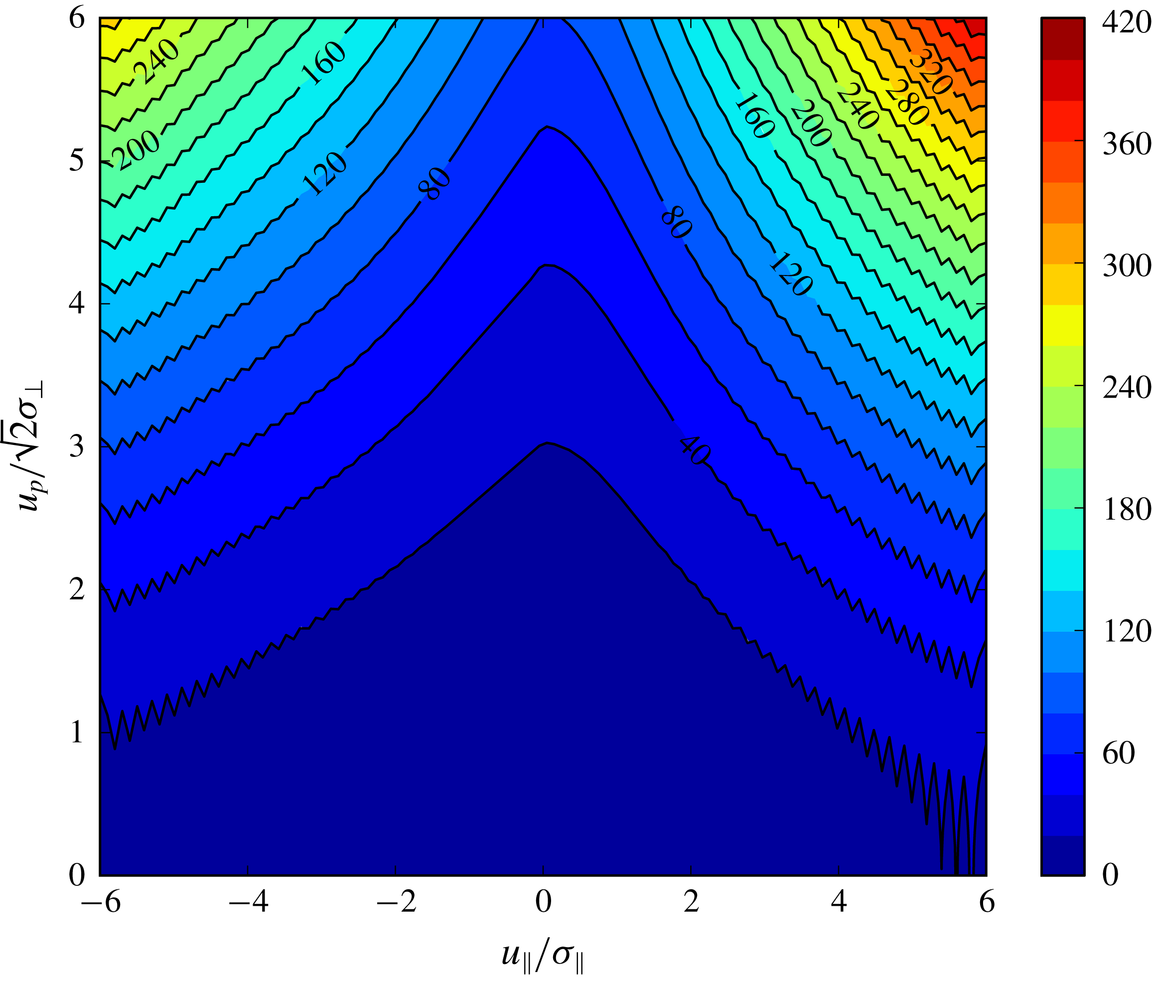
Figure 12 shows the mean-square separation for the four different values of
 $r_{0}$
. It is disappointing that the curves do not collapse into a single curve but the limited inertial subrange of the DNS is the most likely explanation for this behaviour; indeed, Sawford & Yeung (Reference Sawford and Yeung2010) present a similar plot to figure 12(b) (for their Q1D model rather than their Q2D model) in which the curves also do not collapse. The curve with
 $r_{0}/\unicode[STIX]{x1D702}=4$
appears to be beginning to follow a
 $t^{3}$
scaling giving
 $g_{f}\approx 0.8$
; the curve with
 $r_{0}/\unicode[STIX]{x1D702}=2$
also shows scaling close to
 $t^{3}$
but with
 $g_{f}\approx 0.38$
. For comparison, Sawford & Yeung (Reference Sawford and Yeung2010) obtain a value of
 $g_{f}=0.4$
with their Q2D model for the same value of
 $R_{\unicode[STIX]{x1D706}}$
. At small
 $t$
there is a period when the growth of
 $\langle r^{2}-r_{0}^{2}\rangle$
is slower than quadratic in
 $t$
. This could be a sign of an incipient regime proportional to
 $t$
as in figure 7.
The results for the equivalent backwards dispersion model are presented in figure 13. Compared with figure 12,
 $\langle r^{2}\rangle$
increases more rapidly in the nascent
 $t^{3}$
regime (where the growth is actually more rapid than
 $t^{3}$
); similar differences were observed for DNS by Buaria et al. (Reference Buaria, Sawford and Yeung2015, see figure 2) and Sawford et al. (Reference Sawford, Yeung and Borgas2005, see figure 4). As in figure 12, the curves with
 $r_{0}/\unicode[STIX]{x1D702}=4$
and
 $r_{0}/\unicode[STIX]{x1D702}=2$
show some indication of a nascent inertial subrange with
 $t^{3}$
scaling (though again disappointingly not at the same value of
 $r^{2}/\unicode[STIX]{x1D700}t^{3}$
as each other). The values of
 $g_{b}$
for these two curves are respectively 2.85 and 1; For reference, Sawford & Yeung (Reference Sawford and Yeung2010) obtain a value of
 $g_{b}=2$
with their Q2D model for the same value of
 $R_{\unicode[STIX]{x1D706}}$
. Compared with the forwards model (see figure 12
b), there is less indication of a period of slower than quadratic growth at small
 $t$
in the backwards case.
The ratio
 $g_{b}/g_{f}$
is shown in figure 14 and shows that, for
 $r_{0}/\unicode[STIX]{x1D702}=4$
and
 $r_{0}/\unicode[STIX]{x1D702}=2$
, it is approximately 3. This is consistent with the analytical model presented above and with previous results (Berg et al.
Reference Berg, Lüthi, Mann and Ott2006; Sawford & Yeung Reference Sawford and Yeung2010; Buaria et al.
Reference Buaria, Sawford and Yeung2015; Bragg et al.
Reference Bragg, Ireland and Collins2016). The variation of this ratio with
 $r_{0}$
is similar to that found by Bragg et al. (Reference Bragg, Ireland and Collins2016, see figure 1).
The mean-square separation (a) and its compensated form (b) using the form of
 $p_{u_{\Vert }}(u_{\Vert })$
extracted from the DNS data of Sawford & Yeung (Reference Sawford and Yeung2010):
 $r_{0}/\unicode[STIX]{x1D702}=2$
(solid);
 $r_{0}/\unicode[STIX]{x1D702}=4$
(dashed);
 $r_{0}/\unicode[STIX]{x1D702}=8$
(dotted);
 $r_{0}/\unicode[STIX]{x1D702}=16$
(dot-dashed). The Kolmogorov time scale is indicated by
 $\unicode[STIX]{x1D70F}_{\unicode[STIX]{x1D702}}$
.

As figure 12 but for the backwards dispersion model using the DNS-based form of
 $p_{u_{\Vert }}(u_{\Vert })$
.

The ratio of the DNS backwards (indicated by subscript
 $b$
) to forwards (
 $f$
) mean-square separation. The initial separations are the same as those in figure 12.

7 Conclusions
A non-Gaussian two-particle LSM has been developed that includes the effect of non-zero skewness in the longitudinal relative velocity distribution. This has been achieved by requiring the Eulerian p.d.f. of the longitudinal relative velocity component to be consistent with the four-fifths law of turbulence. As may be expected, the effect of a negative skewness in the Eulerian relative velocity p.d.f. is to reduce the mean rate of separation of the pairs and to reduce the skewness of the separation. Compared with the equivalent Gaussian model, the value of Richardson’s constant is closer to that observed experimentally and in DNS. The value in the corresponding non-Gaussian backwards dispersion model is approximately a factor of 2.9 larger than the forwards model which is consistent with results obtained from DNS and experimentally.
The model was formulated in spherical polar coordinates. We showed that in isotropic turbulence, any 3-D model for the relative separation reduces to a Q2D model regardless of the choice of the velocity distribution
 $p_{E}$
or the particular modelling choices. In designing the model, we assumed for simplicity that
 $p_{E}$
can be separated into the product of the p.d.f.s of the longitudinal and transverse velocities. Although this separation is not well justified, it is difficult to do more than speculate about the precise effects of this assumption. That the ratio
 $g_{b}/g_{f}$
is consistent with previous results is encouraging and suggests the model is behaving correctly. To test this would require the development of a model which satisfies the incompressibility constraints on
 $p_{E}$
. We also restricted attention to models in which the transverse conditional mean accelerations are quadratic in velocity. The resulting model is still non-unique but can be determined by choosing the longitudinal and transverse velocity probability distributions and making a choice for the model parameter
 $\unicode[STIX]{x1D719}(r)$
(described in § 2.2). For a particular choice of
 $\unicode[STIX]{x1D719}(r)$
we showed that the model reduces to the Q1D model of Kurbanmuradov (Reference Kurbanmuradov1997) provided only that the shape of the transverse velocity p.d.f.
 $p_{u_{p}}$
is independent of separation. To fix our model we used Gaussian transverse velocity distributions, a particular choice of longitudinal velocity distribution satisfying the four-fifths law, and chose
 $\unicode[STIX]{x1D719}(r)$
to match the model of Thomson (Reference Thomson1990).
The variation with
 $C_{0}$
of our non-Gaussian model and the corresponding Gaussian model was considered. We showed that, as expected, for large
 $C_{0}$
the Gaussian and non-Gaussian models tend to the analytical result from the associated diffusion equation (although the rate of convergence is slower for the non-Gaussian model than for the Gaussian model). Analytic results for
 $C_{0}=0$
were also obtained and, although this value of
 $C_{0}$
is not physically appropriate, the results for
 $C_{0}=0$
, together with the diffusive large
 $C_{0}$
results, help to explain the behaviour for intermediate values of
 $C_{0}$
.
An equivalent model using a numerical form of the longitudinal relative velocity p.d.f. obtained from DNS data was presented in § 6. The lack of a substantial inertial subrange in the DNS data militates against a reliable estimate of Richardson’s constant. Nonetheless the values of
 $g_{f}$
and
 $g_{b}$
that were found in § 6, though different from both the analytical model and the results of Sawford & Yeung (Reference Sawford and Yeung2010), were still of the same order of magnitude. In particular, the ratio
 $g_{b}/g_{f}$
was similar to that obtained with the analytical model and previous results. The differences with the analytical model are likely to be due to the nature of the DNS data, principally the limited inertial subrange and the shape of
 $p_{u_{\Vert }}$
, while the differences with the Q2D model of Sawford & Yeung (Reference Sawford and Yeung2010) are most likely due to the relationship that we assume between the conditional mean acceleration and
 $p_{u_{\Vert }}$
(as discussed in § 6).
Acknowledgement
The authors would like to thank B. Sawford for providing the DNS data used in § 6.



