

How do elections affect the economy? Most work on this question examines whether elections alter the economic policies of incumbent governments. In particular, theories of ‘opportunistic’ political business cycles suggest that policymakers induce short-term economic expansions immediately before elections with the expectation that the gains will subside soon after the votes have been cast.Footnote 1 A separate line of work argues that left-wing governments pursue low unemployment at the expense of higher inflation while right-wing governments prioritize low inflation at the expense of higher unemployment. The rational partisan theory, for instance, holds that partisan priorities and uncertainty about the electoral outcome cause a post-election increase (decrease) in unemployment if the left- (right-) wing party wins.Footnote 2
We argue that a major and underappreciated impact of elections is that they generate policy uncertainty that encourages individuals and businesses to delay certain types of investments until the race concludes. These investments are ones that would be impossible or costly to reverse; scholars have termed them ‘irreversible investments’.Footnote 3 Examples include housing or automobiles for individuals and fixed capital for businesses. In the sectors associated with such investments, the incentive for delay causes a pre-election decline. Moreover, because the incentive derives from the policy uncertainty associated with the election, the decline is larger if there are greater policy differences between the major parties/candidates and if the race is more competitive.
We test the arguments about irreversible investment, elections and uncertainty using survey and behavioural data that involve a canonical irreversible investment: housing. We collected the survey data in conjunction with the 2008 Cooperative Congressional Election Survey (CCES), which involved pre- and post-election waves in association with the 2008 US elections.Footnote 4 The survey analysis compares a respondent's pre-election perceptions of how much the presidential election outcome will affect his or her financial situation with post-election accounts of whether he or she delayed housing-related activities and purchases until learning the outcome. Notably, only some of these activities are irreversible investments, and therefore the theoretical arguments do not always predict a significant relationship. The survey analysis can therefore repudiate the theory by finding an effect when one is not predicted, and can fail to find an effect when one is predicted.
The second type of test involves data on US housing markets. Specifically, we make use of the staggering of US gubernatorial elections across time and states to analyse whether the variation in gubernatorial electoral cycles is associated with variations in state and local housing markets. Because the theoretical arguments apply most directly to the quantity of sales, we begin by analysing this factor using Zillow.com data from thirty-five states from 1999–2006. We then discuss conditions under which the arguments apply to home prices and examine price data from over 300 metropolitan statistical areas from 1979–2006.
The article begins by reviewing the research on irreversible investment. The second section develops the theoretical argument and compares it to other perspectives. The third section describes the survey analysis, and the fourth section examines the housing markets. We conclude by discussing the implications of the analysis for understanding the impact of elections on the economy.
Research on irreversible investment
Various formal models analyse the incentive to delay irreversible investments when economic uncertainty is high.Footnote 5 The original models focused on business decisions, and show that delay can be optimal – even for a risk-neutral firm that incurs costs from postponing the investment. The firm's incentives depend on how soon the new information will be revealed, the value of the information, the costs of delay and the costs of undoing the investment (if doing so is even possible). Subsequent scholarship applied these theories to consumer behaviour and established that economic uncertainty can induce individuals to postpone costly-to-undo investments such as homes and consumer durables.Footnote 6 Housing is a prominent irreversible investment, given the high transaction costs associated with undoing the purchase and because households devote significant savings to it;Footnote 7 as Christopher Carroll and Wendy Dunn note, housing is the ‘mother of all durable goods’.Footnote 8
Some studies have conjectured that political events are an important source of economic uncertainty, but this possibility has more typically been ‘discussed casually’ rather than scrutinized, to quote George Bittlingmayer.Footnote 9 Bittlingmayer offers evidence within the context of a major historical shift; in particular, he demonstrates that the switch from Imperial to Weimar Germany induced stock market volatility and output declines.Footnote 10 Likewise, Nicholas Bloom shows that major wars and acts of terrorism can induce stock market volatility.Footnote 11 However, even Bittlingmayer and Bloom do not offer evidence that the associated political uncertainty of more routine political events, let alone elections, affects irreversible investment.
Theoretical framework
Because others have already developed formal theories of irreversible investment and applied them to the housing industry, in the interest of space we will not construct a full formalization. Instead, we begin by justifying the argument that elections are a key source of uncertainty and then delineate how this uncertainty affects individuals’ and firms’ incentives. We proceed to argue that this impact depends on the policy differences between the major parties/candidates and electoral competitiveness.
Elections and Uncertainty
Elections are an important source of economic uncertainty, due to the fact that the outcome of a race affects subsequent government decisions. As Andrea Mattozzi summarizes, ‘Political uncertainty…arises because different candidates running for office, if elected, will implement different policies’.Footnote 12 These differences encompass fiscal as well as regulatory policies. Moreover, the policies may target a specific industry or be designed to affect society more broadly.
Regarding fiscal policy, a range of work suggests that conservative parties prefer lower spending on domestic programs and lower taxes than progressive parties do; this generalization has received support in a variety of countries, including the United States, where the difference holds at the national and state levels.Footnote 13 In other words, for individuals and firms, the outcome of an election may affect their income and/or tax rates. For an individual, such an effect might occur if his or her taxes were likely to change under a new government; if his or her job were associated with government employment, government contracting or an industry closely associated with public programs; or if his income depended on government benefits that the left- or right-wing party would likely alter. As these examples suggest, the uncertainty will not be identical across society but instead vary according to the likely effects of the candidates’/parties’ policies.
Indeed, some types of fiscal policies are even targeted to particular investments or industries. For instance, the Obama administration has proposed reducing the mortgage-interest tax deduction for high-income households. This policy, if enacted, would effectively increase the cost of home mortgages for these households.Footnote 14 At the US state level, some governments have limited the ability of localities to raise property taxes and have provided property tax relief to certain classes of homeowners.Footnote 15
Parties differ over not only fiscal policies but also regulatory policies that favour different mixes of industries. For example, environmental regulations that support alternative energy sources may increase the profitability of these businesses as well as the desirability of cars or homes that use such energy sources.Footnote 16 With respect to housing, industry- or firm-specific regulations can also influence the value of homes that are located near a firm that is affected by the regulations. Moreover, research suggests that homeowners are aware of these effects. For instance, Kenneth Scheve and Matthew Slaughter find that individuals care about the effects of trade policies on local firms due to their ensuing effects on local home prices.Footnote 17
Finally, elections create economic uncertainty for some individuals due to their impact on the individuals’ employers. Research on the timing of contract negotiations suggests that firms tend to delay negotiations until after elections because of the policy uncertainty they create.Footnote 18 Accordingly, workers who are aware that their contract will be reviewed after an election may associate it with economic uncertainty even if they are not personally following the race closely. In sum, the policy uncertainty associated with elections engenders economic uncertainty for individuals and firms through a variety of mechanisms.
Incentives for Irreversible Investment
Because elections induce uncertainty, individuals and firms can have the incentive to delay costly-to-undo investments until after electoral outcomes are realized. Consider a given individual or firm X that is interested in making an investment i, and assume the election outcome affects the optimal type or level of investment. The investment is irreversible; for simplicity, assume it cannot be undone. (Alternatively, one could assume it can only be undone at a high cost, and incorporate how these costs affect X's incentives.) If X delays the investment until after the election, X chooses the optimal investment i*. Delaying the investment postpones the utility and/or profits that X receives from the investment, however, and therefore carries a cost c. If X commits to an investment before the election, then X avoids the cost c but risks choosing an investment that is not first best, given the information that is subsequently revealed. The question for X is thus whether the expected utility from i* (versus that of the pre-election investment) outweighs the cost of delay c.Footnote 19
In the previous subsection, we substantiated the claim that elections create policy uncertainty. Therefore it seems reasonable to expect that the benefits of waiting will commonly outweigh the costs associated with doing so. If this expectation is correct, then on average elections will be associated with a pre-election decline in irreversible investment. That is, if we examine all elections together as a group, we should expect to observe a pre-election decline. We will refer to this hypothesis as the Pre-election Decline Prediction.
Policy Differences and Irreversible Investment
The discussion thus far has emphasized that the incentive for delaying costly-to-undo investments derives from the policy differences between the major parties/candidates. Yet elections are not identical in terms of the policy differences between the parties. In some cases, the parties’ positions might be relatively similar, while in other cases they might propose drastically different approaches to economic issues. Likewise, even within a given election, the policy differences between the parties will not affect all individuals similarly. For instance, one party could propose to freeze the pay of federal workers, which would clearly affect public employees more than private ones. Similarly, the Obama administration's proposal to reduce the mortgage deduction for higher-income individuals would affect these individuals more than others.
This variation across elections and individuals suggests that the effect of elections on irreversible investment will depend on the policy differences between the major competitors. In particular, as the polarization between the major parties/candidates increases, the incentive to delay irreversible investments until after the election will also increase. We label this the Policy Differences Prediction. It suggests that the larger the effects of an electoral outcome on an individual's financial situation, the more likely she should be to delay costly-to-undo investments. Likewise, the hypothesis implies that as the policy differences between parties/candidates expand, sectors associated with irreversible investment should experience a larger downturn.
Electoral Competitiveness and Irreversible Investment
Elections vary not only in terms of the policy differences between the major parties/candidates, but also with respect to the competitiveness of the race. In some elections, a party/candidate holds a convincing lead throughout the campaign, while in other cases the race is highly competitive. As competitiveness increases, individuals and firms will be less able to predict the types of policies that the government will support after the election; consequently, the benefits of delaying costly-to-reverse investments grow. We therefore expect that the more competitive a race is, the larger the decline in irreversible investment will be. We call this the Electoral Competitiveness Prediction.
Notably, if the outcome is highly predictable, then the election may engender so little policy uncertainty that the benefits of postponing irreversible investments may be trivial. In that case, individuals and firms would have little incentive to bear the costs associated with delay. The Electoral Competitiveness Prediction does not specify a threshold beyond which an election is insufficiently competitive to generate a pre-election decline in irreversible investment, but it allows for this possibility. In the empirical analysis of housing markets, we will assess whether such a threshold exists.
Comparison with other Theoretical Perspectives
These theoretical predictions and framework, which we will refer to as the Electoral Investment Theory, contrast with other perspectives of how elections influence the economy. It is worth highlighting the differences with three major alternatives: opportunistic political business cycle theories, partisan business cycle theories and recent work on how mass partisanship influences consumer behaviour. Consider the opportunistic perspective, in which incumbents engineer a pre-election expansion through fiscal and/or monetary policies.Footnote 20 Some scholarship suggests that this cycle will not occur if an incumbent is highly popular (and therefore quite likely to win re-election)Footnote 21 or quite unpopular.Footnote 22 Other work indicates that opportunistic cycles are larger in countries with higher levels of polarization.Footnote 23 Thus in contrast to the Electoral Investment Theory's predictions, the opportunistic perspective suggests that the pre-election period is associated with an expansion that increases with electoral competitiveness and elite-level polarization.
The next set of alternatives is called ‘partisan’ theories because they assume that growth and employment are lower under right-wing governments. According to Douglas Hibbs, in the traditional partisan cycle this lower growth does not depend on the electoral cycle.Footnote 24 Conceptions of growth do vary in the rational partisan theory of Alberto Alesina, John Londregan and Howard Rosenthal, but still there is no pre-election contraction. As they assert, in the latter half of a term, ‘the economy returns to its “normal” rate of growth, implying that there is not a “partisan” influence on the rate of growth in the second half of each term’.Footnote 25 Notably, the growth rate is normal regardless of the level of electoral competitiveness or polarization between the parties.Footnote 26
Recent work by Alan Gerber and Greg Huber about the impact of mass partisanship on consumer behaviour is perhaps closest to the predictions of the Electoral Investment Theory.Footnote 27 Gerber and Huber find that in the months following a US presidential election, a county's sales tax receipts positively correlate with its level of support for the electoral winner. This effect differs from the Electoral Investment perspective in important respects, however. First, Gerber and Huber do not predict a pre-election decline. Secondly, they do not distinguish between irreversible investment and other types of purchases. Thirdly, in Gerber and Huber the aggregate change between the pre- and post-election periods decreases with electoral competitiveness. By comparison, the Electoral Competitiveness Prediction suggests that the change should increase as the race becomes tighter.
In sum, existing theoretical perspectives do not predict any sort of pre-election decline in irreversible investment, let alone relate such a decline to electoral competitiveness or polarization between the major parties. The following analyses assess these new predictions using survey and housing market data.
Survey analysis
We conducted the survey as part of the 2008 CCES, which encompassed a set of nationally representative modules purchased by individual universities/groups. Each module included questions written by that group as well as a core content of profile items about the respondent's background and questions designed to be of interest to a range of social scientists. The 2008 CCES consisted of a pre- and post-election wave, with 1,000 respondents per module in the initial wave.
In the first wave we asked about the extent to which the electoral outcome would affect various aspects of the respondent's financial situation, including his or her job security, taxes and income. The question was worded, ‘Now I'd like you to consider some different factors that may affect your personal financial situation. For each of these factors, how much difference do you think it will make who wins the upcoming presidential election…A big difference, some difference, only a little difference, or no difference at all?’ This four-point scale is commonly employed in questions about financial matters.Footnote 28 The specific factors included ‘job security’, ‘the amount of taxes you pay’ and ‘personal income’. In the post-election wave we asked whether the respondent had delayed certain purchases and actions until after the election. The precise question was, ‘Please tell me whether you put off any of the following things until you knew the results of the November elections…’ The possible answers were ‘yes’ or ‘no’.
We solicited this information for three related items, only two of which are canonical irreversible investments. The irreversible investment-related items were ‘buying or selling a home’ and ‘undertaking a home renovation’. We also included a quasi-placebo item (‘moving’) to ensure that any effects uncovered for home transactions or renovations were not due to certain respondents having a tendency to delay all actions until after the election. We chose moving because the activity is correlated with housing investments yet, given the option of renting, still distinct. Research suggests that moving itself is heavily influenced by family events such as marriage, divorce and childbearing.Footnote 29
The Policy Differences Prediction suggests that the likelihood that individuals will delay irreversible investments should be affected by perceived policy differences between the candidates. At the same time, these policy differences should not be associated with the likelihood of moving. To assess whether these relationships hold, we conducted a separate probit regression for each combination of pre- and post-election items. The dependent variables, Delay Moving, Delay Renovation and Delay Home Purchase/Sale, each equal 1 if the respondent stated that she had delayed the activity until after learning the election results, and 0 otherwise. The key independent variables were rated using a four-point scale that corresponds to how much difference the election would make. Specifically, Job Security Difference equals 0 if the respondent stated that it made no difference who won the election for her job security, 1 if ‘only a little difference’, 2 if ‘some difference’ and 3 if ‘a big difference’. Tax Difference and Income Difference were coded similarly. The combination of the pre- and post-election items creates nine separate regressions.
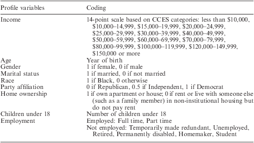
These regressions include demographic and political controls to account for the possibility that particular groups were disposed to delay actions until after the election. The control variables, which are from the CCES core content, account for age, gender, marital status, race, political party affiliation, income, homeownership and number of children under eighteen. The coding is based on the CCES categories and described in Table 1. We also controlled for respondents’ confidence about future income using the CCES common content question ‘How would you guess your total family income to be six months from now?’ The available responses were ‘higher’, ‘the same’ or ‘lower’, which we coded as an ordinal three-point scale. Including this variable helps ensure that any observed effects of the policy difference variables are not a function of respondents’ general anxiety about future income; without this control, the results still support the Policy Differences Prediction, as shown in the web appendix. Finally, as discussed below, we also split the sample by certain control variables in an effort to ascertain whether the findings are driven by particular types of respondents.
CCES Profile Variables in Survey Analysis

We analysed all available survey observations in each regression. Almost 200 of the pre-election CCES respondents did not participate in the post-election wave, and respondents often failed to provide basic profile information in the pre-election wave. Given these constraints, we received a high proportion of responses. For each combination of pre- and post- items, the response rate was a minimum of 97 per cent of those who provided the basic profile information (Table 1). The number of potential respondents was 697 for the Tax Difference question (which was asked of everyone) and 385 for the Job Security Difference and Income Difference questions (which were asked of all those that reported working full or part time according to the profile item on employment).
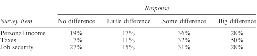
As is standard, the CCES survey weights are used in the data analysis in order to minimize any sample-related bias. For instance, if the proportion of retirees that participated is lower than expected, then the retirees who did participate receive a higher weight. The CCES target population is the national US adult population, and the CCES used the 2006 American Community Survey to design the weights. Further details on the weighting are given in the 2008 CCES guide.Footnote 30Table 2 describes the distribution of the weighted responses for the policy difference questions.Footnote 31
Survey Responses, Perceived Policy Differences
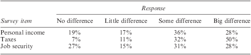
Note: The data describe the distribution of weighted responses for the survey items analysed in Table 3.
Notably, each item produced a different distribution of responses. Only 7 per cent of respondents believed that the election would make no difference with respect to their taxes, 11 per cent that it would make little difference, 32 per cent some difference and 50 per cent a big difference. By contrast, 27 per cent of respondents believed the election would have no effect on their job security, close to the same percentage that believed the election would have some effect (31 per cent) or a big effect (28 per cent). For personal income, 19 per cent believed the election would have no effect, 17 per cent little effect, 36 per cent some effect and 28 per cent a big effect.
The post-election responses about the likelihood of delay were more stable: 14 per cent of individuals reported that they delayed purchasing or selling a home, 16 per cent postponed home renovations and 13 per cent postponed a move. Despite this stability, however, the correlation between the items was not particularly high. For instance, the correlation between postponing renovations and moving was ρ = 0.5 and between a home sale/purchase and renovations only ρ = 0.6. Of the ninety-four respondents who professed that they had delayed buying or selling a home until after the election, more than one-quarter did not delay moving.
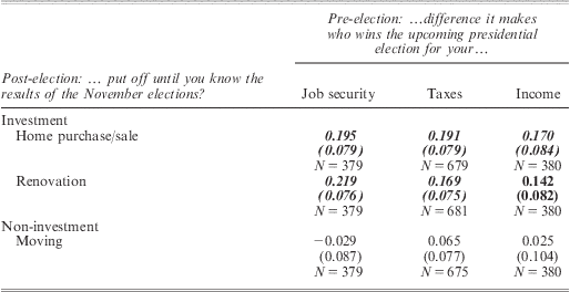
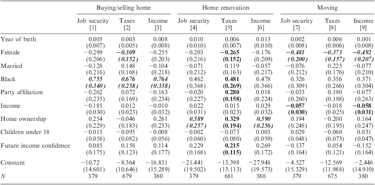
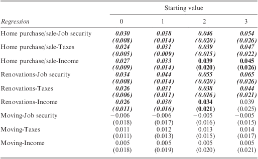
The critical question is whether this variation relates to the variation across respondents in how much they perceived that the election would affect their personal finances. Table 3 presents the key results for each probit regression. Parameter estimates for the control variables are provided in Table 4.
Test of the Policy Differences Prediction, Survey Analysis
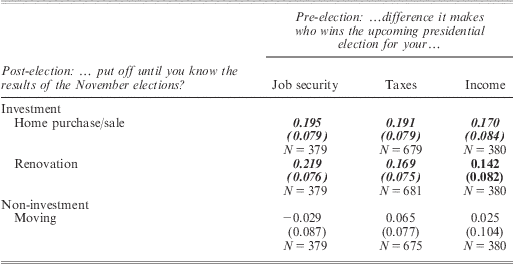
Note: Probit coefficients given above standard errors. Controls include age, gender, race, marital status, party affiliation, income, number of children under eighteen, home ownership and future income confidence. Results for the control variables are detailed in Table 4. Parameter estimates in bold are significant at p < 0.1 (two-tailed), and estimates in bold italics are significant at p < 0.05 (two-tailed).
Control Variable Results for Survey Analysis
Note: Probit coefficients given above standard errors. Estimates in bold are significant at p < 0.1 (two-tailed), and estimates in bold italics are significant at p < 0.05 (two-tailed). Table 3 presents the results for the variables that test the Policy Differences Prediction.
The analysis strongly supports the Policy Differences Prediction. As the rows in Table 3 regarding home transactions and renovations show, the greater the effect of the election on a respondent's financial circumstances, the more likely she is to postpone these irreversible investments until after the election. Moreover, in every case but one this effect is significant at p < 0.05, two-tailed, and even the exception is significant at p < 0.1, two-tailed. By contrast, the effect of the quasi-placebo item (moving) is never significant by any conventional standard.
The magnitudes of the estimates further suggest that the incentive to delay costly-to-undo investments relates to candidates’ policy differences. Table 5 presents the marginal effects for every combination of pre- and post-election item. These effects are calculated at each level of policy difference on the four-point scale – no difference (0), only a little difference (1), some difference (2) and a big difference (3) – holding all control variables at their means. For each of the irreversible investments, the marginal effect is larger for higher values of the policy difference scale.
Marginal Effects, Survey Analysis of Policy Differences Prediction
Note: Marginal effects given above standard errors. Estimates in bold are significant at p < 0.1 (two-tailed), and estimates in bold italics are significant at p < 0.05 (two-tailed).
The first row of results concerns home transactions and how much the electoral outcome affects job security. A shift from perceiving that the election makes no difference to a little difference increases the likelihood of delay by 3 percentage points, while a shift from some difference to a big difference increases the likelihood by 5.5 percentage points. For renovations, the analogous changes increase the probability of delay by 3.5 and 6.5 percentage points, respectively. These marginal effects are even more substantial when one considers larger changes. For instance, a shift from perceiving a big effect on taxes to perceiving no effect reduces the likelihood of delaying a home sale/purchase by 14 percentage points (0.047 × 3). By comparison, the marginal effects on the quasi-placebo item of moving are substantially smaller in magnitude (as well as statistically insignificant).
The estimates for the control variables, reported in Table 4, suggest that perceived policy differences were not the only factors that influenced respondents’ decisions. Blacks were more likely than others to delay home purchases/sales, women were less likely than men to postpone moves and homeowners were more likely than others to delay renovations. Also, there was some evidence that women were less likely than men to postpone home purchases and higher-income individuals were less likely to delay moves.
We separately investigated whether the results were driven by certain subgroups of the population, including party members and homeowners. Partisans may be more emotionally invested in the election, and therefore more likely to delay actions and/or believe it will have greater policy implications. Party members are defined as those who identify as Democrats or Republicans in the coding for the control variable regarding party affiliation. If we add to the regressions an interaction term between party membership and the perceived policy difference plus a main effect for party membership, the coefficient on the interaction term is never significant (p > 0.3, two-tailed). If we instead run separate regressions for party members and unaffiliated respondents, party membership appears to matter in the expected direction for the renovations-job regressions, but in the opposite direction for the renovations-tax analysis.Footnote 32 Even more basic t-tests find that the responses do not differ significantly according to party membership. Overall, the evidence suggests that support for the Policy Differences Prediction does not derive solely from partisans.
One could envision that the results might vary according to home ownership. Homeowners could be more affected if they are concerned about the possibility of holding two mortgages, or alternatively less affected if they are buying and selling simultaneously. In nested tests, there is no evidence of a difference between homeowners and others; with the addition of an interaction term between home ownership and the policy difference variable, the hypothesized effects are never significantly larger for homeowners, with or without interactions between home ownership and the controls. However, if instead the sample is split and separate (non-nested) regressions are run, the hypothesized effect of perceived policy differences on irreversible investment is always significant with the homeowner sample (p < 0.05, two-tailed) and never significant at conventional levels with the non-homeowner sample. These results change somewhat if we consider non-homeowners with incomes of at least $40,000. The hypothesized effects then hold at conventional significance levels (p < 0.05, two-tailed) in analyses of tax policy differences. The supplemental tests thus suggest that homeowners may be more affected than others, although the null results from the nested tests indicate that one cannot make strong conclusions about the issue from these data.
In sum, the survey analysis provides strong support for the Policy Differences Prediction. The larger the impact that the individual perceived the election would have on her personal financial situation, the more likely she was to delay irreversible investments until after the election. No such effect occurred for the quasi-placebo item. The results are thus highly supportive of the theory.
At the same time, one could argue that the 2008 campaign was special in many ways: the housing market was in turmoil, this turmoil led to a collapse of financial markets and the presidential election involved the unexpected rise of Barack Obama. None of these events, of course, implies that the propensity to delay irreversible investments would necessarily be correlated with respondents’ perceptions of policy differences between the candidates. Moreover, the analysis of the quasi-placebo item suggests that the events did not cause respondents who perceived larger policy differences to delay all decisions. Still, we recognize that any given election may have qualities that make it uncharacteristic. For this reason, we proceed to examine data that involve housing markets across scores of elections.
Housing market analysis
The examination of housing market data is advantageous for several reasons. Perhaps most obviously, it offers a straightforward assessment of market activity: if people are indeed delaying purchases until after an election, then the sales records should reveal this pattern. Furthermore, there is substantial regional variation in the US housing market,Footnote 33 and a variety of US state government policies affect individuals’ incentives with respect to housing purchases. Accordingly, we can assemble a dataset with cross-sectional as well as over-time variation.
Like the national government, US state governments may influence an individual's taxes and job security. For example, state-level income taxes are as high as 11 per cent and state governments directly employ almost four million individuals. Moreover, these governments enact many laws that explicitly deal with real estate. As mentioned previously, states can limit the ability of localities to raise property taxes and can directly provide property tax relief to groups of homeowners.Footnote 34 State governments also influence housing markets through policies that attract businesses to particular locations. For instance, when a state creates or expands tax-free zones for businesses, then the tax-free areas become more desirable.Footnote 35 Likewise, state governments can offer tax credits to firms to encourage them to move to the state, and such relocations affect local housing markets.Footnote 36 More generally, as Michael Ebeid and Jonathan Rodden note, US state governments have ‘wide-ranging control over fiscal and regulatory policy’.Footnote 37
Thus if the Electoral Investment Theory is correct, gubernatorial elections should affect state and local housing markets. An advantage of focusing on gubernatorial elections is that we can exploit the sub-national variation in these electoral cycles.Footnote 38 Gubernatorial elections are staggered such that in every year multiple states have an election. The analysis can therefore use year indicators to control for national influences and assess whether states with gubernatorial elections in a given year have weaker housing markets than other states. Of course, the tests will also account for local variations in the economy, demographics and other factors.
We examine two measures of housing market performance. First, Zillow.com offers data on home sales, as a percentage of all homes, for thirty-five states from 1999–2006. These data allow us to analyse seventy-three gubernatorial elections.Footnote 39 Secondly, as a supplementary analysis, we use the Conventional Mortgage Home Price Index (CMHPI), which is published by the Federal Home Loan Mortgage Corporation (Freddie Mac) and encompasses over 300 metropolitan statistical areas (MSAs).Footnote 40 For some MSAs, the index extends back as far as 1975. Due to the more limited time span of some of the control variables, the CMHPI is examined from 1979–2006 for 338 MSAs. These data encompass 339 separate gubernatorial elections.
The measure of sales clearly offers a more direct test of the theoretical predictions. However, research on housing markets suggests that new home construction is strongly persistent and that correspondingly, supply responds more slowly than demand to external dynamics.Footnote 41 If one takes these stylized facts as given, then demand should respond more than supply to the political uncertainty engendered by an upcoming election. We therefore analyse price data in addition to the sales data, but focus on the analysis of sales, given that it does not depend on additional stylized facts and assumptions.
For the data on sales, we test the Pre-election Decline and Electoral Competitiveness Predictions using the following general specifications for each state i and year t:
 $${\rm{\% Homes}}\,{\rm{Sol}}{{{\rm{d}}}_{{\rm{it}}}} = f({\rm{Gubernatorial}}\,{\rm{Election}}\,{\rm{Yea}}{{{\rm{r}}}_{{\rm{it}}}}{\rm{,}}\,{\rm{Sub - National}}\,{\rm{Control}}{{{\rm{s}}}_{{\rm{it}}}}{\rm{,}}\,{\rm{Year}}\,{\rm{Indicator}}{{{\rm{s}}}_{\rm{t}}}{\rm{,}}\,{{{\rm{\eta }}}_{\rm{i}}}{\rm{)}}
$$
and
 $$\displaylines{
{\rm{\% Homes}}\,{\rm{Sol}}{{{\rm{d}}}_{{\rm{it}}}} = & f({\rm{Gubernatorial}}\,{\rm{Election}}\,{\rm{Yea}}{{{\rm{r}}}_{{\rm{it}}}}\times {\rm{Competitiv}}{{{\rm{e}}}_{{\rm{it}}}}{\rm{,}}\,{\rm{Gubernatorial}}\, \cr
& {\rm{Election}}\,{\rm{Yea}}{{{\rm{r}}}_{{\rm{it}}}}\times {\rm{Not}}\,{\rm{Competitiv}}{{{\rm{e}}}_{{\rm{it}}}}{\rm{, Competitiv}}{{{\rm{e}}}_{{\rm{it}}}}{\rm{,}}\, \cr
& {\rm{Sub - National}}\,{\rm{Control}}{{{\rm{s}}}_{{\rm{it}}}}{\rm{,}}\,{\rm{Year}}\,{\rm{Indicator}}{{{\rm{s}}}_{\rm{t}}}{\rm{,}}\,{{{\rm{\eta }}}_{\rm{i}}}{\rm{),}} \cr}$$
where ηi represents state fixed effects. The general specifications for home prices are analogous for each MSA m and year t except that some controls are available at the MSA level while others are only available at the state level. The following descriptions clarify the level at which each control is available. Summary statistics are given in the web appendix.
%Homes Sold
Zillow.com calculates the percentage of single-family homes that sold within a given state and year out of all single-family homes in that state, whether they were explicitly on the market or not. %Homes Sold equals this value, which captures turnover in the single-family housing market. Importantly, the measure is based on both new construction and ‘existing’ homes. Obtaining an accurate estimate of total home sales is important for interstate comparisons because new homes are a more significant portion of some markets than others. Also beneficial is the fact that the Zillow.com data are based on actual sales, not pending contracts that may ultimately fall through. By comparison, the US government collects data on sales of new homes versus existing homes separately, and the series are not compatible. The series on new homes is not even available at the state or local levels. Moreover, it is based on pending contracts, while the existing home sales series reflects actual purchases.Footnote 42
%Change in Real Home Prices
The CMHPI is constructed from over thirty million ‘repeat transactions’. A particular home's value must be observed at least twice in order for that home to contribute to the price index. This feature, and the breadth of the data, makes the CMHPI attractive to scholars.Footnote 43 The index encompasses not only high-profile metropolitan statistical areas such as the one that incorporates both Boston and Quincy, Massachusetts but also lower profile areas such as Altoona, Pennsylvania.Footnote 44 The index is based on conventional, conforming mortgages for single-unit residency houses purchased or securitized by the Federal Home Loan Mortgage Corporation (Freddie Mac) or the Federal National Mortgage Association (Fannie Mae). All data are converted to 2008 dollars for the purposes of analysing real prices; the results are robust to analysing nominal prices. Due to the substantial variation in price across localities, we follow the standard practice of analysing percentage change rather than the absolute level, although the substantive results are robust to using the absolute level.Footnote 45
Gubernatorial Election Year
This key independent variable equals 1 if the state has a gubernatorial election that year and 0 otherwise.
Electoral Competitiveness
We measure electoral competitiveness as a function of the winning gubernatorial candidate's share of the two-party vote.Footnote 46 For the data on home sales, the median value of this share is 55 per cent and for prices it is 56 per cent. To minimize collinearity among interaction terms, we categorize races as either competitive or uncompetitive. Specifically, Competitive equals 1 if the winner receives less than 55 per cent of the two-party vote and 0 otherwise. Likewise, Not Competitive equals 1 if the winner receives at least 55 per cent of the vote and 0 otherwise. We have experimented with alternative cut points, and the results are robust to alternatives.Footnote 47
Real Income Growth
Various studies suggest that home prices increase in response to growth in personal income.Footnote 48 To account for this influence, we use US Bureau of Economic Analysis personal income data. These data are available at the state and MSA levels, and each test uses the level consistent with that of the dependent variable (state level for home sales and MSA level for home prices). In each case, the variable equals the annual percentage change in real income.Footnote 49
Change in Unemployment
Some research suggests that increases in unemployment may harm housing markets.Footnote 50 Using data from the US Bureau of Labor Statistics, we control for this possibility. Because unemployment data are available by state for the entire time period, while MSA-level data is only available since 1990, all analyses employ the annual percentage change in state-level unemployment.
Demographic Demand
The tests control for the impact of demographic change using Census Bureau population data. Since population data are not available on an annual basis for most MSAs, all analyses employ state-level data. As recommended by Mankiw and Weil, we use weights for each age group to account for the fact that housing demand is not constant across an individual's lifespan.Footnote 51
Lagged Foreclosure Rate
The National Delinquency Survey, published by the Mortgage Bankers Association, records the percentage of loans in foreclosure for each state and year beginning in 1979. In many states, banks must give the previous owners of the foreclosed home a redemption period of up to one year before selling the property. We therefore control for the foreclosure rate of year t−1 when analysing housing market performance in year t. As the media recognizes, at times foreclosures constitute a substantial proportion of sales. For instance, a 2009 Wall Street Journal piece reported that ‘existing-home sales jumped 5.1%…driven by foreclosure sales that are sending prices plunging’.Footnote 52 Thus we should expect foreclosures to increase home sales and have a negative relationship with price.
Year Indicators
A set of year indicators accounts for national-level factors such as mortgage/interest rates and the national economy. These indicators ensure that any effects associated with gubernatorial elections are not caused by certain states holding elections in particular years.
A consistent finding in the real estate literature is short-term persistence in housing market performance.Footnote 53 The most straightforward way to handle short-term persistence is to include lagged dependent variables. The inclusion of lags will cause the coefficients to estimate short-term effects, which is consistent with the fact that the hypothesized effects are limited to the pre-election period. A more problematic issue is the potential for so-called Nickell bias, which refers to the bias and inconsistency generated by estimating panel data with fixed effects and a set of lagged dependent variables.Footnote 54 While the inconsistency disappears as the number of time periods increases, the home sales data do not encompass a particularly large number of time periods.
A standard practice in such situations is to estimate a range of models, including not only the basic fixed effects and ordinary least squares (OLS) estimators but also difference- and system-generalized methods of moments (GMM). The latter two estimators are designed to analyse short, wide panel datasets when both fixed effects and lagged dependent variables are desired. Difference-GMM, which is also known as the Arellano-Bond estimator due to the contribution of Manuel Arellano and Stephen Bond, eliminates fixed effects by first differencing the original equation.Footnote 55 To account for any endogeneity of the first-differenced lagged dependent variables, they are instrumented with their own past levels, lagged two or more periods (as well as the first-differenced exogenous variables). The system-GMM estimator, which was developed by Manuel Arellano, Olympia Bover, Richard Blundell and Stephen Bond, builds on difference-GMM by additionally estimating the original equation in levels, with the additional equation instrumented by lagged first differences of the endogenous variables.Footnote 56 Because the system-GMM estimator is associated with more instruments, the potential for overidentification is higher than with difference-GMM.Footnote 57 Thus the analysis includes an assessment of the validity of the overidentifying restrictions. One concern with difference-GMM is that it is relatively inefficient; assuming that specification tests support the use of system-GMM, it is superior to difference-GMM on the grounds of efficiency and finite sample bias.
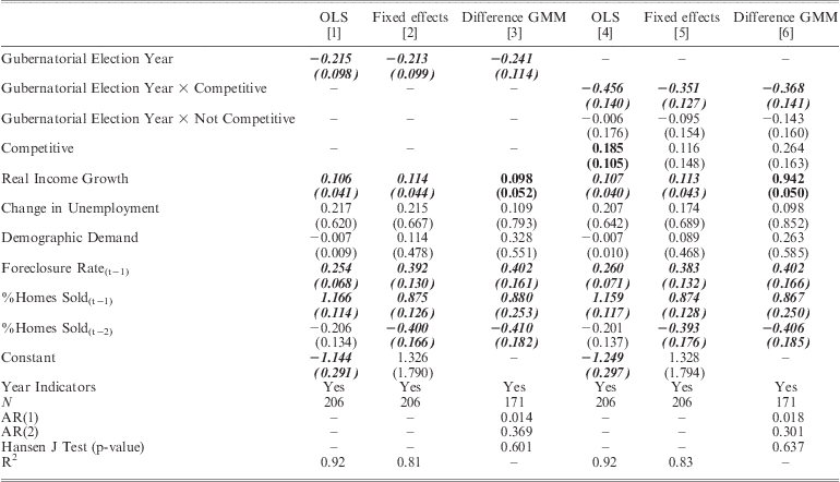
Across the various specifications, analysis of the home sales data suggests that the first and second lags of the dependent variable have significant effects, while additional lags do not; we accordingly estimate models that include two lags. We begin by presenting the results from OLS with standard errors clustered by state (and excluding the fixed effects), fixed effects with robust standard errors and difference-GMM with robust standard errors. The difference-GMM results are from one-step estimation, and the instruments for the endogenous variables include the second through fifth lags of %Homes Sold. Specification testing also suggests that the economic controls for income and unemployment are predetermined. Consistent with difference-GMM procedures for predetermined variables, they are instrumented with their first lags.Footnote 58 If income and unemployment are considered exogenous the substantive results are identical, but specification tests suggest that the model is overidentified; these results are available upon request. Table 6 presents the main findings.
Analysis of Pre-election Decline and Electoral Competitiveness Predictions, Home Sales Data
Note: Coefficients given above standard errors. Dependent variable equals %Homes Sold. In difference-GMM, the instruments for the lagged dependent variables include their second through fifth lags and the instruments for the predetermined economic controls include their first lags. All analyses conducted using STATA, which differences out the constant term in difference-GMM estimation. Estimates in bold significant at p < 0.1 (two-tailed) and estimates in bold italics significant at p < 0.05 (two-tailed).
Columns 1, 2 and 3 concern the Pre-election Decline Prediction, and Columns 4, 5 and 6 depict the results of the Electoral Competitiveness Prediction. The estimates in the first three columns suggest that the average effect of a gubernatorial election is to depress home sales significantly in the pre-election period. In all of the specifications, the coefficient on Gubernatorial Election Year is negative and significant at p < 0.05, two-tailed.
The magnitude of this effect is remarkably similar across the different estimators. In each case, the percentage of homes sold (out of all homes in the area, regardless of whether they are explicitly on the market) drops between two- and three-tenths of a percentage point. This impact is comparable to that of a standard deviation decrease in per capita income growth, which is 2.471 percentage points; such a change also produces a decline of two- to three-tenths of a percentage point in the percentage of homes sold (for example, in Column 1: 0.106 × 2.471 = 0.262). Thus the size of the electoral effect is similar to that of other, well-established influences on housing markets.
Columns 4 through 6 indicate that this impact is driven by competitive elections. The coefficients on Competitive × Gubernatorial Election Year suggest that the percentage of homes sold, out of all homes in the state, drops between one-third and one-half of a percentage point when the race is competitive. By comparison, the estimates on Not Competitive × Gubernatorial Election Year suggest a decline of one-tenth of a percentage point when one candidate leads by more than 5 percentage points of the vote. In addition, the estimates for the competitive elections are significant at p < 0.05, two-tailed, while those for the uncompetitive elections are not significant.
In each of the difference-GMM analyses in Table 6, the Hansen J-statistic indicates that the model is not overidentified. David Roodman argues that p-values below or even as great as 0.25 ‘should be viewed with concern’, while ones equal to 1.00 are a ‘classic sign’ that instrument proliferation has vitiated the capacity of the test to detect an overidentified model.Footnote 59 Neither Hansen J-statistic in Table 6 suggests cause for concern. The tests for serial correlation also support the models. First-order serial correlation is expected in difference-GMM analyses because the first differencing creates first-order serial correlation even when the errors in the original equation are independently and identically distributed. Second-order serial correlation should not be present, however, and as Table 6 shows, there is no evidence of it. We have also analysed models that restrict the instruments for the endogenous (lagged dependent) variables to the second through fourth lags and, separately, the third through fifth lags. In each case, specification testing supports the model and the theoretical predictions are substantiated at conventional significance levels.Footnote 60
Additional analysis, which is presented in the web appendix, indicates that the substantive findings are supported by system-GMM analyses, although specification tests reject these models. Specifically, if system-GMM is applied to the same instrument structure adopted for difference-GMM, the Hansen J-statistics and Difference-in-Hansen tests suggest an overidentified model.Footnote 61 We additionally analysed a battery of system-GMM models that reduced the instrument count; the results of these alternative models were similar – the substantive results held, but the Hansen tests suggested the models were overidentified.Footnote 62
The results for the control variables presented no major surprises, as indicated by Table 6. Home sales increase with real income. They are also positively associated with foreclosures; after a property forecloses, banks tend to sell it (at a substantially reduced price). The insignificance of the demographic estimates is consistent with some previous research.Footnote 63 Moreover, this insignificance (and that for unemployment) may relate to the fact that prior work has generally examined the determinants of home prices rather than sales.
In sum, the analysis of home sales provides substantial support for the Pre-election Decline and Electoral Competitiveness Predictions. Even accounting for a variety of economic and other determinants of housing markets, housing market activity is associated with a pre-election decline. Moreover, this overall effect appears to be driven by the competitive elections in which no candidate receives more than 55 per cent of the vote.
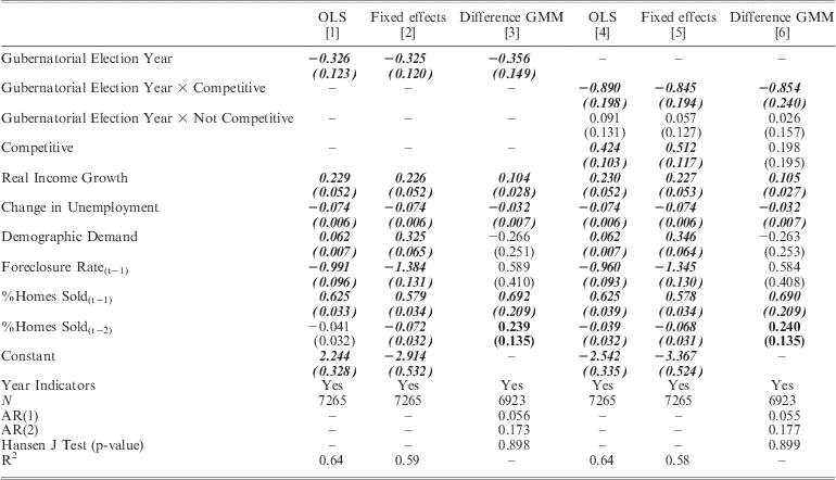
Table 7 shows that these results extend to home prices. As with the analysis of home sales, we begin by focusing on the results from the OLS, fixed-effects and difference-GMM models.
Analysis of Pre-election Decline and Electoral Competitiveness Predictions, Home Price Data
Note: Coefficients given above standard errors. Dependent variable equals %Change in Real Home Prices. In difference-GMM, the instruments for the lagged dependent variables include the third through fifth lags, collapsed. All analyses conducted with STATA, which differences out the constant term in difference-GMM estimation. Estimates in bold significant at p < 0.1, two-tailed, and estimate in bold italics significant at p < 0.05, two-tailed.
Columns 1, 2 and 3 estimate the average impact of a gubernatorial election. In all models the coefficient on Gubernatorial Election Year is significant (p < 0.05, two-tailed). In the year before an election, average home prices decline. Moreover, the size of the impact is relatively consistent across the disparate specifications. In each of the first three columns, prices fall by approximately one-third of a percentage point that year.
As with the home sales data, this effect appears to be driven largely by the competitive elections, in which the winner received less than 55 per cent of the vote. Columns 4, 5 and 6 suggest that when the candidates are within 5 percentage points of each other, home prices drop nine-tenths of a percentage point (p < 0.05, two-tailed). By comparison, when the election is relatively uncompetitive, there is no substantial drop in home prices. The coefficient on Gubernatorial Election Year × Not Competitive is even positive in some of the specifications, although in these cases it is small and not at all statistically significant.
The results for the other coefficients in Table 7 largely agree with expectations. Across all of the models, higher home prices are associated with increases in real income and decreases in unemployment. Also, in the OLS and fixed-effects specifications, the effects of foreclosures and demographic demand are in the expected direction and statistically significant. In the GMM models, these two control variables are not in the anticipated direction, but the effects are not at all significant.
The price data involve a substantially longer time series than the home sales data, and thus for the difference-GMM models a more restrictive instrument set is required to avoid overidentification. The instruments for the endogenous variables include the third through fifth lags, and these instruments are collapsed as described by Thorsten Beck and Ross Levine and by Roodman.Footnote 64 Specification testing suggests that the economic controls are not predetermined in these models, and therefore the variables are considered exogenous; however, if instead they are considered predetermined and the instruments include the first lag collapsed, the key coefficients remain significant at conventional levels, the magnitudes of these coefficients are similar and the Hansen J-statistics suggest that the models are not overidentified. The results are also robust to alternative sets of instruments for the lagged dependent variables, including the collapsed third and fourth lags or the collapsed second through fourth lags.Footnote 65 Finally, we assessed the appropriateness of system-GMM models with the home price data. Under any specification attempted (including ones that severely restricted the number of instruments) the substantive results held, yet the Hansen tests suggested the models were overidentified.Footnote 66
In sum, the findings on home prices corroborate those on home sales. The Pre-Election Decline and Electoral Competitiveness Predictions receive support with each dataset. On average the pre-election period is associated with a decline in home sales and prices. Furthermore, when the effects are analysed separately for competitive versus uncompetitive elections, it becomes clear that the average effect is driven by the highly competitive races. The housing market analysis thus provides substantial support for the Electoral Investment Theory.
Conclusion
We have argued that sectors of irreversible investments experience a pre-election decline due to the policy uncertainty generated by elections. Moreover, because policy uncertainty is associated with the competitiveness of the race and the policy differences between candidates/parties, the pre-election decline depends on these factors. The paper has conducted a variety of tests of the predictions, including analyses of individual-level survey data and aggregate housing market data. The results have provided substantial support for the predictions.
Additionally, the findings offer a possible reason that studies of opportunistic political business cycles have generally uncovered little evidence that economic growth within Organisation for Economic Co-operation and Development countries follows such cycles.Footnote 67 In particular, the results suggest that at least certain sectors of irreversible investment experience a decline at precisely the same time that opportunistic theories predict governments are simulating short-term expansions. Accordingly, future research might investigate whether theories of opportunistic cycles receive greater support if irreversible investment is separated from output.
The findings also suggest directions for future research. Most naturally, studies might examine whether the patterns observed in this paper extend to business investment or consumer durables such as automobiles. Additionally, future work should analyse whether the relationship among irreversible investments, elections and uncertainty holds in countries other than the United States. The endogenous nature of elections in many nations would necessitate additional theorizing about the precise relationship between the timing of elections and economic performance, but the arguments are broadly relevant to democratic nations.