


1 Introduction
Non-parametric and semi-parametric regression models are routinely used in comparative analyses to explore the dynamics shaping outcomes for countries, organizations and other similar units of analysis, and hazard models are among the most frequently employed. Hazard models analyze the time until an event occurs, allowing researchers to assess the factors that influence this duration (Box-Steffensmeier and Zorn Reference Box-Steffensmeier and Zorn2001; Cox Reference Cox1972; Yamaguchi Reference Yamaguchi2012). Applications include the onset of armed conflicts and mass atrocities (Cunningham, Gleditsch, and Salehyan Reference Cunningham, Gleditsch and Salehyan2009; Narang Reference Narang2014; Wayman and Tago Reference Wayman and Tago2010), withdrawal from international coalitions (Tago Reference Tago2009), the uneven application of the death penalty (Baumgartner et al. Reference Baumgartner, Box-Steffensmeier, Campbell, Caron and Sherman2020), and parliamentary dissolution (Strøm and Swindle Reference Strøm and Swindle2002), among others.
Despite their utility, and like other classes of regression models, there are unique challenges associated with applying hazard models for the purposes of comparative political analysis. These challenges stem from the fact that researchers routinely rely on data that represent the entire population or a sample of non-exchangeable observations (e.g., Cunningham et al. Reference Cunningham, Gleditsch and Salehyan2009; Kadivar Reference Kadivar2018; Strøm and Swindle Reference Strøm and Swindle2002; Tago Reference Tago2009). Such data violate basic distributional assumptions of generalized linear models (Belsley, Kuh, and Welsch Reference Belsley, Kuh and Welsch2004), increasing the likelihood that results mask substantively meaningful heterogeneity (Rambotti and Breiger Reference Rambotti and Breiger2020; Schoon, Melamed, and Breiger Reference Schoon, Melamed and Breiger2024b). This limitation has important implications for interpreting model results: when data are not representative of a known population, researchers cannot draw inferences about population-level trends. Instead, analyses are typically used to draw conclusions about the observed cases in the dataset (see, e.g., Seawright Reference Seawright2016). However, the degree to which the results apply to particular cases is masked by the model itself (Shalev Reference Shalev2007). Consequently, researchers must assume that the same conditions associated with, for example, armed conflict onset in Israel are equally relevant to armed conflict onset in the Congo or Ukraine.
Here, we describe and advance a set of methods referred to as Regression Inside Out (RIO), which stand to address these challenges (Schoon et al. Reference Schoon, Melamed and Breiger2024b; see also Breiger et al. Reference Breiger, Ackerman, Asal, David Melamed, Rethemeyer, Schoon, Salerno, Yang, Nau and Chai2011; Breiger and Melamed Reference Breiger and Melamed2014; Breiger, Lomi, and Pallotti Reference Breiger, Lomi and Pallotti2025; Melamed et al. Reference Melamed, Schoon, Breiger, Asal, Rethemeyer, Yang, Greenberg and Endsley2012; Melamed, Breiger, and Schoon Reference Melamed, Breiger and Schoon2013; Rambotti and Breiger Reference Rambotti and Breiger2020). RIO does this in three ways. First, it allows researchers to identify each individual observation’s additive contribution to the overall regression coefficient and variance (coefficient decomposition and variance decomposition), providing a methodology for empirically assessing which cases drive the aggregate findings rather than forcing assumptions of uniform relevance. Second, it allows researchers to visually map the regression model space, shifting from an exclusive analytic focus on population-level inferences and toward transparent, case-specific conclusions. Third, it allows researchers to geometrically analyze the relationships between both cases and variables, providing a framework for situating and evaluating the role of non-exchangeable observations in the context of generalized linear models.
Like well-established methods for regression diagnostics, RIO can identify unusual (i.e., high leverage and influential) observations. However, while diagnostic methods operate under the assumption that the overall data meet the basic distributional requirements for a regression model, RIO makes no such assumption. This makes it possible to identify distinct substantive patterns and discontinuities within subsets of data that might otherwise be masked by the net effect. This facilitates the kind of direct dialogue between substantive case-level insights and the output of the regression model that is critical to making credible claims about cases via the conditional distributions of variables. While diagnostic methods (e.g., DFBETA) identify how models change when individual cases are removed, RIO dually illustrates how the cases are related to each other, and how they are related to the variables within the field of the model at hand.
While RIO has the potential to address the challenges of applying hazard models in comparative political analysis, to date, it has not been adapted for use with these kinds of models. As such, in this article, we introduce a novel generalization of RIO that allows it to be used with any model in which linear predictors are estimated.Footnote 1 While RIO offers tools for uncovering the kinds of case-oriented insights that often motivate the use of non-parametric models, it has previously only been generalized to a limited number of generalized linear models. We also make two additional methodological contributions. First, while existing work on RIO outlines two approaches to decomposing variance, both have non-trivial limitations (discussed below). As such, we also introduce a bootstrap approach specifically adapted to RIO that distinguishes signal from noise in both the individual and aggregate contributions to the regression coefficients of observations. Second, we show how RIO is related to the closest diagnostic measure, DFBETA, and highlight differences between their results.
We begin with a brief introduction to RIO. Along with this overview, in Appendix A of the Supplementary Material, we provide a more detailed methodological introduction to RIO with a short example using ordinary least squares (OLS) regression. In this same appendix of the Supplementary Material, we also explain the mathematical relationship between RIO and DFBETA, the closest regression diagnostic, which we discuss below. After introducing RIO, we present our novel generalization, as well as the bootstrap approach. We then illustrate the utility of these methodological contributions through re-analyses of a recently published proportional hazard model examining the conditions leading to democratic failure (Kadivar Reference Kadivar2022).
2 Regression Inside Out: A brief introduction
RIO includes several related methods for examining, post-estimation, the aggregations and dual relationships between cases and variables that are masked at the level of regression coefficients. Here, we focus on three key features. The first is the coefficient decomposition, which allows analysts to compute each observation’s additive contribution to each estimated regression coefficient. The second is variance decomposition, which allows analysts to compute each observation’s contribution to the error variance and can flag cases that have a disproportionate impact on the model or draw attention to parts of the sample space. The third is model visualization, which allows analysts to project the cases and the variables into the same space, maintaining the relationships embedded in the regression coefficients while illustrating where and how the cases fit into the relationships between variables.
Regarding regression coefficient decomposition, Equation (1) presents the familiar OLS estimator with one adjustment. Rather than post-multiply by the outcome variable as a vector, we post-multiply by the outcome as a diagonal matrix. While the traditional estimator returns a p × 1 vector of regression coefficients, where p refers to the number of estimated parameters, Equation (1) returns a p × n matrix, where n refers to the sample size and columns present each observation’s contribution to the regression coefficients such that each row sums to an estimated regression coefficient. Sums of rows within selected sets of columns can reveal how subsets of cases contribute to the overall model coefficients (for additional details and an example, see Appendix A of the Supplementary Material):

In terms of variance decomposition, there are two existing techniques within the RIO suite of methods. The first is to decompose the model error variance, while the second uses a jackknife approach to investigate changes in the model standard errors (Schoon et al. Reference Schoon, Melamed, Breiger and Yoon2024a). While both approaches offer valuable insights, they both have meaningful limitations. Decomposition of the model variance does not translate to case-level standard errors as the variance and standard error are not linearly related. As such, this provides only a general approximation of the uncertainty that most analysts are interested in when it comes to computing a regression model. In contrast, the jackknife approach provides direct insights into the case-level standard errors. However, this approach requires a series of additional models with different sample spaces, systematically removing one case at a time and inspecting how the model standard errors change. As such, these case-level contributions are inconsistent with the case-level contributions obtained for the coefficients themselves, which can simply be summed to recover the overall model coefficients.
As we illustrate below, a core feature of RIO is the capacity to visualize the model space, allowing analysts to assess the relationships among cases and variables within the model. This visualization applies a singular value decomposition (SVD) to the matrix of predictor variables with the linear predictors appended to it. The linear relationship between the independent variables and the linear predictors is maintained across the dimensions of the SVD, and therefore, the leading dimensions of the SVD may be plotted for a model visualization that is like a correspondence analysis except that an explicit dependent variable has been specified (Breiger and Melamed Reference Breiger and Melamed2014). Likewise, the coefficient decomposition yields vectors of effects on the outcome which can be predicted by other variables to assess moderation and inductively discover statistical interaction effects (Schoon et al. Reference Schoon, Melamed and Breiger2024b, Chapter 6).
These features of RIO have a variety of applications. As detailed by Schoon et al. (Reference Schoon, Melamed and Breiger2024b), one natural use for RIO is to inductively identify interaction effects or other non-linearities in the sample space. Additionally, these authors illustrate how RIO can be used to capture the kinds of complexity that configurational comparative methods like qualitative comparative analysis (QCA) are commonly used to model (e.g., equifinality, multifinality and asymmetric causality; Ragin Reference Ragin2014; Schneider Reference Schneider2018; Schneider and Wagemann Reference Schneider and Wagemann2012), but in the context of a regression model that captures the probability patterns that QCA is not designed to account for (see, e.g., Braumoeller Reference Braumoeller2015; Hug Reference Hug2013). RIO also provides a critical resource for multi-method research, allowing analysts not only to identify statistically typical, deviant or extreme cases (among other types; Gerring and Cojocaru Reference Gerring and Cojocaru2016), but allowing researchers to identify the relationship between a substantively important case and all other cases in the regression model (for detailed elaboration on these and other applications, see Schoon et al. Reference Schoon, Melamed and Breiger2024b).
3 Methodological extensions
3.1 Generalizing Regression Inside Out
While RIO advances analyses aimed at making claims about observed cases (rather than a larger, unobserved population), to date it has been adapted for use only with parametric models, including OLS, logistic, Poisson, negative binomial and random intercept regression models (Schoon et al. Reference Schoon, Melamed and Breiger2024b). Yet, in contemporary political analysis, non- and semi-parametric models specifically adapted to modeling event occurrence are central to many areas of study. To remedy this mismatch, we introduce a generalization of RIO that facilitates coefficient decomposition and model visualization for any regression model that generates linear predictors. We also introduce a bootstrap procedure that allows us to assess whether case contributions differ from the average contribution, advancing prior efforts at variance decomposition, and detail the relationship between RIO and DFBETA.
Our generalization for the coefficient decomposition rests on a statistical identity, namely, that the predictor variables are, by definition, linearly related to the linear predictors from that model. Often those linear predictors are transformed to some other metric, such as predicted probabilities in the case of logistic regression. But the linear predictors are linearly related to the predictor variables and this forms the basis for our generalization: any model for which linear predictors exist can be decomposed by regressing the linear predictors on the independent variable matrix. This yields the same regression coefficients as the original non-OLS model and may be linearly decomposed in a way that weighted regressions (e.g., hazard models) cannot. Thus, the regression coefficients for any model with linear predictors can be decomposed into case contributions to the overall regression coefficients.Footnote 2 Likewise, by using the linear predictors in the model visualization, the relationships embedded in the regression model are recovered by the SVD.
3.2 A bootstrap approach for measuring uncertainty
To account for a case-level approach to uncertainty that is scalable from one case to an entire data set, we also developed a bootstrapping procedure adapted specifically for RIO. The procedure entails sampling cases with replacement, estimating the regression model for each such resampling, retaining the computed decomposition of each coefficient, repeating this process many times (we use 10,000 iterations) and computing the confidence interval from the distribution of regression contributions. Here, the reference point is the average contribution across cases or subsets thereof. In the context of hazard models, we extend this basic bootstrapping setup to account for the fact that cases have multiple observations through time. The purpose of this procedure is to distinguish the signal from noise of regression contributions. In contexts of non-exchangeable observations (such as countries), we conceive of estimates of uncertainty as quantifying noise in the data generating process (King, Keohane, and Verba Reference King, Keohane and Verba1994). In this view, the bootstrapped standard errors quantify the noise in an observation’s contribution to the regression coefficient in the sense that historical contingencies or stochastic processes giving rise to the observation may be different in different data generating regimes. Put differently, historical contingencies shape the observed data, potentially resulting in alternative realizations, and our estimates quantify the uncertainty of those contingencies (Berk, Western, and Weiss Reference Berk, Western and Weiss1995).
3.3 RIO’s relation to DFBETA
Practitioners might reasonably question the benefits of RIO relative to more conventional regression methods, particularly methods for regression diagnostics such as DFBETA. The precise relationship between these two methods has never previously been articulated. In Appendix A of the Supplementary Material, we provide a detailed explanation of the relationship between RIO and DFBETA along with an example. To briefly summarize, DFBETA is a derivative of RIO: it is equivalent to the difference between two RIO decompositions (one using the observed response and one using the linear predictors) normalized by the leverage of the case. This distinction is of great practical significance for interrogating regression models. As illustrated in the Supplementary Material, two cases may have large, opposing DFBETA values that suggest they cancel each other out in terms of influence on the final coefficient. However, RIO allows us to assess whether both cases provide substantial, same-signed contributions to the substantive effect that is measured by the model regression coefficient. By shifting the focus from how the model changes in a counterfactual state (case removal) to how the model is constructed in its actual state, RIO enables researchers to understand the empirical “why” behind their results rather than simply flagging problematic outliers.
4 Illustration: Durable democracy and non-violent mobilizationFootnote 3
To illustrate these generalizations of RIO, we replicate and re-analyze a published example of a Cox proportional hazard model. In his book, Popular Politics and the Path to Durable Democracy, Kadivar (Reference Kadivar2022) examines the conditions that shape the durability of democratic regimes, presenting compelling evidence that prolonged, grassroots mobilization is the foundation for establishing an enduring democracy. The book presents both statistical analyses of a novel dataset and in-depth case studies to explore the mechanisms linking popular mobilization and democratic durability. Building on his analyses, we turn Kadivar’s Cox proportional hazard model inside out and explore the results in dialogue with his incisive historical research.
The dependent variable in the hazard model we replicate is democratic failure, which is present when “executive power is achieved through means other than reasonably competitive elections” (p. 29). The unit of time is years, beginning with a country’s democratic transition (for countries that transitioned to electoral democracy post-1950), ending with democratic failure or censoring if still a democracy by the end of the study period (2010).Footnote 4 There are 115 electoral democracies that fit this criterion, of which 112 (across 80 countries) have full socio-economic data, and this is the population used in the analysis to follow. The primary independent variable is “duration of [unarmed] popular campaigns contributing to a democratic transition” (p.30). The controls are the duration of armed campaigns, GDP per capita (ln), GDP growth, population (ln) and past democratic experience. Kadivar finds that the length of unarmed popular campaigns is positively associated with the survival of electoral democracies, concluding that “pessimistic views about the negative repercussions of mass mobilization for democratic durability are wrong” (p.35).
Kadivar presents in-depth studies of three cases: South Africa from 1994 to present, Poland from 1989 to present and Pakistan from 1988 to 1999. He notes that South Africa and Poland are paradigmatic cases because they witnessed the most protracted mobilization campaigns in the dataset. Moreover, within the bounds of the study, neither experienced democratic failure. Pakistan similarly aligns with this theorizing but exhibits the inverse characteristics of the other two cases, as democratization was driven by elites rather than popular pressure, seeding the ground for its democratic failure. Kadivar’s analysis of these cases gives us a useful point of reference for exploring the role of cases within the regression model.
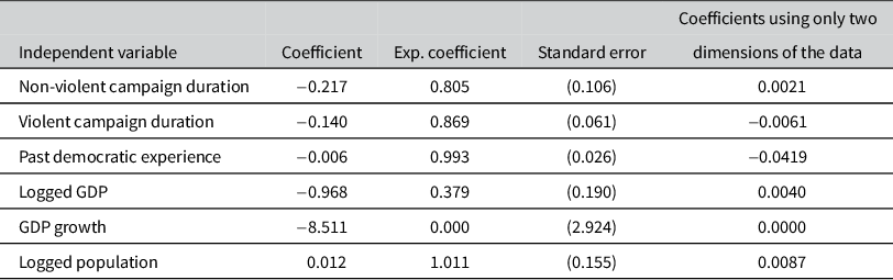
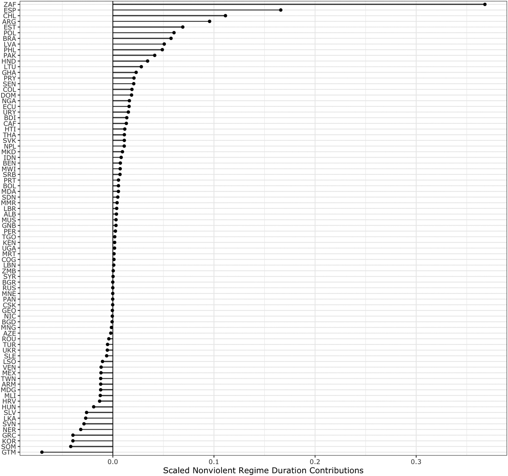
Table 1 presents our replication of Kadivar’s original analysis,Footnote 5 and Figure 1 plots the cases’ contributions (summed by country and then scaled by the overall sum, and ranked by most positive to most negative) to the key independent variable: non-violent campaign duration. Here, values greater than 0 indicate the contribution of this country is in the same direction as the main model coefficient. What should be immediately evident in Figure 1 is that South Africa (ZAF) disproportionately contributes to the overall regression coefficient. This is not surprising. In presenting the raw data, Kadivar (Reference Kadivar2022, Reference Schneider and Wagemann27–Reference Schneider28) shows that South Africa stands out for having unarmed mobilization with nearly twice the duration of the next highest-ranked country (13 years as compared to 8 in Bolivia) and more than six times the average (mean = 1.968). Consistent with the logic underlying Kadivar’s case selection, Poland (POL) and Pakistan (PAK) similarly make large positive contributions to the overall regression coefficients. While many of the cases in Figure 1 align with this theorizing, there are several that do not (e.g., they have contributions that are the inverse of the direction of the main model coefficient). In this context, the cases that have strong negative contributions are possible negative cases that challenge the theorized relationship (see Emigh Reference Emigh1997; Gerring and Cojocaru Reference Gerring and Cojocaru2016). One notable case not discussed in detail by Kadivar is Guatemala (GTM), which has a large attenuating effect on the overall regression coefficient. Kadivar (Reference Kadivar2022, 142, n. 29) indeed notes that Guatemala presents “the longest case of civil war in [his] analysis” and that the leading opposition group “did transform into a political party.” While he notes that this party “has not been an important actor in Guatemalan elections, not even as a serious opposition party,” disjuncture between democratic durability and mobilization supports our nomination of Guatemala as a potential negative case with respect to Kadivar’s main thesis. We revisit Guatemala below.
Replication of Table 5, Model 1, in Kadivar (Reference Kadivar2022).

Table 1. Long description
The table consists of five columns: Independent variable, Coefficient, Exp. coefficient, Standard error, and Coefficients using only two dimensions of the data.
* Non-violent campaign duration: Coefficient -0.217, Exp. coefficient 0.805, Standard error 0.106, Two-dimension coefficient 0.0021.
* Violent campaign duration: Coefficient -0.140, Exp. coefficient 0.869, Standard error 0.061, Two-dimension coefficient -0.0061.
* Past democratic experience: Coefficient -0.006, Exp. coefficient 0.993, Standard error 0.026, Two-dimension coefficient -0.0419.
* Logged G D P: Coefficient -0.968, Exp. coefficient 0.379, Standard error 0.190, Two-dimension coefficient 0.0040.
* G D P growth: Coefficient -8.511, Exp. coefficient 0.000, Standard error 2.924, Two-dimension coefficient 0.0000.
* Logged population: Coefficient 0.012, Exp. coefficient 1.011, Standard error 0.155, Two-dimension coefficient 0.0087.
Case contributions to the estimated effect of non-violent campaign duration.

Figure 1. Long description
The horizontal dot plot features a vertical axis on the left listing three-letter country codes and a horizontal axis at the bottom labeled Scaled Nonviolent Regime Duration Contributions. The x-axis ranges from approximately negative 0.1 to 0.4 with major grid lines at 0.0, 0.1, 0.2, and 0.3. A bold vertical baseline is set at 0.0.
Data points are represented by black dots connected to the 0.0 baseline by horizontal lines. The countries are ordered from top to bottom by their contribution value.
* At the top, Z A F shows the highest positive contribution, extending past 0.35.
* Other high positive contributors include E S P, C H L, A R G, and E S T, with values between 0.1 and 0.2.
* A large cluster of countries, starting from P O L down through C O G, show small positive contributions that gradually decrease toward zero.
* Several countries including L B N, Z M B, and S Y R are positioned exactly or nearly on the 0.0 baseline.
* Starting from A Z E and moving downward, countries show increasingly negative contributions.
* The bottom of the list features G T M with the most significant negative contribution, followed by S O M, K O R, and G R C, all falling between 0.0 and negative 0.1.
These results offer useful insights into how each country influences the coefficient for the key independent variable. Kadivar’s identification of South Africa and Poland as paradigmatic cases is clearly reflected in the results of the decomposition. Similarly, Pakistan’s positive contribution reflects the correlation between democratic failure and non-violent mobilization.
4.1 Visualizing the model space
We explore the above insights further by plotting the overall regression space. Exploiting the linear relationship between linear predictors and independent variables, this visualization maintains the association between the predictors and the outcome. By appending the linear predictors to the matrix of independent variables, and then taking the SVD of this matrix, the leading dimensions from the row and column space matrices of the SVD provide dimensional scores that, when plotted, yield an image of the model maintaining the observed associations. The result is akin to a correspondence analysis because the linear relationships between predictors and the outcome is maintained (Greenacre Reference Greenacre2017). However, unlike a correspondence analysis, this plot has an explicit outcome (Breiger Reference Breiger2009; Schoon et al. Reference Schoon, Melamed and Breiger2024b).
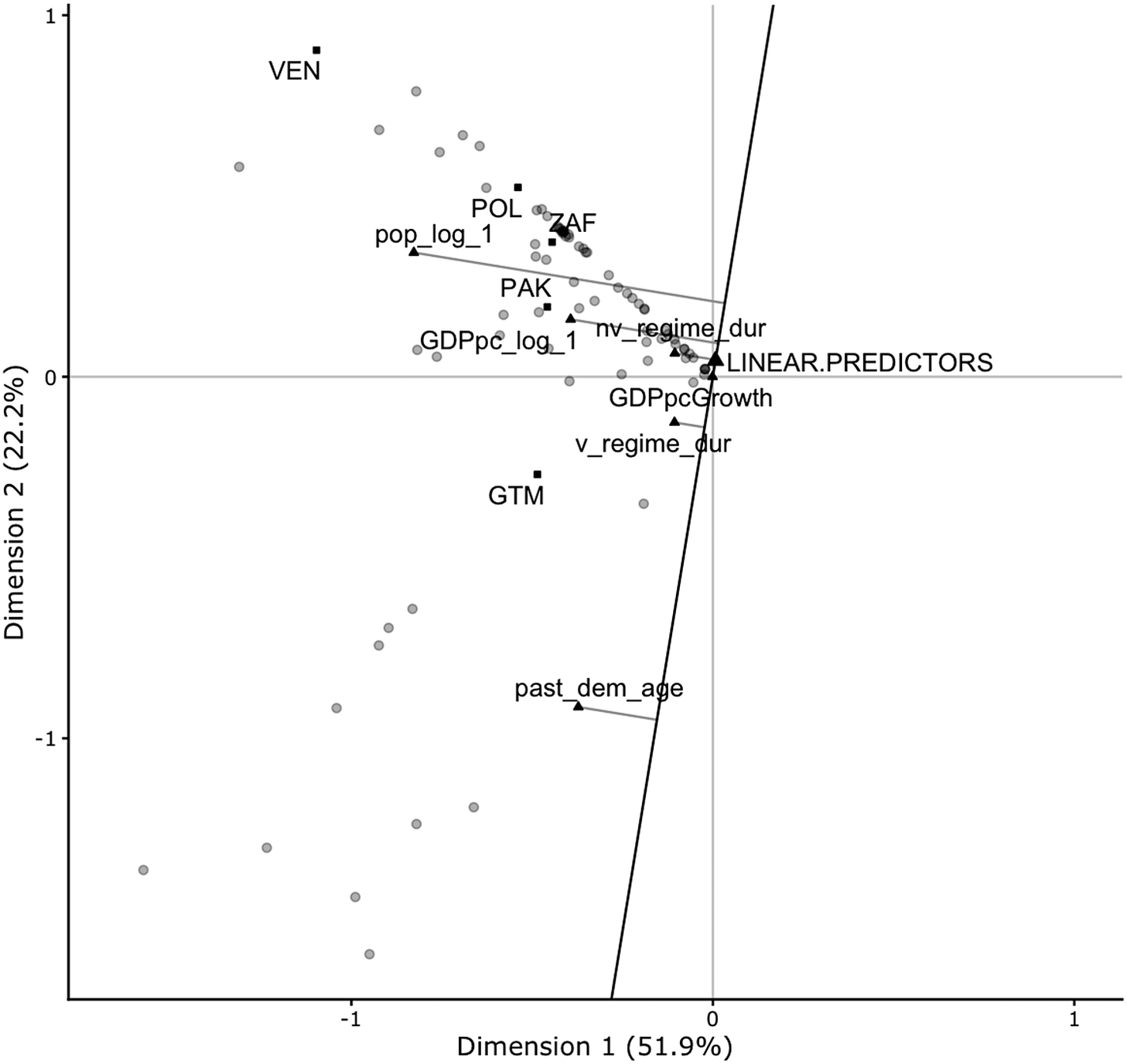
Figure 2 uses the methods described above to plot the model space with all cases and variables. In this plot, gray dots represent cases (i.e., countries, with contributions averaged across all country-years) and variables are indicated by black triangles. Five cases—Guatemala (GTM), Pakistan (PAK), Poland (POL), South Africa (ZAF) and Venezuela (VEN)—are labeled and singled out using black squares. The greater a case’s proximity to a variable in the plot, the greater the intensity of their association. Lines are projected from each independent variable at right angles to a line connecting the “LINEAR.PREDICTOR” to the origin. These projections aid in interpretation, allowing the net effects of the variables to be interpreted geometrically. The distance between the origin and the point where the projection from each variable intersects the line is proportional to the two-dimensional version of the regression coefficient for that variable. This is because proportionality is constrained by the dimensionality of the model. In this case, the linear predictors are appended to six independent variables. We plot the leading two dimensions, which account for 74.1% of the variation in the data (see Figure 1; dimension 1 is 51.9% and dimension 2 is 22.2%). Table 1 also presents the two-dimensional version of the regression coefficients for transparency.Footnote 6 Taken together, this figure provides the best (in the sense of least-squares) two-dimensional visualization of the model space.
RIO visualization of the hazard model in Table 1.

Figure 2. Long description
A biplot with Dimension 1 on the horizontal axis (51.9 percent) and Dimension 2 on the vertical axis (22.2 percent). The axes range from -1 to 1.
Data Distribution:
* Top-Left Quadrant: Contains a high density of grey circular data points and specific country markers including V E N (highest on Dimension 2), P O L, and P A K.
* Top-Right Quadrant: Contains Z A F and a cluster of points near the origin.
* Bottom-Left Quadrant: Contains G T M and several scattered grey points extending toward the bottom-left corner.
* Bottom-Right Quadrant: Mostly empty of country labels but contains the terminal ends of several predictor vectors.
Vectors and Predictors:
Several grey lines with triangular arrowheads originate from a central point labeled L I N E A R dot P R E D I C T O R S located near (0, 0.1).
* pop_log_1: Points toward the top-left (negative Dimension 1, positive Dimension 2).
* G D P p c_log_1: Points horizontally to the left.
* nv_regime_dur: Points slightly upward and left.
* G D P p c G r o w t h: Points slightly downward and left.
* v_regime_dur: Points downward into the bottom-right quadrant.
* past_dem_age: A long vector pointing steeply downward toward the bottom-center.
A thick black diagonal line bisects the right side of the plot, running from the bottom-center toward the top-right.
Through this figure, we can gain insights into the role that cases play in the model and the relationships among them in the model space. While Figure 1 shows that South Africa has a disproportionate contribution to the effect of non-violent mobilization, Figure 2 shows that it is very much in the middle of the overall regression space. This supports the assertion that it is, in fact, a paradigmatic case as Kadivar argues and not, as Figure 1 might suggest, anomalous.
The geometry of the plot allows us to assess the similarity between cases within the model space using cosine similarity. Similarity is a function of further distances from the origin at smaller angles (Goodman Reference Goodman1985). More acute angles are more similar, whereas right angles are orthogonal and obtuse angles indicate dissimilarity. Using that approach, it is visually evident that South Africa, Poland and Pakistan are quite similar. However, these three countries also have a high cosine similarity with Venezuela which, within the model space, is an outlying case. Exploring the raw data, we see that the reason for this is because Venezuela has the longest regime durability of any country in the dataset, but a history (albeit short) of non-violent mobilization and no history of violent mobilization in the dataset. Given these characteristics, Venezuela’s position in the plot suggests that it might be a valuable candidate for further investigation as it has the desired outcome but with a far lower degree of non-violent mobilization (the key hypothesized cause of regime durability) than the paradigmatic cases of South Africa or Poland.
Following from our discussion of Figure 1, we also highlight Guatemala in Figure 2. Figure 1 showed Guatemala having a strong attenuating effect on the overall regression coefficient for non-violent mobilization, and here, we see that it has a nearly orthogonal relationship to South Africa (i.e., it is at a nearly right angle when points are projected from each country to the origin). Digging into the data, we find that Guatemala had similar degrees of democratic durability to South Africa, but no non-violent mobilization and a long history of violent mobilization. This suggests that, like Venezuela, Guatemala might be a particularly informative case for exploring why there is democratic durability despite either a lack of extensive non-violent mobilization (as in Venezuela) or extensive violent mobilization. Appendix B of the Supplementary Material details these relationships further, highlighting the effect of non-violent campaign duration and the relationships between cases.
4.2 Bootstrapping the coefficient contributions
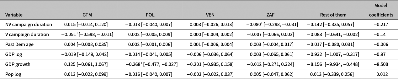
We further explore these cases in the context of the model by seeing how their numeric contributions compare to each other and to all other cases across all variables. Table 2 shows the decomposition of Model 1 from Table 5 of Kadivar (Reference Kadivar2022; the coefficients of our Table 1). We show the contributions of Guatemala, Poland, Venezuela, South Africa and the rest of the cases, along with the overall model coefficients (here, we do not exponentiate the coefficients). The contributions sum to the overall coefficient. This technique takes the estimated coefficient and decomposes it by cases or subsets of them (Schoon et al. Reference Schoon, Melamed, Breiger and Yoon2024). In addition to the decomposition, we also include the estimates from the inner 95% of the bootstrapping procedure discussed above. In this context of hazard models, the bootstrap entails: (i) taking a sample of size N from all N countries, with replacement, (ii) fit the hazard model on the sample, (iii) with the linear predictors from (ii), decompose the hazard coefficients using Equation (1), (iv) sum the rows (over time) by cases sampled in the bootstrap, (v) average over cases that were sampled multiple times to account for their presence multiple times, (vi) match the bootstrapped contributions to the observed ones, and (vii) sort the bootstrapped distributions to compute the 2.5 and 97.5 percentiles. Table 2 flags contributions where the inner 95% of the bootstrapped distribution does not contain zero. This signifies that the case contributes a substantial portion of the estimated regression coefficient, more so than the expectation of the regression coefficient divided by the number of cases.
Decomposition of Table 5, Model 1, in Kadivar (Reference Kadivar2022).

Table 2. Long description
The table consists of seven columns: Variable, G T M, P O L, V E N, Z A F, Rest of them, and Model coefficients.
* N V campaign duration: G T M 0.015 [-0.014, 0.120]; P O L -0.013 [-0.040, 0.007]; V E N 0.003 [-0.026, 0.013]; Z A F -0.080 super + [-0.288, -0.031]; Rest -0.142 [-0.335, 0.057]; Model -0.217.
* V campaign duration: G T M -0.051 super + [-0.598, -0.011]; P O L 0.002 [-0.005, 0.009]; V E N 0.000 [-0.004, 0.002]; Z A F -0.007 [-0.066, 0.002]; Rest -0.083 super + [-0.641, -0.002]; Model -0.14.
* Past Dem age: G T M 0.004 [-0.008, 0.035]; P O L 0.002 [-0.001, 0.006]; V E N 0.001 [-0.006, 0.004]; Z A F 0.003 [-0.004, 0.017]; Rest -0.017 [-0.080, 0.031]; Model -0.006.
* G D P log: G T M -0.019 [-0.149, 0.042]; P O L -0.014 [-0.041, 0.005]; V E N -0.006 [-0.036, 0.064]; Z A F 0.003 [-0.065, 0.061]; Rest -0.932 super + [-1.007, -0.317]; Model -0.97.
* G D P growth: G T M 0.125 [-0.061, 1.067]; P O L -0.268 super + [-0.477, -0.027]; V E N -0.201 [-0.935, 0.158]; Z A F -0.012 [-0.271, 0.324]; Rest -8.156 super + [-9.934, -0.448]; Model -8.508.
* Pop log: G T M 0.013 [-0.022, 0.099]; P O L -0.016 [-0.040, 0.007]; V E N -0.003 [-0.022, 0.037]; Z A F 0.005 [-0.047, 0.062]; Rest 0.013 [-0.339, 0.256]; Model 0.012.
Note: super + denotes that the bootstrapped 95 percent confidence interval does not contain zero.
Note: +Denotes that the bootstrapped confidence interval does not contain zero (95% confidence interval). Contributions to the estimated Cox hazard regression coefficients and [95% bootstrapped confidence intervals] shown (logged-hazard ratio). Full model coefficients shown in the final column.
Focusing on the cases where the bootstrapped confidence interval shows a non-zero contribution, we see that South Africa is a driving force behind the effect of non-violent campaign duration. Notably, the “Rest of Them” category does not appear to make a meaningful contribution (at least on average). Because Table 2 suggests that it is possible the effect is largely driven by South Africa, we assessed the possibility that South Africa is entirely driving the effect by dropping this case from the data and re-running the model. Consistent with the fact that most of the cases in the model align with Kadivar’s theorizing (as shown in Figure 1), the substantive conclusions were the same but the effects were attenuated. For its part, Guatemala is a driving force in the effect of violent campaign duration. Notably, however, the remaining cases also contribute meaningfully to this effect.Footnote 7 With the exception of Poland’s contribution to GDP growth, none of these cases appear to be unduly influencing any of the other effects in the model.
4.3 RIO’s relation to DFBETA
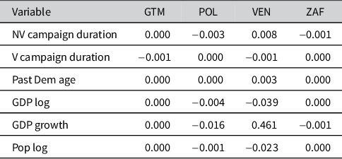
As noted above and formalized in Appendix A of the Supplementary Material, RIO is related to regression diagnostics. The closest existing diagnostic measure is DFBETA, which removes one case at a time to quantify how much each coefficient changes. Other diagnostics, such as Cook’s D, DFFITs or various forms of residuals, are case- or model-level diagnostics rather than coefficient-level diagnostics. While RIO formalizes and illustrates the relationships between the cases and the variables, DFBETA quantifies how much each coefficient changes when the relationships between a focal case and all other cases is removed from the model. To illustrate the difference between RIO and DBFETA in this context, Table 3 provides DFBETA for each of the four cases noted above, summed over the years they are observed in the data. Appendix C of the Supplementary Material describes how RIO is related to other standard diagnostics for hazard models and presents these results disaggregated by country-years.
Sum of DFBETA for each country-year.

Table 3. Long description
The table consists of five columns. The first column lists the variables, and the subsequent columns are headed by country initialisms: G T M, P O L, V E N, and Z A F.
* N V campaign duration: G T M 0.000, P O L minus 0.003, V E N 0.008, Z A F minus 0.001.
* V campaign duration: G T M minus 0.001, P O L 0.000, V E N minus 0.001, Z A F 0.000.
* Past Dem age: G T M 0.000, P O L 0.000, V E N 0.003, Z A F 0.000.
* G D P log: G T M 0.000, P O L minus 0.004, V E N minus 0.039, Z A F 0.000.
* G D P growth: G T M 0.000, P O L minus 0.016, V E N 0.461, Z A F minus 0.001.
* Pop log: G T M 0.000, P O L minus 0.001, V E N minus 0.023, Z A F 0.000.
Note: Selected countries shown.
Notably, RIO illustrates how South Africa, one of Kadivar’s paradigmatic cases, contributes to the negative net effect of non-violent campaign duration, while DFBETA shows a quite small effect from removing all country-years for South Africa (−0.001). Indeed, DFBETA, on the other hand, finds that Poland plays the largest role in altering the negative effect of non-violent campaign duration, while RIO suggests a modest role of Poland (less than that of South Africa, for example) in its additive contribution. As discussed in Appendix C of the Supplementary Material, both results noted here are consistent when we drill down and examine country-years. We also note a further advantage of a RIO-approach is that we can inspect not only how cases (and sets of cases) contribute to the overall regression coefficient, but also the significance of said contribution; to our knowledge, no comparable significance test exists for DFBETA diagnostics.
There are several takeaways from our re-analysis of Kadivar’s model. First, our findings support Kadivar’s substantive conclusion that South Africa is, in fact, a paradigmatic case. While it stands out in its effect on non-violent mobilization, it is otherwise not an outlier relative to other cases in the model. More broadly, though, using RIO helps us understand how South Africa as well as Poland and Pakistan fit within the overall model space and their relationship to other countries. In this context, we find that South Africa, Poland and Pakistan are excellent illustrations of Kadivar’s theory, but our findings also suggest that Venezuela and Guatemala might yield valuable insights that could extend his theorizing. While neither of these cases is flagged as substantively significant (and Kadivar does not analyze them in depth), their position within the overall model space highlights the potential value of digging deeper to understand the mechanisms driving regime durability.
5 Discussion
We generalized RIO (Schoon et al. Reference Schoon, Melamed and Breiger2024b) to any model for which linear predictors are estimated, and we illustrated this generalization in the context of Cox proportional hazard models. This provides a novel approach to identify and visualize the contributions to each of the coefficients, either by individual cases or subsets of them, in the context of one of the most widely-used models for comparative political analysis. We also articulated how RIO is related to regression diagnostics, particularly DFBETA. The introduction of a new bootstrapping procedure allowed us to distinguish significant case contributions from random noise, even when cases included repeated observations over time. In so doing, we have shown a valuable way for researchers to enhance interpretation and provide deeper insight into statistical results. As demonstrated, RIO assesses the contributions to a regression coefficient of case-level deviations (with respect to single cases as well as sets of cases), along with measures of significance that incorporate the bootstrapping approach presented in this article.
Our re-analysis of Kadivar’s (Reference Kadivar2022) hazard model demonstrated the utility of this generalized approach. Here, we found that individual countries such as South Africa and Guatemala disproportionately contribute to the effects of non-violent campaign duration. Bootstrapped confidence intervals confirmed the robustness of these findings. Our re-analysis highlights valuable opportunities for further empirical and theoretical development. What is it about certain countries that cluster together that unites them in a case-by-case sense, and how should we make sense of how these underlying relationships are shaping our scholarly understandings?
More broadly, our analyses demonstrate how RIO can contribute to a more holistic understanding of the inherent complexities underlying political processes. Though our example focuses on country-level studies, this method is particularly useful in any scenario where the cases have some meaningful interpretability in and of themselves (e.g., countries, groups and democratic systems), thus lending themselves to qualitative examination. Such further analyses could provide a richer picture of patterns so often used to infer relationships between variables—and, indeed, patterns that have been used to inform policy decisions. RIO shows clearly that, while model coefficients can provide useful insight in general, it is important to consider the consistency of specific cases “within” these coefficients.
RIO also provides a valuable foundation for engaging with large N studies and “big data.” In their essay on the role of regression in big data, Lee and Martin (Reference Lee and Martin2015) detail how the massive scale of big data undermines the value of statistical significance because nearly every correlation becomes significant in large samples. In this context, they propose a cartographical approach, using visualization to map how different subsets of data behave, treating outliers as meaningful sub-populations rather than individual errors to be discarded. RIO’s ability to visualize regression models supports such an approach via more conventional regression models, fostering dialogue between the two and enhancing our ability to engage with the breadth of information that big data affords.
Methodologically, while our focus was on a particular class of survival models, we have shown how this generalization of RIO can apply to any models for which linear predictors are obtainable. As such, this approach can be readily extended to other classes of survival models and the entirety of the generalized linear model. We consider this groundwork for future methodological innovations, offering new avenues to explore the complexities of social phenomena.
Acknowledgements
We thank Ali Kadivar for sharing his data and for valuable discussions.
Author contributions
D.M. and R.L.B. conceived the extensions presented in this article. All authors contributed equally to the analysis and to the writing.
Funding statement
We also gratefully acknowledge support from the Intelligence Advanced Research Projects Administration (IARPA; Award No. 171219000006) to D.M., E.W.S. and R.L.B.
Supplementary material
To view supplementary material for this article, please visit https://doi.org/10.1017/pan.2026.10056.



 Open access

