1 Introduction
In the past two decades, accumulated evidence has been presented to support the viewpoint that hairpin packets are a plausible model to account for the key structural and dynamical characteristics in the outer region of wall-bounded turbulence. This hairpin-packet model, as first suggested by Smith et al. (Reference Smith, Walker, Haidari and Sobrun1991) and Adrian, Meinhart & Tomkins (Reference Adrian, Meinhart and Tomkins2000), describes the streamwise alignment of individual hairpin-like vortices and their hierarchical organization into a coherent packet. One of the attractive values of this model is that it provides a possible mechanism for the growth of small-scale structures into larger structures (Natrajan & Christensen Reference Natrajan and Christensen2006; Hong et al. Reference Hong, Katz, Meneveau and Schultz2012).
1.1 Geometrical characteristics of the hairpin packets
The stereoscopic flow visualization performed by Delo, Kelso & Smits (Reference Delo, Kelso and Smits2004) provided a three-dimensional (3D) view of the hairpin-packet organization in a low-Reynolds-number (
 $Re$
) turbulent boundary layer. Stereo particle image velocimetry (PIV) measurements in the inclined spanwise–wall-normal planes by Hutchins, Hambleton & Marusic (Reference Hutchins, Hambleton and Marusic2005) revealed an instantaneous arrangement of multiple counter-rotating swirling patterns occupying the vertically aligned shear layers in the
 $135^{\circ }$
inclined plane, consistent with the cluster of hairpin legs/necks in the hairpin-packet model. Elsinga et al. (Reference Elsinga, Adrian, van Oudheusden and Scarano2010) took a tomographic PIV measurement to show the spatial organization of hairpin vortices in a high-
 $Re$
supersonic turbulent boundary layer. Dennis & Nickels (Reference Dennis and Nickels2011) further used high-speed cross-plane stereo PIV measurement together with Taylor’s frozen hypothesis to reconstruct a ‘quasi-instantaneous’ 3D pattern of the hairpin packets at moderate Reynolds number (
 $Re$
), which was recently validated by a moving tomographic PIV measurement (Gao, Ortiz-Duenas & Longmire Reference Gao, Ortiz-Duenas and Longmire2013).
Owing to the collective induction of both the spanwise-rotated heads and the streamwise-extended counter-rotating leg pairs of multiple hairpin vortices, a hairpin packet will leave a typical two-dimensional (2D) imprint in the streamwise–wall-normal plane, which is characterized as an interface that inclines away from the wall at an angle of
 $10^{\circ }{-}20^{\circ }$
and connects the neighbouring hairpin heads within the packet, as well as the underlying low-momentum large-scale motions (LSMs) whose streamwise coherence extends up to
 $(2{-}3)\unicode[STIX]{x1D6FF}$
(
 $\unicode[STIX]{x1D6FF}$
is the boundary layer thickness or the half channel/pipe height).
In low-to-moderate
 $Re$
scenarios, this planar imprint has been frequently observed in the outer region of wall-bounded turbulence over either a smooth wall (Adrian et al.
Reference Adrian, Meinhart and Tomkins2000; Natrajan & Christensen Reference Natrajan and Christensen2006), an irregular rough wall (Wu & Christensen Reference Wu and Christensen2010) or superhydrophobic surfaces (Tian et al.
Reference Tian, Zhang, Jiang and Yao2015). The typical planar Lagrangian coherent structures (LCS) measured by finite-time Lyapunov exponents (FTLEs) in both a low-
 $Re$
turbulent boundary layer (Pan, Wang & Zhang Reference Pan, Wang and Zhang2009) and a transitional boundary layer (Pan, Wang & He Reference Pan, Wang and He2012; He et al.
Reference He, Pan, Feng, Gao and Wang2016) are also consistent with it. The ramp-like turbulent bulges (Head & Bandyopadhyay Reference Head and Bandyopadhyay1981) have been attributed to those hairpin-packet imprints that occasionally penetrate into the outermost edge of the boundary layer (Adrian Reference Adrian2007). Additionally, the signature of the alignment/concatenation of either multiple hairpin packets, bulges or LSMs have been observed in high-
 $Re$
turbulence, ranging from boundary layer flow (Ganapathisubramani, Clemens & Dolling Reference Ganapathisubramani, Clemens and Dolling2006; Guala, Hommema & Adrian Reference Guala, Hommema and Adrian2006; Dennis & Nickels Reference Dennis and Nickels2011), channel/pipe flow (Kim & Adrian Reference Kim and Adrian1999; Baltzer, Adrian & Wu Reference Baltzer, Adrian and Wu2013; Dennis & Sogaro Reference Dennis and Sogaro2014; Hellström, Ganapathisubramani & Smits Reference Hellström, Ganapathisubramani and Smits2015; Hellström & Smits Reference Hellström and Smits2017) to atmosphere surface layer flow (Hutchins et al.
Reference Hutchins, Chauhan, Marusic, Monty and Klewicki2012; Wang & Zheng Reference Wang and Zheng2016). This offers a candidate explanation for the origin of very-large-scale motions (VLSMs) or superstructures.
Statistical evidence for the existence of hairpin packets was first obtained by Christensen & Adrian (Reference Christensen and Adrian2001). They used linear stochastic estimation (LSE) to estimate the conditional-averaged velocity field associated with one clockwise-rotated swirling event (or prograde vortex) in the streamwise–wall-normal plane. The resulting structure consists of a series of prograde vortices that are aligned in the streamwise direction and inclined away from the wall. This structure resembles the instantaneous hairpin-packet imprints, thus highlighting their prevalence and robustness for surviving the averaging operation. Christensen et al. (Reference Christensen, Wu, Adrian and Lai2004) further estimated the streamwise spacing of the neighbouring hairpin heads (prograde vortices) within a packet by the peak wavenumber of the streamwise spectrum of the Eulerian acceleration obtained via particle image accelerometry measurement. The mean spacing was found to be
 $(0.15{-}0.2)\unicode[STIX]{x1D6FF}$
at
 $Re_{\unicode[STIX]{x1D70F}}=550{-}1747$
(
 $Re_{\unicode[STIX]{x1D70F}}=\unicode[STIX]{x1D6FF}/l^{\ast }$
,
 $l^{\ast }=\unicode[STIX]{x1D708}/u_{\unicode[STIX]{x1D70F}}$
is the viscous length scale,
 $\unicode[STIX]{x1D708}$
is the kinematic viscosity, and
 $u_{\unicode[STIX]{x1D70F}}$
is the friction velocity), and the magnitude decreases with increasing
 $Re_{\unicode[STIX]{x1D70F}}$
if scaled by the outer unit
 $\unicode[STIX]{x1D6FF}$
.
The 3D velocity–vorticity correlation structures, as recently identified by Chen et al. (Reference Chen, Hussain, Pei and She2014) in a low-
 $Re$
turbulent channel flow, are geometrically similar to the hairpin-packet model. Nevertheless, the conditionally averaged 3D velocity field associated with a single spanwise swirling event in Dennis & Nickels (Reference Dennis and Nickels2011) only reveals one hairpin-like vortex striding above one low-speed LSM, in distinct contrast to the instantaneous pattern of multiple vortices with strong spatial coherence (see figures 18 and 6 in Dennis & Nickels (Reference Dennis and Nickels2011) for comparison). This reminds us to be cautious about interpreting the averaged structures subject to a simple condition, and poses the impetus for developing more sophisticated detection criteria for the investigation of vortex organization in a statistical sense.
1.2 Dynamical significance of the hairpin packets
The regular organization and spatial hierarchy of the hairpin-packet model is compatible with both the self-similar growth of the attached eddies in the attached-eddy hypothesis (Perry & Chong Reference Perry and Chong1982; Marusic & Perry Reference Marusic and Perry1995; Perry & Marusic Reference Perry and Marusic1995) and the parent–offspring regeneration scenario of individual hairpin vortices (Smith et al. Reference Smith, Walker, Haidari and Sobrun1991; Zhou et al. Reference Zhou, Adrian, Balachandar and Kendall1999; Kim, Sung & Adrian Reference Kim, Sung and Adrian2008). It is also favoured by streak instability theory, which predicts the generation of trains of hairpin vortices from the varicose breakdown of low-speed streaks (Asai, Minagawa & Nishioka Reference Asai, Minagawa and Nishioka2002; Brandt, Schlatter & Henningson Reference Brandt, Schlatter and Henningson2004; Brandt & de Lange Reference Brandt and de Lange2008). Moreover, the near-wall model of trains of quasi-streamwise vortices with alternating sense of rotation (Jeong et al. Reference Jeong, Hussain, Schoppa and Kim1997; Schoppa & Hussain Reference Schoppa and Hussain2002) can be regarded as legs of a cluster of non-symmetric variants of hairpin vortices, i.e. hook- or cane-like vortices (Robinson Reference Robinson1991), that extend deep into the near-wall region.
For the origin of the hairpin packets, Wu & Moin (Reference Wu and Moin2009a
,Reference Wu and Moin
b
) depicted a process of the nonlinear development of
 $\unicode[STIX]{x039B}$
-shaped vortices to form the hairpin packets in a boundary layer bypass transition via direct numerical simulation (DNS). The time-resolved tomographic PIV measurement of a turbulent boundary layer at
 $Re_{\unicode[STIX]{x1D70F}}=782$
by Jodai & Elsinga (Reference Jodai and Elsinga2016) provided an experimental observation of the parent–offspring scenario: one spanwise-rotated hairpin head rolls up from the shear layer of the primary hairpin due to the perturbation of an approaching sweep event; it subsequently connects with the underlying streamwise vortices to form a higher-order one with complete shape. Such a vortex connection scenario was also observed in a transitional channel flow by Zhao, Yang & Chen (Reference Zhao, Yang and Chen2016) via the vortex–surface field method.
The spatial coherence of the hairpin packets guarantees cooperative induction among individual vortices, thus significantly contributing to both the turbulent statistics and the transport process. Marusic (Reference Marusic2001) investigated the correlation between packets of hairpin vortices and the turbulent statistics within the framework of the attached-eddy model. Ganapathisubramani, Longmire & Marusic (Reference Ganapathisubramani, Longmire and Marusic2003) found that in the wall-parallel planes of
 $y^{+}=y/l^{\ast }=92{-}150$
at
 $Re_{\unicode[STIX]{x1D70F}}=1060$
, more than
 $25\,\%$
of the total streamwise–spanwise Reynolds shear stress (RSS),
 $-\overline{uv}$
, is linked with the hairpin packets. Natrajan & Christensen (Reference Natrajan and Christensen2006) regarded them as the most important contributors to the inter-scale energy transfer in the logarithmic (log) layer. Liu, Adrian & Hanratty (Reference Liu, Adrian and Hanratty2001) found that large-scale coherent motions in a turbulent channel flow can be reconstructed by only a few low-order modes obtained by proper orthogonal decomposition (POD). Wu & Christensen (Reference Wu and Christensen2010) and Wu (Reference Wu2014) further showed that, for a turbulent boundary layer, these low-order POD modes essentially capture the large-scale signature of the hairpin packets, i.e. their inclined interfaces and the underlying large-scale momentum deficit regions, and significantly contribute to the production of turbulent kinetic energy (TKE) and RSS.
1.3 Purpose of the present work
Despite the above positive evidence, there remains debate on the physical existence of the hairpin packets. Eitel-Amor et al. (Reference Eitel-Amor, Orlu, Schlatter and Flores2015) performed a DNS of a spatially developing boundary layer that transits to full turbulence under the perturbation of internal forcing. They found that the hairpin regeneration process is rather short-lived; therefore, it may not survive the turbulent dissipation. This challenges the existence of the hairpin forest in high-
 $Re$
scenarios and is supported by previous DNS studies up to
 $Re_{\unicode[STIX]{x1D703}}=U_{\infty }\unicode[STIX]{x1D703}/\unicode[STIX]{x1D708}=4300$
(
 $U_{\infty }$
is the free-stream velocity, and
 $\unicode[STIX]{x1D703}$
is the boundary layer momentum thickness) (Schlatter & Orlu Reference Schlatter and Orlu2010; Schlatter et al.
Reference Schlatter, Li, Orlu, Hussain and Henningson2014).
On the other hand, by performing a DNS study of complete H-type and K-type boundary layer transitions, Sayadi, Hamman & Moin (Reference Sayadi, Hamman and Moin2013) found that the hairpin-packet solutions shortly after the transition (at
 $Re_{\unicode[STIX]{x1D703}}\approx 900$
) effectively restore the turbulent statistics and energy spectra of fully developed turbulence. They thus argued that the hairpin-packet solutions ‘represent a structural basis of wall-bounded turbulence’. Nevertheless, a weakening trend of the spatial coherence of the hairpin vortices was observed farther downstream (at
 $Re_{\unicode[STIX]{x1D703}}\approx 1200$
). It is noted that, in a recent DNS campaign, Wu, Moin & Hickey (Reference Wu, Moin and Hickey2014) pushed the simulation of a post-transitional boundary layer up to
 $Re_{\unicode[STIX]{x1D703}}=3000$
, where the signatures of organized hairpin vortices remain visible.
To our knowledge, the lack of a quantitative measure of the spatial coherence of hairpin vortices within the same packet might be a key point for the above debates. The near-wall self-sustaining events do provide a source for the generation of the hairpin packets (see the post-transitional near-wall region in figure 7 of Eitel-Amor et al. (Reference Eitel-Amor, Orlu, Schlatter and Flores2015) for instance), while the non-structural fluctuations and the structural interactions distort or mask the organized signatures before the viscous dissipation becomes dominant.
The impetus of finding such an organized signature lies in the following aspects. First, the hairpin-packet paradigm has practical value in the theoretical characterization of the production and transport of turbulence. It might also promote the development of new structural-based filters in large-eddy simulation (LES) and physical-oriented turbulent models. Moreover, this paradigm provides a basis for the so-called synthetic coherent eddy method for inflow turbulence generation in spatially developing simulations (see Wu (Reference Wu2017) for a recent review). All these aspects demand a quantitative description of the spatial organization of the hairpin packets if they exist in wall-bounded turbulence. However, ever since Christensen et al. (Reference Christensen, Wu, Adrian and Lai2004) and Dennis & Nickels (Reference Dennis and Nickels2011), less knowledge about this issue has been gathered. Can we obtain some new statistical evidence favouring the existence of the hairpin packets? If so, what is the average spacing between neighbouring vortices in one packet? How does
 $Re$
affect the spatial organization? Is the vortex organization the same in different flow layers? Issues such as these remain open questions.
The present study is devoted to casting some light on these questions by delineating a statistical picture of vortex organization, which can be fitted into the hairpin-packet paradigm, via POD-based reduced-order characterization. POD analysis (Lumley Reference Lumley and Meyer1981) offers an effective way of demarcating the concerned structures from irrelevant turbulent fluctuations (Moin & Moser Reference Moin and Moser1989). In turbulent boundary layer flow, large-scale structures resembling the hairpin-packet imprints were found to be represented by the leading-order POD modes (Wu & Christensen Reference Wu and Christensen2010; Wu Reference Wu2014). In turbulent pipe flow, a series of sophisticated POD analyses, e.g. the joint spatio-temporal coherence analysis of the energy-containing POD modes, have been performed to characterize the kinematics and dynamics of LSMs and VLSMs (Hellström & Smits Reference Hellström and Smits2014; Hellström et al. Reference Hellström, Ganapathisubramani and Smits2015; Hellström, Marusic & Smits Reference Hellström, Marusic and Smits2016; Hellström & Smits Reference Hellström and Smits2017). These studies inspire us to adopt a similar methodology to study the vortex organization of hairpin packets.
In the present study, PIV-measured velocity fields in the streamwise–wall-normal plane of a smooth-wall turbulent boundary layer with zero pressure gradient (ZPG) were analysed. The
 $Re$
range is
 $Re_{\unicode[STIX]{x1D70F}}\approx 370{-}1100$
or
 $Re_{\unicode[STIX]{x1D703}}\approx 900{-}3000$
, falling in the low-to-moderate regime covered by Schlatter & Orlu (Reference Schlatter and Orlu2010), Sayadi et al. (Reference Sayadi, Hamman and Moin2013), Schlatter et al. (Reference Schlatter, Li, Orlu, Hussain and Henningson2014) and Wu et al. (Reference Wu, Moin and Hickey2014). The major consideration is to see whether there is a consistent
 $Re$
dependence of the vortex organization in this
 $Re$
range. In the following, the experimental facility and measurement technique are introduced in § 2. The POD decomposition of the PIV-measured planar velocity fields is performed in § 3, together with a spatio-temporal coherence analysis. In § 4, the combination of a POD-based low-order representation and two-point conditional correlation analysis enables a statistical depiction of the hairpin-packet imprints, which leads to a detailed discussion on the
 $Re$
dependence of the vortex organization in § 5. Finally, § 6 gives the concluding remarks.
2 Experimental set-up
The present experiment was performed in a low-speed recirculating water channel at Beihang University. The test section is
 $3.0~\text{m}\times 0.6~\text{m}\times 0.7~\text{m}$
(length
 $\times$
width
 $\times$
height). Both the sidewalls and the bottom wall are made of reinforced glass for optical access and can be regarded as hydraulically smooth. The free-stream turbulence intensity is
 $0.5\,\%$
at a typical free-stream velocity
 $U_{\infty }=200~\text{mm}~\text{s}^{-1}$
. In the following,
 $x,y,z$
denote the streamwise, wall-normal and spanwise directions, and
 $u,v,w$
are the corresponding fluctuating velocity components.
A turbulent boundary layer was developed on the bottom wall of the test section. It was tripped by a stainless-steel wire with diameter of 3 mm placed 200 mm downstream of the test section inlet. The water depth was 0.65 m. To suppress free-surface waves, a Plexiglas flat plate with length of 1.0 m and width of 0.6 m was hung on the top of the free surface, sealing the last third of the test section. The symmetric streamwise–wall-normal plane of the turbulent boundary layer on the bottom wall was measured by 2D PIV. The measurement station was 2220 mm downstream of the tripping wire, where the free-stream acceleration parameter
 $K$
(
 $K=(\unicode[STIX]{x1D708}/U_{\infty }^{2})\,\text{d}U_{\infty }/\text{d}x$
) was
 $(0.1{-}0.2)\times 10^{-7}$
, indicating an acceptable ZPG condition (Araya, Castillo & Hussain Reference Araya, Castillo and Hussain2015). Additionally, the thickness of the unperturbed boundary layer developing on the sidewall was always less than 30 mm, one order smaller than the test section’s half-width (0.3 m); therefore, the sidewall effect was negligible.
For 2D PIV measurement, the flow field was seeded by hollow glass beads with a median diameter of
 $10~\unicode[STIX]{x03BC}\text{m}$
and density of
 $1.05~\text{g}~\text{mm}^{-3}$
. The illumination was a double-pulsed laser sheet with a thickness of 1 mm produced by a Nd:YAG laser generator (Beamtech Vlite-500) with an energy output of
 $200~\text{mJ}~\text{pulse}^{-1}$
. A 12-bit charge-coupled device (CCD) camera (Imperx ICL-B2520M) together with a Nikkor 50 f/1.8 lens recorded the laser-sheet-sliced flow field at a resolution of
 $2158~\text{pixels}\times 2560~\text{pixels}$
. The field of view (FOV) was
 $116~\text{mm}\times 109~\text{mm}$
(length
 $\times$
height) or
 $1.8\unicode[STIX]{x1D6FF}\times 1.7\unicode[STIX]{x1D6FF}$
. The straddle time between the image pairs was adjusted to keep the maximum straddle offset as 14 pixels. A state-of-the-art cross-correlation algorithm with multi-resolution iteration and window deformation (Scarano & Riethmuller Reference Scarano and Riethmuller2000) was used for the velocity vector calculation. The final pass had an interrogation window of
 $32~\text{pixels}\times 32~\text{pixels}$
and an overlap ratio of 75 %, corresponding to a spatial resolution of about 0.85 mm/vector or
 $5{-}14$
wall units/vector. The relative error of the velocity measurement was estimated to be about 1 %.
Summary of the characteristic boundary layer parameters:
 $U_{\infty }$
is the free-stream velocity;
 $\unicode[STIX]{x1D6FF}$
is the boundary layer thickness;
 $u_{\unicode[STIX]{x1D70F}}$
is the friction velocity;
 $l^{\ast }$
is the viscous length scale;
 $Re_{\unicode[STIX]{x1D70F}}$
is the friction-velocity-based Reynolds number;
 $Re_{\unicode[STIX]{x1D703}}$
is the momentum-thickness-based Reynolds number;
 $H$
is the shape factor;
 $T$
is the sampling duration;
 $\unicode[STIX]{x0394}t$
is the time interval between neighbouring snapshots; and
 $\unicode[STIX]{x0394}x,\unicode[STIX]{x0394}y$
is the spatial (streamwise, wall-normal) resolution of the PIV measurement. In the column for
 $H$
, the values in parentheses are the prediction of the empirical
 $Re_{\unicode[STIX]{x1D703}}\sim H$
correlation proposed by Nagib, Chauhan & Monkewitz (Reference Nagib, Chauhan and Monkewitz2007) and Chauhan, Monkewitz & Nagib (Reference Chauhan, Monkewitz and Nagib2009).

Five
 $Re_{\unicode[STIX]{x1D70F}}$
(with varying
 $U_{\infty }$
) in the range of
 $370{-}1100$
were tested. For each
 $Re_{\unicode[STIX]{x1D70F}}$
, 2D PIV took six repetitions of continuous image sampling, each of which recorded about 1550 image pairs at a sampling rate of
 $f_{s}=7.5~\text{Hz}$
. The whole ensemble contained 9200 velocity-field snapshots, corresponding to an eddy turnover time of
 $Tu_{\unicode[STIX]{x1D70F}}/\unicode[STIX]{x1D6FF}=130{-}370$
, large enough for the convergence of both the second-order velocity statistics and the POD calculation. Note that, owing to the relatively low
 $U_{\infty }$
in the water channel experiment, the outer-scaled time interval between neighbouring snapshots (
 $\unicode[STIX]{x0394}tU_{\infty }/\unicode[STIX]{x1D6FF}=U_{\infty }/(\unicode[STIX]{x1D6FF}f_{s})=0.30{-}0.93$
, as listed in table 1) was adequate to resolve the dynamics of the concerned large-scale structures, which will be further discussed in figures 7 and 13.
The characteristic boundary layer parameters are listed in table 1, in which
 $\unicode[STIX]{x1D6FF}$
was determined by the Coles law and
 $u_{\unicode[STIX]{x1D70F}}$
was assessed by the Clauser chart with the log-law constants
 $\unicode[STIX]{x1D705}=0.41$
and
 $B=5.0$
. Figure 1 gives the wall-normal profiles of both the mean streamwise velocity
 $U^{+}(y^{+})$
and the streamwise velocity fluctuation intensity
 $u_{rms}^{+}(y^{+})$
measured by 2D PIV. The profiles obtained by one-dimensional (1D) laser Doppler velocimetry (LDV; Dantec FlowExplorer) with a spatial resolution of approximately 1 mm are supplemented for the cases of
 $Re_{\unicode[STIX]{x1D70F}}=377$
and 1093, together with the DNS data of a flat-plate turbulent boundary layer evolved from bypass transition (Wu et al.
Reference Wu, Moin and Hickey2014) at similar
 $Re_{\unicode[STIX]{x1D70F}}$
. Owing to the wall reflection problem, the PIV-measured velocity statistics below
 $y<3~\text{mm}$
are unreliable and are not shown in figure 1. Beyond that, the consistency between the PIV and LDV measurements is satisfactory, i.e. the relative differences in
 $U^{+}$
and
 $u_{rms}^{+}$
are approximately
 $1\,\%$
and
 $5\,\%$
, respectively. Moreover, the
 $u_{rms}^{+}$
profiles resemble those of Wu et al. (Reference Wu, Moin and Hickey2014) in the outer region, while a slight mismatch in the near-wall region can be attributed to the limited spatial resolution of the PIV measurement, which tends to smooth out local fluctuations. This resolution issue seems also to cause an insufficient gap between the
 $u_{rms}^{+}$
profiles at
 $Re_{\unicode[STIX]{x1D70F}}=758$
and 941 below
 $y^{+}<50$
.
Additional comparisons with other studies on canonical turbulent boundary layers (Nagib et al.
Reference Nagib, Chauhan and Monkewitz2007; Chauhan et al.
Reference Chauhan, Monkewitz and Nagib2009; Jimenez et al.
Reference Jimenez, Hoyas, Simens and Mizuno2010; Meneveau & Marusic Reference Meneveau and Marusic2013, Reference Meneveau and Marusic2017; Vila et al.
Reference Vila, Vinuesa, Discetti, Ianiro, Schlatter and Örlü2017) show agreement in both the velocity statistics and the boundary layer integration parameters. As an example, the measured boundary layer shape factor
 $H$
(shown in table 1) is found to be in accordance with the empirical
 $Re_{\unicode[STIX]{x1D703}}\sim H$
correlation proposed by Nagib et al. (Reference Nagib, Chauhan and Monkewitz2007) and Chauhan et al. (Reference Chauhan, Monkewitz and Nagib2009), with the relative difference being smaller than 1 %. One of the possible reasons for this difference is the difficulty in precisely determining the wall position in both PIV and LDV measurements.
Profiles of (a) the ensemble-averaged streamwise velocity
 $U^{+}(y^{+})$
and (b) the streamwise turbulent fluctuation intensity
 $u_{rms}^{+}(y^{+})$
. Symbols: ○,
 $Re_{\unicode[STIX]{x1D70F}}=377$
, PIV;
 $+$
,
 $Re_{\unicode[STIX]{x1D70F}}=525$
, PIV; ▫,
 $Re_{\unicode[STIX]{x1D70F}}=758$
, PIV;
 $\times$
 $Re_{\unicode[STIX]{x1D70F}}=941$
, PIV; ♢,
 $Re_{\unicode[STIX]{x1D70F}}=1093$
, PIV;

 $Re_{\unicode[STIX]{x1D70F}}=377$
, LDV;

 $Re_{\unicode[STIX]{x1D70F}}=1093$
, LDV; solid lines with different colours are profiles of Wu et al. (Reference Wu, Moin and Hickey2014) at
 $Re_{\unicode[STIX]{x1D70F}}=408$
, 559, 728, 873 and 970 (https://ctr.stanford.edu/research-data); – – –,
 $U^{+}=y^{+}$
; ——,
 $U^{+}=(1/\unicode[STIX]{x1D705})\ln (y^{+})+B$
with
 $\unicode[STIX]{x1D705}=0.41$
and
 $B=5.0$
. In (b), dotted vertical lines with different colours indicate
 $y_{\unicode[STIX]{x1D706}_{x}}^{s+}$
at the corresponding
 $Re_{\unicode[STIX]{x1D70F}}$
to be discussed in § 5.2.

3 POD analysis and the low-order representation
For each
 $Re_{\unicode[STIX]{x1D70F}}$
, 9200 snapshots of instantaneous 2D velocity fields are first truncated to a spatial domain of
 $1.8\unicode[STIX]{x1D6FF}\times 1.0\unicode[STIX]{x1D6FF}$
(streamwise length
 $\times$
wall-normal height) and then decomposed by POD to a set of discrete modes. The decomposition can be written as
 $$\begin{eqnarray}\boldsymbol{V}(\boldsymbol{X},t)=\mathop{\sum }_{i=1}^{N}a_{i}(t)\unicode[STIX]{x1D6F7}_{i}(\boldsymbol{X}),\end{eqnarray}$$
in which
 $\unicode[STIX]{x1D6F7}_{i}$
is the eigenmode (also called the basis function) of the
 $i$
th mode,
 $a_{i}(t)$
is the mode’s time coefficient characterizing the temporal dynamics, and
 $N$
is the total number of modes in the set. Since the number of spatial grids is larger than the number of snapshots, a snapshot POD algorithm is used for the decomposition. Readers are directed to Sirovich (Reference Sirovich1987) and Berkooz, Holmes & Lumley (Reference Berkooz, Holmes and Lumley1993) for a detailed mathematical description of POD and its physical interpretation. In the present study, mean velocity components are subtracted before the POD calculation, and
 $\boldsymbol{V}$
in (3.1) denotes the fluctuation component. A convergence test is performed in advance for each
 $Re_{\unicode[STIX]{x1D70F}}$
case. The test shows that, as the size of the analysed ensemble increases beyond 6000 snapshots, the variations in the eigenvalues of the first six POD modes are always below
 $\pm 6\,\%$
.
The cumulative contributions of the first
 $i$
th POD modes to the resolved TKE, i.e.
 $\sum _{n=1}^{i}E_{n}$
with
 $E_{n}=\unicode[STIX]{x1D706}_{n}/\sum _{m=1}^{N}\unicode[STIX]{x1D706}_{m}$
being the relative TKE portion of the
 $n$
th mode and
 $\unicode[STIX]{x1D706}_{n}$
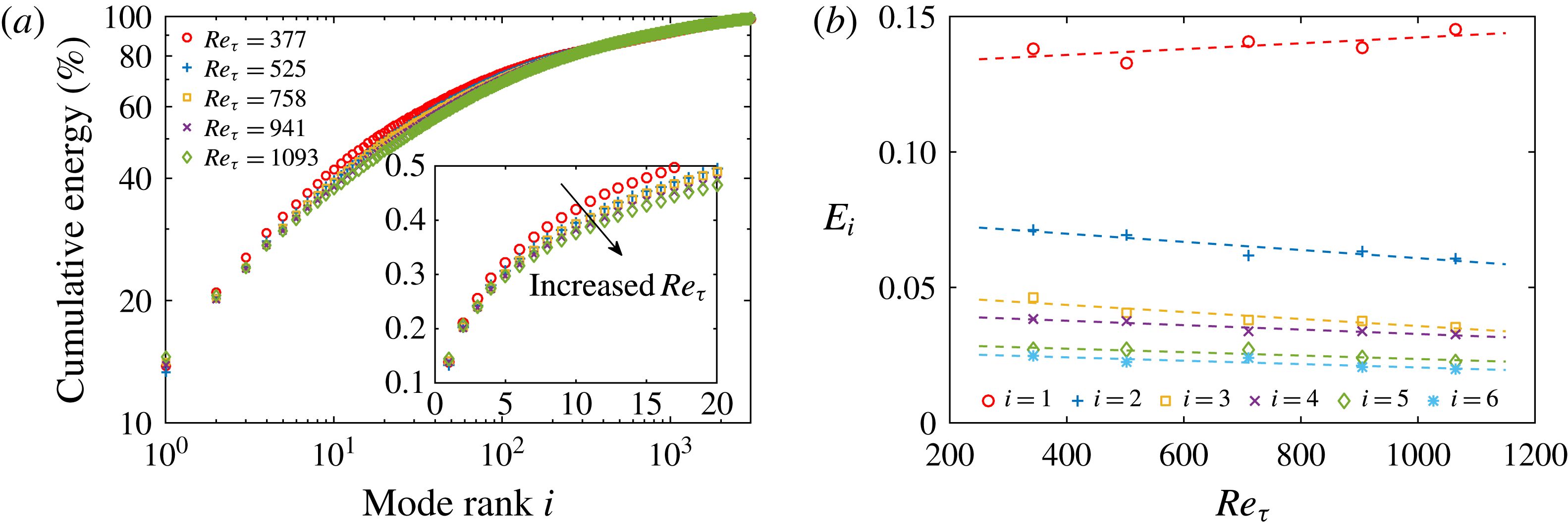
the corresponding eigenvalue, are shown in figure 2(a). It indicates an increasing TKE contribution from higher-order modes at higher
 $Re_{\unicode[STIX]{x1D70F}}$
, consistent with figure 2(b), which shows that
 $E_{i}$
of the leading-order
 $i$
th modes (with
 $i=2{-}5$
) decreases with the increase in
 $Re_{\unicode[STIX]{x1D70F}}$
.
Wu & Christensen (Reference Wu and Christensen2010) set
 $50\,\%$
TKE recovery, i.e.
 $\sum _{n=1}^{i}E_{n}=0.5$
, as the threshold to separate large- and small-scale components, based on which a group of the first six modes in the smooth-wall case at
 $Re_{\unicode[STIX]{x1D703}}=8200$
(or
 $Re_{\unicode[STIX]{x1D70F}}=3470$
) was selected to form a low-pass filter. In the present case of
 $Re_{\unicode[STIX]{x1D70F}}=377$
, the first 18 modes capture approximately
 $50\,\%$
of the resolved TKE, but this number increases to 26 in the
 $Re_{\unicode[STIX]{x1D70F}}=1093$
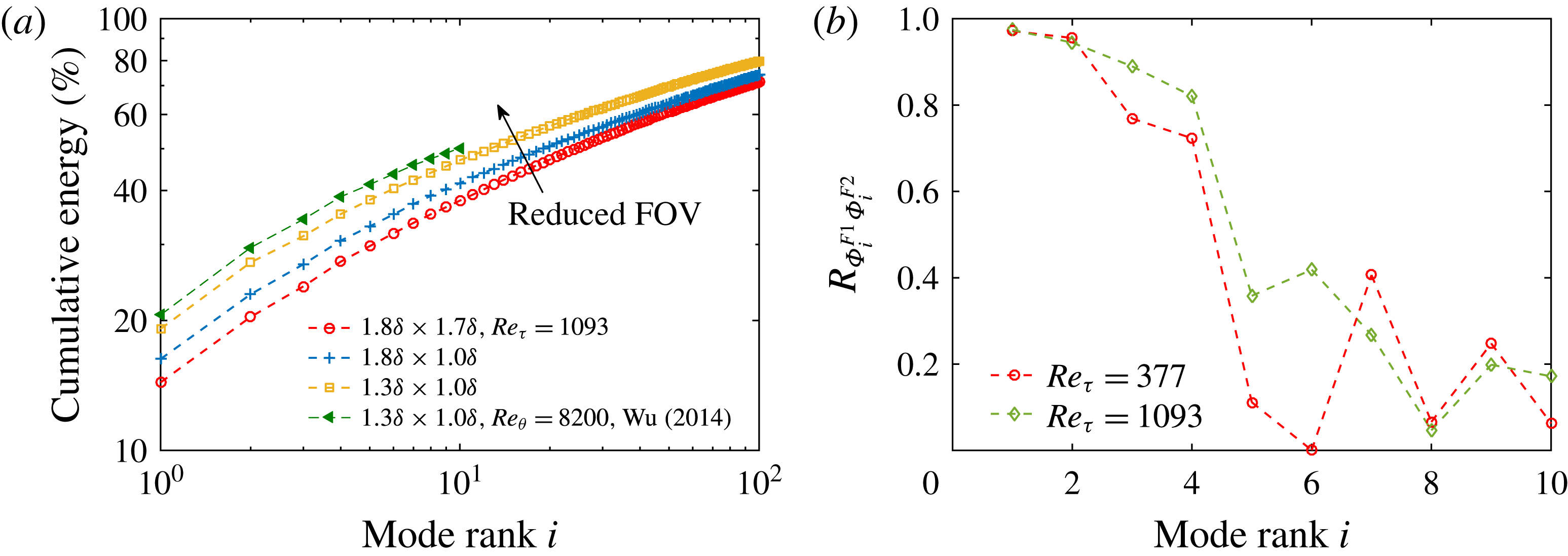
case; all are remarkably larger than that in Wu & Christensen (Reference Wu and Christensen2010). In our view, such a discrepancy is attributed to the larger spatial domain being analysed here. Figure 3(a) shows that by deliberately truncating the FOV, leading-order modes gradually made larger TKE contributions. A distribution of
 $E_{i}(i)$
close to that of Wu (Reference Wu2014) can be obtained at the same FOV (
 $1.3\unicode[STIX]{x1D6FF}\times 1.0\unicode[STIX]{x1D6FF}$
), despite the notable difference in
 $Re_{\unicode[STIX]{x1D70F}}$
. Interestingly, the eigenmodes of the first four leading-order modes are less sensitive to the variations in the FOV. This can be evidenced by figure 3(b), which shows that, in the presently studied
 $Re_{\unicode[STIX]{x1D70F}}$
range, the correlation between
 $\unicode[STIX]{x1D6F7}_{i}$
with a FOV of
 $1.8\unicode[STIX]{x1D6FF}\times 1.7\unicode[STIX]{x1D6FF}$
and that with a FOV of
 $1.3\unicode[STIX]{x1D6FF}\times 1.0\unicode[STIX]{x1D6FF}$
is rather high when
 $i\leqslant 4$
. In the following, an alternative criterion for selecting a group of leading-order modes as the low-pass filter will be constructed through spatio-temporal coherence analysis.
(a) Cumulative TKE contribution of the POD modes: ○,
 $Re_{\unicode[STIX]{x1D70F}}=377$
;
 $+$
,
 $Re_{\unicode[STIX]{x1D70F}}=525$
; ▫,
 $Re_{\unicode[STIX]{x1D70F}}=758$
;
 $\times$
,
 $Re_{\unicode[STIX]{x1D70F}}=941$
; and ♢,
 $Re_{\unicode[STIX]{x1D70F}}=1093$
. (b) Relative TKE portion of the leading-order
 $i$
th mode: ○,
 $i=1$
;
 $+$
,
 $i=2$
; ▫,
 $i=3$
;
 $\times$
,
 $i=4$
; ♢,
 $i=5$
; and *,
 $i=6$
.

Effect of FOV on (a) the cumulative TKE contribution and (b) the eigenmode of the leading-order
 $i$
th mode. In (a), the snapshot ensemble of the
 $Re_{\unicode[STIX]{x1D70F}}=1093$
case is truncated to different FOV: ○,
 $1.8\unicode[STIX]{x1D6FF}\times 1.7\unicode[STIX]{x1D6FF}$
;
 $+$
,
 $1.8\unicode[STIX]{x1D6FF}\times 1.0\unicode[STIX]{x1D6FF}$
; and ▫,
 $1.3\unicode[STIX]{x1D6FF}\times 1.0\unicode[STIX]{x1D6FF}$
; ◃, the data of Wu (Reference Wu2014) with
 $Re_{\unicode[STIX]{x1D703}}=8200$
and FOV of
 $1.3\unicode[STIX]{x1D6FF}\times 1.0\unicode[STIX]{x1D6FF}$
. In (b),
 $R_{\unicode[STIX]{x1D6F7}_{i}^{F1}\unicode[STIX]{x1D6F7}_{i}^{F2}}$
is the correlation coefficient between the
 $i$
th eigenmode
 $\unicode[STIX]{x1D6F7}_{i}$
with different FOV; the superscripts
 $(\cdot )^{F1}$
and
 $(\cdot )^{F2}$
indicate a FOV of
 $1.8\unicode[STIX]{x1D6FF}\times 1.7\unicode[STIX]{x1D6FF}$
and
 $1.2\unicode[STIX]{x1D6FF}\times 1.0\unicode[STIX]{x1D6FF}$
, respectively.

3.1 Eigenmodes of the leading-order POD modes
The eigenmodes
 $\unicode[STIX]{x1D6F7}_{i}(x,y)$
of the first six POD modes in the
 $Re_{\unicode[STIX]{x1D70F}}=377$
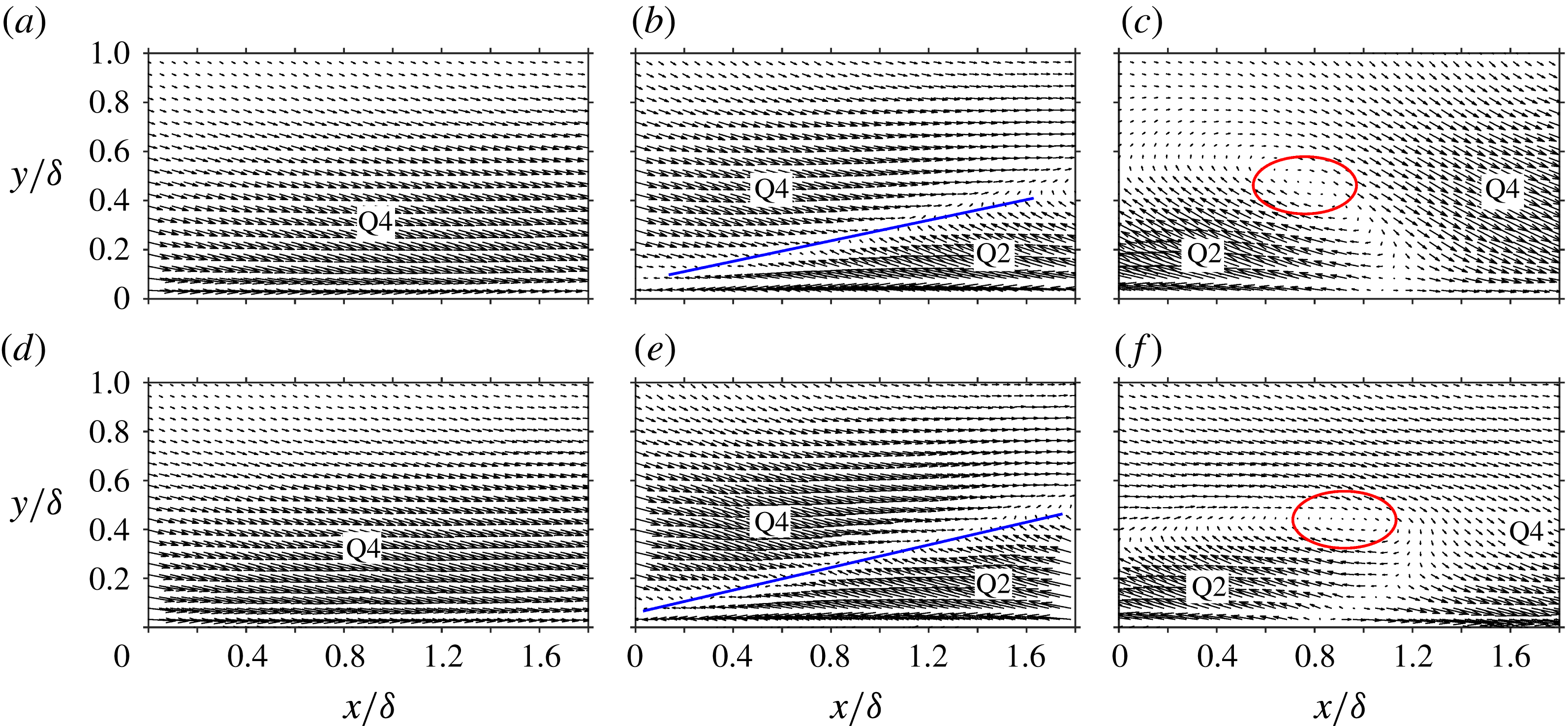
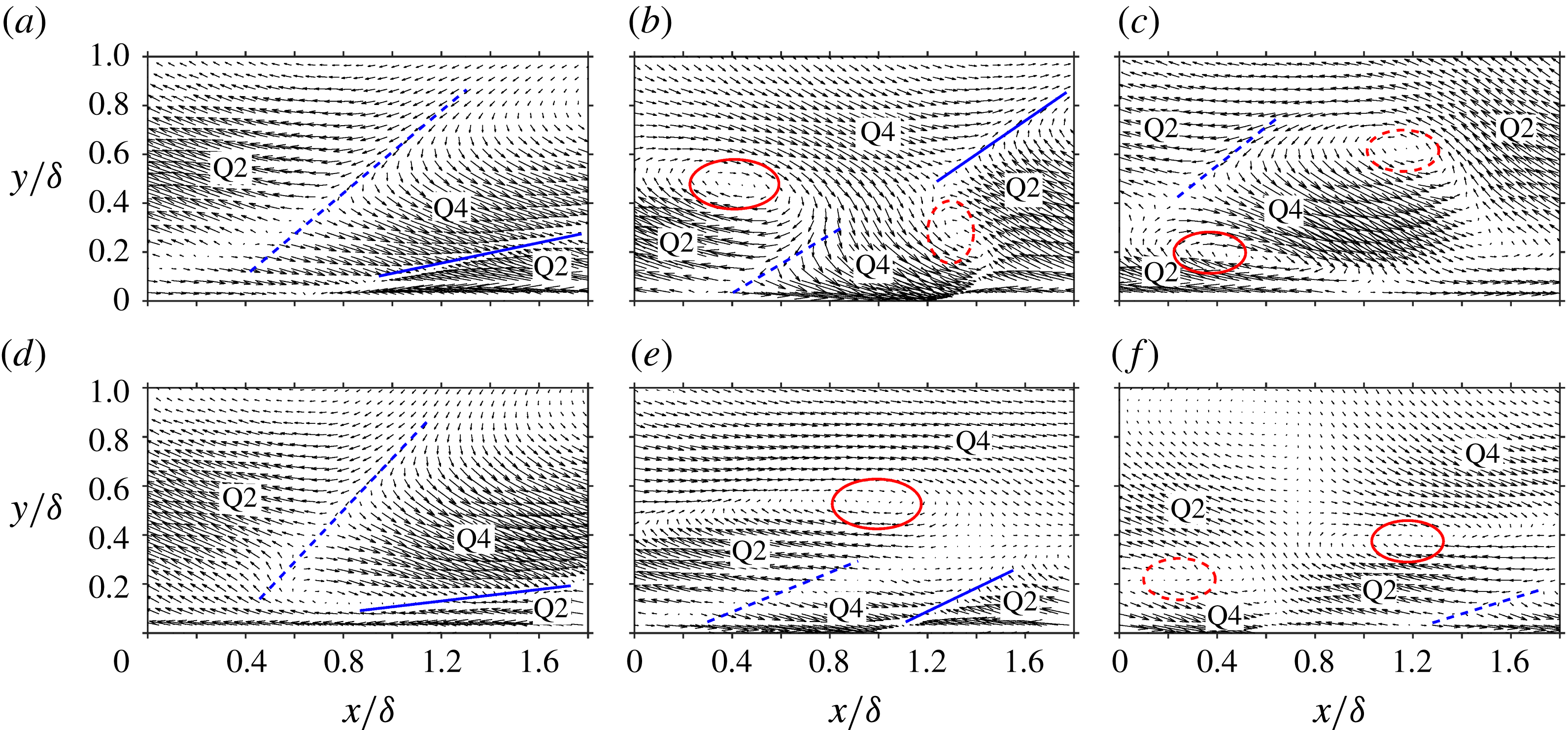
and 1093 cases are compared in figures 4 and 5. Topological similarity of
 $\unicode[STIX]{x1D6F7}_{i}$
can be observed in the first four modes. Such a similarity is also found in other cases, implying a topological invariant of the first four modes, at least in the presently studied
 $Re_{\unicode[STIX]{x1D70F}}$
range.
Quadrant analysis (Lu & Willmarth Reference Lu and Willmarth1973) is then conducted to categorize the characteristic topology of the leading-order modes. As indicated in figure 4,
 $\unicode[STIX]{x1D6F7}_{1}$
of the first mode presents one large-scale Q4 event (
 $\unicode[STIX]{x1D6F7}^{u}>0$
and
 $\unicode[STIX]{x1D6F7}^{v}<0$
, with the superscripts
 $(\cdot )^{u}$
and
 $(\cdot )^{v}$
indicating the streamwise and wall-normal components, respectively) spanning the whole boundary layer thickness. One pair of Q2 (
 $\unicode[STIX]{x1D6F7}^{u}<0$
and
 $\unicode[STIX]{x1D6F7}^{v}>0$
) and Q4 events appears in
 $\unicode[STIX]{x1D6F7}_{2}$
of the second mode. They converge to each other, with an interface being formed in the middle (indicated by solid lines in figure 4
b,e). The inclination angle of this interface is approximately
 $14^{\circ }$
, consistent with the values of the inclined imprints of the hairpin packets (Adrian et al.
Reference Adrian, Meinhart and Tomkins2000; Christensen & Adrian Reference Christensen and Adrian2001; Wu Reference Wu2014).
For the third mode,
 $\unicode[STIX]{x1D6F7}_{3}$
is characterized as a clockwise-rotating motion with a length scale that is considerably larger than those of typical prograde vortices (Natrajan, Wu & Christensen Reference Natrajan, Wu and Christensen2007; Herpin et al.
Reference Herpin, Stanislas, Foucaut and Coudert2013). Such a swirling pattern is partly visualized in
 $\unicode[STIX]{x1D6F7}_{2}$
(downstream of the Q2/Q4 interface at about
 $x/\unicode[STIX]{x1D6FF}=1.7$
,
 $y/\unicode[STIX]{x1D6FF}=0.4$
in figure 4
b,e), and seems to be formed by the Q1 and Q3 events that separate the upstream Q2 and downstream Q4 events in
 $\unicode[STIX]{x1D6F7}_{3}$
. Note that the flow pattern in the upstream (at about
 $x/\unicode[STIX]{x1D6FF}=0.4$
,
 $y/\unicode[STIX]{x1D6FF}=0.4$
in figure 4
c and 4
f) also resembles the Q2/Q4 interface in
 $\unicode[STIX]{x1D6F7}_{2}$
. Therefore, it is conjectured that
 $\unicode[STIX]{x1D6F7}_{2}$
and
 $\unicode[STIX]{x1D6F7}_{3}$
only differ from each other by a phase shift and jointly depict the signature of a large-scale structure convecting downstream. Owing to the limited FOV, a complete picture of this structure is not available yet; however, it deserves to be studied in a wider spatial domain in the future. Moreover, it is stressed that there is a slight difference in the topological pattern of
 $\unicode[STIX]{x1D6F7}_{3}$
between figure 4(c,f), suggesting the existence of a mild
 $Re$
effect.
Vector plot of the eigenmode
 $\unicode[STIX]{x1D6F7}_{i}(x,y)$
of the leading-order
 $i$
th POD mode with (a–c)
 $Re_{\unicode[STIX]{x1D70F}}=377$
and (d–f)
 $Re_{\unicode[STIX]{x1D70F}}=1093$
: (a,d)
 $i=1$
; (b,e)
 $i=2$
; and (c,f)
 $i=3$
.

Vector plot of the eigenmode
 $\unicode[STIX]{x1D6F7}_{i}(x,y)$
of the leading-order
 $i$
th POD mode with (a–c)
 $Re_{\unicode[STIX]{x1D70F}}=377$
and (d–f)
 $Re_{\unicode[STIX]{x1D70F}}=1093$
: (a,d)
 $i=4$
; (b,e)
 $i=5$
; and (c,f)
 $i=6$
.

In the fourth mode, the converging Q2/Q4 event remains visible in the downstream part of
 $\unicode[STIX]{x1D6F7}_{4}$
(after
 $x/\unicode[STIX]{x1D6FF}=1$
in figure 5
a,d). An additional Q2 event appears upstream of and above the Q4 event, forming another diverging Q4/Q2 pair. The interface clapped in the middle (indicated by dashed lines in figure 5
a,d) has an inclination angle of approximately
 $45^{\circ }$
. Such a diverging Q4/Q2 pattern resembles the conditional-averaged velocity field associated with a strong backscatter event as revealed by Natrajan & Christensen (Reference Natrajan and Christensen2006), who regarded it as the boundary between two successive hairpin packets.
For higher-order POD modes, the eigenmodes become hierarchically complicated, together with a distinct
 $Re$
dependence; see figure 5 for example. It is impracticable to describe them by a simple combination of several large-scale quadrant events.
3.2 Coupling of the leading-order POD modes
To explore the dynamic correlation between the leading-order modes, their time coefficients
 $a_{i}$
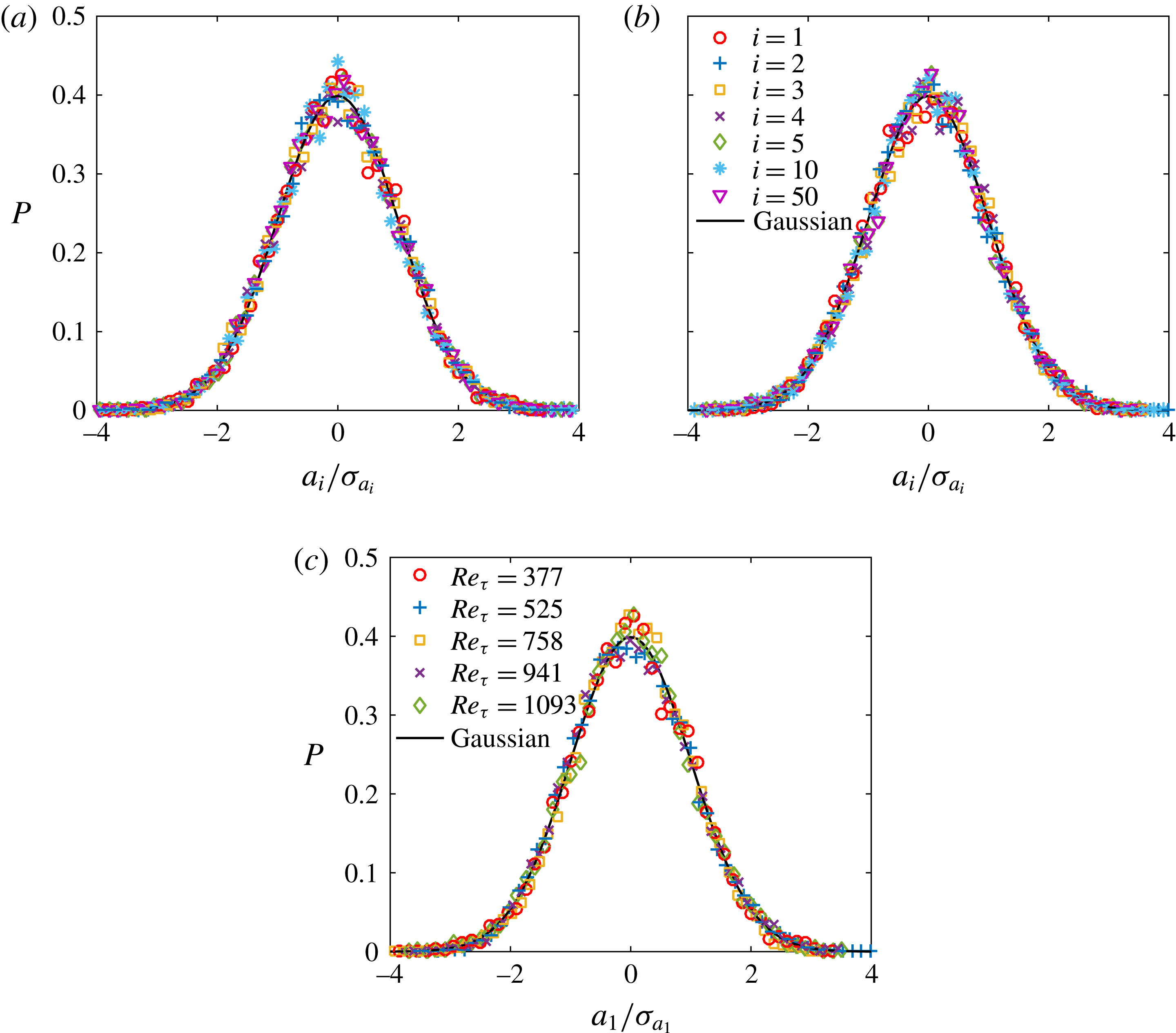
are further analysed. Figure 6 shows that, for the
 $i$
th mode until
 $i=50$
, the probability density function (p.d.f.) of the normalized
 $a_{i}/\unicode[STIX]{x1D70E}_{a_{i}}$
(with
 $\unicode[STIX]{x1D70E}_{a_{i}}$
being the root-mean-square (r.m.s.) value of
 $a_{i}$
) always follows a normal distribution that is independent of
 $Re$
. This seems to suggest that the spatial coherence embodied by each mode appears in time randomly.
P.d.f. of the time coefficient
 $a_{i}$
of the
 $i$
th POD mode. In (a) and (b),
 $Re_{\unicode[STIX]{x1D70F}}=377$
and 1093, respectively: ○,
 $i=1$
;
 $+$
,
 $i=2$
; ▫,
 $i=3$
;
 $\times$
,
 $i=4$
; ♢,
 $i=5$
; *,
 $i=10$
; ▿,
 $i=50$
. In (c),
 $i=1$
: ○,
 $Re_{\unicode[STIX]{x1D70F}}=377$
;
 $+$
,
 $Re_{\unicode[STIX]{x1D70F}}=525$
; ▫,
 $Re_{\unicode[STIX]{x1D70F}}=758$
;
 $\times$
,
 $Re_{\unicode[STIX]{x1D70F}}=941$
; ♢,
 $Re_{\unicode[STIX]{x1D70F}}=1093$
. Solid lines represent the normal distribution; and
 $a_{i}$
is normalized by its r.m.s. value
 $\unicode[STIX]{x1D70E}_{a_{i}}$
.

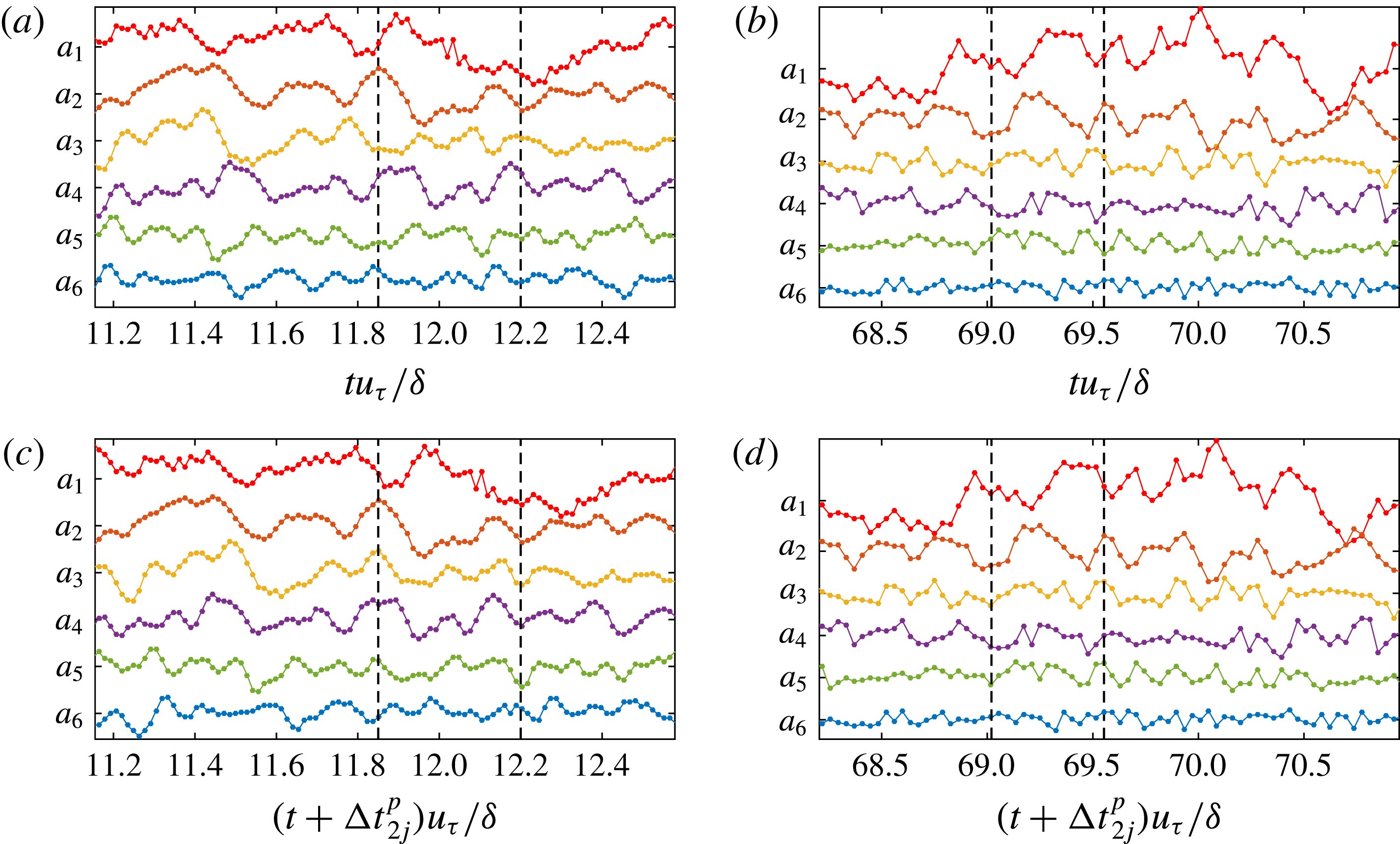
Time series of the time coefficients of the first six POD modes normalized by
 $\unicode[STIX]{x1D6FF}/u_{\unicode[STIX]{x1D70F}}$
: (a,c)
 $a_{j}(t)$
; (b,d)
 $a_{j}(t+\unicode[STIX]{x0394}t_{2j}^{\,p})$
, where
 $\unicode[STIX]{x0394}t_{2j}^{\,p}$
is the ‘optimal’ time lag between
 $a_{j}$
and
 $a_{2}$
; (a,b)
 $Re_{\unicode[STIX]{x1D70F}}=377$
; (c,d)
 $Re_{\unicode[STIX]{x1D70F}}=1093$
. Dashed vertical lines indicate the phase alignment in (b) and (d).

Wu (Reference Wu2014) identified the so-called ‘dominant turbulent structures’ from instantaneous snapshots presenting extremely large values of
 $a_{i}$
(with
 $i=1$
or 2). These structures were regarded as the major contributors to the first two POD modes and were believed to be consistent with the hairpin-packet imprints. To keep the topological similarity between
 $\unicode[STIX]{x1D6F7}_{1,2}$
and one snapshot with large
 $a_{1,2}$
,
 $a_{i}$
of the rest modes of this snapshot should either be close to zero or jointly cancel each other. Referring to the time series
 $a_{i}(t)$
of the first six modes in the
 $Re_{\unicode[STIX]{x1D70F}}=377$
and 1093 cases, as shown in figure 7(a,c), this condition is seldom satisfied. In our view, there might be another scenario, i.e. the leading-order modes dynamically acting as a whole, contributing to the large-scale imprints of the hairpin packets.
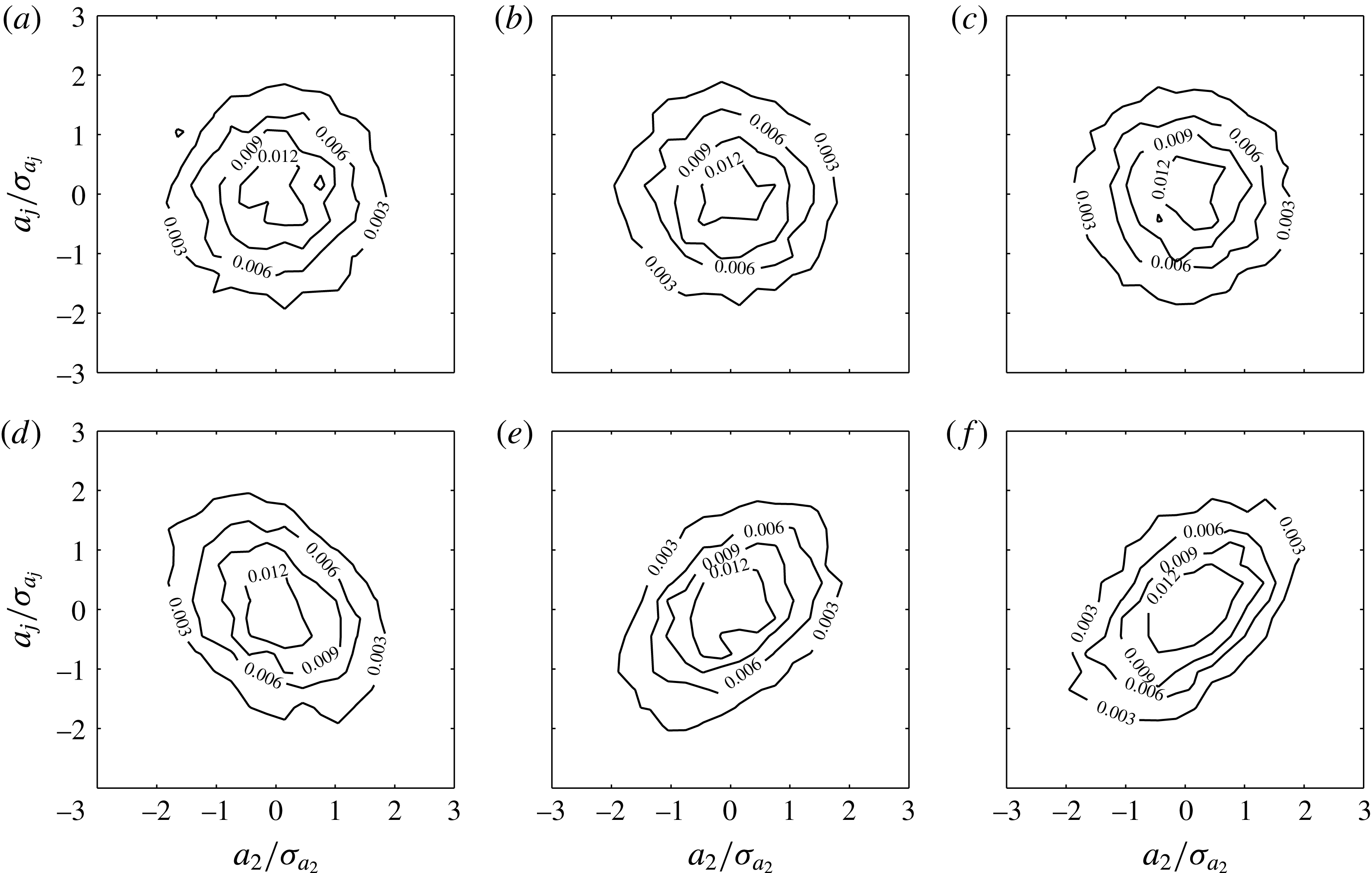
The joint p.d.f.
 $P(a_{i}/\unicode[STIX]{x1D70E}_{a_{i}},a_{j}/\unicode[STIX]{x1D70E}_{a_{j}})$
is then inspected. In all the
 $Re$
cases, any two normalized
 $a_{i}$
and
 $a_{j}$
(with
 $i,j\leqslant 50$
) follow bivariate normal distributions without any discernible phase preference (see figure 8
a–c for an illustration). Nevertheless, a careful examination of figure 7(a,c) suggests that
 $a_{i}(t)$
of the leading-order modes do present phase-shift coherence with each other. Following Hellström et al. (Reference Hellström, Ganapathisubramani and Smits2015), the time-lag correlation between
 $a_{i}$
and
 $a_{j}$
is calculated to quantify such coherence:
 $$\begin{eqnarray}R_{ij}(\unicode[STIX]{x0394}t)=\frac{\overline{a_{i}(t)a_{j}(t+\unicode[STIX]{x0394}t)}}{\unicode[STIX]{x1D70E}_{a_{i}}\unicode[STIX]{x1D70E}_{a_{j}}}.\end{eqnarray}$$
In (3.2),
 $\overline{(\cdot )}$
is the average over time,
 $\unicode[STIX]{x1D70E}_{a_{i,j}}$
is the standard deviation of
 $a_{i,j}$
, and
 $\unicode[STIX]{x0394}t$
is the time lag. Note that figure 7 shows that the present sampling frequency (
 $f_{s}=7.5~\text{Hz}$
) is sufficient for the time-lag correlation analysis of the leading-order modes even at the highest
 $Re$
.
Joint p.d.f. between
 $a_{2}(t)$
and
 $a_{j}(t)$
in (a–c) and between
 $a_{2}(t)$
and
 $a_{j}(t+\unicode[STIX]{x0394}t_{2j}^{\,p})$
in (d–f), for
 $Re_{\unicode[STIX]{x1D70F}}=377$
: (a,d)
 $j=1$
; (b,e)
 $j=3$
; and (c,f)
 $j=4$
. The contour level ranges from
 $0.3\,\%$
to
 $1.2\,\%$
with a step of
 $0.3\,\%$
. Here
 $a_{2}$
and
 $a_{j}$
are normalized by their r.m.s. values
 $\unicode[STIX]{x1D70E}_{a_{2}}$
and
 $\unicode[STIX]{x1D70E}_{a_{j}}$
, respectively.

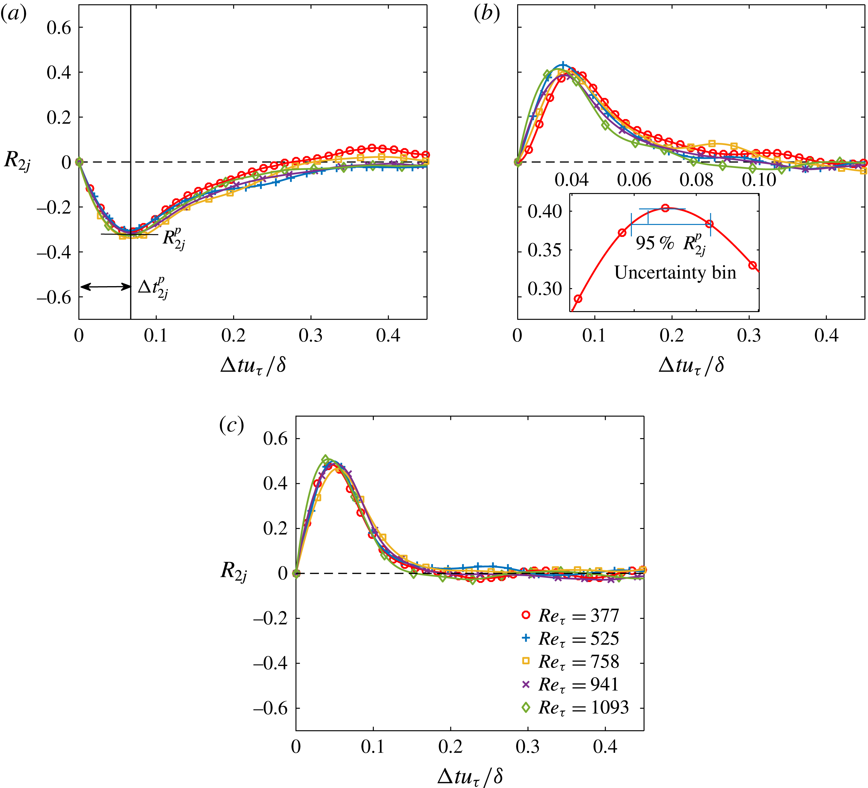
The time-lag correlation coefficient
 $R_{2j}$
between
 $a_{2}(t)$
and
 $a_{j}(t+\unicode[STIX]{x0394}t)$
, for (a)
 $j=1$
, (b)
 $j=3$
and (c)
 $j=4$
: ○,
 $Re_{\unicode[STIX]{x1D70F}}=377$
;
 $+$
,
 $Re_{\unicode[STIX]{x1D70F}}=525$
; ▫,
 $Re_{\unicode[STIX]{x1D70F}}=758$
;
 $\times$
,
 $Re_{\unicode[STIX]{x1D70F}}=941$
; ♢,
 $Re_{\unicode[STIX]{x1D70F}}=1093$
. Here
 $\unicode[STIX]{x0394}t$
is normalized by
 $\unicode[STIX]{x1D6FF}/u_{\unicode[STIX]{x1D70F}}$
. The inset in (b) illustrates the definition of the uncertainty of both the correlation peak
 $|R_{2j}^{p}|$
and the corresponding ‘optimal’ time lag
 $\unicode[STIX]{x0394}t_{2i}^{p}$
. The red solid curve is a localized Gaussian fit around (
 $|R_{2j}^{p}|,\unicode[STIX]{x0394}t_{2i}^{p}$
).

Figure 9 plots
 $R_{2j}$
between
 $a_{2}$
and
 $a_{j}$
(with
 $j=1$
, 3 and 4) as a function of
 $\unicode[STIX]{x0394}t$
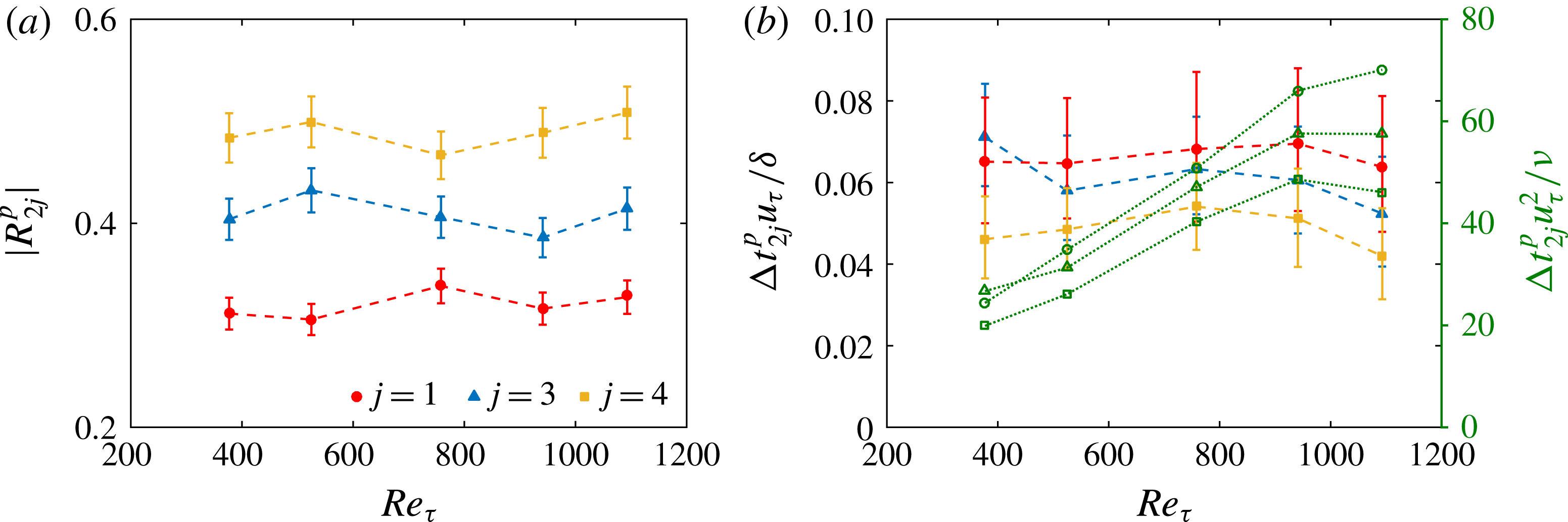
. In all the studied cases, a correlation peak
 $|R_{2j}^{p}|$
with a rather high magnitude (
 $|R_{2j}^{p}|>0.3$
, as shown in figure 10
a) can always be detected at an ‘optimal’ time lag
 $\unicode[STIX]{x0394}t_{2j}^{\,p}$
. As illustrated in the inset of figure 9(b), the uncertainty of
 $|R_{2j}^{p}|$
is estimated by a local Gaussian fit around the peak, while that of
 $\unicode[STIX]{x0394}t_{2j}^{\,p}$
is defined as the bin spanning the 95 % range of
 $R_{2j}^{p}$
; all uncertainties are summarized in figure 10 as error bars. Figure 7(b,d) and figure 8(d–f) show that the shifted
 $a_{j}(t+\unicode[STIX]{x0394}t_{2j}^{\,p})$
now present remarkable phase alignment with
 $a_{2}(t)$
. More interestingly, all the
 $R_{2j}\sim \unicode[STIX]{x0394}t$
curves in figure 9 with various
 $Re$
collapse with each other when normalizing
 $\unicode[STIX]{x0394}t$
by the eddy turnover time
 $\unicode[STIX]{x1D6FF}/u_{\unicode[STIX]{x1D70F}}$
. The corresponding
 $\unicode[STIX]{x0394}t_{2j}^{\,p}u_{\unicode[STIX]{x1D70F}}/\unicode[STIX]{x1D6FF}$
(shown in figure 10
b) presents a weak
 $Re$
dependence when taking the estimation uncertainty into account, in distinct contrast to that in an inner scaling by
 $\unicode[STIX]{x1D708}/u_{\unicode[STIX]{x1D70F}}^{2}$
. This implies the large-scale nature of the temporal characteristics of the first four leading-order modes.
(a) The
 $Re$
dependence of the correlation peak
 $|R_{2j}^{p}|$
and (b) the ‘optimal’ time lag
 $\unicode[STIX]{x0394}t_{2j}^{\,p}$
: ●,
 $j=1$
; ▴,
 $j=3$
; ▪,
 $j=4$
. In (b),
 $\unicode[STIX]{x0394}t_{2j}^{\,p}$
is normalized by either
 $\unicode[STIX]{x1D6FF}/u_{\unicode[STIX]{x1D70F}}$
(solid symbols with vertical axis on a) or
 $\unicode[STIX]{x1D708}/u_{\unicode[STIX]{x1D70F}}^{2}$
(hollow symbols with vertical axis on b). The error bars show the uncertainty of both
 $|R_{2j}^{p}|$
and
 $\unicode[STIX]{x0394}t_{2j}^{\,p}$
estimated by the method illustrated in figure 9
b.

Matrix plot of the correlation peak
 $\left|R_{ij}^{p}\right|$
between
 $a_{i}(t)$
and
 $a_{j}(t+\unicode[STIX]{x0394}t_{2j}^{\,p})$
: (a)
 $Re_{\unicode[STIX]{x1D70F}}=377$
; (b)
 $Re_{\unicode[STIX]{x1D70F}}=525$
; (c)
 $Re_{\unicode[STIX]{x1D70F}}=758$
; (d)
 $Re_{\unicode[STIX]{x1D70F}}=941$
; (e)
 $Re_{\unicode[STIX]{x1D70F}}=1093$
. Only the cell with
 $|R_{ij}^{p}|>0.3$
is visualized.

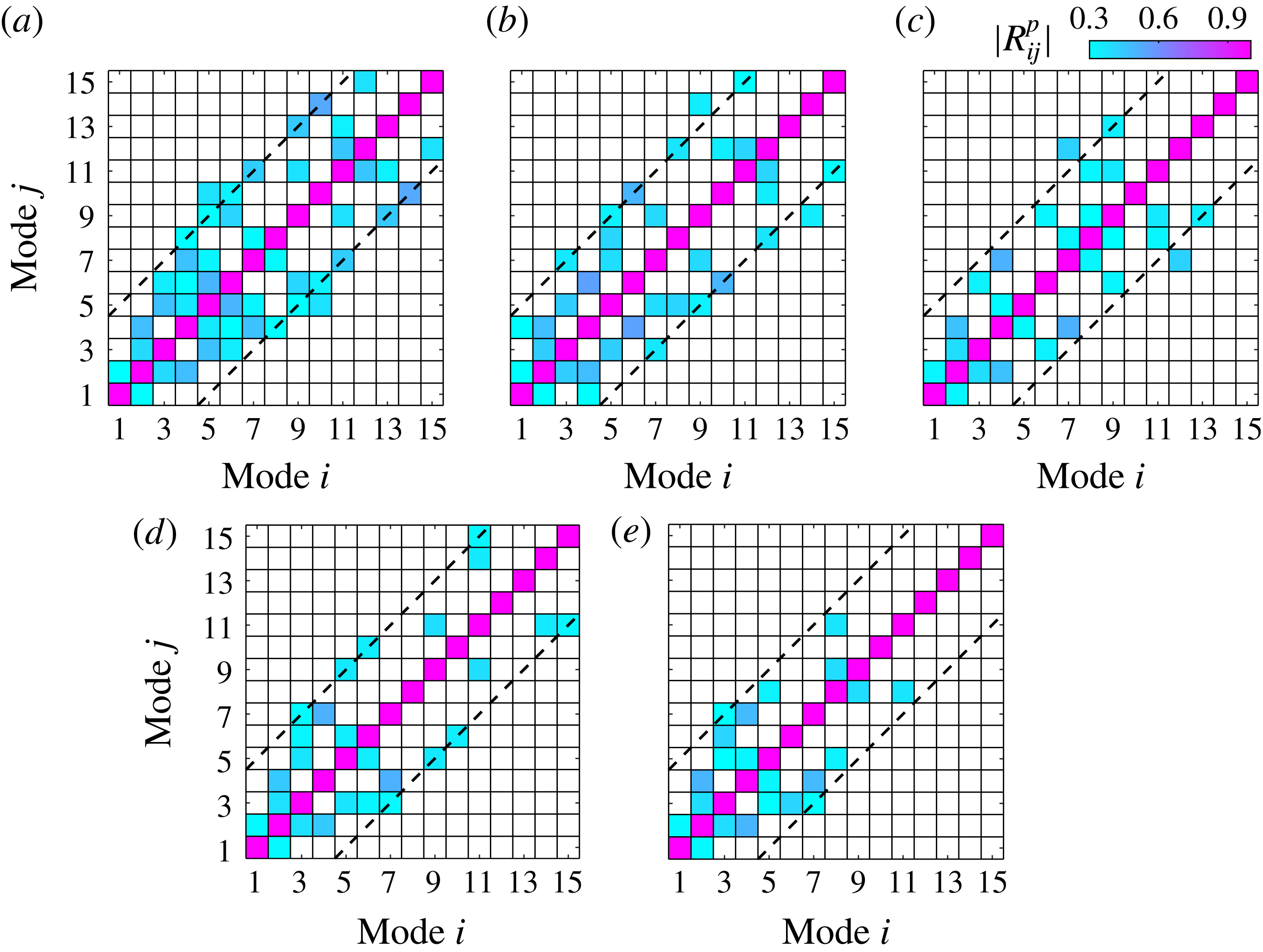
For a systematic depiction,
 $|R_{ij}^{p}|$
of the first 15 modes are presented in a matrix form in figure 11, in which a cutoff threshold of
 $|R_{ij}^{p}|=0.3$
is applied to mask those
 $(a_{i},a_{j})$
pairs being less correlated. In general, strong correlations only exist between two modes whose rank gaps
 $\left|i-j\right|$
are smaller than 5 (as indicated by the dashed lines in figure 11). Lower
 $Re$
results in a higher rank of the modes that remain correlated with their neighbours. This might be attributed to the insufficient scale separation in the low-
 $Re$
case. As
 $Re_{\unicode[STIX]{x1D70F}}$
increases beyond 1000, the number of correlated modes quickly decreases. Nevertheless,
 $a_{i}$
of the first four modes are persistently correlated with each other throughout the presently studied
 $Re$
range.
Rempfer & Fasel (Reference Rempfer and Fasel1994) showed that, in a transitional boundary layer, two neighbouring leading-order POD modes with equivalent eigenvalues can be grouped into one conjugated pair to depict the convective motion of the same structure. For a fully developed turbulent boundary layer with abundant structures and complicated inter-scale interactions, finding pairs of conjugated modes is impracticable. In fact, Hellström et al. (Reference Hellström, Ganapathisubramani and Smits2015) identified the existence of low-energy intermediate modes responsible for the transition between energy-containing large-scale modes. The present temporal correlation analysis suggests that, despite the energy hierarchy, the first four modes, which present strong spatial similarity, also exhibit dynamical coherence with each other. They can thus be grouped as a whole to jointly characterize the spatio-temporal evolution of the same type of large-scale structures.
4 Statistical picture of the hairpin-packet imprints
Using the group of the first four POD modes, a low-order representation of the fluctuating velocity fields
 $\boldsymbol{V}^{L}$
can be obtained via
 $\boldsymbol{V}(\boldsymbol{X},t)^{L}=\sum _{i=1}^{4}a_{i}(t)\unicode[STIX]{x1D6F7}_{i}(\boldsymbol{X})$
. In the following, the superscript
 $(\cdot )^{L}$
denotes the low-order reconstruction.
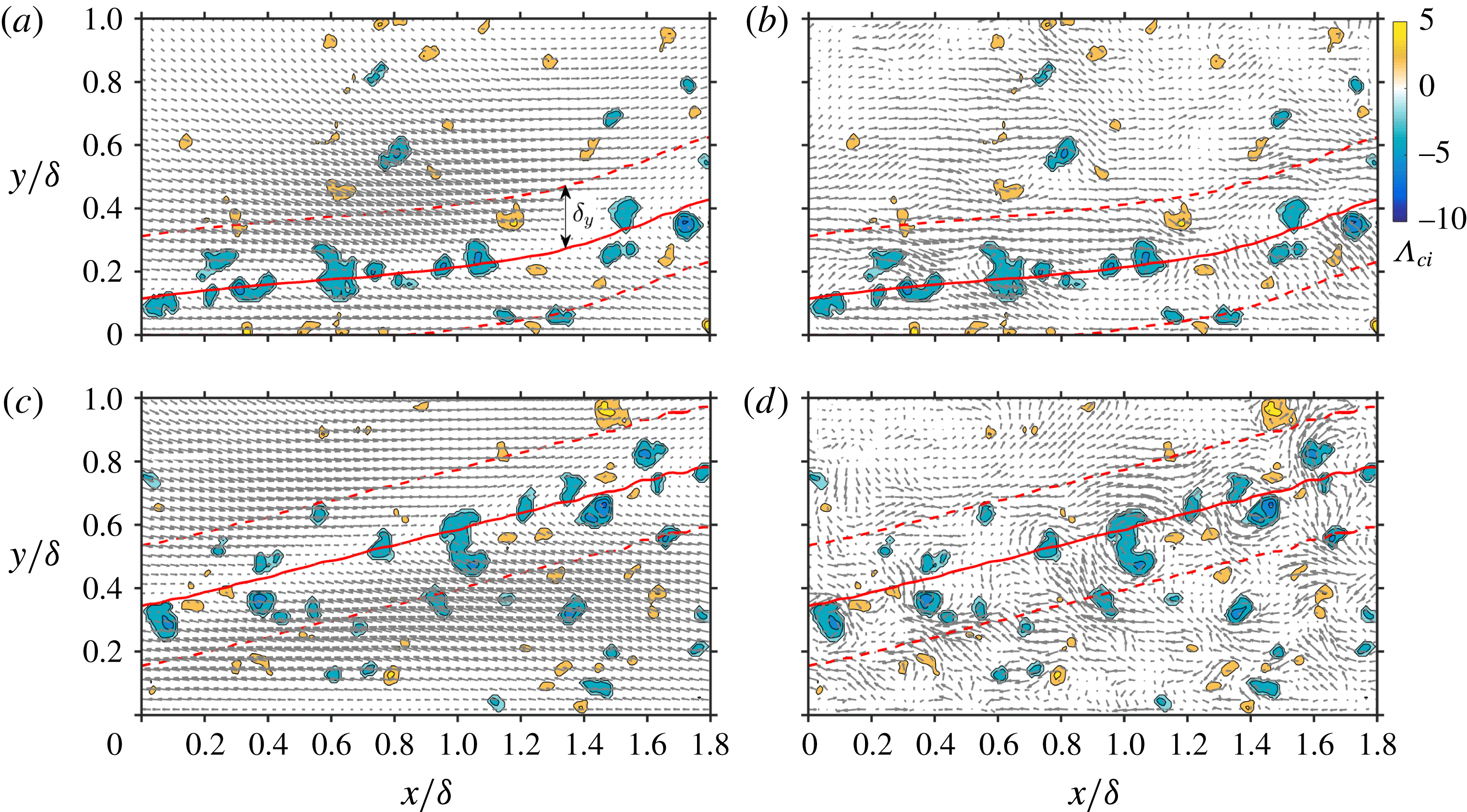
Figure 12(a,c) illustrates a typical snapshot of
 $\boldsymbol{V}^{L}$
at
 $Re_{\unicode[STIX]{x1D70F}}=304$
and 1093, respectively. The swirling strength
 $\unicode[STIX]{x1D6EC}_{ci}$
calculated from the full-order
 $\boldsymbol{V}$
is also shown to depict the spanwise rotated vortices. Note that
 $\unicode[STIX]{x1D6EC}_{ci}=\unicode[STIX]{x1D706}_{ci}\unicode[STIX]{x1D714}_{z}/\left|\unicode[STIX]{x1D714}_{z}\right|$
, with
 $\unicode[STIX]{x1D706}_{ci}$
being the imaginary part of the complex eigenvalue of the local velocity gradient tensor (Zhou et al.
Reference Zhou, Adrian, Balachandar and Kendall1999). Owing to the 2D PIV measurement, the velocity gradient tensor is tailored to a 2D form when calculating
 $\unicode[STIX]{x1D706}_{ci}$
(Adrian et al.
Reference Adrian, Meinhart and Tomkins2000; Wu & Christensen Reference Wu and Christensen2010). The sign of the local spanwise vorticity
 $\unicode[STIX]{x1D714}_{z}$
is assigned to
 $\unicode[STIX]{x1D6EC}_{ci}$
to indicate the sense of rotation. Chernyshenko et al. (Reference Chernyshenko, Di Cicca, Iollo, Smirnov, Sandham and Hu2006) recommended a proper filtering of the velocity field before calculating
 $\unicode[STIX]{x1D706}_{ci}$
to avoid artificial eddies associated with random noise. In this regard, the
 $\unicode[STIX]{x1D6EC}_{ci}$
fields are calculated from both the full-order
 $\boldsymbol{V}$
and the high-order
 $\boldsymbol{V}-\boldsymbol{V}^{L}$
. No remarkable difference is observed, suggesting the insignificant contribution of
 $\boldsymbol{V}^{L}$
to
 $\unicode[STIX]{x1D6EC}_{ci}$
.
As shown in figure 12(a,c), large-scale inclined interfaces separating the converging Q2/Q4 events are clearly visualized in the low-order
 $\boldsymbol{V}^{L}$
fields. In contrast, the full-order
 $\boldsymbol{V}$
fields (figure 12
b,d) fail to reveal such a pattern due to the distortion of small-scale vortices (indicated by
 $\unicode[STIX]{x1D6EC}_{ci}$
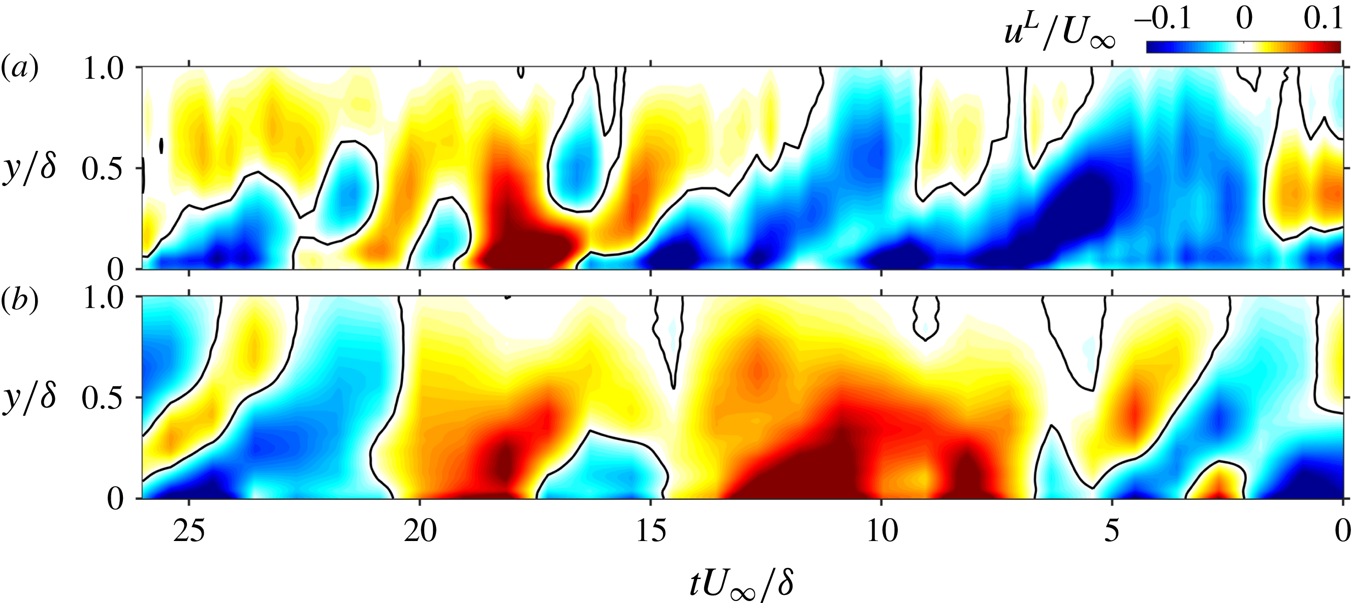
concentration regions in figure 12) discretely residing along the interfaces. Figure 13 invokes Taylor’s frozen hypothesis to show the
 $u^{L}$
component in a large streamwise domain at
 $Re_{\unicode[STIX]{x1D70F}}=304$
and 1093. The dominant structures below the interfaces are found to be the wall-attached LSMs of low-speed
 $u^{L}$
with a streamwise length up to several
 $\unicode[STIX]{x1D6FF}$
. Most LSMs extend into the outer region to form a spatial pattern consistent with the large-scale imprints of the hairpin packets (Adrian Reference Adrian2007). The streamwise alignment of several isolated LSMs, as has been observed in turbulent pipe flow by POD-based low-order characterization (Hellström & Smits Reference Hellström and Smits2014; Hellström et al.
Reference Hellström, Ganapathisubramani and Smits2015), is also observed here (see the region at
 $tU_{\infty }/\unicode[STIX]{x1D6FF}=5{-}15$
in figure 13
a for instance) to form a typical signature of VLSM.
Vector plot of the instantaneous snapshots of (a,c) the low-order
 $\boldsymbol{V}^{L}(x,y)$
and (b,d) the full-order
 $\boldsymbol{V}(x,y)$
: (a,b)
 $Re_{\unicode[STIX]{x1D70F}}=377$
; (c,d)
 $Re_{\unicode[STIX]{x1D70F}}=1093$
. The full-order
 $\unicode[STIX]{x1D6EC}_{ci}$
are shown as contours in cyan and yellow to indicate swirling motions with clockwise and anticlockwise rotations, respectively. The red bold solid lines and the red dashed lines represent the zero-
 $u^{L}$
lines and their
 $\pm 0.2\unicode[STIX]{x1D6FF}$
wall-normal offset. A supplementary animation corresponding to (a) is available online at https://doi.org/10.1017/jfm.2018.160 to depict the dynamical evolution of the large-scale interfaces revealed in
 $\boldsymbol{V}^{L}$
.

Distribution of the low-order
 $u^{L}$
in the (
 $tU_{\infty }/\unicode[STIX]{x1D6FF},y/\unicode[STIX]{x1D6FF}$
) plane in the middle of the streamwise FOV: (a)
 $Re_{\unicode[STIX]{x1D70F}}=377$
; (b)
 $Re_{\unicode[STIX]{x1D70F}}=1093$
. Bold solid lines indicate the region with
 $u^{L}=0$
.

4.1 Indicator of the interfaces of the hairpin packets
According to previous studies (Adrian Reference Adrian2007; Wu Reference Wu2014), the converging Q2/Q4 events and the associated large-scale interfaces in the low-order fields can be attributed to the interaction between the incoming flow and the collective backward induction of hierarchically aligned hairpin heads in a packet. In this scenario, a confluence line with zero speed will always be generated in the middle. The line of
 $u^{L}=0$
in the
 $\boldsymbol{V}^{L}$
field, in our view, will serve as a suitable indicator of the large-scale interfaces. Note that the diverging Q4/Q2 events will also produce zero-
 $u^{L}$
lines, which can be regarded as the dividing boundaries of two neighbouring hairpin packets (Natrajan & Christensen Reference Natrajan and Christensen2006). This case is excluded here by considering only zero-
 $u^{L}$
lines where the low-pass-filtered spanwise vorticities are negative, i.e.
 $\unicode[STIX]{x1D714}_{z}^{L}<0$
.
Typical zero-
 $u^{L}$
lines, which are obtained by connecting the zero-crossing points in the
 $u^{L}(y)$
profiles at each
 $x$
station, are illustrated in figures 12 and 13 as bold solid lines. In all the studied cases, more than 50 % of these zero-
 $u^{L}$
lines have a streamwise length
 $L_{x}$
longer than
 $\unicode[STIX]{x1D6FF}$
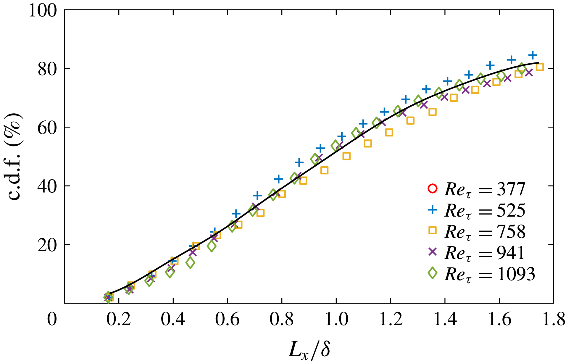
, as suggested by the cumulative distribution function (c.d.f.) of
 $L_{x}$
in figure 14. Owing to the truncation of the streamwise FOV, the right end of the
 $\text{c.d.f.}\sim L_{x}$
curves in figure 14 are underestimated; instead, one can obtain an impression on the possible extension of
 $L_{x}$
from figure 13. Visual inspection confirms that most zero-
 $u^{L}$
lines with positive inclination angles are in accordance with the inclined interfaces of the converging Q2/Q4 events. The justification is that no other typical eddies with equivalent length scales are likely to leave such large-scale imprints in the low-order fields.
The c.d.f. of the streamwise length
 $L_{x}$
of the zero-
 $u^{L}$
lines: ○,
 $Re_{\unicode[STIX]{x1D70F}}=377$
:
 $+$
,
 $Re_{\unicode[STIX]{x1D70F}}=525$
; ▫,
 $Re_{\unicode[STIX]{x1D70F}}=758$
;
 $\times$
,
 $Re_{\unicode[STIX]{x1D70F}}=941$
; and ♢,
 $Re_{\unicode[STIX]{x1D70F}}=1093$
.

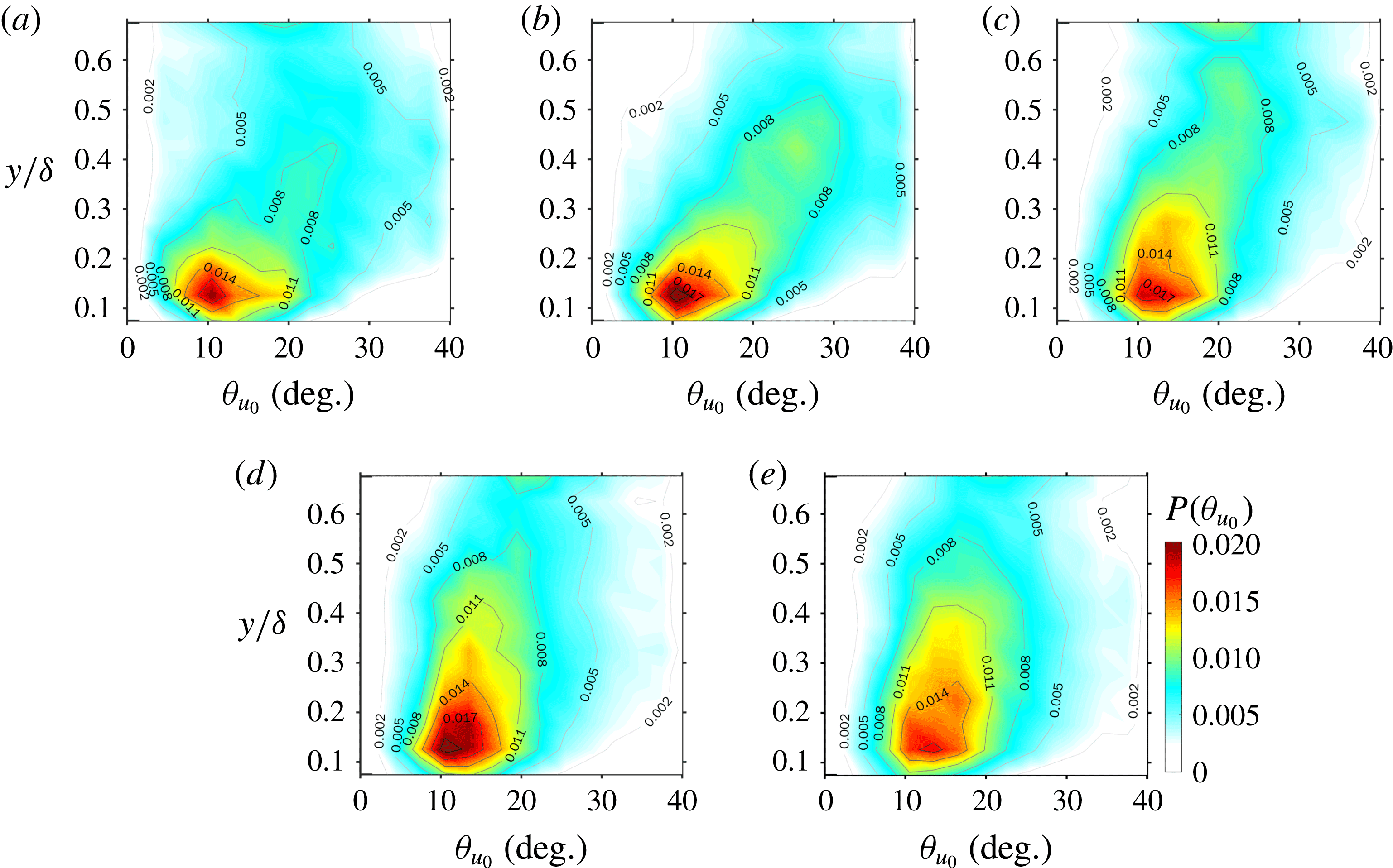
Figure 15 shows the wall-normal variation of the p.d.f. of the inclination angle
 $\unicode[STIX]{x1D703}_{u_{0}}$
of zero-
 $u^{L}$
lines, which are calculated by the local slope of the detected zero-
 $u^{L}$
lines at specified
 $y$
. Note that the negative
 $\unicode[STIX]{x1D703}_{u_{0}}$
events, whose occurrence probabilities are one-fifth lower than that of the positive
 $\unicode[STIX]{x1D703}_{u_{0}}$
events, are inconsistent with the inclined pattern of the interfaces and are not counted here. In each
 $Re$
case, a p.d.f. peak around
 $\unicode[STIX]{x1D703}_{u_{0}}=10^{\circ }{-}14^{\circ }$
is always presented at
 $y/\unicode[STIX]{x1D6FF}\approx 0.15$
, i.e. the upper bound of the log layer (Klewicki, Fife & Wei Reference Klewicki, Fife and Wei2009; Marusic et al.
Reference Marusic, Monty, Hultmark and Smits2013). Moreover,
 $P(\unicode[STIX]{x1D703}_{u_{0}})$
is right skewed in the log layer and below but gradually relaxes towards a symmetric distribution in the wake region and above. A smaller
 $Re$
results in a lower flow layer whereby such relaxation begins. The most probable value of
 $\unicode[STIX]{x1D703}_{u_{0}}$
monotonically increases with
 $y/\unicode[STIX]{x1D6FF}$
but decreases with
 $Re$
. In addition, the magnitude varies between
 $10^{\circ }$
and
 $25^{\circ }$
, falling in the range of the averaged inclination angle of the hairpin packets reported by previous studies (
 $15^{\circ }{-}20^{\circ }$
in Head & Bandyopadhyay (Reference Head and Bandyopadhyay1981);
 $12^{\circ }{-}20^{\circ }$
in Adrian et al. (Reference Adrian, Meinhart and Tomkins2000); and
 $20^{\circ }$
in Natrajan & Christensen (Reference Natrajan and Christensen2006)) via different detection methods. This provides evidence for the idea that the zero-
 $u^{L}$
lines capture the inclined geometric features of the hairpin packets.
Wall-normal variation of the p.d.f. of the inclination angle
 $\unicode[STIX]{x1D703}_{u_{0}}$
of the zero-
 $u^{L}$
lines: (a)
 $Re_{\unicode[STIX]{x1D70F}}=377$
; (b)
 $Re_{\unicode[STIX]{x1D70F}}=525$
; (c)
 $Re_{\unicode[STIX]{x1D70F}}=758$
; (d)
 $Re_{\unicode[STIX]{x1D70F}}=941$
; and (e)
 $Re_{\unicode[STIX]{x1D70F}}=1093$
.

4.2 Relationship between large-scale interface and uniform momentum zones
The definition of the zero-
 $u^{L}$
line implies a sharp jump of the full-order
 $u$
across it; this is somewhat similar to the feature of the so-called internal boundaries (IBs) of the uniform momentum zones (UMZs) (de Silva, Hutchins & Marusic Reference de Silva, Hutchins and Marusic2016). On considering that there are viewpoints that UMZs are kinematically linked to the signature of packet-like hairpin structures (Meinhart & Adrian Reference Meinhart and Adrian1995; Adrian et al.
Reference Adrian, Meinhart and Tomkins2000; de Silva et al.
Reference de Silva, Hutchins and Marusic2016), it is interesting to see whether the concept of zero-
 $u^{L}$
lines can be accommodated in the paradigm of UMZs.
The modal-velocity-based criterion proposed by Adrian et al. (Reference Adrian, Meinhart and Tomkins2000) and de Silva et al. (Reference de Silva, Hutchins and Marusic2016) is adopted here to detect UMZs from instantaneous
 $u(x,y)$
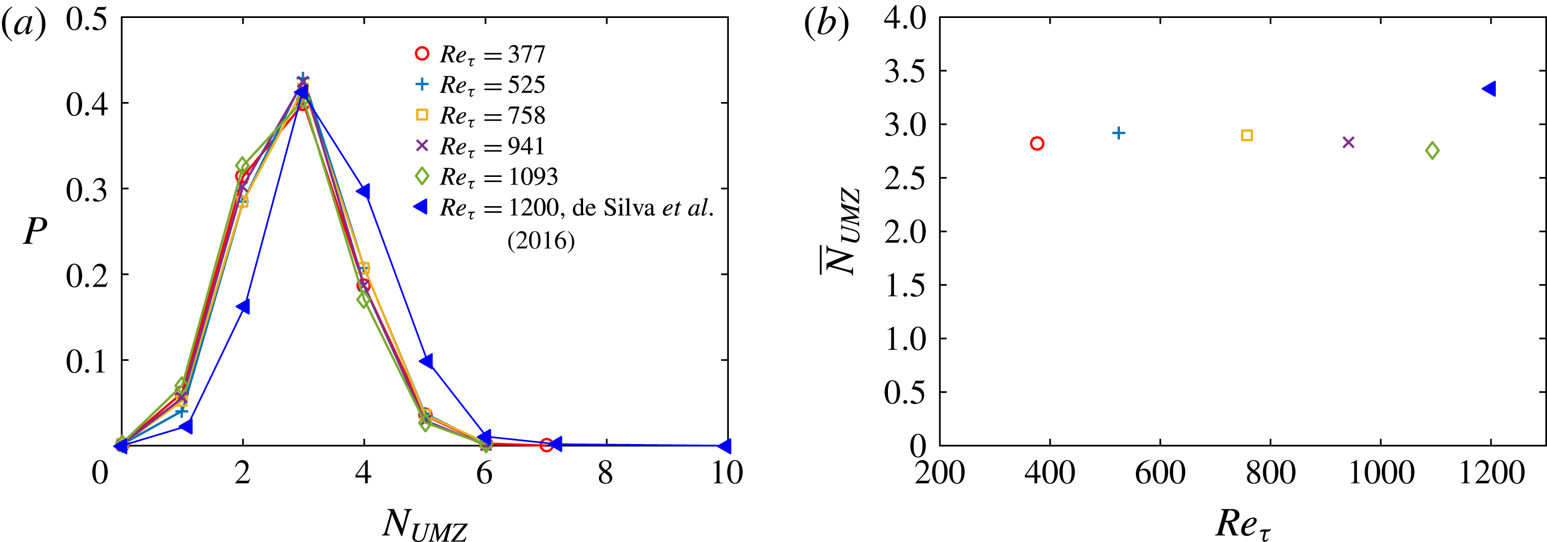
snapshots. Figure 16 shows that both the p.d.f. of the number of UMZs,
 $N_{UMZ}$
, and the mean value,
 $\overline{N}_{UMZ}$
, in the present cases are similar to those at the closest
 $Re_{\unicode[STIX]{x1D70F}}$
(
 $Re_{\unicode[STIX]{x1D70F}}\approx 1200$
) in de Silva et al. (Reference de Silva, Hutchins and Marusic2016).
Note that
 $\overline{N}_{UMZ}$
is always larger than 2 (as shown in figure 16
b), indicating a pattern of multiple IBs (and UMZs) frequently appearing in instantaneous snapshots. In contrast, multiple zero-
 $u^{L}$
lines are seldom observed (see figure 13 for illustration). In the scenario of the coexistence of multi-generations of hairpin packets with various sizes and ages (Adrian Reference Adrian2007), such a difference might be attributed to the fact that zero-
 $u^{L}$
lines are only related to the ‘primary’ hairpin packets, which have the highest TKE contents and are thus mapped onto the leading-order POD modes. On the other hand, the older generations of hairpin packets, although inactive in TKE contribution, still contribute to the formation of UMZs.
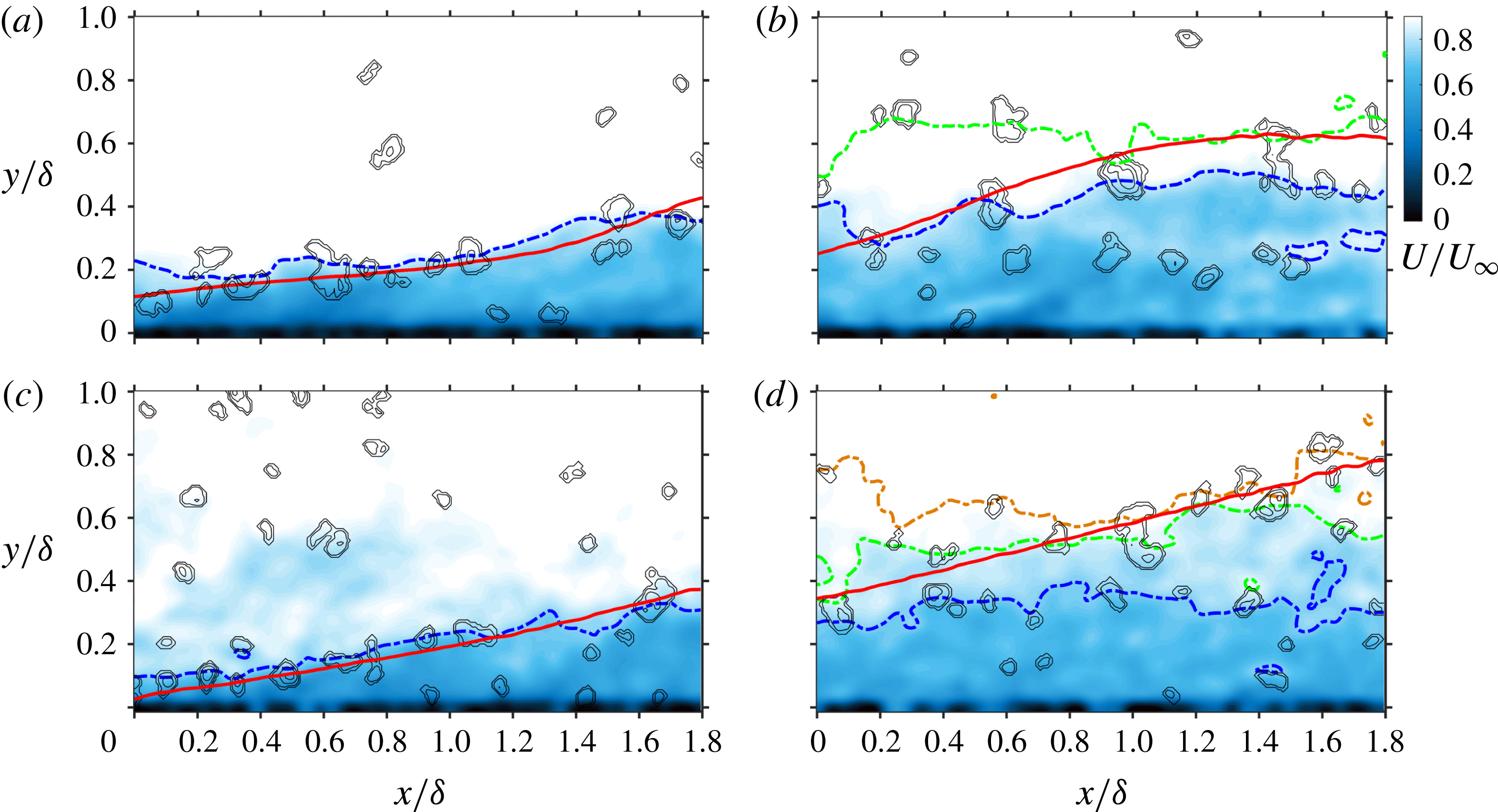
Figure 17 superimposes the zero-
 $u^{L}$
lines onto the instantaneous
 $u$
fields with UMZs being partitioned by IBs. It is clearly shown that, if one snapshot presents only two layers of UMZs with one IB (as shown in figure 17
a,c), there will be a strong spatial coherence between the zero-
 $u^{L}$
line and this IB in the log layer and below; otherwise, the spatial coherence is rather weak (see figure 17
b,d for instance). A further conditional correlation analysis is carried out in appendix A to provide statistical support for this observation.
(a) P.d.f. of the number of UMZs (
 $N_{UMZ}$
), and (b) mean number of UMZs (
 $\overline{N}_{UMZ}$
) as a function of
 $Re_{\unicode[STIX]{x1D70F}}$
: ○,
 $Re_{\unicode[STIX]{x1D70F}}=377$
;
 $+$
,
 $Re_{\unicode[STIX]{x1D70F}}=525$
; ▫,
 $Re_{\unicode[STIX]{x1D70F}}=758$
;
 $\times$
,
 $Re_{\unicode[STIX]{x1D70F}}=941$
; ♢,
 $Re_{\unicode[STIX]{x1D70F}}=1093$
; and ◂,
 $Re_{\unicode[STIX]{x1D70F}}\approx 1200$
in de Silva et al. (Reference de Silva, Hutchins and Marusic2016).

Illustration of the spatial coherence between the zero-
 $u^{L}$
lines and the IBs of the UMZs: (a,b) two snapshots at
 $Re_{\unicode[STIX]{x1D70F}}=377$
; (c,d) two snapshots at
 $Re_{\unicode[STIX]{x1D70F}}=1093$
. Pseudo-colour maps show the full-order streamwise velocity fields
 $U/U_{\infty }$
, bold solid lines are zero-
 $u^{L}$
lines, bold dash-dotted lines are the IBs of the UMZs, and contours indicate regions with concentrated negative
 $\unicode[STIX]{x1D6EC}_{ci}$
.

4.3 Coherence between large-scale interfaces and prograde vortices
According to the hairpin-packet model, the inclined interface should possess a strong spatial coherence with the hairpin heads. This is qualitatively visualized in figure 12, where a large portion of negative
 $\unicode[STIX]{x1D6EC}_{ci}$
concentration regions (with clockwise sense of rotation) are observed to ride on the zero-
 $u^{L}$
lines. Such a picture can be preliminarily examined by studying the p.d.f. of
 $u^{L}$
satisfying the condition
 $\unicode[STIX]{x1D6EC}_{ci}<-\unicode[STIX]{x1D6EC}_{ci}^{\text{T}}$
. Similar to Carlier & Stanislas (Reference Carlier and Stanislas2005) and Herpin et al. (Reference Herpin, Stanislas, Foucaut and Coudert2013), the threshold
 $\unicode[STIX]{x1D6EC}_{ci}^{\text{T}}$
is set as
 $1.5\unicode[STIX]{x1D70E}_{\unicode[STIX]{x1D6EC}}$
, with
 $\unicode[STIX]{x1D70E}_{\unicode[STIX]{x1D6EC}}$
being the r.m.s. value of the local
 $\unicode[STIX]{x1D6EC}_{ci}$
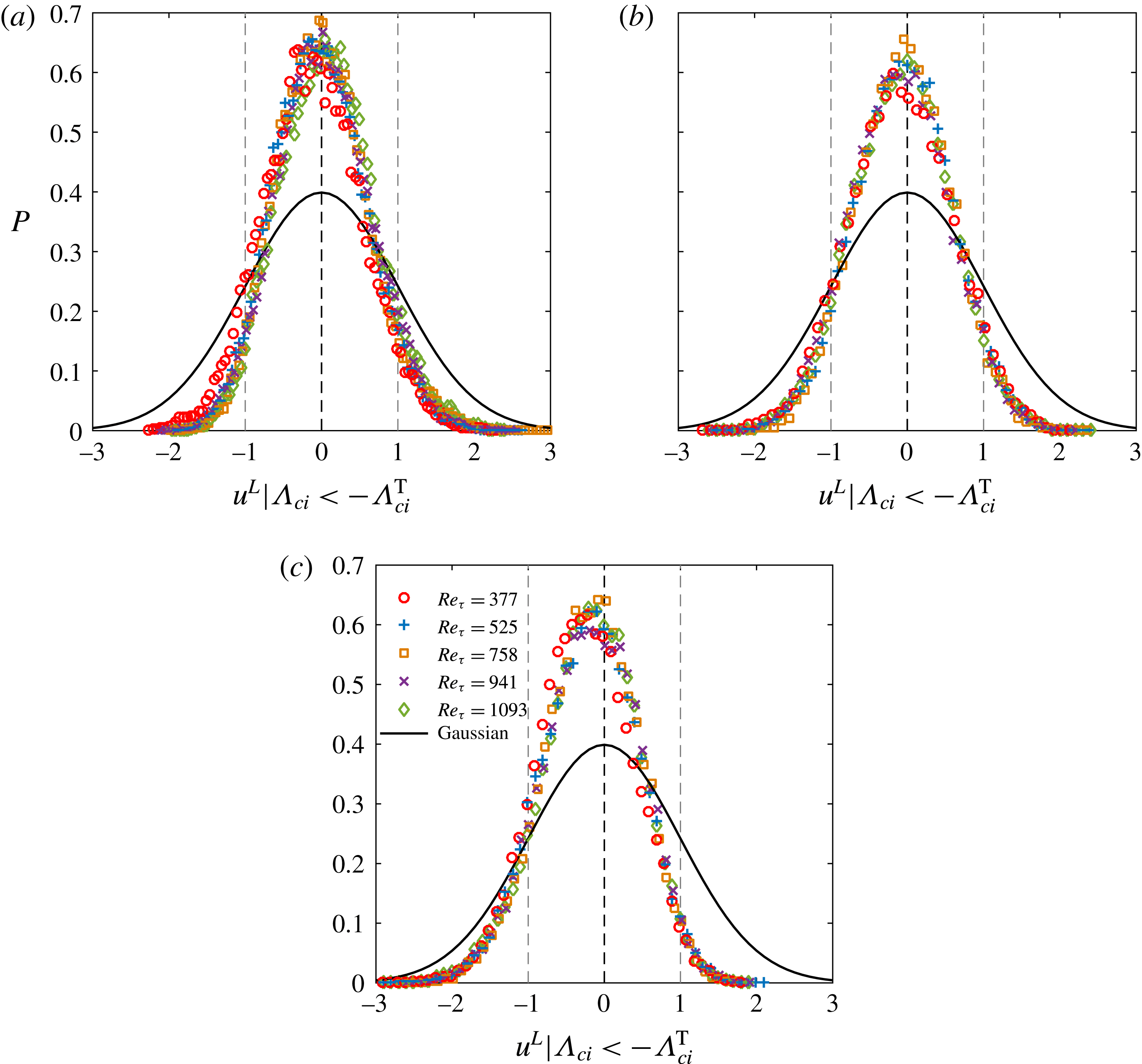
, to guarantee that only the core regions of prograde vortices with sufficient strength are included. Figure 18 shows
 $P(u^{L}/\unicode[STIX]{x1D70E}_{u^{L}}\mid \unicode[STIX]{x1D6EC}_{ci}<-\unicode[STIX]{x1D6EC}_{ci}^{\text{T}})$
at
 $y/\unicode[STIX]{x1D6FF}\approx 0.1$
, 0.3 and 0.5 in all the studied cases, all of which have more compact p.d.f. peaks around
 $u^{L}=0$
than that in a normal distribution. This implies that most of the prograde swirling motions appear in the vicinity of the zero-
 $u^{L}$
lines.
P.d.f. of
 $u^{L}$
satisfying
 $\unicode[STIX]{x1D6EC}_{ci}<-\unicode[STIX]{x1D6EC}_{ci}^{\text{T}}$
at (a)
 $y_{ref}/\unicode[STIX]{x1D6FF}\approx 0.1$
, (b)
 $y_{ref}/\unicode[STIX]{x1D6FF}\approx 0.3$
and (c)
 $y_{ref}/\unicode[STIX]{x1D6FF}\approx 0.5$
: ○,
 $Re_{\unicode[STIX]{x1D70F}}=377$
;
 $+$
,
 $Re_{\unicode[STIX]{x1D70F}}=525$
; ▫,
 $Re_{\unicode[STIX]{x1D70F}}=758$
;
 $\times$
,
 $Re_{\unicode[STIX]{x1D70F}}=941$
; and ♢,
 $Re_{\unicode[STIX]{x1D70F}}=1093$
. Bold solid lines represent the normal distribution. In all the p.d.f. curves,
 $u^{L}$
are normalized by their r.m.s. values
 $\unicode[STIX]{x1D70E}_{u^{L}}$
.

The conditional-averaged
 $u^{L}$
field associated with a strong
 $\unicode[STIX]{x1D6EC}_{ci}$
event is further estimated by linear stochastic estimation (Christensen & Adrian Reference Christensen and Adrian2001):
 $$\begin{eqnarray}\langle u^{L}(r_{x},y)\mid \unicode[STIX]{x1D6EC}_{ci}(x,y_{ref})\rangle \approx L_{u}\unicode[STIX]{x1D6EC}_{ci}(x,y_{ref}),\quad \text{with}~L_{u}=\frac{\langle \unicode[STIX]{x1D6EC}_{ci}(x,y_{ref})u^{L}(x+r_{x},y)\rangle }{\langle \unicode[STIX]{x1D6EC}_{ci}(x,y_{ref})\unicode[STIX]{x1D6EC}_{ci}(x,y_{ref})\rangle }.\end{eqnarray}$$
In (4.1),
 $y_{ref}$
is the reference height,
 $\langle \cdot \rangle$
denotes the average over both the whole snapshot ensemble and the
 $x$
span, while the estimation kernel
 $L_{u}$
differs from
 $\langle u^{L}|\unicode[STIX]{x1D6EC}_{ci}\rangle$
by a factor of
 $\unicode[STIX]{x1D6EC}_{ci}$
. For simplicity, the unconditional two-point correlation
 $R_{\unicode[STIX]{x1D6EC}_{ci}u^{L}}$
is calculated to approximate
 $L_{u}$
:
 $$\begin{eqnarray}R_{\unicode[STIX]{x1D6EC}_{ci}u^{L}}(r_{x},y)=-1\times \frac{\langle \unicode[STIX]{x1D6EC}_{ci}(x,y_{ref})u^{L}(x+r_{x},y)\rangle }{\sqrt{\langle \unicode[STIX]{x1D6EC}_{ci}(x,y_{ref})\unicode[STIX]{x1D6EC}_{ci}(x,y_{ref})\rangle \langle u^{L}(x,y)u^{L}(x,y)\rangle }}.\end{eqnarray}$$
Note that the minus sign in (4.2) is to make the sign of
 $R_{\unicode[STIX]{x1D6EC}_{ci}u^{L}}$
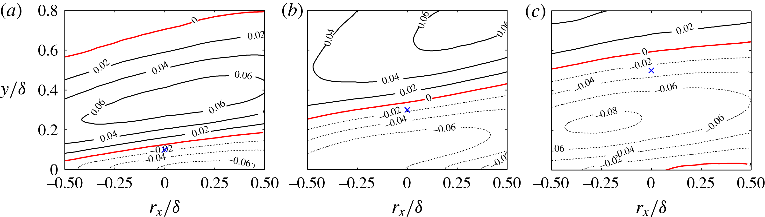
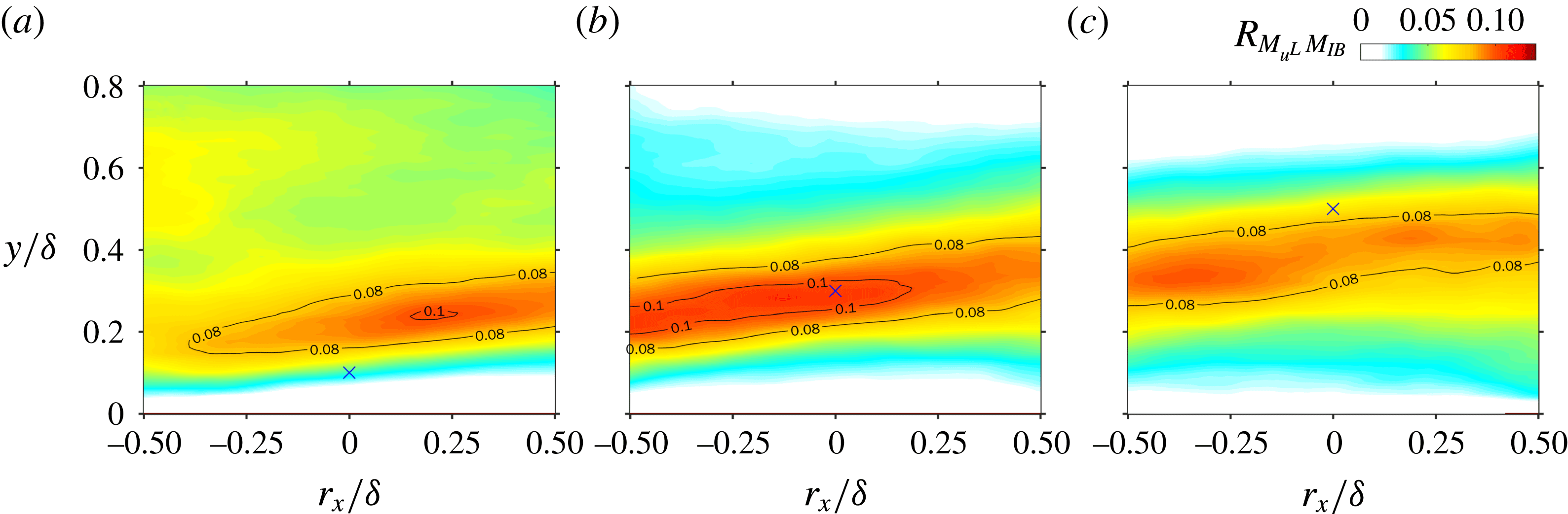
consistent with the converging Q2/Q4 events. Figure 19 plots
 $R_{\unicode[STIX]{x1D6EC}_{ci}u^{L}}$
at
 $y_{ref}/\unicode[STIX]{x1D6FF}\approx 0.1$
, 0.3 and 0.5 in the
 $Re_{\unicode[STIX]{x1D70F}}=1093$
case. Other low-
 $Re$
cases produce similar results and are not presented. A zero-
 $R_{\unicode[STIX]{x1D6EC}_{ci}u^{L}}$
line, which divides the
 $R_{\unicode[STIX]{x1D6EC}_{ci}u^{L}}$
field into the upper positive part and the lower negative part, is always observed above the probing point, providing statistical evidence for the spatial coherence between the large-scale interfaces and the prograde vortices. Moreover, their wall-normal gap increases with
 $y_{ref}$
. This implies that the prograde vortices at higher layer have larger sizes and stronger backward induction to push the interfaces further away, consistent with the self-similar growth of wall-attached eddies in the attached-eddy hypothesis (Townsend Reference Townsend1976; Perry & Chong Reference Perry and Chong1982; Marusic & Perry Reference Marusic and Perry1995; Perry & Marusic Reference Perry and Marusic1995; Marusic & Kunkel Reference Marusic and Kunkel2003). This also explains the observation in figure 18(c) that the most probable peak of
 $P(u^{L}\mid \unicode[STIX]{x1D6EC}_{ci}<-\unicode[STIX]{x1D6EC}_{ci}^{\text{T}})$
at
 $y_{ref}/\unicode[STIX]{x1D6FF}\approx 0.5$
is slightly left offset from
 $u^{L}=0$
.
Two-point correlation map of
 $R_{\unicode[STIX]{x1D6EC}_{ci}u^{L}}(r_{x},y)$
at
 $Re_{\unicode[STIX]{x1D70F}}=1093$
for (a)
 $y_{ref}/\unicode[STIX]{x1D6FF}\approx 0.1$
, (b)
 $y_{ref}/\unicode[STIX]{x1D6FF}\approx 0.3$
and (c)
 $y_{ref}/\unicode[STIX]{x1D6FF}\approx 0.5$
. Solid and light dotted contours represent positive and negative
 $R_{\unicode[STIX]{x1D6EC}_{ci}u^{L}}$
, respectively, bold solid lines are the zero-
 $R_{\unicode[STIX]{x1D6EC}_{ci}u^{L}}$
lines, and cross marks indicate the probing points.

4.4 Conditional correlation analysis of swirling strength
By examining the whole snapshot ensemble, it is found that, in all the studied
 $Re$
cases, more than
 $50\,\%$
of instantaneous
 $\boldsymbol{V}^{L}$
snapshots contain continuous zero-
 $u^{L}$
lines with a streamwise length
 $L_{x}>0.8\unicode[STIX]{x1D6FF}$
. Specifically, a large-scale inclined interface, which can be interpreted as the envelope of one hairpin packet, is a frequently observed event. To further explore the vortex organization within a packet, it is natural to focus on the vicinity of these interfaces. Here, a binarized mask
 $M(x,y)$
is used for this purpose:
 $$\begin{eqnarray}M(x,y)=\left\{\begin{array}{@{}ll@{}}1, & \forall ~(x,y)\in H,\\[2.0pt] 0, & \forall ~(x,y)\notin H,\end{array}\right.H=\{(x,y)\mid y\in [y_{u^{L}=0}\pm \unicode[STIX]{x1D6FF}_{y}]\}.\end{eqnarray}$$
In (4.3),
 $H$
is the neighbouring domain of the inclined interface, determined by shifting the identified zero-
 $u^{L}$
lines along the
 $y$
direction over
 $\pm \unicode[STIX]{x1D6FF}_{y}$
, as illustrated in figure 12. Multiplying
 $\unicode[STIX]{x1D6EC}_{ci}$
by
 $M$
yields the conditional
 $\widetilde{\unicode[STIX]{x1D6EC}}_{ci}$
fields, i.e.
 $\widetilde{\unicode[STIX]{x1D6EC}}_{ci}=M\unicode[STIX]{x1D6EC}_{ci}$
, which mask those swirling motions far away from the inclined interfaces. The two-point correlation of
 $\widetilde{\unicode[STIX]{x1D6EC}}_{ci}$
is then calculated as follows to construct a statistical picture of the vortex organization around the probing point:
 $$\begin{eqnarray}R_{\widetilde{\unicode[STIX]{x1D6EC}}_{ci}\widetilde{\unicode[STIX]{x1D6EC}}_{ci}}(r_{x},y)=\frac{\langle \widetilde{\unicode[STIX]{x1D6EC}}_{ci}(x,y_{ref})\widetilde{\unicode[STIX]{x1D6EC}}_{ci}(x+r_{x},y)\rangle }{\langle \widetilde{\unicode[STIX]{x1D6EC}}_{ci}(x,y_{ref})\widetilde{\unicode[STIX]{x1D6EC}}_{ci}(x,y_{ref})\rangle }.\end{eqnarray}$$
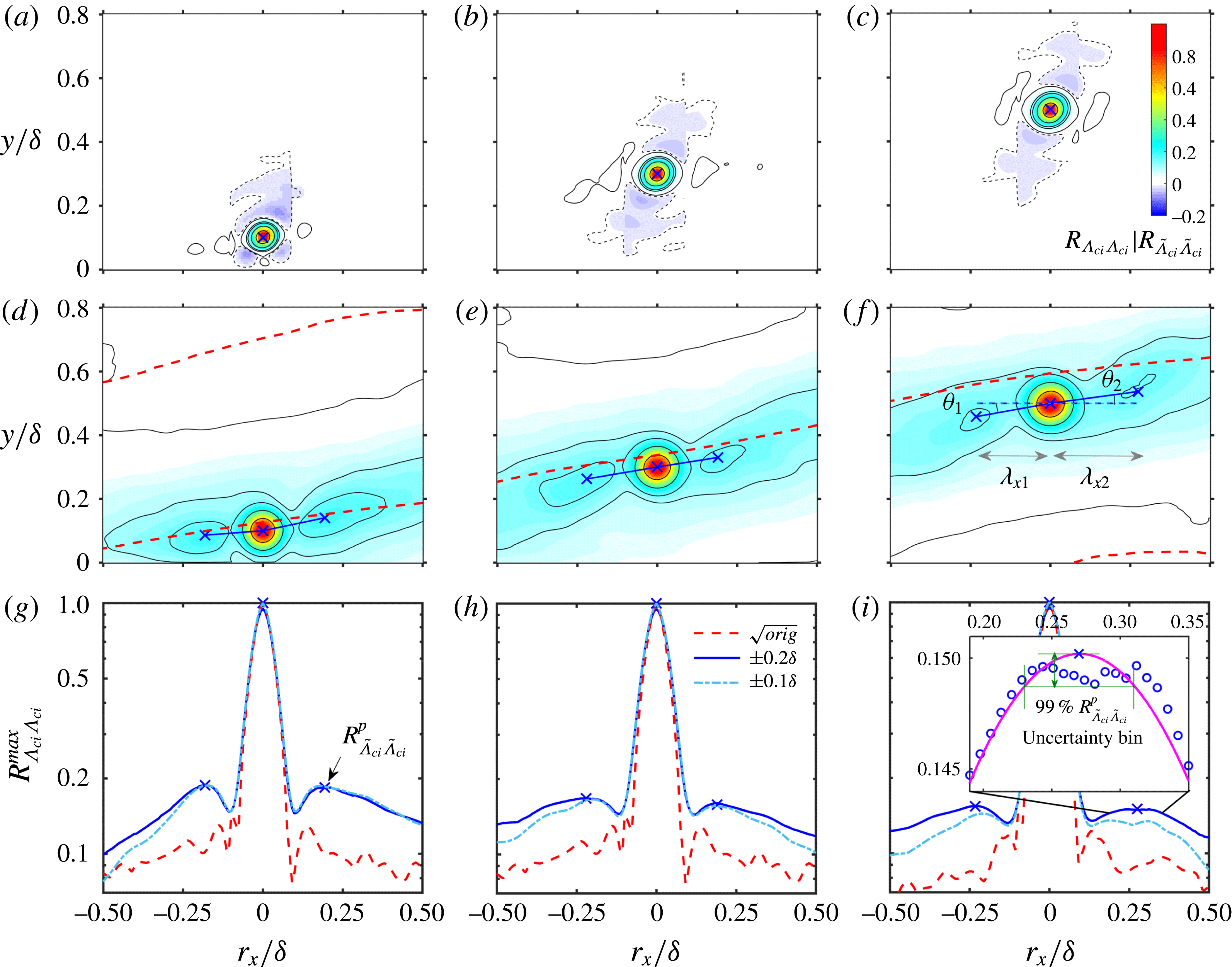
Two-point correlation map
 $R_{\unicode[STIX]{x1D6EC}_{ci}\unicode[STIX]{x1D6EC}_{ci}}$
of the unfiltered
 $\unicode[STIX]{x1D6EC}_{ci}$
fields in (a–c) and
 $R_{\widetilde{\unicode[STIX]{x1D6EC}}_{ci}\widetilde{\unicode[STIX]{x1D6EC}}_{ci}}$
of the filtered
 $\widetilde{\unicode[STIX]{x1D6EC}}_{ci}$
fields in (d–f), together with the streamwise variation of
 $R_{\unicode[STIX]{x1D6EC}_{ci}\unicode[STIX]{x1D6EC}_{ci}}^{max}$
and
 $R_{\widetilde{\unicode[STIX]{x1D6EC}}_{ci}\widetilde{\unicode[STIX]{x1D6EC}}_{ci}}^{max}$
in (g–i), which are the maximum values of the wall-normal profiles
 $R_{\unicode[STIX]{x1D6EC}_{ci}\unicode[STIX]{x1D6EC}_{ci}}(y)$
and
 $R_{\widetilde{\unicode[STIX]{x1D6EC}}_{ci}\widetilde{\unicode[STIX]{x1D6EC}}_{ci}}(y)$
at each
 $r_{x}$
station. Here
 $Re_{\unicode[STIX]{x1D70F}}=1093$
;
 $y_{ref}/\unicode[STIX]{x1D6FF}\approx 0.1$
in (a,d,g);
 $y_{ref}/\unicode[STIX]{x1D6FF}\approx 0.3$
in (b,e,h); and
 $y_{ref}/\unicode[STIX]{x1D6FF}\approx 0.5$
in (c,f,i). The contour levels in (a–f) are (
 $-0.01$
, 0.01, 0.1, 0.15, 0.3, 0.6). In (d–f), the bold dashed lines are the zero-
 $R_{\unicode[STIX]{x1D6EC}_{ci}u^{L}}$
lines shown in figure 19. In (g–i), the dashed lines are the square of the unfiltered
 $R_{\unicode[STIX]{x1D6EC}_{ci}\unicode[STIX]{x1D6EC}_{ci}}^{max}$
, the solid lines are the filtered
 $R_{\widetilde{\unicode[STIX]{x1D6EC}}_{ci}\widetilde{\unicode[STIX]{x1D6EC}}_{ci}}^{max}$
with the mask offset
 $\unicode[STIX]{x1D6FF}_{y}=0.2\unicode[STIX]{x1D6FF}$
, and the dash-dotted lines are
 $R_{\widetilde{\unicode[STIX]{x1D6EC}}_{ci}\widetilde{\unicode[STIX]{x1D6EC}}_{ci}}^{max}$
with
 $\unicode[STIX]{x1D6FF}_{y}=0.1\unicode[STIX]{x1D6FF}$
. The cross marks indicate the secondary correlation peaks
 $R_{\widetilde{\unicode[STIX]{x1D6EC}}_{ci}\widetilde{\unicode[STIX]{x1D6EC}}_{ci}}^{p}$
. The definitions of
 $\unicode[STIX]{x1D703}_{1,2}$
and
 $\unicode[STIX]{x1D706}_{x1,x2}$
to be discussed in § 5.1 are given in (f). The inset of (i) illustrates the uncertainty estimation of both
 $R_{\widetilde{\unicode[STIX]{x1D6EC}}_{ci}\widetilde{\unicode[STIX]{x1D6EC}}_{ci}}^{p}$
and the related
 $\unicode[STIX]{x1D706}_{x1,x2}$
.

The magnitude of the mask offset
 $\unicode[STIX]{x1D6FF}_{y}$
in (4.3) will inevitably affect the resulting
 $R_{\widetilde{\unicode[STIX]{x1D6EC}}_{ci}\widetilde{\unicode[STIX]{x1D6EC}}_{ci}}$
in (4.4). In all the studied cases,
 $\unicode[STIX]{x1D6FF}_{y}$
is selected to be
 $0.2\unicode[STIX]{x1D6FF}$
, sufficiently larger than the radius of most spanwise-rotated vortices (Herpin et al.
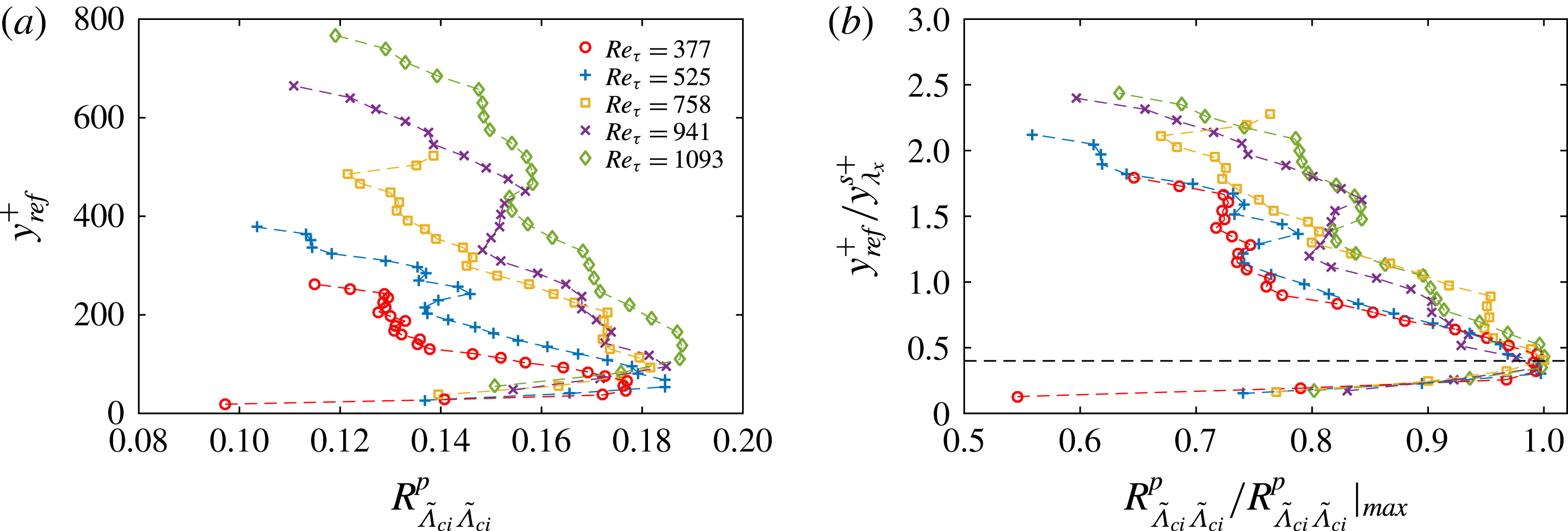
Reference Herpin, Stanislas, Foucaut and Coudert2013). The major consideration in selecting such a large value is to apply a loose constraint to include all the swirling events that are possibly related to the hairpin-packet imprints. In the following discussion on the geometric statistics of the vortex organization (in § 5.1), the peak values in the
 $R_{\widetilde{\unicode[STIX]{x1D6EC}}_{ci}\widetilde{\unicode[STIX]{x1D6EC}}_{ci}}(r_{x},y)$
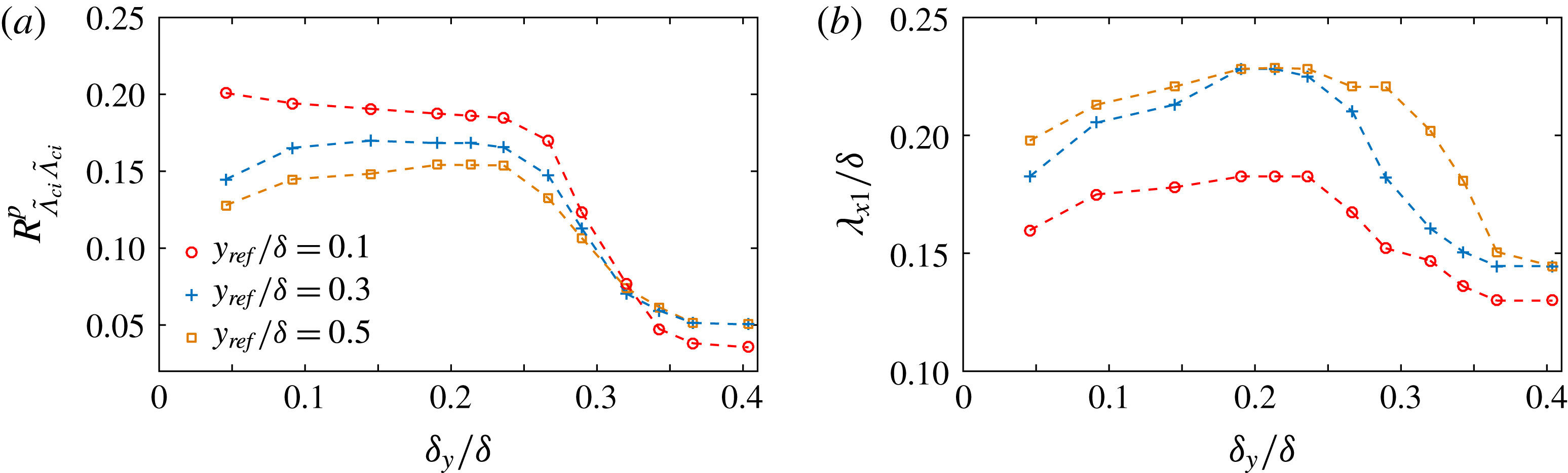
map and the corresponding spatial positions serve as the key parameters. Appendix B uses a systematic test to show that these parameters are rather robust to
 $\unicode[STIX]{x1D6FF}_{y}$
in a range of
 $\unicode[STIX]{x1D6FF}_{y}=(0.10{-}0.25)\unicode[STIX]{x1D6FF}$
.
Figure 20(d–f) gives the map of
 $R_{\widetilde{\unicode[STIX]{x1D6EC}}_{ci}\widetilde{\unicode[STIX]{x1D6EC}}_{ci}}(r_{x},y)$
in the
 $Re_{\unicode[STIX]{x1D70F}}=1093$
case at
 $y_{ref}/\unicode[STIX]{x1D6FF}\approx 0.1$
, 0.3 and 0.5. Other cases with smaller
 $Re$
have similar
 $R_{\widetilde{\unicode[STIX]{x1D6EC}}_{ci}\widetilde{\unicode[STIX]{x1D6EC}}_{ci}}$
maps and are not presented. In addition to the round-shaped autocorrelation region, which represents one spanwise-rotated vortex being probed at
 $r_{x}=0$
and
 $y=y_{ref}$
, two elongated positive
 $R_{\widetilde{\unicode[STIX]{x1D6EC}}_{ci}\widetilde{\unicode[STIX]{x1D6EC}}_{ci}}$
strips (with
 $R_{\widetilde{\unicode[STIX]{x1D6EC}}_{ci}\widetilde{\unicode[STIX]{x1D6EC}}_{ci}}>0.1$
) always appear on both flanks of it. They are in spatial accordance with the zero-
 $R_{\unicode[STIX]{x1D6EC}_{ci}u^{L}}$
lines (red dashed lines in figure 20
d–f) and can be attributed to the scattering distribution of spanwise vortices, whose sense of rotation is the same as that being probed at the autocorrelation peak, along the large-scale Q2/Q4 interfaces. Importantly, secondary peaks
 $R_{\widetilde{\unicode[STIX]{x1D6EC}}_{ci}\widetilde{\unicode[STIX]{x1D6EC}}_{ci}}^{p}$
exist in the
 $R_{\widetilde{\unicode[STIX]{x1D6EC}}_{ci}\widetilde{\unicode[STIX]{x1D6EC}}_{ci}}$
strips (indicated by cross marks in figure 20
d–f). They are highlighted in figure 20(g–i), which plots the streamwise variation of the maximum value of the
 $R_{\widetilde{\unicode[STIX]{x1D6EC}}_{ci}\widetilde{\unicode[STIX]{x1D6EC}}_{ci}}(y)$
profile at each
 $r_{x}$
station. Figure 20(g–i) further shows that, below
 $y_{ref}/\unicode[STIX]{x1D6FF}=0.3$
, a decrease in the mask offset from
 $\unicode[STIX]{x1D6FF}_{y}=0.2$
to
 $\unicode[STIX]{x1D6FF}_{y}=0.1$
will not remarkably affect their magnitudes and spatial positions.
When considering the condition invoked in the conditional correlation scheme, i.e. only the vortices in the vicinity of the large-scale Q2/Q4 interfaces are concerned, the existence of the secondary correlation peaks provides statistical evidence for the hierarchical alignment of multiple prograde vortices within one packet. In contrast, the two-point correlation of the unconditional
 $\unicode[STIX]{x1D6EC}_{ci}$
fields fails to reveal such a picture. As shown in figure 20(a–c), two negative correlation trails are observed on both flanks of the autocorrelation peak, inclining at an angle of about
 $\pm 45^{\circ }$
. Natrajan et al. (Reference Natrajan, Wu and Christensen2007) attributed them to pairs of prograde and retrograde vortices related to the
 $\unicode[STIX]{x03A9}$
-shaped shoulder of hairpin vortices. On the other hand, the positive
 $R_{\widetilde{\unicode[STIX]{x1D6EC}}_{ci}\widetilde{\unicode[STIX]{x1D6EC}}_{ci}}$
strips now degrade to very weak positive
 $R_{\unicode[STIX]{x1D6EC}_{ci}\unicode[STIX]{x1D6EC}_{ci}}$
trails (with the magnitude being less than 0.01) without discernible correlation peaks (as shown in figure 20
g–i). Such a significant difference stresses the necessity of excluding the contamination of irrelevant swirling motions when forming a statistical picture of the vortex organization within a packet.
5 Geometrical description of the vortex organization
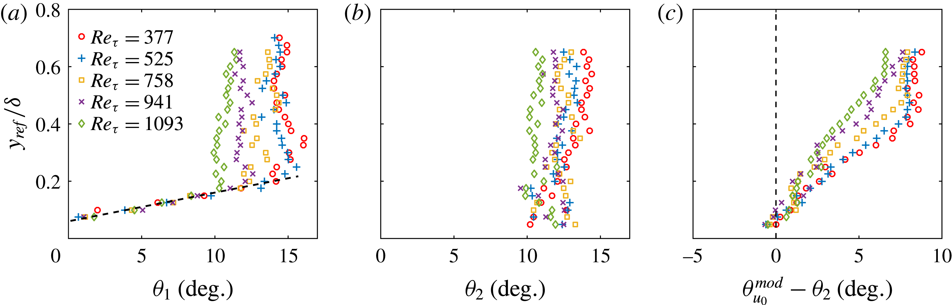
The geometric parameters characterizing the vortex organization are the inclination angles
 $\unicode[STIX]{x1D703}_{1}$
and
 $\unicode[STIX]{x1D703}_{2}$
of the lines connecting two secondary
 $R_{\widetilde{\unicode[STIX]{x1D6EC}}_{ci}\widetilde{\unicode[STIX]{x1D6EC}}_{ci}}$
peaks to the autocorrelation one, as well as their streamwise gaps
 $\unicode[STIX]{x1D706}_{x1}$
and
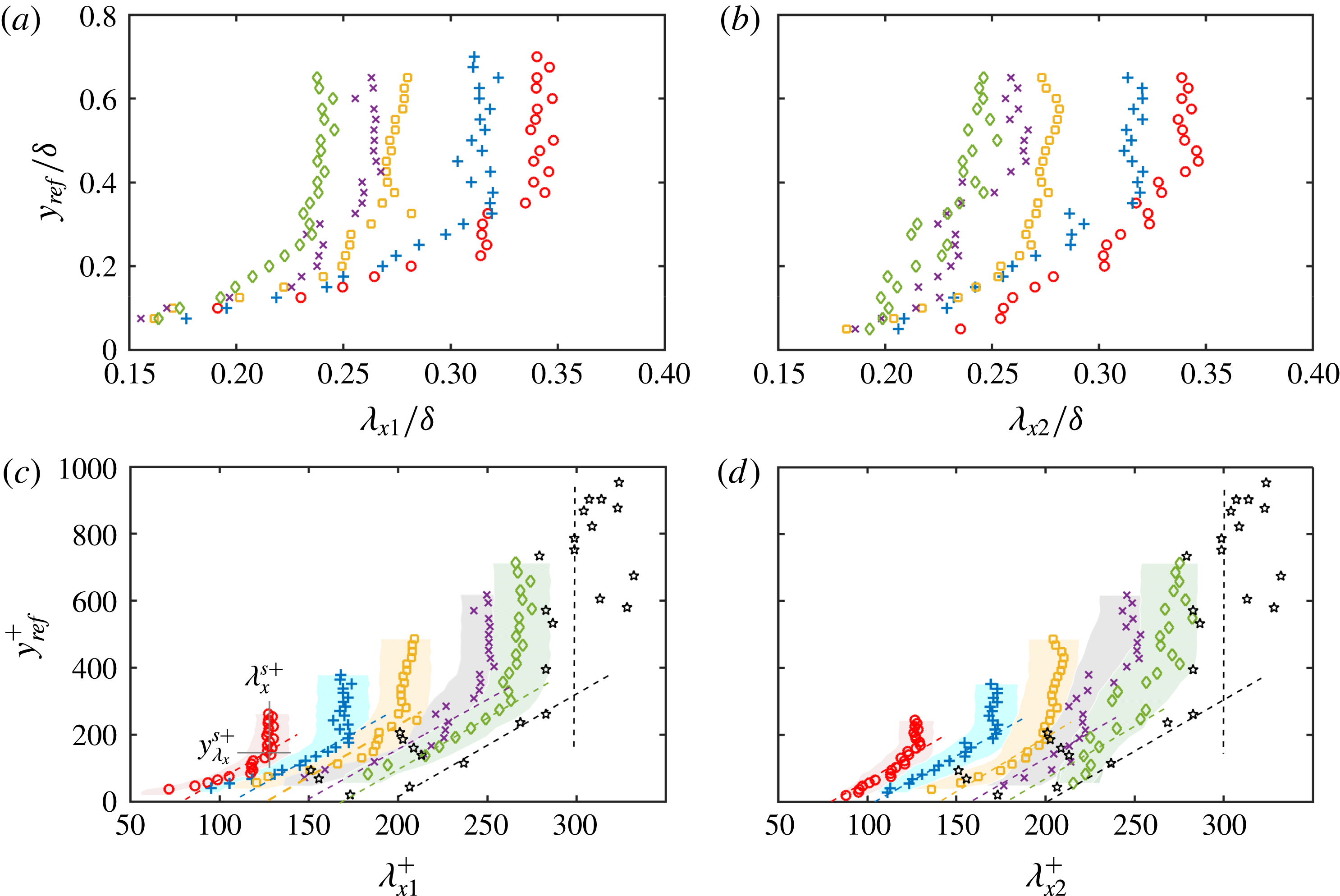
 $\unicode[STIX]{x1D706}_{x2}$
. Figure 20(f) illustrates the definition of these parameters.
To enhance the resolution of
 $\unicode[STIX]{x1D703}_{1,2}$
and
 $\unicode[STIX]{x1D706}_{x1,x2}$
, the spatial positions of the secondary
 $R_{\widetilde{\unicode[STIX]{x1D6EC}}_{ci}\widetilde{\unicode[STIX]{x1D6EC}}_{ci}}$
peaks are refined by localized 2D Gaussian subgrid interpolation. The inset of figure 20(i) gives an illustration in a 1D manner. The figure shows that, even in the worst situation, where a correlation plateau instead of a distinct peak is presented, the Gaussian interpolation remains capable of predicting a ‘pseudo’ peak
 $R_{\widetilde{\unicode[STIX]{x1D6EC}}_{ci}\widetilde{\unicode[STIX]{x1D6EC}}_{ci}}^{p}$
in the middle. It is stressed that such a plateau case only appears in the wake region away from the wall, while a discernible
 $R_{\widetilde{\unicode[STIX]{x1D6EC}}_{ci}\widetilde{\unicode[STIX]{x1D6EC}}_{ci}}^{p}$
(similar to those shown in figure 20
g,h) is always presented in the log layer and below, making the subgrid interpolation rather reliable. The uncertainty of the spatial position of
 $R_{\widetilde{\unicode[STIX]{x1D6EC}}_{ci}\widetilde{\unicode[STIX]{x1D6EC}}_{ci}}^{p}$
(and the uncertainty of
 $\unicode[STIX]{x1D706}_{x1,x2}$
) is estimated by the bin spanning the 99 % range of the predicted
 $R_{\widetilde{\unicode[STIX]{x1D6EC}}_{ci}\widetilde{\unicode[STIX]{x1D6EC}}_{ci}}^{p}$
, as illustrated in the inset of figure 20(i). Note that this is a strict criterion since the yielded uncertainty bin usually spans several grid points or several tens of wall units.
5.1 Wall-normal variation of
 $\unicode[STIX]{x1D703}_{1,2}$
and
$\unicode[STIX]{x1D706}_{x1,x2}$


Figure 21 summarizes
 $\unicode[STIX]{x1D703}_{1}$
and
 $\unicode[STIX]{x1D703}_{2}$
as a function of
 $y_{ref}/\unicode[STIX]{x1D6FF}$
in all the studied cases. A linear wall-normal growth of
 $\unicode[STIX]{x1D703}_{1}$
is always presented below
 $y_{ref}/\unicode[STIX]{x1D6FF}\approx 0.17{-}0.19$
, above which a saturation will be gradually achieved. The larger
 $Re_{\unicode[STIX]{x1D70F}}$
, the lower the flow layer at which the saturation begins. In contrast,
 $\unicode[STIX]{x1D703}_{2}$
is independent of
 $y_{ref}/\unicode[STIX]{x1D6FF}$
. Its magnitude is always larger than that of
 $\unicode[STIX]{x1D703}_{1}$
in the log layer and below, implying a wall-normal steepening of the vortex alignment visualized in figure 20(d). Above the log layer, the magnitudes of
 $\unicode[STIX]{x1D703}_{2}$
and
 $\unicode[STIX]{x1D703}_{1}$
are rather close, all falling in the range of
 $10^{\circ }{-}15^{\circ }$
and being negatively correlated with
 $Re_{\unicode[STIX]{x1D70F}}$
.
Recall that the hairpin-packet model interprets the large-scale interface as a result of the collective backward induction of multiple hairpin vortices. Such a picture can be evaluated by comparing
 $\unicode[STIX]{x1D703}_{2}$
to the most probable inclination angle
 $\unicode[STIX]{x1D703}_{u_{0}}^{mod}$
of the zero-
 $u^{L}$
lines. As shown in figure 21(c),
 $\unicode[STIX]{x1D703}_{u_{0}}^{mod}$
is generally larger than
 $\unicode[STIX]{x1D703}_{2}$
, and the difference between them increases with
 $y_{ref}/\unicode[STIX]{x1D6FF}$
but decreases with
 $Re_{\unicode[STIX]{x1D70F}}$
. In the context of the hairpin-packet model, this observation implies that prograde vortices prefer to align at a shallower angle than that of the inclined interfaces; their backward induction strengths are enhanced at higher flow layer but degrade at higher
 $Re$
.
Wall-normal variation of the averaged inclination angle between neighbouring prograde vortices,
 $\unicode[STIX]{x1D703}_{1}$
in (a) and
 $\unicode[STIX]{x1D703}_{2}$
in (b), as well as the difference between the most probable inclination angle
 $\unicode[STIX]{x1D703}_{u_{0}}^{mod}$
of the zero-
 $u^{L}$
lines and
 $\unicode[STIX]{x1D703}_{2}$
in (c). Symbols: ○,
 $Re_{\unicode[STIX]{x1D70F}}=377$
;
 $+$
,
 $Re_{\unicode[STIX]{x1D70F}}=525$
; ▫,
 $Re_{\unicode[STIX]{x1D70F}}=758$
;
 $\times$
,
 $Re_{\unicode[STIX]{x1D70F}}=941$
; ♢,
 $Re_{\unicode[STIX]{x1D70F}}=1093$
. The definitions of
 $\unicode[STIX]{x1D703}_{1}$
and
 $\unicode[STIX]{x1D703}_{2}$
are illustrated in figure 20(f).

Figure 22 shows the wall-normal variation of
 $\unicode[STIX]{x1D706}_{x1}$
and
 $\unicode[STIX]{x1D706}_{x2}$
in both the outer and inner scaling. Considering the uncertainty bin shown in figure 22(c,d), both
 $\unicode[STIX]{x1D706}_{x1}$
and
 $\unicode[STIX]{x1D706}_{x2}$
present quasi-linear growth in the near-wall region, which are followed by either saturation or very slow variation once
 $y_{ref}$
exceeds a critical height
 $y_{\unicode[STIX]{x1D706}_{x}}^{s}$
(the superscript
 $(\cdot )^{s}$
is short for saturation). Unlike
 $\unicode[STIX]{x1D703}_{1,2}$
, the difference between
 $\unicode[STIX]{x1D706}_{x1}$
and
 $\unicode[STIX]{x1D706}_{x2}$
is rather small. In the inner scaling, the magnitudes of
 $\unicode[STIX]{x1D706}_{x1,x2}^{+}$
monotonically increase with
 $Re_{\unicode[STIX]{x1D70F}}$
, the slopes
 $\unicode[STIX]{x2202}\unicode[STIX]{x1D706}_{x1,x2}^{+}/\unicode[STIX]{x2202}y_{ref}^{+}$
in the linear growth stage are rather close among all the studied cases, and the critical heights
 $y_{\unicode[STIX]{x1D706}_{x}}^{s+}$
are positively correlated with
 $Re_{\unicode[STIX]{x1D70F}}$
. In contrast, none of these features are observed in the outer scaling. The inner-scaled nature of
 $\unicode[STIX]{x1D706}_{x1,x2}$
, in our view, is consistent with the well-known idea that inner-scaled near-wall events are responsible for the generation of packets of vortical structures (Asai et al.
Reference Asai, Minagawa and Nishioka2002; Schoppa & Hussain Reference Schoppa and Hussain2002; Brandt et al.
Reference Brandt, Schlatter and Henningson2004; Brandt & de Lange Reference Brandt and de Lange2008; Wang, Pan & Zhang Reference Wang, Pan and Zhang2009; Jodai & Elsinga Reference Jodai and Elsinga2016; Wu Reference Wu2017).
Wall-normal variation of the averaged streamwise spacing of neighbouring prograde vortices within a packet,
 $\unicode[STIX]{x1D706}_{x1}$
in (a) and (c), and
 $\unicode[STIX]{x1D706}_{x2}$
in (b) and (d): (a) and (b) are the outer-scaling plots, while (c) and (d) are the inner-scaling plots. Symbols: ○,
 $Re_{\unicode[STIX]{x1D70F}}=377$
;
 $+$
,
 $Re_{\unicode[STIX]{x1D70F}}=525$
; ▫,
 $Re_{\unicode[STIX]{x1D70F}}=758$
;
 $\times$
,
 $Re_{\unicode[STIX]{x1D70F}}=941$
; ♢,
 $Re_{\unicode[STIX]{x1D70F}}=1093$
; *,
 $Re_{\unicode[STIX]{x1D70F}}\approx 1141$
in Christensen et al. (Reference Christensen, Wu, Adrian and Lai2004). In (c) and (d), all the inclined dashed lines have the same slope to indicate the quasi-linear growth of
 $\unicode[STIX]{x1D706}_{x1,x2}^{+}$
below
 $y_{\unicode[STIX]{x1D706}_{x}}^{s+}$
. The shaded regions show the uncertainty bins of
 $\unicode[STIX]{x1D706}_{x1,x2}^{+}$
estimated via a
 $99\,\%$
 $R_{\widetilde{\unicode[STIX]{x1D6EC}}_{ci}\widetilde{\unicode[STIX]{x1D6EC}}_{ci}}^{p}$
criterion illustrated in figure 20(i), which indicates a full separation of
 $\unicode[STIX]{x1D706}_{x1,x2}^{+}$
among the four smallest
 $Re$
cases. The definitions of
 $\unicode[STIX]{x1D706}_{x1}$
and
 $\unicode[STIX]{x1D706}_{x2}$
are illustrated in figure 20(f), and the definitions of
 $\unicode[STIX]{x1D706}_{x}^{s+}$
and
 $y_{\unicode[STIX]{x1D706}_{x}}^{s+}$
are given in figure 22(c).

5.2 Discussion of the
$Re$
dependence of
$\unicode[STIX]{x1D706}_{x1,x2}$


Christensen et al. (Reference Christensen, Wu, Adrian and Lai2004) reported a logarithmic wall-normal growth of the mean streamwise spacing of neighbouring prograde vortices, which were regarded by them as the hairpin heads. This conflicts with the quasi-linear growth of
 $\unicode[STIX]{x1D706}_{x1,x2}^{+}$
and the subsequent saturation observed here. For a comparison, the data of
 $\unicode[STIX]{x1D706}_{x}^{+}\sim y^{+}$
at
 $Re_{\unicode[STIX]{x1D70F}}\approx 1141$
in Christensen et al. (Reference Christensen, Wu, Adrian and Lai2004) are reproduced in figure 22(c,d). Despite the remarkable scattering of
 $\unicode[STIX]{x1D706}_{x}^{+}$
, which can be attributed to the large uncertainty of the acceleration measurement in Christensen et al. (Reference Christensen, Wu, Adrian and Lai2004), a saturation of
 $\unicode[STIX]{x1D706}_{x}^{+}$
seems to be presented in the outer region if abnormal data are omitted. Meanwhile, the near-wall part of
 $\unicode[STIX]{x1D706}_{x}^{+}\sim y^{+}$
in Christensen et al. (Reference Christensen, Wu, Adrian and Lai2004) can be reasonably characterized by a liner correlation.
The
 $Re$
dependence of (a) the saturated
 $\unicode[STIX]{x1D706}_{x}^{s+}$
and (b) the corresponding detachment height
 $y_{\unicode[STIX]{x1D706}_{x}}^{s+}$
. In (a), symbols are: ○,
 $\unicode[STIX]{x1D706}_{x1}^{s+}$
;
 $+$
,
 $\unicode[STIX]{x1D706}_{x2}^{s+}$
; ▫,
 $\unicode[STIX]{x1D706}_{x}^{s+}$
in Christensen et al. (Reference Christensen, Wu, Adrian and Lai2004) with error bar indicating the r.m.s. value in the slow variation stage. In (b), symbols are: ○,
 $y_{\unicode[STIX]{x1D706}_{x1}}^{s+}$
;
 $+$
,
 $y_{\unicode[STIX]{x1D706}_{x2}}^{s+}$
. The solid straight lines in (a) and (b) indicate a
 $Re_{\unicode[STIX]{x1D70F}}^{1/2}$
scaling, and the dashed line in (b) shows a
 $y_{M}^{+}=3.9Re_{\unicode[STIX]{x1D70F}}^{1/2}$
formulation (Mathis, Hutchins & Marusic Reference Mathis, Hutchins and Marusic2009) suggesting the geometric centre of the log layer.

The quasi-linear growth of
 $\unicode[STIX]{x1D706}_{x1,x2}^{+}$
below
 $y_{\unicode[STIX]{x1D706}_{x}}^{s+}$
implies a self-similarity of the streamwise spacing of neighbouring vortices within one packet, which is consistent with the linear growth of the length scales of conditional eddies associated with hairpin vortices (Tomkins & Adrian Reference Tomkins and Adrian2003; Dennis & Nickels Reference Dennis and Nickels2011). Meanwhile, the saturation of
 $\unicode[STIX]{x1D706}_{x1,x2}^{+}$
beyond
 $y_{\unicode[STIX]{x1D706}_{x}}^{s+}$
indicates a detachment of this self-similar growth. As shown in figure 23(a), the saturated
 $\unicode[STIX]{x1D706}_{x1,x2}^{s+}$
, which are measured by the mean value of
 $\unicode[STIX]{x1D706}_{x1,x2}^{+}$
beyond
 $y_{\unicode[STIX]{x1D706}_{x}}^{s+}$
, follows a
 $Re_{\unicode[STIX]{x1D70F}}^{1/2}$
scaling. The saturated
 $\unicode[STIX]{x1D706}_{x}^{s+}$
in the dataset of Christensen et al. (Reference Christensen, Wu, Adrian and Lai2004) are estimated in a similar manner: (1) low-pass filtering the
 $\unicode[STIX]{x1D706}_{x}^{+}\sim y^{+}$
curve, with abnormal points being manually removed in advance; and (2) calculating the average value and the r.m.s. value of the low-pass-filtered
 $\unicode[STIX]{x1D706}_{x}^{+}$
in the region with slow wall-normal variation as
 $\unicode[STIX]{x1D706}_{x}^{s+}$
and its uncertainty, respectively. As shown in figure 23(a), the estimated
 $\unicode[STIX]{x1D706}_{x}^{s+}$
in Christensen et al. (Reference Christensen, Wu, Adrian and Lai2004), despite the rather large uncertainty, shows a reasonable agreement with the present
 $Re_{\unicode[STIX]{x1D70F}}^{1/2}$
scaling.
Wu & Christensen (Reference Wu and Christensen2006) reported a
 $Re_{\unicode[STIX]{x1D70F}}^{-1/2}$
scaling of the inner-scaled population density
 $\unicode[STIX]{x1D6F1}_{p}^{+}$
of prograde vortices. Referring to the definition of
 $\unicode[STIX]{x1D6F1}_{p}^{+}$
, which measures the average number of detected prograde vortices per unit area at one wall-normal height, the
 $\unicode[STIX]{x1D6F1}_{p}^{+}\sim Re_{\unicode[STIX]{x1D70F}}^{-1/2}$
correlation implies a
 $Re_{\unicode[STIX]{x1D70F}}^{1/2}$
dependence of the averaged streamwise gap between two neighbouring prograde vortices, consistent with the present scaling of
 $\unicode[STIX]{x1D706}_{x1,x2}^{s+}\sim Re_{\unicode[STIX]{x1D70F}}^{1/2}$
.
Furthermore, in the concept of the intermediate meso-layer (Sreenivasan Reference Sreenivasan1989; Klewicki et al.
Reference Klewicki, Fife and Wei2009), the location
 $y_{RSmax}^{+}$
of the maximum Reynolds stress scales with
 $Re_{\unicode[STIX]{x1D70F}}^{1/2}$
. Morrison et al. (Reference Morrison, McKeon, Jiang and Smits2004) assumed that the magnitude of the maximum RSS scales approximately with
 $Re_{\unicode[STIX]{x1D70F}}^{1/2}$
in pipe flows. Eyink (Reference Eyink2008) derived a
 $Re_{\unicode[STIX]{x1D70F}}^{1/2}$
dependence of the location of the maximum RSS by a modified attached-eddy approach. In addition, Alfredsson, Segalini & Orlu (Reference Alfredsson, Segalini and Orlu2011) proposed that the wall-normal height
 $y_{u,max}^{+}$
of the outer
 $u_{rms}$
peak scales with
 $Re_{\unicode[STIX]{x1D70F}}^{0.56}$
by
 $y_{u,max}^{+}=0.81Re_{\unicode[STIX]{x1D70F}}^{0.56}$
.
In the present case, the near-wall quasi-linear growth of
 $\unicode[STIX]{x1D706}_{x1,x2}^{+}$
and the
 $Re_{\unicode[STIX]{x1D70F}}^{1/2}$
dependence of
 $\unicode[STIX]{x1D706}_{x1,x2}^{s+}$
lead to a
 $Re_{\unicode[STIX]{x1D70F}}^{1/2}$
scaling of
 $y_{\unicode[STIX]{x1D706}_{x}}^{s+}$
. This is evidenced by figure 23(b), in which
 $y_{\unicode[STIX]{x1D706}_{x}}^{s+}$
is estimated as the wall-normal position where
 $\unicode[STIX]{x2202}\unicode[STIX]{x1D706}_{x1,x2}^{+}/\unicode[STIX]{x2202}y_{ref}^{+}$
presents a sharp drop. The data of Christensen et al. (Reference Christensen, Wu, Adrian and Lai2004) are not included due to the difficulty in precisely estimating
 $y_{\unicode[STIX]{x1D706}_{x}}^{s+}$
in their case. A relation of
 $y_{M}^{+}=3.9Re_{\unicode[STIX]{x1D70F}}^{1/2}$
, which was proposed by Mathis et al. (Reference Mathis, Hutchins and Marusic2009) to formulate the geometric centre of the log layer, is also provided in figure 23(b) (as dashed line). Clearly, the saturation of
 $\unicode[STIX]{x1D706}_{x1,x2}^{+}$
occurs above the centre of the log layer, where a secondary
 $u_{rms}$
peak is expected under high-
 $Re$
condition (Mathis et al.
Reference Mathis, Hutchins and Marusic2009). The locations of
 $y_{\unicode[STIX]{x1D706}_{x}}^{s+}$
are further superimposed onto the
 $u_{rms}^{+}(y^{+})$
profiles in figure 1(b). This gives a hint that
 $y_{\unicode[STIX]{x1D706}_{x}}^{s+}$
locates at the right end of the ‘shoulder’ of the
 $u_{rms}^{+}(y^{+})$
profile (due to the low-to-moderate
 $Re$
, no outer
 $u_{rms}$
peak is observed here), beyond which
 $u_{rms}$
presents a quick drop. Such an observation suggests that
 $y_{\unicode[STIX]{x1D706}_{x}}^{s+}$
is related to the commencement of the intermediate meso-layer, above which the hairpin packets generated by the near-wall events gradually detach from the wall and become less active in contributing to the streamwise turbulent fluctuations.
6 Concluding remarks
In summary, the present study performs the following analysis to form a statistical picture of the coherent organization of vortical structures from 2D PIV measured velocity fields in the streamwise–wall-normal plane of a canonical turbulent boundary layer at low-to-moderate
 $Re$
.
A spatio-temporal coherence analysis of the energy-containing POD modes, similar to that in Hellström & Smits (Reference Hellström and Smits2014) and Hellström et al. (Reference Hellström, Ganapathisubramani and Smits2015), is first conducted to show that the first four leading-order POD modes jointly depict the downstream convection of the large-scale converging Q2/Q4 events, which are believed to be the low-order representatives of the large-scale imprints of the hairpin packets. The zero-
 $u^{L}$
lines detected in the low-order reconstructed fields are then used as the indicators of the inclined interfaces between the hairpin packets and the environment flow. In the near-wall region, these zero-
 $u^{L}$
lines are found to pose strong spatial coherence with the IBs of the UMZs (de Silva et al.
Reference de Silva, Hutchins and Marusic2016). Linear stochastic estimation shows that small-scale prograde vortices in the full-order fields prefer to reside on them. Finally, the conditional two-point correlation map
 $R_{\widetilde{\unicode[STIX]{x1D6EC}}_{ci}\widetilde{\unicode[STIX]{x1D6EC}}_{ci}}$
of the swirling strength fields
 $\widetilde{\unicode[STIX]{x1D6EC}}_{ci}$
, in which those spanwise swirling motions being less relevant to the zero-
 $u^{L}$
lines are excluded, reveals a statistical picture of three streamwise-aligned prograde vortices beneath one large-sale inclined interface, consistent with the paradigm of the hairpin-packet model. Note that such a pattern cannot be obtained by the unconditional correlation analysis; this highlights the necessity of focusing on the neighbourhood of the zero-
 $u^{L}$
lines.
It is stressed that the above analysis cannot be regarded as a ‘generalized’ scheme for the statistical depiction of turbulent coherent structures. This is because the selection of several key parameters, i.e. the number of leading-order modes being grouped for the low-order representation and the mask offset
 $\unicode[STIX]{x1D6FF}_{y}$
in constructing
 $R_{\widetilde{\unicode[STIX]{x1D6EC}}_{ci}\widetilde{\unicode[STIX]{x1D6EC}}_{ci}}$
(in (4.3) and (4.4)), relies on either experience or trial-and-error testing. Nevertheless, the presently obtained geometrical statistics, i.e. the inclination angle
 $\unicode[STIX]{x1D703}_{1,2}$
and the streamwise gap
 $\unicode[STIX]{x1D706}_{x1,x2}$
between two neighbouring prograde vortices in a packet, are believed to be rather reliable. The justification lies in the following aspects. First, the first four leading-order POD modes are insensitive to
 $Re$
and FOV, as shown in § 3.1. Second, both § 4.4 and appendix B demonstrate that
 $R_{\widetilde{\unicode[STIX]{x1D6EC}}_{ci}\widetilde{\unicode[STIX]{x1D6EC}}_{ci}}$
are robust to
 $\unicode[STIX]{x1D6FF}_{y}$
. Finally, § 5.1 shows that the uncertainties of estimating
 $\unicode[STIX]{x1D706}_{x1,x2}^{+}$
will not change the variation trend of
 $\unicode[STIX]{x1D706}_{x1,x2}$
with both
 $y/\unicode[STIX]{x1D6FF}$
and
 $Re$
. Comparing to the IB of the UMZs, the zero-
 $u^{L}$
line has a much simpler mathematical definition and is regarded as a more suitable indicator of the interfaces of those energy-containing hairpin packets. In later studies, a similar conditional correlation can be taken to identify the averaged vortical structures associated with the IBs of the UMZs.
One of the most interesting findings in the present study is that the inner-scaled
 $\unicode[STIX]{x1D706}_{x1,x2}^{+}$
increases with
 $Re$
. In the context of the hairpin-packet model, a larger spacing results in a weaker cooperative induction strength of individual vortices in the packet. This suggests a higher possibility that the coherence between neighbouring vortices is apt to be destroyed by random turbulent fluctuations. Whether this offers a possible explanation for the debate on the existence of hairpin forest/packets under moderate-to-high
 $Re$
condition (Schlatter & Orlu Reference Schlatter and Orlu2010; Sayadi et al.
Reference Sayadi, Hamman and Moin2013; Schlatter et al.
Reference Schlatter, Li, Orlu, Hussain and Henningson2014; Wu et al.
Reference Wu, Moin and Hickey2014; Eitel-Amor et al.
Reference Eitel-Amor, Orlu, Schlatter and Flores2015) deserves to be studied in the future.
Finally,
 $\unicode[STIX]{x1D706}_{x1,x2}^{+}$
presents a detachment from the near-wall self-similar growth beyond a critical layer of
 $y_{\unicode[STIX]{x1D706}_{x}}^{s+}$
, which seems to be related to the quick drop of the streamwise turbulent fluctuation. In the future, the observed
 $Re_{\unicode[STIX]{x1D70F}}^{1/2}$
scaling of
 $y_{\unicode[STIX]{x1D706}_{x}}^{s+}$
needs to be validated in high-
 $Re$
scenarios, together with a detailed discussion on the relationship between this detachment layer and the intermediate meso-layer (Sreenivasan Reference Sreenivasan1989; Klewicki et al.
Reference Klewicki, Fife and Wei2009).
Acknowledgements
This work was supported by both the National Natural Science Foundation of China (grant nos. 11490552, 11672020 and 11721202) and the Fundamental Research Funds for the Central Universities of China (no. YWF-16-JCTD-A-05).
Supplementary movie
Supplementary movie is available at https://doi.org/10.1017/jfm.2018.160.
Appendix A. Correlation between zero-
$u^{L}$
lines and IBs of UMZs

A conditional correlation is constructed here to characterize the spatial relationship between the zero-
 $u^{L}$
lines and the IBs of the UMZs. Owing to the observation in § 4.2, only the first-layer IBs closest to the wall, which are possible to be correlated with the zero-
 $u^{L}$
lines, are considered here.
The correlation is taken between the binarized masks accounting for a narrow neighbourhood around these two characteristic lines, similar to the conditional correlation of (4.3) and (4.4) in § 4.4. For one snapshot, the binarized mask
 $M_{u^{L}}$
of the zero-
 $u^{L}$
lines is
 $$\begin{eqnarray}M_{u^{L}}(x,y)=\left\{\begin{array}{@{}ll@{}}1, & \forall ~(x,y)\in H_{u^{L}},\\[2.0pt] 0, & \forall ~(x,y)\notin H_{u^{L}},\end{array}\right.H_{u^{L}}=\{(x,y)\mid y\in [y_{u^{L}=0}\pm 0.02\unicode[STIX]{x1D6FF}]\},\end{eqnarray}$$
which is a wall-normal shift of the detected zero-
 $u^{L}$
line over
 $\pm 0.02\unicode[STIX]{x1D6FF}_{y}$
(spanning approximately
 $2{-}3$
grid points). The binarized mask
 $M_{IB}$
of the IBs is
 $$\begin{eqnarray}\displaystyle & & \displaystyle \!\!\!\!\!M_{IB}(x,y)\nonumber\\ \displaystyle & & \displaystyle \!\!\!\!\!~=\left\{\begin{array}{@{}ll@{}}1, & \forall ~(x,y)\in H_{IB},\\[2.0pt] 0, & \forall ~(x,y)\notin H_{IB},\end{array}\right.H_{IB}=\{(x,y)\mid y\in [y_{U=U_{mid}}\pm 0.05\unicode[STIX]{x1D6FF}]\cap U(x,y)\in [(1\pm 10\,\%)U_{mid}]\},\hspace{-3.0pt}\nonumber\\ \displaystyle & & \displaystyle\end{eqnarray}$$
in which only the first-layer IBs are included, the shift width is relaxed to
 $0.05\unicode[STIX]{x1D6FF}_{y}$
, and an additional constraint stating that the local streamwise velocity
 $U$
should not differ too much from
 $U_{mid}$
, the mid-point between modal velocities of neighbouring UMZs, is also imposed.
The correlation of
 $M_{u^{L}}$
to
 $M_{IB}$
takes the form
 $$\begin{eqnarray}R_{M_{u^{L}}M_{IB}}(r_{x},y)=\frac{\langle M_{u^{L}}(x,y_{ref})M_{IB}(x+r_{x},y)\rangle }{\sqrt{\langle M_{u^{L}}(x,y_{ref})M_{u^{L}}(x,y_{ref})\rangle \langle M_{IB}(x,y)M_{IB}(x,y)\rangle }}.\end{eqnarray}$$
This yields an estimation of the averaged shape of the IBs associated with one zero-
 $u^{L}$
event. The larger the neighbourhood being included, the higher the magnitude of
 $R_{M_{u^{L}}M_{IB}}$
yielded. For strict criteria, the shift widths in (A 1) and (A 2) are set to be as small as possible.
Figure 24 illustrates the typical correlation map
 $R_{M_{u^{L}}M_{IB}}(r_{x},y)$
at
 $Re_{\unicode[STIX]{x1D70F}}=1093$
, which indicates a strong spatial coherence between the zero-
 $u^{L}$
lines and the first-layer IBs in the near-wall region. A satisfying overlap of these two characteristic lines appears around
 $y/\unicode[STIX]{x1D6FF}\approx 0.2{-}0.3$
, above which a decorrelation is observed, with the maximum value of
 $R_{M_{u^{L}}M_{IB}}$
quickly dropping below 0.1. Other smaller
 $Re$
cases produce the same finding. Moreover, it has been tested that, if all the layers of IBs are included, the correlation peaks of
 $R_{M_{u^{L}}M_{IB}}$
never exceed 0.1 (not shown here), in accordance with the visualization in figure 17 that only the first-layer IBs of the UMZs are in spatial coherence with the zero-
 $u^{L}$
lines.
Two-point correlation map of
 $R_{M_{u^{L}}M_{IB}}(r_{x},y)$
: (a)
 $y_{ref}/\unicode[STIX]{x1D6FF}\approx 0.1$
; (b)
 $y_{ref}/\unicode[STIX]{x1D6FF}\approx 0.3$
; and (c)
 $y_{ref}/\unicode[STIX]{x1D6FF}\approx 0.5$
. The cross marks indicate the probing points. Here
 $Re_{\unicode[STIX]{x1D70F}}=1093$
.

Appendix B. Robustness of the conditional correlation analysis
In § 4.4,
 $\unicode[STIX]{x1D6EC}_{ci}$
is masked by the neighbourhood of the zero-
 $u^{L}$
lines before the correlation calculation in (4.4). The mask offset
 $\unicode[STIX]{x1D6FF}_{y}$
in the construction of the binarized mask
 $M$
in (4.3) is a critical parameter that affects the yielded correlation map
 $R_{\widetilde{\unicode[STIX]{x1D6EC}}_{ci}\widetilde{\unicode[STIX]{x1D6EC}}_{ci}}(r_{x},y)$
. Nevertheless, figure 25 shows that both the magnitude of the left-side secondary correlation peak
 $R_{\widetilde{\unicode[STIX]{x1D6EC}}_{ci}\widetilde{\unicode[STIX]{x1D6EC}}_{ci}}^{p}$
and its streamwise gap
 $\unicode[STIX]{x1D706}_{x1}$
to the central autocorrelation peak are less sensitive to
 $\unicode[STIX]{x1D6FF}_{y}$
in the range of
 $\unicode[STIX]{x1D6FF}_{y}/\unicode[STIX]{x1D6FF}\approx 0.1{-}0.25$
at
 $Re_{\unicode[STIX]{x1D70F}}=1093$
. Such a weak
 $\unicode[STIX]{x1D6FF}_{y}$
dependence is also observed in the right-side secondary correlation peak. It persists in the outer region (until
 $y_{ref}/\unicode[STIX]{x1D6FF}\approx 0.5$
) and also holds for other lower
 $Re$
cases (not presented here). Combining with figure 20(g–i), which compares the profiles of
 $R_{\widetilde{\unicode[STIX]{x1D6EC}}_{ci}\widetilde{\unicode[STIX]{x1D6EC}}_{ci}}^{max}(r_{x})$
with
 $\unicode[STIX]{x1D6FF}_{y}/\unicode[STIX]{x1D6FF}=0.2$
and 0.1, it can be concluded that
 $\unicode[STIX]{x1D6FF}_{y}=0.2\unicode[STIX]{x1D6FF}$
used in § 4.4 yields a stable statistical description of the vortex organization.
Effect of the mask offset
 $\unicode[STIX]{x1D6FF}_{y}$
on (a) the magnitude
 $R_{\widetilde{\unicode[STIX]{x1D6EC}}_{ci}\widetilde{\unicode[STIX]{x1D6EC}}_{ci}}^{p}$
of the left-side secondary correlation peak and (b) its streamwise gap
 $\unicode[STIX]{x1D706}_{x1}$
to the central autocorrelation peak. Symbols: ○,
 $y_{ref}/\unicode[STIX]{x1D6FF}\approx 0.1$
;
 $+$
,
 $y_{ref}/\unicode[STIX]{x1D6FF}\approx 0.3$
; ▫,
 $y_{ref}/\unicode[STIX]{x1D6FF}\approx 0.5$
. Here
 $Re_{\unicode[STIX]{x1D70F}}=1093$
.

(a) Wall-normal variation of the magnitude
 $R_{\widetilde{\unicode[STIX]{x1D6EC}}_{ci}\widetilde{\unicode[STIX]{x1D6EC}}_{ci}}^{p}$
of the left-side secondary correlation peak with
 $\unicode[STIX]{x1D6FF}_{y}=0.2\unicode[STIX]{x1D6FF}$
. (b) The same curves but with
 $R_{\widetilde{\unicode[STIX]{x1D6EC}}_{ci}\widetilde{\unicode[STIX]{x1D6EC}}_{ci}}^{p}$
being normalized by
 $R_{\widetilde{\unicode[STIX]{x1D6EC}}_{ci}\widetilde{\unicode[STIX]{x1D6EC}}_{ci}}^{p}\big|_{max}$
and
 $y_{ref}^{+}$
being normalized by
 $y_{\unicode[STIX]{x1D706}_{x}}^{s+}$
. Symbols: ○,
 $Re_{\unicode[STIX]{x1D70F}}=377$
;
 $+$
,
 $Re_{\unicode[STIX]{x1D70F}}=525$
; ▫,
 $Re_{\unicode[STIX]{x1D70F}}=758$
;
 $\times$
,
 $Re_{\unicode[STIX]{x1D70F}}=941$
; ♢,
 $Re_{\unicode[STIX]{x1D70F}}=1093$
.

Furthermore, figure 26(a) summarizes the left-side
 $R_{\widetilde{\unicode[STIX]{x1D6EC}}_{ci}\widetilde{\unicode[STIX]{x1D6EC}}_{ci}}^{p}$
with
 $\unicode[STIX]{x1D6FF}_{y}=0.2\unicode[STIX]{x1D6FF}$
in all the studied cases. Note that the right-side
 $R_{\widetilde{\unicode[STIX]{x1D6EC}}_{ci}\widetilde{\unicode[STIX]{x1D6EC}}_{ci}}^{p}$
presents a similar feature and is not shown here. The high magnitude of
 $R_{\widetilde{\unicode[STIX]{x1D6EC}}_{ci}\widetilde{\unicode[STIX]{x1D6EC}}_{ci}}^{p}$
(
 ${>}0.1$
) is always achieved, evidencing the existence of a detectable secondary peak in the correlation map. More interestingly, the
 $R_{\widetilde{\unicode[STIX]{x1D6EC}}_{ci}\widetilde{\unicode[STIX]{x1D6EC}}_{ci}}^{p}(y_{ref}^{+})$
profiles in all the
 $Re$
cases, if normalized by their maximum values
 $R_{\widetilde{\unicode[STIX]{x1D6EC}}_{ci}\widetilde{\unicode[STIX]{x1D6EC}}_{ci}}^{p}\big|_{max}$
and the corresponding
 $y_{\unicode[STIX]{x1D706}_{x}}^{s}$
, present a collapse in the near-wall region. The maximum of
 $R_{\widetilde{\unicode[STIX]{x1D6EC}}_{ci}\widetilde{\unicode[STIX]{x1D6EC}}_{ci}}^{p}$
is always achieved at about half of the detachment layer
 $y_{\unicode[STIX]{x1D706}x}^{s}$
, above which a quick decrease in
 $R_{\widetilde{\unicode[STIX]{x1D6EC}}_{ci}\widetilde{\unicode[STIX]{x1D6EC}}_{ci}}^{p}$
indicates a reduction in the spatial coherence between neighbouring vortices, consistent with the concept of the detachment of the hairpin packets being away from the wall.