


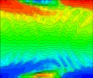


1. Introduction
Research in pulsatile flows was first considered in the context of arterial hemodynamics, later in pulmonary physiology and in engineering applications related to periodic flows in turbomachinery, and subsequently in other processes associated with transients and changes in operating conditions. Pulsatile flows have recently found renewed significance in their application to micro-electromechanical-systems-based microfluidic engineering applications that incorporate microscale pumping.
Womersley (Reference Womersley1955) provided the first exact solution of the Navier–Stokes equations of an oscillatory, incompressible flow in a circular pipe assuming a fully developed velocity profile, in which the ratio of the vorticity diffusion time scale,  ${R^2}/\nu $, over the time scale of the pulsation,
 $1/\omega $, was the governing parameter. Here, R is the radius of the pipe,
 $\nu $ is the kinematic viscosity and
 $\omega $ is the angular velocity of the pulsation. This parameter was the precursor of what was later adopted as the Womersley number,
 $Wo = \omega ({R^2}/\nu )$, which can also be defined as the ratio of the inertia forces,
 $\rho \omega U$, over the viscous forces,
 $\mu U/{R^2}$.
The receptivity of arterial blood flow in response to perturbations, which determines its stability and evolution can have significant implications for altered vascular wall shear stresses and overall vascular impedance (Ku Reference Ku1997). A classical steady pipe flow transition to turbulence, according to the road map of Morkovin (Reference Morkovin1985), is considered to be a bypass transition, which is a generic classification of processes occurring instantaneously emanating from non-modal energy growth mechanisms. Experimental results of Hof, Juel & Mullin (Reference Hof, Juel and Mullin2003) suggest that both non-modal energy growth and self-sustaining mechanisms could be important to understand the pipe flow transition. It appears that the physical mechanisms describing the transition are not very well accepted and discrepancies exist (see Eckhardt et al. Reference Eckhardt, Schneider, Hof and Westerweel2007; Avila et al. Reference Avila, Moxey, De Lozar, Avila, Barkley and Hof2011; Mullin Reference Mullin2011; Xu et al. Reference Xu, Warnecke, Song, Ma and Hof2017). At the centre of the disagreement is the long-puzzling, unphysical result that linear stability analyses lead to no transition in the pipe flow. The formation of puffs and slugs has also been reported, first by Wygnanski & Champagne (Reference Wygnanski and Champagne1973), to be a characteristic associated with a steady pipe flow transition, which appears to occur at a Reynolds number (Re) of  $Re \approx 2300$ in facilities with an average to low level of disturbances present in the flow set-up. When pulsation is applied, additional complexities are introduced into the flow field, which can reduce the critical
 $\; Re$ down to a mean
 $Re \approx 1500$ (Hershey & Im Reference Hershey and Im1968). However, the transition can be delayed to a much larger critical
 $Re$ in facilities with ultra-low disturbances. To avoid such variability in the critical
 $Re$, many researchers opted for a controlled perturbation of the flow by means of a ring-type turbulator placed upstream in the pipe which, according to Durst & Ünsal (Reference Durst and Ünsal2006), forces transition at a fixed critical mean
 $Re$.
Fedele, Hitt & Prabhu (Reference Fedele, Hitt and Prabhu2005) revisited the problem of the stability of a pulsatile pipe flow for axisymmetric perturbations by solving the Orr–Sommerfeld equation, by means of a Galerkin projection onto a function space spanned by a finite set of the eigenfunctions of the longwave-limit Orr–Sommerfeld operator. They found that flow structures giving the largest energy growth are toroidal vortex tubes.
Pulsatile flows are dominated by the interplay between inertia and shear forces. Near the wall, inertia appears to yield to the predominant shearing forces; however, away from the wall, inertia dominates where shear forces play a less critical role. Because breaking to turbulence is a spontaneous process that takes place globally, it starts very close to the wall and then subsequently propagates towards the centreline of the pipe as the  $Re$ increases beyond its critical value (Eckmann & Grotberg Reference Eckmann and Grotberg1991).
Turbulence is always enhanced during the adverse pressure gradient (APG) phase of the pulsation, where deceleration destabilizes the flow, and it is suppressed during the favourable pressure gradient (FPG) phase of the modulation when the flow is accelerated. This is the case for the phase-locked turbulence described by Stettler & Fazle Hussain (Reference Stettler and Fazle Hussain1986), who reported the existence of intermittent turbulent puffs that were also phase-locked. Puffs have also been observed by Trip et al. (Reference Trip, Kuik, Westerweel and Poelma2012) in the phase-locked regime of low amplitude pulsations having a duration of multiple periods and long physical length.
The effects of different waveforms of pulsation on the flow transition have been investigated by Brindise & Vlachos (Reference Brindise and Vlachos2018). Their results show that the waveform with a longer deceleration phase duration induced the earliest onset of transition, while the waveform with a longer acceleration period delayed the onset of transition. It is not clear if puffs were observed in this experimental work. These authors also demonstrated that the rate of acceleration and the duration of the deceleration phase affected the onset of transition.
A class of pulsatile flows, which has received little attention, is one that includes reverse flow and unsteady separation. The corresponding velocity profiles have inflection points, and hence become unstable at relatively low Reynolds numbers. The instability and transition to turbulence and its evolution in such flows are the primary focus of this study. The only previous work pertinent to the present research is that by Das & Arakeri (Reference Das and Arakeri1998), who introduced only one trapezoidal pulse to a pipe flow, which included an accelerating ramp, a constant velocity phase and a deceleration down to zero velocity. Their flow visualization indicated the formation of a helical vortex as a result of the reverse flow instability. Quasi-steady linear stability analysis was also carried out, which showed that the wavenumber corresponding to maximum growth does not change much during the instability even though the velocity profile does change substantially. Nayak & Das (Reference Nayak and Das2006), in their unpublished work, carried out three-dimensional (3-D) linear instability analysis with an inflectional velocity profile from the experiments of Das & Arakeri (Reference Das and Arakeri1998) as the input. It was shown that the profile is unstable for both axisymmetric and non-axisymmetric modes. The non-axisymmetric mode (n = 1) was observed to be the most unstable for this particular case. The 3-D instability showed the observed helical nature of the flow.
The present work will also reflect upon similarities with studies on unsteady wall boundary layer separation over flat surfaces or airfoils whose complexities are yet to be fully understood. For instance, Sears & Telionis (Reference Sears and Telionis1975) and Telionis (Reference Telionis1981) demonstrated that the vanishing of wall shear stress, a common criterion in boundary layer separation under steady conditions, does not have any special significance in unsteady flows. Unsteady separation occurs downstream of the zero-wall shear stress point where a thin region of reverse flow exists, before the flow erupts and breaks away with a sudden thickening followed by the formation of vortices.
One obvious question associated with the onset of flow reversals in pulsatile flow is under which combination of governing parameters does a dynamic separation occur. Further questions are as follows. How does  $Wo$ affect the transition? Is the transition always initiated during the beginning deceleration phase of the pulsation cycle that coincides with the maximum velocity? What is the spatio-temporal structure of the flow during the accelerating or decelerating phases of the cycle?
The remainder of the paper is organized as follows. Section 2 revisits and revises the analytical solutions of developing laminar pulsatile flow in pipes and establishes the range of flow parameters necessary to obtain a reverse flow. A description of the experimental set-up, particle image velocimetry (PIV) instrumentation and the techniques used is provided in § 3. Section 4 presents the data analysis and processing techniques. The results are presented in § 5 and the conclusions are summarized in § 6.
2. Theoretical background: the reverse flow regime
An analytical tool has been developed to provide information on the flow parameters needed to determine the bounds of the reverse flow regime and provide insights for the design of the experimental work. Such information on the reverse flow regime is not available in the literature. This tool simulates approximately the developing part of the flow generated by the motion of the piston which is initially at rest, as well as the fully developed flow stage which follows. The simulation is based on the assumption that the convection velocity,  ${U_0}$, which appears in the inertia terms of Navier–Stokes equations, remains unchanged throughout the entrance and fully developed regions. This assumption lifts the nonlinearity from the equations of motion and provides a way to analytical solutions with reasonable results. This approach, which was first applied to steady laminar flows near the entrance of a circular tube, has been attributed to Targ (see Slezkin Reference Slezkin1955). Since then, it has been applied to pulsatile flows (Atabek & Chang Reference Atabek and Chang1961; Yokota & Nakano Reference Yokota and Nakano1980). If the requirement of a developing flow is relaxed and replaced by the fully developed flow assumption, then the original solution by Womersley (Reference Womersley1955) is obtained.
It is appropriate to use the cylindrical coordinates  $r,\theta ,x$ in the present analysis, where the x-axis is aligned with the horizontal axis of the tube with the origin at its entrance. The flow is assumed to be axisymmetric, i.e. independent of
 $\theta $, and the equations expressing the momentum conservation in two directions and mass conservation are
 \begin{gather}\rho \left( {\frac{{\partial U}}{{\partial t}} + U\frac{{\partial U}}{{\partial x}} + V\frac{{\partial U}}{{\partial r}}} \right) ={-} \frac{{\textrm{d}p}}{{\textrm{d}x}} + \frac{{\partial {\tau _{xx}}}}{{\partial x}} + \frac{1}{r}\frac{{\partial r{\tau _{rx}}}}{{\partial r}},\end{gather}
 \begin{gather}\rho \left( {\frac{{\partial V}}{{\partial t}} + U\frac{{\partial V}}{{\partial x}} + V\frac{{\partial V}}{{\partial r}}} \right) ={-} \frac{{\textrm{d}p}}{{\textrm{d}r}} + \frac{{\partial {\tau _{xr}}}}{{\partial x}}\; + \; \frac{1}{r}\frac{{\partial r{\tau _{rr}}}}{{\partial r}},\end{gather}
 \begin{gather}\frac{{\partial U}}{{\partial x}} + \frac{1}{r}\frac{{\partial rV}}{{\partial r}} = 0,\end{gather}
The velocity distribution at the entrance of the pipe is assumed to be uniform and, therefore, will be a periodic function of time that may be provided in terms of the Fourier series as
 \begin{equation}U{(x,r,t)_{x = 0}} = {U_0} + \mathop \sum \limits_{k = 1}^n Re({u_{os,k}}\,{\textrm{e}^{\textrm{i}k\omega t}}),\end{equation}
where  ${U_o}$ is the time-averaged velocity and
 ${u_{os,k}}$ is a typical amplitude of the oscillatory velocity component of the pulsation. For simplicity, only one term of the Fourier series will be considered, i.e.
 \begin{equation}{u_f} = U{(x,r,t)_{x = 0}} = {U_0} + {u_{os}}\sin (\omega t).\end{equation}
Figure 1 depicts the definitions of  ${U_0}$ and
 ${u_{os}}$ in the context of a sinusoidal velocity modulation.
Definitions of  ${U_0}$ and
 ${u_{os}}$ in a typical sinusoidal velocity at
 $x/D = 0$.

According to Targ, the inertia terms are substituted by  $[{U_0} + {u_{os}}\sin (\omega t)](\partial U/\partial x)$.
It is further assumed that the radial velocity component V is negligible in general, and zero at the wall and centreline. Additionally, the stress gradients in the longitudinal direction are much smaller than the gradients in the radial direction and therefore can be ignored. Under these assumptions, the initial conditions, which agree with the experimental set-up and procedures, can be described as
 \begin{equation}{u_f}(0,r,t) = \left\{ {\begin{array}{*{20}{@{}ll@{}}} 0&{t \lt 0}\\ {{U_0} + {u_{os}}\sin (\omega t)}&{t \ge 0} \end{array}} \right\}.\end{equation}
Thus, the equation to solve is
 \begin{equation}\rho \left( {\frac{{\partial U}}{{\partial t}} + [{U_0} + {u_{os}}\sin (\omega t)]\frac{{\partial U}}{{\partial x}}} \right) = \rho \omega {u_{os}}\cos (\omega t) - \frac{2}{R}{\tau _w} + \frac{1}{r}\frac{{\partial r{\tau _{rx}}}}{{\partial r}}.\end{equation}
It appears that because of the initial conditions (2.6), the most convenient method to analytically solve the above equation is by using a Laplace transformation. Yokota & Nakano (Reference Yokota and Nakano1980) have provided such a solution for a developing pulsatile flow, which has been used to compute the velocity and shear stress profiles after some corrections and improvements.
The value of the shear stress at the wall,  ${\tau _w} = \tau (r = R)$, will be used to identify flow reversal events. The analytical solutions described above have been verified by using symbolic computations in Matlab and Mathematica. To validate the algorithmic implementation of the solution, several special cases were simulated. The first involves the development of the laminar flow without any oscillation at a fixed location x/D = 180, which corresponds to the position of the measured velocity field using PIV. This case is the result of an impulsive start of the flow from rest with
 $u = 0$ to
 ${U_0}$, according to the initial conditions in (2.6) applied at x/D = 0. Profiles of the velocity and shear stress at various times across half of the cross-section along the radius of the pipe at x/D = 180 are shown in figure 2. The graphs show the first instances after the initial conditions
 $u/{U_0} = 1$ and
 $u(r = R,x,t) = 0$ are enforced, which result in an initial zero-shear stress along with the radial distribution except very close to the wall, where it increases to high values at the subsequent time steps. As time advances, the velocity profiles change gradually from the plug-like initial profile to eventually reach a steady-state parabolic profile with maximum velocity
 $u/{U_0} = 2$. The stress distribution follows a similar pattern. It is transformed from initially non-existing stress throughout the flow field to a growing layer with substantial stress content near the wall, which eventually acquires a linear distribution across the maximum wall stress
 ${\tau _w} = 2$. This is in agreement with the classical fully developed laminar flow results.
Transient velocity and shear stress profiles obtained at x/D = 180 induced by the piston put in motion by a step change in velocity from 0 to  ${U_0}$ with
 ${u_{os}} = 0$. Curves are 2/3 s apart and arrows indicate increasing time. The value of angular velocity
 $\omega $ is arbitrarily set to
 $\omega = 2\mathrm{\pi}\,{\textrm{s}^{ - 1}}$.

A case of a typical pulsatile flow was also simulated analytically, in which the amplitude of pulsation was  $A = {u_{os}}/{U_0} = 1.0$. The instantaneous velocity and shear stress profiles, plotted in figure 3, clearly show a large flow region above
 $r/R \gt 0.62$ close to the wall with weakly-reverse flow patterns, based on the low values of the velocity and shear stress, and a rather strongly-reverse flow region above
 $r/R \gt 0.82$, based on the larger values of the negative velocity and positive stress.
Transient velocity and shear stress profiles obtained at x/D = 180 induced by the piston put in pulsatile motion by a step change in velocity from 0 to  ${U_0}$ with
 ${u_{os}}/{U_0} = 1.0$. Curves are 0.1 s apart. The value of angular frequency is
 $\omega = 2\mathrm{\pi }/T\; $ with
 $T = 1\;\textrm{s}$.

It is interesting to observe that the velocity at the centre of the pipe keeps increasing with time from its initial value of  $u/{U_0} = 1$ till it reaches its maximum value of 3, which corresponds to the fully developed state. One significant difference between the velocity patterns close to the wall and around the centreline is that the response time to reach the steady state is much shorter at locations closer to the wall than at points around the centreline.
The time-dependent stress changes sign with the frequency of pulsation and it appears that it spends a considerable amount of time being positive, i.e.  ${\tau _w} \gt 0$, which indicates the onset of reverse flow. From these analytical results, as well from our experimental conclusions, the wall is the first place that experiences changes in the flow structure, which subsequently propagate towards the centreline. For this reason, the wall has been chosen to identify the onset of reverse flow in the parametric investigation to establish the range of flow parameters that control it. The relative amount of time the flow spends in the reverse direction
 $I = T({\tau _w} \gt 0)/{T_{total}}$, defined as the reverse flow duration index (I), has been chosen to characterize the case quantitatively. A parametric study was carried out to quantify I for a range of values of the relative oscillatory amplitude
 ${A_1} = {u_{os}}/{U_0}$ and
 ${W_o}$. The results show a functional relation between
 $I,\; {A_1}$ and
 $Wo$. Regions with
 $I = 0$ are designated as no flow reversal regions and the blue line in figure 4 represents the best fit through the last points with
 $I \lt 0.001$. As the amplitude
 ${A_1}$ decreases to values less than 1, the no-reverse flow region is extended to higher
 ${W_o}$. If
 ${A_1} \gt 1$, then
 ${u_{os}} - {U_0} \gt 0$, and flow reversals appear right after the initial conditions are activated, regardless of the value of
 $Wo$. The most surprising result, however, is the narrow range of the two parameters,
 ${A_1}$ and
 $Wo$, required to not observe reverse flow.
Relation between pulsation amplitudes,  $A = {u_{os}}/{U_0}$, and pulsation frequencies,
 $Wo$, defining the boundaries between flow reversal and no-flow reversal regions.

Figure 4 demonstrates the boundary between the reverse flow and no-reverse flow regions on the relative pulsation amplitude and pulsation frequency plane. The graph also shows the values of the parameters chosen for the present experiments.
3. Experimental set-up
The experiments were carried out with the set-up shown in figure 5, in which water was used as a fluid medium. Pulsation was provided by the motion of a piston inside a cylindrical enclosure with a diameter of 140 mm and length of 910 mm. The piston was attached to a leadscrew, which was directly coupled to a programmable brushless DC servo motor, type Clearpath CPM-MCVC-3441-RLS manufactured by Teknic. The maximum speed of the motor was 850 rpm, which enabled a maximum piston velocity of 0.072 m s−1. At that speed, the water will be moving in the pipe at an average velocity of 3.87 m s−1 (average Re was 73500).
Experimental set-up with piston/cylinder to generate pulsatile flow undergoing transition to turbulence (not in scale).

The position of the piston was continuously recorded by a LASER proximity sensor, model Micro-Epsilon ILD1420-500. The red beam out of the semiconductor laser was aimed at a small, flat, smooth aluminium target plate mounted on the carriage of the lead screw. The distance was measured with an accuracy of 40 μm. The sampling rate was variable, with a maximum rate of 4 kHz (Δt = 0.25 ms), and the range of the measured linear distance was between 100 mm and 600 mm. To cover greater distances, the laser head had to be relocated. The digital output through an RS422 interface provided the measured distance as a function of time on a computer where the voltage of the pressure sensors was also recorded by analogue-to-digital converters. The processes on this computer and the PIV camera recordings on a second computer were triggered by an external pulse by the user. The distance, which was measured by the laser proximity sensor, was differentiated twice in time to obtain the velocity and acceleration of the piston, respectively.
Water flowed from the cylindrical plenum into an axisymmetric contraction, designed using a third-order polynomial fitted to the specified radius and length, and eventually, it entered a 3.65 m long rigid acrylic tube of 19 mm diameter. The test section was placed at x/D = 180 and it included an optical correction rectangular box filled with water and containing the pipe to mitigate optical distortions. The end of the tube was bifurcated to an 8 m long flexible acrylic pipe of 19 mm diameter returning the water to an open constant head reservoir. At the other end of the bifurcation, an attachment housing the calibration plate was mounted. The calibration plate was firmly connected to a thin long steel rod, which was able to slide all the way back to the test section through a small opening on the flange.
A secondary water circulating system could be reconfigured on the same set-up. This system used the constant head tank and a pump to drive the flow by appropriately opening the corresponding valves. This system extended the capabilities of the set-up to a Reynolds number of more than Re = 80 000. Data obtained in this configuration are not discussed in the present work.
Table 1 provides a list of the bulk flow parameters in the experiments, which includes the Reynolds number of the base flow,  $Re = \rho {U_o}D/\mu $; the Reynolds number of the pulsatile flow,
 $R{e_{os}} = \rho {u_{os}}D/\mu $; the relative amplitude of the pulsation,
 ${A_1} = \; {u_{os}}/{U_o}$; the Womersley number,
 ${W_o} = R{(\omega /\nu )^{1/2}}$; the Strouhal number,
 $Str = fD/({U_o} + {u_{os}})$; the Stokes number,
 $St = \omega {D^2}/\nu $; the Stokes layer thickness,
 ${\delta _{St}} = {(2\nu /\omega )^{1/2}}$; the Stokes Reynolds number,
 $Re{\delta _{St}} = {U_0}{\delta _{St}}/\nu$; and the flow frequency
 ${f_f} = {U_0}/D$. Here,
 ${W_o}$ and
 ${\delta _{St}}$ are related through
 ${W_o} = R{2^{1/2}}/{\delta _{St}}$.
Bulk flow parameters.

3.1. Particle image velocimetry techniques
Two-dimensional time-resolved particle image velocimetry (TR-PIV) techniques were used to acquire velocity data on the plane of laser illumination, which included the longitudinal axis of the acrylic pipe. The optical system consisted of a single-frequency continuous-wave Ar+ laser, model Spectra Physics Millennia Vs, which had a continuous output power of 5.5 W at 532 nm. The beam was reformed into a laser sheet using a cylindrical lens that illuminated a plane which bisected the flow field along the axis of symmetry. A fast frame-rate CMOS camera, Vision Research v710 Phantom, was used to acquire flow images with a 1200 × 800 pixel resolution. In each experiment, 20 000 images were acquired with a rate of 1 kHz. It should be mentioned that the present set-up was different from the usual PIV set-up, in which a YAG pulse laser is used in combination with a still camera. The water temperature was kept reasonably constant, within 0.5 °C, during the relatively short-time data acquisition. Hollow glass particles of 9–13 μm diameter (borosilicate glass spheres, LaVision 110P8) were used as tracers to visualize the flow. The PIV images were processed using an in-house modified code based on the open-source PIVLab software for Matlab platforms. This code is a multi-pass PIV algorithm using fast Fourier transform-based correlation. The initial interrogation size was 128 × 128 pixels, which was reduced to a final window size of 16 × 16 pixels during three iterations to improve the signal-to-noise ratio. A total of 82 × 41 vectors were generated per frame.
In the present case, the pipe radius was rather small,  $R = 9.525\;\textrm{mm}$, to achieve high longitudinal distances along the pipe,
 $x/D$, and therefore optical distortions were of concern. Such concerns were addressed by designing optical correction boxes, which contained water and the portion of the pipe where optical access was required. The design principle of these boxes was to minimize, where this was possible, the traveling time of the light through the various media.
Appropriate calibration targets were designed and fabricated by 3-D printing techniques, which were inserted in the pipe and used to enable spatial corrections in the post-processing phase of the data analysis. Although these corrective techniques can minimize image-distortion errors, additional improvements can be achieved by selecting optical media that have closely-matched refractive indices using an approach known as refractive index matching (RIM). This technique limits the physical processes of angular deviation of light during refraction and reflection at the interfaces between the optical media.
In the present work, we used two different pipe materials, acrylic and fluorinated ethylene propylene (FEP). The acrylic pipe was fabricated by using extrusion, which resulted in a greater optical uniformity. The FEP pipe was also produced by extrusion and it was tested here with two different wall thicknesses of 0.762 mm and 1.587 mm, and both had the same inner diameter. The thicker FEP material was more translucent and also revealed the non-isotropic passage of green laser light because of the density inhomogeneity of the material, most probably owing to the presence of layers generated by extrusion. Eventually, the thinner FEP material was adopted in the present investigation, although reasonable corrections to the optical distortions can be applied in the other case.
The uncertainty involved in the present PIV measurements depends on multiple sources of error such as the data processing algorithm, user inputs, flow characteristics and experimental set-up. The approach proposed by Charonko & Vlachos (Reference Charonko and Vlachos2013) has been adopted to provide estimates of the PIV measurement uncertainties. It is based on the primary peak ratio, Q, which represents the ratio between the primary peak in the correlation map and the second highest peak. It has been found by Charonko & Vlachos (Reference Charonko and Vlachos2013) that the uncertainty is inversely correlated to Q, regardless of the flow condition or image quality. Following the data in figure 7(a) of the referenced paper (2013), the indicative relative uncertainties have been estimated to be 0.15 % in the case of Re = 535 and 0.25 % in the case of Re = 4825. The reference value used is the corresponding velocity at the centreline.
3.2. Mass flow conservation
The flow generated by the linear motion of the piston entered the pipe directly without any losses with a rate of  ${\dot{m}_p}$. It is interesting to compare
 ${\dot{m}_p}$ with the mass flow rate obtained from the PIV measurements at a distance of
 $x/D = 183$,
 ${\dot{m}_{piv}}$, assuming the instantaneous flow velocity profiles are piece-wise invariant in the azimuthal direction. The piston displacement,
 ${L_p}(t)$, which was measured by the proximity laser, was differentiated with time to obtain the piston velocity
 ${W_p}(t) = \partial {L_p}(t)/\partial t$, which was used to compute the flow rate as a function of time
 ${\dot{m}_p}(t) = \rho {W_p}(t){A_p}$.
The measured velocity profiles on the vertical plane, x = 0, in cartesian coordinates, were integrated with the azimuthal direction  $\theta $ after reverting back to polar coordinates. The angle
 $\theta $ was measured from the y-axis of the Cartesian coordinate system, while r was always positive. The two velocity profiles in polar coordinates
 $u(x,\; r,\; \theta = 0,\; t)$ and
 $u(x,r,\theta = \mathrm{\pi },t)$ were integrated to provide
 \begin{align}{\dot{m}_{piv}}(t) = \rho \int_0^R {\int_{ - \mathrm{\pi }/2}^{\mathrm{\pi }/2} {u(x,\; r,\; \theta = 0,\; t)r\,\textrm{d}r\,\textrm{d}\theta } } + \rho \int_0^R {\int_{\mathrm{\pi }/2}^{ - \mathrm{\pi }/2} {u(x,r,\theta = \mathrm{\pi },t)r\,\textrm{d}r\,\textrm{d}\theta } } .\end{align}
The two time-dependent flow rates  ${\dot{m}_p}(t)$ and
 ${\dot{m}_{piv}}(t)$ for two of the four Reynolds numbers investigated here are plotted in figure 6, after normalization by the corresponding time-averaged value
 $\langle \dot{m}\rangle$. The two signals were highly correlated with a coefficient of cross correlation of 0.985 in the three low-Re cases and 0.966 in the case of Re = 4825. In these plots,
 ${\dot{m}_p}$ is a de-facto low-pass filtered signal, while
 ${\dot{m}_{piv}}$ is based on integrating the instantaneous signals of velocity. Considering the validity of the assumptions involved and the experimental uncertainty in the measurements, the agreement between the two estimates plotted in figure 6 was satisfactory. Most of the disagreement was in the moments of minimum flow rate where the assumption of the flow of azimuthal invariability breaks down owing to the developed asymmetry of the velocity profile. To provide some statistical information on the difference between the two flow rates, a time-dependent quantity was formed as
 $\Delta m(t) = {\dot{m}_p}(t) - {\dot{m}_{piv}}(t)$ and its time-averaged value was computed and compared with the time-averaged flowrate
 $\langle {\dot{m}_{piv}}\rangle $. Values of the ratio
 $\overline {\Delta m} /\langle {\dot{m}_{piv}}\rangle $ ranged from 0.023 in the three low-Re cases to 0.091 in the Re = 4825 case. The reason for this variability across the range of Reynolds numbers may be attributed to the assumption of piece-wise azimuthal invariability or, put another way, “quasi-axisymmetry” is only partially satisfied and the uncertainties in the measurements are higher, as evident in figure 6(b) where the flow rate
 ${\dot{m}_{piv}}(t)$ crosses the zero value for a short time at three instances. Overall, the two flow rates agreed reasonably well and conservation of mass was verified always within the assumptions made and uncertainties involved.
Comparison of mass flow rates obtained from piston displacement and PIV measurements at  $x/D = 183.75$. (a) Re = 535 and (b) Re = 4825.

Estimates of mass flow conservation at different x/D locations along the PIV measurement domain indicated a variability of 0.03–0.04 of the average  $\langle {\dot{m}_{piv}}\rangle $.
4. Data analysis: signal decomposition and reconstruction
The pulsation of the piston with a single frequency fp excites a number of frequencies in the flow inside the cylinder which are transmitted unchanged through the contracting nozzle into the pipe flow. Figure 7 shows two amplitude spectra of the longitudinal velocity fluctuations obtained at y/R = 0.93 and at y/R = 0.0, respectively, where the first three excited modes, fp, 2fp and 3fp, are marked and five additional modes up to 2 Hz are clearly visible but not marked. Very few low-amplitude fluctuations appeared to exist in the velocity spectrum at y/R = 0.0, which indicated that turbulence had not reached this location. On the contrary, moderate amplitude velocity fluctuations characterized the near-wall region.
Amplitude spectra of u-fluctuations obtained by PIV at a fixed x/D = 183.75, and y/R = 0.93 and y/R = 0.0 (centre line) in the case of Re = 1140. Piston pulsation frequency, fp = 0.25 Hz.

A closer look into the time-dependent signal at y/R = 0.93, at a fixed x/D = 183.75 location, is shown in figure 8, which indicated that the longitudinal velocity component was characterized by a low-frequency variation and higher-frequency components. These components could be attributed to turbulence and noise. This signal was a typical signal retrieved from the PIV data at a location close to the wall where the flow exhibits reversals. This figure shows signals of instantaneous velocity components, u and v, as well as longitudinal acceleration, a, as a function of time in the case of a flow with pulsation T = 4 s. The flow cycle appeared to contain one accelerating and one decelerating phase of T/2 duration followed by a period of T/2 where acceleration was insignificant. This behaviour was associated with the flow reversals and turbulence levels being low. It is evident that turbulence during the acceleration/deceleration phases was non-stationary here and a special treatment is required.
Low- and high-pass decomposition of u-fluctuations obtained by PIV at (x/D = 183.75, y/R = 0.93) in the case of Re = 1140. Piston pulsation frequency, fp= 0.25 Hz. Signals of  $u,{u_{LP}},\; {u_{HP}},\; {u_{rec}},\; v,\; a,\; TKE$ are displaced for visual aid.

The non-stationarity of turbulence data was addressed by using the trend removal method (TRM), which involved low-pass (LP) and high-pass (HP) filtering of the data, and by using empirical mode decomposition (EMD) together with the relevant Hilbert–Huang transform to determine the intrinsic mode functions (IMFs). This latter method, described in more detail in appendix A, is more appropriate for nonlinear and non-stationary cases for which traditional analysis involving classical Fourier decomposition is not directly applicable. Each of the two methods had its own advantages and disadvantages and the provided results complemented each other.
The time-dependent signals were mostly processed by applying TRM as in Xanthos, Gong & Andrepoulos (Reference Xanthos, Gong and Andrepoulos2007). The signals were decomposed into two major components, one with low-frequency content and one with high-frequency contributions by a LP and HP filtering of the signals. A typical quantity  $q(t)$, which involves velocity or vorticity components
 $u,v$ or
 $\omega $ can be decomposed as
 \begin{equation}q(t) = {q_{LP}}(t) + {q_{HP}}(t).\end{equation}
This decomposition can be considered as a direct outcome of the Fourier series expansion in-time of the original signal,  $q(t) = {q_0} + \sum\nolimits_{m = 1}^\infty {Re\{ {q_m}\,{\textrm{e}^{\textrm{i}m{\omega _p}t}}\} } $, where
 ${q_0}$ is the time-average of
 $q(t)$ (DC component),
 ${q_m}$ are the complex amplitudes and
 ${\omega _p} = 2\mathrm{\pi }{f_p}$ is the pulsating angular velocity. This decomposition rearranges the Fourier modes above and below a cut-off value
 ${\omega _c}$, so that
 \begin{equation}{q_{LP}}(t) = {q_o} + \mathop \sum \limits_{m = 1}^n Re\{ {q_m}\,{\textrm{e}^{\textrm{i}m{\omega _p}t}}\} \quad \textrm{for}\;m \le n,\end{equation}
and
 \begin{equation}{q_{HP}}(t) = \mathop \sum \limits_{m = n + 1}^\infty Re\{ {q_m}\,{\textrm{e}^{\textrm{i}m{\omega _p}t}}\} \quad \textrm{for}\;m \gt n,\end{equation}
where n is usually selected to be a multiple of the 1st harmonic, i.e. the pulsation frequency,  ${\omega _c} = n{\omega _p}$. In the present work, n was kept between 4 and 8, a range which was adequate in preserving the presence of discrete and visually identifiable frequencies in the
 ${q_{LP}}$ component that could represent instabilities like Kelvin–Helmholtz (K–H) instabilities. Although the process of selecting a cut-off frequency was not entirely objective, the effects of small variations of
 ${\omega _c}$ were not large on the relative fluctuations level,
 ${\sigma _{HP}}/{\sigma _{uref}}$.
The decomposition of the longitudinal velocity  $u(t)$ into its LP- and HP-filtered components,
 ${u_{LP}}(t)$ and
 ${u_{HP}}(t)$, respectively, where
 ${u_{HP}}(t)$ also contains the noise. is shown in figure 8. To demonstrate the effectiveness of the decomposition, the two components were re-combined to form the reconstructed signal
 \begin{equation}\; {u_{LP}}(t) + {u_{HP}}(t) = {u_{ref}}(t).\end{equation}
As is shown in this figure, the reconstructed signal did not differ from the original signal  $u(t)$. In fact, when superimposed on top of each other, they were identical. It should be also noted here that the signals of the
 $v(t)$ velocity component, shown also in the same figure, did not contain any obvious pulsatile characteristics. In addition, its mean flow was zero and therefore there was no need to apply this decomposition. The noise level was also low so that the actual
 $v(t)$ represents the turbulence fluctuations
 $v^{\prime}(t)$, i.e.
 $v(t) = v^{\prime}(t)$. If we define the turbulent kinetic energy (TKE) per unit mass, as the addition of the two kinetic energies of the two velocity components, where
 $TKE = 1/2({u^{\prime^2}} + {v^{\prime^2}})$, its intermittent behaviour can be also seen in figure 8. Turbulence is present in regions where the flow decelerates and is suppressed during accelerations of the flow. It appears that turbulence is relaminarized between the turbulence bursts.
Figure 9 shows the sensitivity of standard deviations of the LP and HP longitudinal-velocity components,  ${\sigma _{LP}}$ and
 ${\sigma _{HP}}$, respectively, which are normalized by the standard deviation of the original signal
 ${\sigma _{uref}}$ to changes in the cutoff frequency from 2 to
 $80{\omega _p}$. There is a linear variation of both quantities with
 ${\omega _c}$ for
 ${\omega _c} \gt 6{\omega _p}$;
 ${\sigma _{LP}}$ increases slightly, while
 ${\sigma _{HP}}$ decreases with a rate
 $(\partial {\sigma _{HP}}/\partial {\omega _c})({\omega _p}/{\sigma _{uref}})$ in the range of −2.4 × 10⁻³ to −3.0 × 10⁻⁴. This means that for a typical increase by 10 in
 ${\omega _c}/{\omega _p}$, the change in
 ${\sigma _{HP}}$ will be in the range
 ${\sigma _{HP}}/{\sigma _{uref}} ={-} 0.06$ to 0.0075, which is roughly 12 % to 5.0 % of the maximum value reduction.
Typical effects of frequency cut-off on  ${\sigma _{LP}}$ and
 ${\sigma _{HP}}$ in low- and high-pass decomposition on u- fluctuations obtained by PIV at x/D = 183.75 and y/R = 0.94, 0.89, 0.83, 0.78 and 0.73 in the case of Re = 1140. Piston pulsation frequency, fp= 0.25 Hz.

In practice, however, LP and HP filtering of the original signals is not simply the shifting of Fourier modes about  ${\omega _c}$ because this causes some distortion around the cut-off frequency, which is qualitatively the same for both filtering operations. The time scales of the pulsating low-frequency component and the time scales of turbulence were reasonably far apart from each other, and, therefore, no information was compromised by the data filtering. Low-pass filtering removed the fluctuations arising from turbulence from the signal so that the characteristics of the pulsatile motion were revealed as they were now separated from the turbulence. High-pass filtering removed the low-frequency effects of the flow and only turbulent fluctuations were retained with zero mean. This operation is called trend removal in signal processing (see Bendat & Piersol Reference Bendat and Piersol1980). The
 ${q_{HP}}(t)$ was further low-pass filtered at 60 Hz to eliminate the high-frequency noise shown in the spectra above, so that
 \begin{equation}{q_{HP}}(t) = q^{\prime}(t) + \Delta q(t),\end{equation}
where  $q^{\prime}(t)$ is the actual turbulence and
 $\Delta q(t)$ is the noise.
It should be noted that the present decomposition introduces additional complexities when it is applied to quantities raised to powers, the most common of which is  ${q^2}$. Such complexities involve shifting of the frequency content to twice the corresponding frequency in the original Fourier modes of q and cross modal interactions within the HP zone. Relation (4.1) for
 ${q^2}$ will be in the form of
 \begin{equation}{q^2}(t) = q_{LP}^2(t) + q_{HP}^2(t) + 2{q_{LP}}(t){q_{HP}}(t).\end{equation}
It is the last term  $2{q_{LP}}(t){q_{HP}}(t)$ that introduces mixed modes interactions across two different zones, i.e. LP and HP. The time-averaged values of
 $\langle {q_{HP}}(t)\rangle = 0$ and
 $\langle {q_{LP}}(t)\rangle = 0$ are obtained. If one compares this with a Reynolds decomposition
 \begin{equation}{u^2} = {(\bar{U} + u^{\prime})^2} = {\bar{U}^2} + {u^{\prime^2}} + 2\bar{U}u^{\prime},\end{equation}
the difference is obvious. Its time-average is provided by
 \begin{equation}\overline {{u^2}} = {\bar{U}^2} + \overline {{{u^{\prime}}^2}} ,\end{equation}
while the time average of (4.5) is
 \begin{equation}\sigma _{uref}^2 = \sigma _{LP}^2 + \sigma _{HP}^2 + 2\overline {{q_{LP}}{q_{HP}}} .\end{equation}
Each of the three terms on the right-hand side of this equation has to be computed from the measured velocity field, and  $\sigma _{LP}^2/\sigma _{uref}^2$,
 $\sigma _{HP}^2/\sigma _{uref}^2$,
 $2\overline {{q_{LP}}{q_{HP}}} /\sigma _{uref}^2$ are plotted in figure 10. The results show that the cross-correlation term,
 $2\overline {{q_{LP}}{q_{HP}}} $, at most has values close to 8 % at
 ${\omega _c} = 2{\omega _p}$ and usually the range of frequencies actually used is below 0.4 %. If this value is referenced to the value of
 $\sigma _{HP}^2/\sigma _{uref}^2$ at the corresponding
 ${\omega _c} = 8{\omega _p}$, it is 18 %. Thus, this term, which represents the nonlinear dynamics of the zones/components, may be small but it is not negligible. The graph also shows that the three fractions representing the three terms on the right-hand side of (4.7) add up to 1, as is expected, with reasonable accuracy everywhere except for the first two points.
Typical effects of frequency cut-off on  $\sigma _{LP}^2/\sigma _{uref}^2$,
 $\sigma _{HP}^2/\sigma _{uref}^2$ and
 $2\overline {{q_{LP}}{q_{HP}}} /\sigma _{uref}^2$ in low- and high-pass decomposition on u-fluctuations obtained by PIV at x/D = 183.75 and y/R = 0.94, 0.89, 0.83, 0.78 and 0.73 in the case of Re = 1140. Piston pulsation frequency, fp= 0.25 Hz.

5. Results
5.1. Phased-averaged structure
A more comprehensive and informative description of the underlying physical processes in the present flow involves a discussion of the phase-averaged results of  ${\omega _{z,LP}}R/\; {U_0}$ vorticity and
 ${u_{LP}}/\; {U_0}$ velocity plotted as shown in figures 11(a) and 11(b). The PIV data were processed first by low-pass filtering at 6 Hz and 10 Hz for the
 $Re = 535$ and
 $Re = 2285$ cases, respectively. These cut-off frequencies were selected to be lower than the range of turbulence so that the evolution of large-scale flow structures was captured. The cycle began and ended at the maximum velocity instance. The results of normalized vorticity, shown in figure 11(a), indicated a reasonable symmetry between the upper and lower walls. A large wall vortical layer (WVL) attached to the solid boundary was identified between
 $t/T = 0$ and 0.19. The WLV decelerated in this range at the end of which inflectional instability seemed to occur and it became separated at
 $t/T = 0.19$. On the high-velocity side of the WVL, four strips/fingers of vorticity protruded into the external flow which, most probably, were associated with K–H instabilities of the shear layer that formed vortical structures with an approximate frequency
 ${f_{KH}} \approx 8\;\textrm{to}\;10{f_p} = 2\;\textrm{to}\;2.5\;\textrm{Hz}$. It is interesting to observe that the maximum and minimum vorticity, mostly arising from the high values of the velocity gradient
 $\textrm{d}u/\textrm{d}y$, were found at
 $t/T = 0$. It is likely that this was the location where K–H instability was triggered.
(a) Normalized phase-averaged vorticity contours,  ${\omega _{z,LP}}R/\; {U_0}$. Cycle starts at maximum velocity. Case of Re = 535 with 0.25 Hz pulsation. Data obtained at x/D = 183.75. (b) Normalized phase-averaged velocity contours,
 ${u_{LP}}/\; {U_0}$, with superimposed iso-vorticity lines. Cycle starts at maximum velocity. Case of Re = 535 with 0.25 Hz pulsation. Data obtained at x/D = 183.75.

Between 0.19 and  $0.5t/T$, the separated shear layer was decelerating although with an increasing rate,
 ${\textrm{d}^2}u/\textrm{d}{t^2} \gt 0$. At
 $0.5t/T$, the velocity reached its minimum value and acceleration
 $\textrm{d}u/\textrm{d}t = 0$, after which the shear layer started to bend towards the wall. Subsequently, the flow started to accelerate and the separated shear layer began to break-up into several larger vortical patches. As these vortical patches travelled downstream, they appeared to interact, were weakened by losing some of their strength, or merged with the newly developing WLV. Obviously, these break away structures had their origin at the K–H vortices and now moved with a faster rate up to the second inflectional point after which, the rate of acceleration started to drop. Their orientation most probably was a result of the pressure gradient developing between the low pressure in the WVL and the higher pressure in the middle of the pipe. For a similar reason, the K–H vortices were inclined in a symmetrical way.
Another major feature of the present flow was the formation of a large secondary vortical structure. This vortical structure was induced by the separated shear layer immediately above, which carried an opposite rotation that created and controlled the reverse flow. There was a remarkable difference between the structures at the top and lower walls. The structure at the top consisted of three smaller vortices, while that at the lower wall was a single-piece structure. As will be shown later, at these two locations, the flow was turbulent although the  $Re = 535$ was low. However, this turbulence remained localized and never reached the middle of the pipe.
The variability in shape and strength among the breakaway structures of the separated WVL at times  $t/T \gt 0.6$ also suggested that the flow was turbulent. Although these structures were located closer to the centreline, they never escaped the near-wall region.
The phase-averaged velocity contours superimposed with iso-vorticity lines are shown in figure 11(b). The overall flow appeared to be reasonably symmetric about the pipe axis and across all phases, which included the large recirculating zone that extended from 0. 2 to  $0.62t/T$ with a maximum depth of
 $0.4R$.
The density of velocity contours at the four corners of the domain at  $t/T = 0$ and 1 indicated that the velocity gradient
 $\textrm{d}u/\textrm{d}y$ was at the maximum at these phases, as exhibited in the data of vorticity shown in figure 11(a).
An obvious question to ask is what is the extent of these phase-averaged structures in the azimuthal direction. Qualitatively, all structures are expected to exist at every location. The WVL with both parts, the attached and separated layers, is expected to go around the circumference uninterrupted. The induced secondary vortical layer close to the wall below the WVL is also expected to exist, but variations are likely. The K–H vortices are also expected to be formed in a similar way in the azimuthal directions, but their location and formation may be different. In general, quantitative variability in the circumferential direction is expected in all structures.
As the  $Re$ is increased to 2285, more K–H-type undulations with vortical content are formed, which gradually grow and transform into elongated strips/fingers that erupt and break away into the free stream region above the WVL as vortical patches (see figure 12a). More than ten K–H vortices were formed at the high-velocity edge of the WVL, which separated at
 $0.3t/T$ and remained attached for 70 % of the cycle. It appeared that these K–H vortical structures grew during decelerations, while the detached patches from the front tip of the separated shear layer remained strong under a flow acceleration. It is evident that the separated WVL induced the secondary vortical layer below with opposite vorticity, which now was shorter in duration and thinner in vertical depth than that at Re = 535. This is also shown in figure 12(b), where contours of the
 ${u_{LP}}/\; {U_0}$ are plotted. This plot demonstrated that the profiles at
 $Re = 2285$ showed a rather flat velocity profile in the regions around the centreline and away from the wall, while the profiles at
 $Re = 535$ followed a parabolic spatial distribution.
(a) Normalized phase-averaged vorticity contours,  ${\omega _{z,LP}}R/\; {U_0}$. Cycle starts at maximum velocity. Case of Re = 2285 with 0.25 Hz pulsation. Data obtained at x/D = 183.75. (b) Normalized phase-averaged velocity contours,
 ${u_{LP}}/\; {U_0}$, with superimposed iso-vorticity lines. Cycle starts at maximum velocity. Case of Re = 2285 with 0.25 Hz pulsation. Data obtained at x/D = 183.75.

5.2. Spatio-temporal evolution
Additional insights into the underlying physics of the present flow were obtained by considering the instantaneous values of the LP and HP components of vorticity and velocity across the pipe over several cycles of pulsation. Figure 13(a) shows contours of instantaneous vorticity,  ${\omega _{z,LP}}R/\; {U_0}$, over three consecutive cycles. Obviously, there was some variability from cycle to cycle as well as within each cycle between the upper and lower halves of the pipe, although significant qualitative similarities existed. An important similarity was the number of protruding vortical strips into the flow above the WVLs, which arose from K–H instabilities triggered at these locations. There were four K–H vortices before and four after the maximum velocity location, which defined the sign of acceleration. The front tip of the separated WVL was bent towards the wall in all cycles, which suggested the possible formation of a typical vortex with a wrapped-around shear layer undergoing K–H instabilities.
(a) Contours of instantaneous vorticity,  ${\omega _{z,LP}}R/\; {U_0}$. Cycle starts at maximum velocity. Case of Re = 535 with 0.25 Hz pulsation. Data obtained at x/D = 183.75. (b) Contours of instantaneous vorticity fluctuations,
 ${\omega _{z,HP}}R/\; {U_0}$. Cycle starts at maximum velocity. Case of Re = 535 with 0.25 Hz pulsation. Data obtained at x/D = 183.75.

It is also interesting to observe that the structure of the induced secondary wall vortical layer appeared to be more homogeneous, in terms of its vorticity content, than what was found in their phase-averaged structure, which indicated that these structures were vortices.
In general, there are great quantitative and qualitative similarities and sometimes overlapping information between the phase-averaged and instantaneous data, although there are also substantial differences among them. One such difference, for instance, is the frequency content of the two quantities. The averaging process in the phase-averaged results integrates the data over frequency/time and the outcome is smoother contours in the graphs than those in the instantaneous data, in which a higher-frequency content is displayed by the rough-edged contours shown in the plotted results.
Of interest is the information related to the generation of turbulent fluctuations and particularly vorticity fluctuations in this periodic flow field. Contours of  ${\omega _{z,HP}}R/\; {U_0}$ fluctuations for the case of
 $Re = 535$ are shown in figure 13(b). Careful examination of the data revealed that vorticity fluctuations appear in the form of dipoles, each carrying one positive and one negative pole. Their amplitude/strength and extent/size depend on their location. We classified them according to their position such as near the wall where the attached WVL and the secondary vortex are located or separated WVL. High-vorticity fluctuations were found within the attached WVL at the beginning/end of each cycle, where the flow decelerated, and at the upstream side of the secondary vortex, where the flow impinged on the wall by the circulation of the vortex. Away from the wall, the vorticity dipoles were located in the protruding fingers of the K–H vortices or between the break away vortical patches. These two sets of dipoles with intense vorticity had symmetric inclinations with the respect to the minimum velocity locations at
 $t/T = 0.5$, and one was developing under deceleration, where APG effects were strong, and the other during acceleration. It is the latter characteristic of enhanced fluctuations which breaks down the widely accepted norm that acceleration, i.e. FPG effects, suppresses turbulence.
Plots of velocity contours  ${u_{LP}}/\; {U_0}$ are shown in figure 14(a). Superimposed on these contours are several vorticity contours
 ${\omega _{z,LP}}R/\; {U_0}$ from figure 13(a) for a better visual aid. The most significant feature in these plots was the extent in space and time of the secondary vortical layer that was generating the reverse flow. Between two consecutive recirculating regions, there was a high-shear area within the WVL, which generated high vorticity as well as significant fluctuations of
 ${u_{HP}}/\; {U_0}$ velocity, as shown in figure 14(b). These fluctuations, like in the case of vorticity fluctuations, appeared to be higher in the attached WVL and the reattachment region of the secondary vortex. These fluctuations in the near-wall constituted the so-called turbulent spots, which grew during the deceleration phase of the flow where APG effects were strong and present throughout the whole flow field. This phase also included the reversing of the flow direction and the associated dynamic flow reattachment, which strongly suggested that inflectional instability occurred during this time when the shear was large, which led to a breakout to turbulence. During this phase, when the flow decelerated throughout the whole flow field, turbulence had not reached the centre of the pipe flow region and, therefore, it was confined in the near-wall region. The most significant result was that at these low Reynolds numbers, localized turbulence was present near to the wall region because of phenomena associated with flow reversals and separation. Fluctuations in the fingers and separated vortical structures were significantly smaller in amplitude but not negligible. Some of these fluctuations were associated with the flow deceleration part of the phase for reasons that are not known at this time.
(a) Contours of instantaneous velocity,  ${u_{LP}}/\; {U_0}$. Cycle starts at maximum velocity. Case of Re = 535 with 0.25 Hz pulsation. Data obtained at x/D = 183.75. (b) Contours of instantaneous velocity fluctuations,
 ${u_{HP}}/\; {U_0}$. Cycle starts at maximum velocity. Case of Re = 535 with 0.25 Hz pulsation. Data obtained at x/D = 183.75.

It is not clear if and how these localized spots of turbulence are related to the so-called puffs observed in the higher transitional  $Re$ flows of Trip et al. (Reference Trip, Kuik, Westerweel and Poelma2012). Stettler & Fazle Hussain (Reference Stettler and Fazle Hussain1986) did not observe puffs in pulsatile flows with flow parameters close to those used in this work. It should be emphasized here that no turbulence promoters, such as orifice plates or fluid injectors, were used in the present experiments to induce well-controlled disturbances that lead to the periodic appearance of puffs. It appears that in the present flow, flow reversals and dynamic separation were sufficient to trigger instability and bypass turbulence.
As the Re increased, turbulence broke-out globally in the near-wall zone and spilled-out into the undisturbed free stream region around the centreline of the pipe. This is clearly evident in figure 15(b), where the  $Re = 2285$ results of vorticity are plotted for three cycles having the maximum velocity of the first as the origin. These values were antisymmetric and, according to the coordinate system used, they should be negative in the lower wall and positive on the top wall during the acceleration phase of the cycle when the flow is always attached to the pipe wall. Substantial turbulent activities were present, not only in regions close to the pipe wall but also in the middle section of the pipe. Regions undergoing K–H instability were now extended towards the centreline of the pipe. These vortical structures appeared simultaneously at all wall-normal locations across the cross-section of the pipe, they possessed some of the characteristics of puffs found in steady-state pipe flows undergoing bypass transition and were amplified during decelerations.
(a) Contours of instantaneous vorticity,  ${\omega _{z,LP}}R/\; {U_0}$. Cycle starts at maximum velocity. Case of Re = 2285 with 0.25 Hz pulsation. Data obtained at x/D = 183.75. (b) Contours of instantaneous vorticity fluctuations,
 ${\omega _{z,HP}}R/\; {U_0}$. Cycle starts at maximum velocity. Case of Re = 2285 with 0.25 Hz pulsation. Data obtained at x/D = 183.75.

It was also interesting to observe some cycle-to-cycle variabilities in the higher- $Re$ cases. In the first cycle, these vortical structures across the pipe appeared to be formed during decelerations while the second cycle exhibited such structures through accelerations and decelerations. The existence of subharmonics in the present pulsatile flow suggested possible interactions among the cycles, which could explain this variability.
The fact that large values of opposite  ${\omega _{z,LP}}$ existed at the same time at the top and lower walls of the cross-section suggested the existence of large-scale structures with a high degree of correlation and almost no particular phase-shift between the top and bottom wall vorticity signals, which indicated that these were vortical rings, not helical structures. It has been observed, however, in three-dimensional instability analysis of pipe flows undergoing unsteadiness by one square pulse (see Nayak & Das Reference Nayak and Das2006) with an inflectional velocity profile, such flows are unstable for both axisymmetric and non-axisymmetric modes. The fact that all data in the present experiments indicated no substantial phase differences between the top and bottom vortical structures suggests that these structures may be the outcome of an axisymmetric or higher-order azimuthal mode instability. The attached WVL, which indicates a vortex-like structure, fits this scenario. However, it was clearly shown in the present work that the K–H instability plays a significant role in generating turbulence. Such evidence of shear layer instability with smaller vortices coexisting with the major roll-up WVL suggest that this is the most likely structure responsible for the bypass turbulence in the present flows. The part of the present experimental results related to the vortex-like WVL structure agrees with the stability analysis of Fedele et al. (Reference Fedele, Hitt and Prabhu2005). It should be also noted that although the azimuthal extent of these ring WVL-vortices has not been investigated in detail, the PIV measurements of a horizontal section of the pipe indicated similar results.
The LP- and HP-filtered data of the longitudinal velocity component in the case of Re = 2285 are shown in figures 16(a) and 16(b).
(a) Contours of instantaneous velocity,  ${u_{LP}}/\; {U_0}$. Cycle starts at maximum velocity. Case of Re = 2285 with 0.25 Hz pulsation. Data obtained at x/D = 183.75. (b) Contours of instantaneous velocity fluctuations,
 ${u_{HP}}/\; {U_0}$. Cycle starts at maximum velocity. Case of Re = 2285 with 0.25 Hz pulsation. Data obtained at x/D = 183.75.

Turbulence was spread out in the core of the pipe (figure 16b) and, as was mentioned earlier, it correlated well with the deceleration signal and its undulations arising from K–H instability throughout the cross-section. These undulations, which are not repeatable from one cycle to another, were also associated with localized acceleration/deceleration events that had an effect on enhancing or suppressing turbulence. These signals were indicative of the turbulence present in the flow and they could be further processed to characterize its structure. It should be mentioned here that the instantaneous fluctuations appeared in pairs of positive and negative parts because their mean value was zero and, therefore, to satisfy this condition, the positive values should counterbalance the negative values.
Although the presence of small vortices identified in the present flow, which is determined for the first time by direct measurements of vorticity, is similar to the vortices hypothesized to exist in puffs of steady flows (Wygnanski & Champagne Reference Wygnanski and Champagne1973), the structures observed here cannot be classified as puffs because they are modulated by the pulsation frequency and dominated by its relative amplitude. In addition, they do not possess several geometric characteristics, like the conical shape of the downstream tail of turbulence at the centreline and initial turbulence at the wall at the upstream side (Stettler & Fazle Hussain Reference Stettler and Fazle Hussain1986), and they seem to form at  $Re \gt 2000$. In the work by Trip et al. (Reference Trip, Kuik, Westerweel and Poelma2012), puffs were observed in steady and low-amplitude pulsating flows having a duration of multiple pulsation periods and a long physical length. A typical puff is over 20 diameters in length and, therefore, extends over multiple measurement volumes. It is interesting to consider why puffs have not been observed in the present experiments. Could the formations of such structures be influenced by the length of the measurement volume or length of pipe set-up? The formation of flow structures was not influenced by the length of the measurement volume because care was taken to avoid steps in matching the two different material pieces together. The length of the measurement volume was sufficient to detect the passage of puffs if they were formed, because the average forward-moving convective velocity of the flow,
 $2{U_0}$, was sufficiently large to bring the puffs into the measuring volume within the duration of the experiments. For instance, if the puffs were formed at 80 diameters, the traveling time to 183 diameters appeared to be between 34 s and 3.4 s for the low and high Re, respectively, which was much less than the total data acquisition time of 120 s during which they should have been detected.
Differences in the experimental procedures and set-up may also provide some explanation as to why puffs were not observed. The two components of the flow field, i.e. the steady state and the pulsation, were introduced concurrently in the present work. Because puffs are flow structures that form first in steady-state flows, it is very possible that they have never had a chance to be formed in the present case, while in experiments where a steady flow is introduced first, puffs can be formed before pulsation is added.
The long wavelength and duration of puffs suggest that the cause of their formation may be a beating phenomenon between two slightly different frequencies such as minor variations in the frequencies of gear pumps or flow circulating devices.
However, the most probable reason as to why puffs were not observed in the present experiments was the large amplitude of the oscillatory component  ${A_1} = 0.9$, which caused massive flow separation. The experiments by Trip et al. (Reference Trip, Kuik, Westerweel and Poelma2012) covered a range of
 ${A_1}$ between 0.07 and 0.74, with
 $Wo$ between 0 and 25. Although the specific information regarding the cases in which puffs were observed was not provided, the difference in the set-up parameters between the two datasets and the appearance of flow separation in our experiments was probably adequate to explain the formation or lack thereof of puffs.
Additional information on the spatial development of velocity and vorticity fields was obtained by observing the supplementary movies, which are available at https://doi.org/10.1017/jfm.2021.269, generated from the PIV data. Two typical movies are appended here for the  $Re = 535$ and 2285 cases. Each frame of the two movies contained plots of instantaneous iso-vorticity contours of
 ${\omega _z}R/{U_0}$ superimposed on velocity vectors measured on the illumination plane. Images of the key frames in these movies are presented and discussed below. Figures 17(a) and 17(b) show frames with contours of iso-vorticity for the case of
 $Re = 535$ obtained at different phase/times. The first frame at
 $t/T = 0.54$ shows the vorticity contours and velocity vectors immediately after the maximum velocity was reached, when the deceleration started. The flow appeared to be reasonably symmetric with layers of continuous vorticity close to the top and bottom walls, which suggested a local laminar flow pattern. At the edge of this WVL, a layer of intermittent vorticity was observed with patches of concentrated vorticity, which indicated the existence of some discrete vortices that, most probably, were the results of K–H instability on the edge of the WVL. The longitudinal velocity profiles appeared to be parabolic in this frame and they slowly decreased with time. As the flow continued to decelerate, patches of opposite vorticity appeared immediately close to the wall, which suggested the first appearance of flow reversals. This is demonstrated in figure 17(b), which corresponds to phase
 $t/T = 0.71$, as well as the available sequence of frames in the corresponding video with vorticity contours and velocity vectors. This reverse flow region grew with time while the magnitude of its vorticity increased. However, the vorticity distribution in this new layer was not uniform (see figure 17c), which suggested the onset instability and transition, and the formation of vortices. At the same time, at the interface between the forward- and backward-moving flow regimes, where the shear was higher, some spatial undulations appeared with a wavelength of approximately 0.20–
 $0.25R$, which were indicative of K–H instabilities at the lower part of the separated WVL. Thus the WVL was subjected to K–H instabilities on both sides, upper and lower. This caused the part of the shear layer with the flow moving forward to completely breakdown into irregularly shaped vortical patterns which are characteristic of turbulence. Very close to the top wall, the vorticity level of the counter layer in the reversed flow was approximately
 $- 3{U_0}/R$, while the vorticity at the forward flowing structures was approximately
 $3{U_0}/R$. This suggested a relative shear of approximately
 $6{U_0}/R$, which was sufficient for the local shear layer to sustain turbulence even at this Re.
(a,b) Spatial development of instantaneous vorticity field with superimposed velocity vectors obtained at fixed times of the pulsation cycle, Re = 535. (a)  $t/T = 0.54$ and (b)
 $t/T = 0.71$. (c) Zoomed view (right) of the counter layers of vorticity when reverse flow appears at the top wall at
 $t/T = 0.95$ for Re = 535.

It should be noted here that a pipe flow transition to turbulence, according to the road map of Morkovin (Reference Morkovin1985), is considered to be a bypass transition. The present data suggest that this was the case here even at this low Re because of the K–H instabilities in the shear layer formed between the forward and reverse flows in the near-wall region.
Another observation that can be made here is that the flow reversal took place in a rather non-violent way.
The Re = 2285 case represents a flow in which transitioning turbulent flow patches generated in the near-wall region break out into the pipe area around the centreline. Additional principal features of the flow will be demonstrated in a series of figures of pairs of velocity and vorticity contours at the same phase/time.
At  $t/T = 0.373$, shown in figure 18(a), the flow appeared to be symmetric with fewer turbulence spots outside the WVL, which appeared to be turbulent. At
 $t/T = 0.538$, the flow started to decelerate, and flow structures appeared to escape the wall region and travelled towards the middle section of the pipe. Vortical structures appeared outside the wall region carrying out vorticity from 4 to
 $- 7{U_0}/R$. At
 $t/T = 0.698$, shown in figure 18(b), the first spots of flow reversals were observed with velocity contours indicating substantial non-uniformities. A large vortical structure was observed at the top wall, which extended more than 0.7R into the centre of the pipe region. At
 $t/T = 0.810$, the flow at the top-wall layer was reversed while the lower-wall layer was in standstill mode. Vortical structures inclined by 15° to 20° were present at the top part of the flow with a length of approximately
 $1R$. The entire flow field was filled with vortical spots, which is a characteristic of turbulence. At
 $t/T = 0.865$, the flow decelerated further, and became more irregular throughout the domain and partially reversed at the lower wall, while the reverse flow was present everywhere at the top-wall layer. Long vortical structures appeared in the vorticity field and reverse flow of opposite vorticity was evident at the top-wall layer. The vortical structures emanated from the top wall were stronger than those that originated in the lower-wall layer with a vorticity content of
 $5{U_0}/R$ compared with
 $3{U_0}/R$. Thus, the moment the flow reversed was associated with strong vortical interactions. This was the most significant difference from the low-
 $Re$ cases, where the end of the flow reversal was a much less violent process.
(a) Evolution of instantaneous velocity and vorticity fields with superimposed velocity vectors obtained at fixed times of the pulsation cycle  $Re = 2285$. (b) Evolution of instantaneous velocity and vorticity fields with superimposed velocity vectors obtained at fixed times of the pulsation cycle Re = 2285.

The flow acceleration phase followed by deceleration, which corresponds to favourable and adverse pressure gradients, have been reported in the literature to impact transition and turbulence generation and suppression in very different ways. It has been reported, for instance, that APG effects are associated with flow separation in boundary layers and diffusers. The present results have also shown the presence of flow reversals in all the Reynolds numbers investigated here. It will be interesting to show how acceleration changes with  $Re$. A normalized acceleration was introduced to characterize the APG effects, which is defined as
 $a = (1/{U_0})({R^2}/\nu )(\partial U/\partial t)$. This parameter describes the ratio of the inertia forces per unit volume of the flow,
 $\rho (\partial U/\partial t)$, over typical viscous forces,
 ${\tau _w}/R\sim \mu ({U_0}/{R^2})$. Recall that
 $Wo$ also describes the ratio of typical inertia forces over typical viscous forces. However, at the end,
 $Wo$ is independent of velocity and it appears to be constant throughout the whole flow field. In contrast, the normalized acceleration, a, changes across the various flow-field regions and in-time. It is also apparent that this parameter is proportional to the pressure gradient.
Time-dependent values of this normalized acceleration were also computed from the present experimental data for each location of the PIV measurement grid. Signals of low-pass acceleration data  ${a_{LP}}$ are shown in figure 19. The lower-
 $Re$ data showed the highest amplitude of approximately 300, while the remaining three cases exhibited amplitudes between 150 and 200. If the flow were laminar, the acceleration, according to the theory, would have been
 $\omega {u_{os}}\textrm{cos(}\omega t\textrm{)}$, which, in the non-dimensional formulation, would be
 ${a_{lam}} = ({u_{os}}/{U_0})({R^2}/\nu )\omega \textrm{cos(}\omega t\textrm{)}$. Because the ratio
 ${u_{os}}/{U_0}$ was approximately the same in the four experiments carried out here with a value of 0.89 or 0.95,
 $\omega = 1.57\;\textrm{rad}\;{\textrm{s}^{ - 1}}$ and therefore the amplitude of the laminar flow acceleration appeared to be
 $({u_{os}}/{U_0})({R^2}/\nu ) \approx 130$, while the corresponding amplitudes in the data plotted in figure 19 showed values from 300 at the lowest
 $Re = 535$ followed by 200 at
 $Re = 1140$. At
 $Re = 2285$ and 4825, the corresponding amplitudes were 160 and 150, respectively, which were surprisingly closer to the theoretical laminar estimates. The reason why the lowest Reynolds numbers exhibited the highest measured amplitudes among the four cases investigated here appeared to arise from the wall viscous effects and the fluid displacement towards the centreline. As demonstrated in figures 11(b) and 12(b), the maximum value of the velocity
 $u/{U_0}$ around the centreline region of the pipe appeared to be approximately 3.0 at
 $Re = 535$, while the corresponding maximum value was only 2.5 at
 $Re = 2285$.
Normalized low-pass acceleration data,  ${a_{LP}}$, for each of the four experiments. Phase/time has been shifted to align signals.

5.3. Structure of turbulence and its conditional sampling
To obtain further insight into the structural characteristics of the predominant events, which are associated with the structure of turbulence, the time-dependent signals of all three quantities of velocity, shear stress and vorticity components were interrogated using conditional sampling techniques as a tool to identify the major characteristics and details of the structure of these events coined turbulent spots or bursts. In this context, the stationary HP data were further processed to determine quantitatively the behaviour of turbulence during each cycle, i.e. its enhancement when the flow decelerated and its suppression when the flow accelerated.
The conditional-sampling algorithm is similar in principle to that used by Andreopoulos & Bradshaw (Reference Andreopoulos and Bradshaw1980) and Andreopoulos (Reference Andreopoulos1985). The aim of the present analysis was to differentiate turbulence within intense events, like bursts, from the flow outside, which contained laminar flow durations, noise or low-level fluctuations of turbulence. Accordingly, the following definitions have been made for the intermittency factor
 \begin{equation}{I_q} = \left\{ {\begin{array}{*{20}{@{}ll}} 1&{\textrm{if}\;{q_i}(\boldsymbol{x},t) \gt {\theta_1}\;\textrm{or}/\textrm{and}\;\dfrac{{\partial {q_i}(\boldsymbol{x},t)}}{{\partial t}} \gt {\theta_2}}\\ 0&{\textrm{Otherwise}} \end{array},} \right.\end{equation}
where  ${q_i}(\boldsymbol{x},t)$ is the
 $i\textrm{th}$ component of the fluctuating quantity
 $q(\boldsymbol{x},t)$ with a zero time-averaged value at a location
 $\boldsymbol{x}$ of the spatio-temporal domain. The data sets
 ${I_{q1}}$ and
 ${I_{q2}}$, obtained from the different conditioning criteria based on level and derivative,
 ${\theta _1}$ and
 ${\theta _2}$, respectively, were merged through a union defined as
 \begin{equation}{I_q} = {I_{q1}} \cup {I_{q2}}\{ i:i \in {I_{q1}}\;\textrm{or}/\textrm{and}\;i \in {I_{q2}}\} .\end{equation}
The ensemble-standard deviation values of a set of m conditional realizations  $q(\boldsymbol{x},{t_i})$ defined as
 \begin{equation}\langle q(\boldsymbol{x})\rangle = {\left[ {\frac{1}{{m - 1}}\mathop \sum \limits_{i = 1}^m q{{(\boldsymbol{x},{t_i})}^2}} \right]^{1/2}},\end{equation}
were generated for the two conditions of relation (5.1), i.e. the burst of turbulence, mostly typical within the turbulent spots, designated as high-intensity turbulence (HT), and otherwise, designated as low-intensity turbulence (LT). Efficient data processing routines involving data index manipulation were written, which produced normalized root mean square (rms) values of  ${u_{HP}}$,
 ${v_{HP}}$ and
 ${\omega _{z,HP}}$ fluctuations from the PIV measurements.
Figure 20 shows instantaneous signals of velocity components, shear stress  $uv$, vorticity, acceleration and intermittency function
 ${I_u}$ for the case of low Re = 535. To monitor the introduction and level of disturbances, data were recorded from the onset of the piston motion. In these plots, one can observe the absence of spikes or other disturbances other than low-level noise at the beginning of the signals, which corresponded to the transitioning of the piston motion from its linear mode to the onset of the pulsation cycle. Immediately after, at the first peak of the pulsation, as shown in the signal
 $u/{U_0}$, and at this low
 $Re$, the first spot broke-out with an amplitude much larger than the noise level. Turbulent spots appeared to be formed in all cycles during the time of maximum velocity of the flow. In fact, it was interesting to follow their appearance, as they were formed immediately after the first relaxation of the maximum acceleration,
 $\partial a(\boldsymbol{x},t)/\partial t \lt 0$. They reached their maximum value at approximately the beginning of deceleration,
 $a(\boldsymbol{x},t) \lt 0$, followed by a phase of decreasing amplitude till the maximum value of acceleration. It appeared that the growth and decline of turbulence within the turbulent spots correlated more with the rate of change of acceleration,
 $\partial a(\boldsymbol{x},t)/\partial t$, rather than the acceleration itself,
 $a(\boldsymbol{x},t)$, at least for the present low-Re flow. Although similar correlations have been reported by Brindise & Vlachos (Reference Brindise and Vlachos2018), such a result was unexpected because the rate of change of acceleration,
 $\partial a(\boldsymbol{x},t)/\partial t = {\partial ^2}u(\boldsymbol{x},t)/\partial {t^2}$, does not appear in the transport equations of momentum and kinetic energy. The rate of change of acceleration defines the inflection points of the velocity and therefore its concavity. The inflection points are determined by
 ${\partial ^2}u(\boldsymbol{x},t)/\partial {t^2} = 0$ and coincide with the extrema of acceleration
 $a(\boldsymbol{x},t)$. Turbulence is enhanced between two inflection points with the concavity of the velocity upwards, i.e.
 $\partial a(\boldsymbol{x},t)/\partial t \lt 0$ and is suppressed when concavity is directed downwards
 $\partial a(\boldsymbol{x},t)/\partial t \gt 0$. The best way to relate this finding to and incorporate it into the understanding of physics is to consider the rate of change with time of all the terms in the momentum or any other transport equation. This can be obtained by differentiating with respect to time the momentum equation and considering the balance of each term. Thus, the rate of change of pressure and shear force gradients are balanced by the rate of change of the temporal and convective accelerations. Because all data obtained are time-dependent, interpretation of the results under this conditional sampling technique may be helpful. Significant shear stress and vorticity fluctuations were present within the spots. As shown previously in figure 13(b), the location of spots is related to the attached WVL, which is undergoing possible inflectional instability combined with K–H instability. These results at
 $Re = 535$, as well as the results of the
 $Re = 1140$ case, clearly demonstrated that transition can take place at levels much lower than
 $Re = 2200$, because of flow reversals, and that turbulence is phase-locked. Turbulent spots were identified rather easily by the conditioning algorithm, as evident from the corresponding intermittency signal shown in figure 20. There were parts of the
 ${I_u}$ signal outside the main turbulent spots, which were characterized by frequent on–off switching in low-level turbulence. These parts were activated by large derivatives of the criteria rather than level, particularly during the increasing flow acceleration phase.
Instantaneous normalized signals of  $u,{u_{HP}},{v_{HP}},{u_{HP}}{v_{HP}},{\omega _{z,HP}}$, intermittency
 ${I_u}$, and acceleration scaled by factors of 1, 5, 5, 100, 0.1, 0.5 and 50 respectively. Signals are displaced from each other by 1, 1.5, 2 or 2.5 units. Signals are obtained at
 $(x/D = 183.75,y/R = 0.923)$. Case of
 $Re = 535$ with 0.25 Hz pulsation. Subscript
 $HP$ has been dropped in the plots for simplicity.

It is interesting to compare these results with the results shown in figure 21, where the signals for the Re = 2285 case are plotted. It appears that the main body of the turbulence was formed at the locations with a relaxing rate of acceleration,  $\partial a(\boldsymbol{x},t)/\partial t \lt 0$, which were bounded by its zero crossings. Figure 21 shows approximately five complete cycles of data and, in almost all of them, the maximum values of turbulence occurred inside the negative acceleration phase. However, what is interesting here was the appearance of turbulence during accelerations, which was not observed in the lower-Re = 535 case described before or in the Re = 1140 case, which was not presented here. It should be mentioned that the current understanding is that transition starts at the core of the WVL, where vorticity is highest, at the beginning of deceleration after the maximum velocity is reached and turbulence breaks out (see figure 13b).
Instantaneous normalized signals of  $u,{u_{HP}},{v_{HP}},{u_{HP}}{v_{HP}},{\omega _{z,HP}}$, intermittency
 ${I_u}$, and acceleration scaled by factors of 1, 5, 5, 100, 0.1, 0.5 and 50, respectively. Signals are displaced from each other by 1, 1.5, 2 or 3 units. Signals are obtained at
 $(x/D = 183.75,\; \; y/R = 0.923)$. Case of
 $Re = 2285$ with 0.25 Hz pulsation. Subscript
 $HP$ has been dropped in the plots for simplicity.

The present  $Re = 2285$ data in figure 21 demonstrated for the first time that turbulence can also break out during the acceleration of the flow, as exhibited in the first and third complete and the last incomplete cycles shown in this figure at times 2 s, 10.2 s and 18.2 s, respectively. It was also interesting to observe that this break out occurred at the same velocity level of approximately
 $- 0.6{U_0}$ below the average velocity
 ${U_0}$, which corresponded to a
 $Re$, based on the critical instantaneous velocity, of
 $R{e_i} \approx 920$. As was mentioned earlier, these fluctuations were associated with the breakaway of the large-scale vortical structures at the tip of the separated WVL, which originated from the K–H instability.
Further observations of the signals suggested some kind of variability of turbulence intensity among the cycles, which broke down the classification of phase-locked turbulence in this  $Re\; $ case. This variability, most probably, denoted subharmonic interactions between the cycles because the fundamental periodic structure was two or more pulsation cycles. It should be also mentioned here that at closer locations to the wall, more well-formed turbulent spots were observed (see figure 23 below) between the maximum and minimum deceleration, which corresponded to the zero crossings of the instantaneous velocity during the destabilizing phase of the cycle.
By considering the results of the highest  $Re = 4825$ case investigated here, shown in figure 22, turbulence could appear on the accelerating phase of the cycle only and not during deceleration. This clearly contradicted the observational data that turbulence in pulsatile flows appears during decelerations. More interesting was the fact that turbulence broke out at the minimum velocity point when the acceleration started and the local instantaneous
 $Re$ was very low,
 $R{e_i} \approx 460$, which, as expected, was close to the difference between the mean and oscillatory
 $Re$. While the appearance of turbulence was observed during acceleration, it was not clear why in three out of the four cycles, there was no significant amount of turbulence during the destabilizing phase of deceleration. Similar findings were also reported by Stettler and Fazle Hussain (Reference Stettler and Fazle Hussain1986) in the case of
 ${A_1} = 0.8$ and
 $Wo = 10$, which are values of these parameters very close to those used in the present investigation.
Instantaneous normalized signals of  $u,{u_{HP}},{v_{HP}},{u_{HP}}{v_{HP}},{\omega _{z,HP}}$, intermittency
 ${I_u}$, and acceleration scaled by factors of 1, 5, 5, 100, 0.1, 0.5 and 50, respectively. Signals are displaced from the origin by 1, 1.5, 2 or 3 units. Signals are obtained at
 $(x/D = 183.75,\; y/R = 0.923)$. Case of
 $Re = 4825$ with 0.25 Hz pulsation. Subscript
 $HP$ has been dropped in the plots for simplicity.

It has been demonstrated here and in Brindise and Vlachos (Reference Brindise and Vlachos2018) that the evolution of turbulence with time within the spots and within the cycle in general, as it is depicted by using the quantity  $q(\boldsymbol{x},{t_i})$ (velocity, stress, vorticity) as a metric, depends on the acceleration rate with time,
 $\textrm{d}a(\boldsymbol{x},t)/\textrm{d}t$. A better metric and probably more appropriate for this purpose of determining the onset, duration and intensity of turbulence in the spots is the gradient of the longitudinal velocity, u, in the longitudinal direction,
 $\textrm{d}{u_{LP}}/\textrm{d}x$. This spatial gradient is more appropriate to use because it is included in the generation of turbulent stresses/kinetic energy term in the corresponding transport equation of
 ${u_i}{u_j}$, which, according to the phenomenological description of turbulence in tensor notation in general terms, is
 $P ={-} {u_i}{u_j}(\partial {U_i}/\partial {x_j})$. This is the originating term leading to the classical turbulent energy production and diffusion terms. In the present case, there are two terms related to the production of TKE,
 $- uv(\partial U/\partial y)$ and
 $- ({u^2} - {v^2})(\partial U/\partial x)$. It appears that the radial velocity, v, is extremely small, practically zero. Under these circumstances, the main term responsible for generating turbulence is
 $- {u^2}(\partial U/\partial x)$, which is of interest here where the gradient
 $\partial U/\partial x$ plays a dominant role.
This gradient is also plotted in figure 23, which, according to the present notation, is designated as  $\textrm{d}{u_{LP}}/\textrm{d}x$. It is obvious that it can determine the duration of the turbulent spots by its zero-crossings very well, while the peak in fluctuations corresponds to its maximum value. It is clear that when
 $\textrm{d}{u_{LP}}/\textrm{d}x \gt 0$, fluctuations are enhanced and when
 $\textrm{d}{u_{LP}}/\textrm{d}x \lt 0$, fluctuations are considerably reduced to small values, which seem to follow the above TKE production term. The difference in the outcomes of the two methods, i.e. one based on acceleration a and the second on
 $\textrm{d}{u_{LP}}/\textrm{d}x$, is only between 2 % and 9 % in the case of the signals shown in figure 23. Eventually, however, the method based on acceleration was adopted because it has been proven to be robust, while the method based on the spatial gradient appeared to be less consistent owing to the numerical noise and its low magnitude in the region around the centreline.
Instantaneous normalized signals of  ${u_{HP}},{v_{HP}},{u_{HP}}{v_{HP}}$ and
 ${\omega _{z,HP}}$, scaled by factors of 5, 5, 200 and 1, respectively. Signals are displaced from each other by 1, 1.5 or 2 units. Time-dependent acceleration and
 $\textrm{d}{u_{LP}}/\textrm{d}x$ are also shown on the top and scaled by factors of 50 and 2, respectively. Signals are obtained at (x/D = 183.75, y/R = 0.948). Case of Re = 2285 with 0.25 Hz pulsation. Subscript
 $HP$ has been dropped in the plots for simplicity.

5.4. Effects of frequency pulsation
One additional experiment was carried out in which the frequency of pulsation was increased to 1 Hz, the corresponding non-dimensional pulsation was  $Wo = 23.75$ and the
 $Re$ was kept at
 $Re = 535$. The results are shown in figure 24. Although the level of this pulsation was considered extreme for currently known biological and engineering applications, it was very intriguing to explore its variation. It appeared that there was no adequate relaxation time of turbulence in the cycle and therefore the flow was completely turbulent. The major common feature of the longitudinal velocity, shear stress and vorticity fluctuations was the presence of sharp spike-like excursions in the signals, which were indicative of large perturbations at the velocity maximum instances where the destabilization started. As the data show, during the phase of acceleration decrease, turbulence was enhanced till the minimum acceleration was reached where the fluctuations started to decrease continuously till the maximum deceleration approached. In that respect, the observed behaviour of turbulence here was associated with destabilization at the zero crossing of acceleration, i.e. the maximum velocity locations. Although this is the classic case of pulsatile flow transition, what is new here is that, at the end of each cycle, there was substantial turbulence, which did not have sufficient time to be quenched and was carried over to the next cycle even at this low-
 $Re$ case This brings into consideration the need to compare the time-scale of turbulence to dissipate into heat or the eddy turnover time,
 ${T_\varepsilon } = {q^2}/\varepsilon $, with the pulse duration time T. Typical estimates of these scales showed that
 $T \lt {T_\varepsilon }$ in the present case of T = 1 s and
 $T \gg {T_\varepsilon }$ in the case of T = 4 s.
Instantaneous normalized signals of  $u,{u_{HP}},{v_{HP}},{u_{HP}}{v_{HP}},{\omega _{z,HP}}$, intermittency
 ${I_u}$, and acceleration scaled by factors of 1, 5, 5, 100, 0.1, 0.5 and 50, respectively. Signals are displaced from the origin by 1, 1.5, 2 or 3 units. Signals are obtained at
 $(x/D = 183.75,y/R = 0.923)$. Case of
 $Re = 535$ with 1 Hz pulsation. Subscript
 $HP$ has been dropped in the plots for simplicity.

5.5. Conditional statistics of turbulence
Figure 25 shows the conditional results of the normalized standard deviation of u,  $v\; $ and
 ${\omega _z}\; $, obtained in each of the four different
 $Re$ flows investigated here across several locations of the pipe.
Normalized standard deviation values conditioned on turbulence level. (a) Case of  $Re = 535$ with 0.25 Hz pulsation; (b) Case of
 $Re = 1140$ with 0.25 Hz pulsation; (c) Case of
 $Re = 2285$ with 0.25 Hz pulsation; (d) Case of
 $Re = 4825$ with 0.25 Hz pulsation.

These normalized quantities represent the intensity of the corresponding fluctuations in the two zones characterized as HT and LT, respectively. The shape of the distributions in the two cases of  $Re = 535$ and 1140 indicated two regions of interest, one very close to the wall and the second around the centre of the tube. Turbulence never reached the latter region and therefore the turbulence intensities there were very low, roughly 0.002 for all quantities. This value was related to the noise level in the experiment. In the regions close to the pipe wall in the
 $Re = 535$ case, the intensity at the top wall inside and outside the turbulent spot was
 $\langle {u_{HT}}\rangle /{U_0} = 0.118$ and
 $\langle {u_{LT}}\rangle /{U_0} = 0.012$, respectively. This suggested that, between the spots, there was actually turbulence of a significant level of 1.2 %. Similar, qualitatively, was the behaviour close to the lower wall albeit with asymmetry with respect to the top wall. The level of radial velocity fluctuations
 $\langle {v_{HT}}\rangle /{U_0}$, as well as
 $\langle {v_{LT}}\rangle /{U_0}$, was low in comparison to the level of longitudinal fluctuations but was definitely higher than that of those in the middle of the pipe. A significant level of vorticity fluctuations was observed in the upper wall, where a values of
 $\langle {\omega _{HT}}\rangle R/{U_0} = 0.096$ was found inside the turbulent spot and 0.022 was outside. In the lower-wall region, the intensity of vorticity fluctuations inside the spots was only slightly higher than that outside.
At  $Re = 1140$, the distributions were qualitatively similar to those obtained at the lower-
 $Re$ case with some substantially different quantitative results. Intensities remained high inside the spots but increased outside in the region close to the wall. In the middle of the pipe region, all data collapsed to a value close to 0.0044, which was still very low but somehow higher than the corresponding value measured at
 $Re = 535$.
At higher  $Re$, substantial differences in the level of turbulence intensities at the centre region of the pipe took place as evident in the results plotted in figures 25(c) and 25(d). Turbulence from the near-wall region reached the middle section of the pipe where turbulent spots with high-intensity fluctuations were identified. The intensity of longitudinal fluctuations,
 $\langle {u_{HT}}\rangle /{U_0}$, increased from 0.004 in the low-
 $Re$ cases to 0.04 in the two high-
 $Re$ cases. More surprising was the increase of the radial velocity fluctuations, which are considered in the literature as always having low values and not affected by the pulsation. They exhibited a large increase to 0.03 and 0.02 at
 $Re = 2285$ and
 $Re = 4825$, respectively.
The effect of increasing the pulsation frequency/ $Wo$ on turbulence statistics at low
 $Re = 535$ is demonstrated in figure 26. Excessive turbulence was generated in the near-wall layer owing to the lack of complete relaxation of turbulence within each cycle, which spread out in the external flow near the pipe centre. The peak intensity
 $\langle {u_{HT}}\rangle /{U_0}$ inside the wall was approximately 10.4 % and the same quantity at the pipe centre, which was considered as free stream flow, was 1.4 %. The first value inside the wall boundary layer was not unusual, given the fact that the flow separated too. The value of the intensity at the centreline at this low
 $Re$, however, was very unusual. The present conclusion that increasing
 $Wo$ decreases the critical
 $Re$ is in agreement with the findings of Nerem & Seed (Reference Nerem and Seed1972) and Falsetti et al. (Reference Falsetti, Carroll, Swope and Chen1983). In fact, the study of Falsetti et al. provided the ratio of
 $Re/Wo \gt 200$ as a criterion for the onset of turbulence, which apparently is not applicable to the present case. The present results extend the influence of pulsation beyond the
 $Wo = 10$ range determined by Stettler & Fazle Hussain (Reference Stettler and Fazle Hussain1986), who advocated that the influence of pulsation is limited to a<10.
Normalized standard deviation values conditioned on turbulence level. Case of  $Re = 535$ with 1 Hz.

In figure 27, we present the intensities of  $\langle {u_{HT}}\rangle /{U_0}$ and
 $\langle {\omega _{HT}}R\rangle /{U_0}$ measured at the centreline of the pipe as a function of the mean
 $Re$ and we compare them to a single measurement by Trip et al. (Reference Trip, Kuik, Westerweel and Poelma2012) obtained with an amplitude ratio of 0.75 and
 $Wo = 25$, parameters which are closest to those used in the present studies. However, there were considerable differences between the present experiments on pulsatile flows involving flow reversals and those of Trip et al., which apparently may be reversing according to the theoretical analysis described earlier that classifies the parameters of the flow as a flow with reversals for the
 $Wo$ and amplitude ratio mentioned above. Nevertheless, because the data to compare were obtained at the same flow locations, i.e. the centreline, under similar flow parameters, such a comparison may be meaningful. Both studies showed that the onset of turbulence intensities increased with increasing
 $Re$. They also agreed on the level of turbulence intensities at the transitioning flows regime with
 $Re \gt 2285$. This agreement further strengthens the claims of our work. The minor difference between the present turbulence intensity and that of Trip et al. was attributed to the difference in the fluctuating amplitude between the two cases.
Centre line and near-wall turbulence intensities,  $\langle {u_{HT}}\rangle /{U_0}$ and
 $\langle \omega R\rangle /{U_0}$ various
 $Re$ and
 $Wo$.

The present results also supported the conclusion that the onset of transition is not related to the local  $Re$ based on the value of the instantaneous velocity or the oscillatory
 $R{e_{os}}$, as found by Trip et al. It was also interesting to see that the intensity of vorticity fluctuations,
 $\langle {\omega _{HT}}R\rangle /{U_0}$, followed a similar dependence on
 $Re$ as the velocity fluctuations
 $\langle {u_{HT}}\rangle /{U_0}$ at y/D = 0. Although the two cases of lower
 $Re$ of the present study indicated a low-turbulence level at the centre line, they cannot be classified as turbulence-free because transition occurred at the near wall region where phase-locked turbulence appeared even at these low Reynolds numbers.
In figure 27, we also plotted the data for velocity and vorticity fluctuations,  $\langle {u_{HT}}\rangle /{U_0}$ and
 $\langle {\omega _{HT}}R\rangle /{U_0}$, respectively, at y/R = 0.94 located inside the wall region. The classical turbulence intensity based on velocity decreased with increasing
 $Re$ at low Reynolds numbers and then a typical plateau was developed up to the last
 $Re$ investigated here. The intensity based on vorticity fluctuations seemed to increase consistently with
 $Re$. Increasing
 $Wo$ by quadrupling the frequency of pulsation had a minor effect on vorticity fluctuations in the near-wall region and a moderate reduction in velocity fluctuations.
The turbulence fluctuations data were also plotted against the non-dimensional maximum acceleration  $a = (1/{U_0})({R^2}/\nu )(\partial U/\partial t)$, as shown in figure 28. Because turbulence breaks at this moment with destabilizing effects following, this type of scaling may be proven to be more appropriate than
 $Re$. It appears that acceleration is inversely proportional to
 $Re$ because
 $a = (1/Re)({R^3}/{\nu ^2})(\partial U/\partial t)$. The intensities at the centreline
 $y/R = 0$ tended to decrease with increasing acceleration and they tended to increase in the region near the wall. These results suggest that there is a correlation between statistical quantities of turbulence and normalized maximum acceleration, which is a quantity containing the effects of pulsation. It is also known that the normalized acceleration is a controlling parameter in pulsatile flows. However, what is significant in the present results is that the normalized acceleration provides a consistent trend of how the near-wall statistical turbulence increases with it, while most of the observations of instantaneous turbulence have indicated a dependence on the rate of acceleration.
Rescaling centreline and near wall turbulence intensities,  $\langle {u_{HT}}\rangle /{U_0}$ and
 $\langle \omega R\rangle /{U_0}$ against maximum acceleration for two different
 $Wo$.

6. Conclusions
The focus of the present research study was the phenomena related to the transition to turbulence and relaminarization in pulsatile flows that involve flow reversals. An analytical model was developed to establish the relations between the non-dimensional frequency of pulsation and its amplitude, which can lead to flow reversals in parts of the cycle. The results show that there is a remarkably narrow domain on the amplitude,  ${u_{os}}/{U_0}$ and
 $Wo$ plane, where no reversals are expected. Based on this analysis, values of these two parameters were selected to be implemented in the experiments which involved flow reversals.
A new experimental facility was designed, constructed and tested to implement pulsation with variable frequencies and amplitudes by using a carefully designed cylinder/piston assembly. The piston was driven by a programable DC servo motor, which provided the pulsation characteristics in a water flow system.
An uncommon set-up of 2-D time-resolved PIV was implemented by using a continuous wave laser and a high-frame-rate digital camera to acquire data in a RIM set-up of the optical correction box. This set-up provided spatio-temporal velocity data at fixed rates. Four different experiments were performed at  $Re = 535$, 1140, 2285, 4825 and
 $Wo = 11.91$, as well as one additional experiment at
 $Wo = 23.82$ and
 $Re = 535$.
The non-stationarity of turbulence data was addressed by using trend removal methods involving LP and HP filtering of the data, and by using EMD together with the relevant Hilbert–Huang transform to determine the IMFs. This latter method is more appropriate for nonlinear and non-stationary cases for which traditional analysis involving classical Fourier decomposition is not directly applicable. The EMD data analysis revealed the existence of several subharmonics in the vorticity and velocity fields, while the trend removal method indicated nonlinear dynamics though mixed-mode interactions between low and high frequencies. In addition, it was shown that the high-frequency components, which contain turbulence, have r.m.s. values lower than the low-frequency components that have a frequency content closer to the pulsation frequency  ${f_p}$.
The availability of time-dependent data of velocity and vorticity provided information related to the physics of changing direction in the near-wall region where flow reversals are evident. It appears that this process is gradual in the cases of the lowest  $Re$. During the end of the acceleration phase for low
 $Re$ or at the beginning of it for higher
 $Re$, vortical patches breakaway from the tip of the separated WVL, while the near-wall reversed flow has changed direction by crossing the zero level through a simple full stop. Confined turbulence in the near-wall region is observed at low
 $Re = 535$ and 1140. At higher
 $Re$, the entire flow field is filled with vortical spots characteristic of turbulence as the flow decelerates further and becomes more irregular through the whole domain, while flow reversals are more violent owing to strong vortical interactions. This is one difference between this
 $Re$ case and those at lower
 $Re$.
During the deceleration phase of the pulsation cycle, asymmetries start to develop between the top- and lower-wall regions. These asymmetries are reduced when the flow accelerates.
It was found that transition to turbulence is a spontaneous event covering the whole near-wall region. The instantaneous vorticity profiles suggest the development of a large-scale ring-like cylindrical attached wall vortical layer, which does not possess the characteristics of a toroidal vortex, on which smaller vortices of higher frequencies than the pulsation frequency are superimposed, which point to a K–H shear layer type of instability leading to the formation of smaller vortices on top of the major WVL structure. Inflectional instability causes the WVL to separate, which forms a toroidal vortex-like structure that is associated with the induction of a secondary vortical structure below it. The K–H vortices, located on both sides of the separated WVL, grow in size and start breaking away into smaller turbulence patches with vortical content in the longitudinal direction at low  $Re$ and in the radial at high
 $Re$. This appears to be the prevailing structure of the flow in each of the investigated Reynolds numbers. At high Reynolds numbers, the strength and extent of the vortices are larger and substantial disturbances appear in the free stream region of the flow, which are typical of pipe flows at transitional Reynolds numbers. It appears that the basic mechanism here is inflectional instability of attached WVL leading to a roll-up of the separated shear layer with the K–H vortices.
Turbulence appears to be produced at the locations of maximum or minimum vorticity within the attached WVL where deceleration starts, in the ridges between the K–H vortices around the separated WVL during acceleration and deceleration, and the upstream side of the secondary vortex where the flow impinges on the wall where rapid changes of streamline curvature occur that serve as a rapid inducer of turbulence. The near-wall turbulence breaks away into the middle pipe region through the eruptions of K–H vortices for  $Re\; \ge 2200$ under either deceleration or acceleration of the flow.
Although the presence of small vortices, which are identified in the present flow for the first time by direct measurements of vorticity, is similar to the vortices hypothesized to exist in puffs of steady flows, the structures observed here cannot be classified as puffs because they are modulated by the pulsation frequency and dominated by its relative amplitude. In addition, they do not possess several geometric characteristics like the conical shape of the downstream tail of turbulence at the centreline and initial turbulence at the wall on the upstream side.
The stationary HP data have been further processed to determine quantitively the behaviour of turbulence during each cycle by conditionally carrying out sampling analysis. It appears that the growth or decline of turbulence within the turbulent spots depends on the location within the flow domain and correlates more with the rate of change of acceleration,  $\partial a(\boldsymbol{x},t)/\partial t$, rather than the acceleration itself,
 $a(\boldsymbol{x},t)$. Time-averaged statistics, however, correlate better with the normalized acceleration
 ${a_{max}}(x)$.
These results for the  $Re = 535$ and
 $Re = 1140$ cases, clearly demonstrate that a transition can take place at much lower than
 $Re = 2200$, because of flow reversals, and that turbulence is phase-locked.
The effect of increasing the frequency of pulsation from 0.25 to 1 Hz, was also investigated at  $Re = 535$. It appears that there is no adequate relaxation time of the turbulence in the cycle and, therefore, the flow remains completely turbulent. As the data show, during the phase of acceleration decrease, turbulence is enhanced till the minimum acceleration is reached where the fluctuations start to decrease continuously till the maximum deceleration is approached. In that respect, the observed behaviour of turbulence here is associated with destabilization at the zero crossing of acceleration, i.e. the maximum velocity locations.
Supplementary movies
Supplementary movies are available at https://doi.org/10.1017/jfm.2021.269.
Funding
The financial support provided by NSF through grant CBET 1803845 and monitored by Dr R. Joslin is greatly appreciated.
Declaration of interests
The authors report no conflict of interest.
Appendix A. Intrinsic mode functions
As was mentioned earlier, the present data appeared to be non-stationary and, of course, nonlinear for which traditional analysis involving classical Fourier decomposition is not directly applicable.
Empirical mode decomposition (EMD) and the Hilbert–Huang transform (HHT) are also employed to process the present PIV data. The EMD (Huang et al. Reference Huang, Shen, Long and Liu1998; Huang, Shen & Long Reference Huang, Shen and Long1999; Wu & Huang Reference Wu and Huang2009) is an adaptive method introduced to analyse nonlinear and non-stationary signals. It provides a decomposition of the signals in fast and slow oscillations with frequency-dependent amplitude. A typical signal q(t) is decomposed as
 \begin{equation}q(t) = \mathop \sum \limits_{j = 1}^m {\psi _j}(t) + {r_m},\end{equation}
where  ${\psi _j}(t)$ is the intrinsic mode function (IMF) and
 ${r_m}$ is the residual of
 $q(t)$. Each
 ${\psi _j}(t)$erm is an IMF (see Huang et al. Reference Huang, Shen and Long1999), which can be represented in the form
 ${\psi _j}(t) = {r_j}(t)\cos {\theta _j}(t)$ where both the amplitude and phase are time dependent. The most common procedure to determine a polar representation of
 ${\psi _j}(t)\; $ is the Hilbert transform (HT).
In the present work, the ensemble empirical mode decomposition (EEMD), as presented by Wu & Huang (Reference Wu and Huang2009), has been applied to reveal any hidden intrinsic non-stationary oscillatory structures in a time series without undue mode mixing.
Figure 29 shows the IMFs obtained after applying EEMD to the signals of the u component at r/R = 0.93. The 1st intrinsic mode is an oscillation containing high frequencies while the 7th mode is an oscillation having the lowest frequency content. The original signal is recovered after adding all the modes. The signals are decomposed in the time domain and the length of the IMFs is the same as the original signal. These modes have been further processed by using the HHT, which preserves the characteristics of the varying frequency. This is an important advantage of HHT because a real-world signal usually has multiple causes happening at different time intervals. The HHT involves differentiation with the time of the EMDs and the imaginary part of HHT to obtain the angular velocity/frequency as a function of time, which does not always produce a smooth result particularly at the beginning and end of each of the modes.
Ensemble empirical mode decomposition with computed intrinsic mode functions of u-component signal at (x/D = 183.75, y/R = 0.93). Components 1 to 7 are displaced by multiples of 0.3 and multiplied by 15. Case of Re = 1140,  ${f_p} = 0.25\;\textrm{Hz}$.

The low-frequency modes are not entirely affected by this, but the higher modes exhibit some fluctuations because of this. The frequency variation in the low-frequency modes is rather small. At high-frequency modes, however, there is a substantial variation of frequency with time. Another interesting behaviour of the high-frequency modes is the appearance of bursting periodic structures with the duration of the pulsation time  ${T_p} = 1/{f_p}$. The frequency of appearance of these bursts suggests that this can be a signature of the bursts. This is shown in figure 30 where the 3rd IMF of the u-component is plotted, which is obtained at
 $r/R = 0.93$. The frequency content of these IMFs is between 2 and 8 Hz. It is also interesting to note that the 6th IMF, shown in figure 31, exhibits the main frequency of pulsation
 ${f_p} = 0.25\;\textrm{Hz}$, with minor variation, while the 7th IMF, plotted in figure 32, indicates a sub-harmonic of the pulsation frequency of approximately
 ${f_p}/2$. The most significant conclusion from this EMD analysis is the existence of multiple subharmonics in all
 $Re$ cases investigated here.
Third intrinsic mode functions of u-component signal at r/R = 0.93 and corresponding frequency variation with time obtained from Hilbert–Huang transform. Case of Re = 1140,  ${f_p} = 0.25\;\textrm{Hz}$.

Sixth intrinsic mode functions of u-component signal at r/R = 0.93 and corresponding frequency variation with time obtained from Hilbert–Huang Transform. Case of Re = 1140,  ${f_p} = 0.25\;\textrm{Hz}$.

Seventh intrinsic mode functions of u-component signal at r/R = 0.93 and corresponding frequency variation with time obtained from Hilbert–Huang transform. Case of Re = 1140,  ${f_p} = 0.25\;\textrm{Hz}$.



