Costanza and Finkelstein (Reference Costanza and Finkelstein2015) have justly argued that cross-sectional operationalizations of generational groups represent a confound that constrains the ability to unequivocally separate the effects of age and period. A related statistical argument against this practice bears consideration as well. Namely, cross-sectional operationalizations of generations have the potential to unduly inflate type two-error rates when compared with the analysis of simple age effects. This is a problem because true age effects can be erroneously ignored in studies where age is artificially split into assumed generational groups. Indeed, the argument against artificially bifurcating continuous data is not new (e.g., Cohen, Reference Cohen1983), however past attempts to make inferences about generational effects in cross-sectional designs present an opportunity to investigate the particularly insidious nature of this practice and its implications. To demonstrate the problem at hand, let us consider a brief empirical example by virtue of a simulation study.

To begin, let us design a hypothetical cross-sectional study to detect a hypothesized small- to moderate-sized positive bivariate correlation between chronological age (i.e., a continuous variable) and some continuous outcome of interest (Cohen, Reference Cohen1988). For the purposes of this example, the exact nature of the outcome is unimportant, as the focus here is on the operationalization of age. To test our hypothesis regarding this correlation, we randomly sample 150 participants from a population with a known mean age of μ = 40 (σ = 10.50). Assume that we have collected data regarding each participant's chronological age along with some scale indexing their level on our outcome of interest. In this scenario, we can also assume that the known population mean of this outcome is μ = 5 (σ = 1.25); however, this detail is less important than the bivariate relationship between age and our outcome. That said, let us also assume that the correlation between age and our outcome is ρ = .20. Note that this correlation is fixed by the population parameter. Thus, in our sample, observed differences between the known parameter and the estimated parameter are assumed to be caused by sampling error alone (i.e., remember, we are only sampling 150 participants in this study). Given this, when we look at the data, we observe a bivariate correlation between age and our outcome of r = .19, which is statistically significant, t(148) = 2.47, p = .01.

Next, we can separate our age variable into three distinct age categories to get a sense of whether or not there are “generational” effects at play. To accomplish this, we split our age variable into three equal groupings of N = 50 each (e.g., younger, middle-aged, older; however, this distinction is less important than the implications of the splitting procedure, as we will see). We then observe the correlation between our new categorical age variable and our outcome, r = .13, which is not statistically significant by conventional standards, t(148) = 1.64, at p = .10. There is a very good reason for this, in that meaningful variance is lost in the translation of continuous chronological age into age groups, which is occluding the ability to detect an effect (Cohen, Reference Cohen1983).

However, perhaps a bigger problem here is that there is a seemingly unlimited number of random samples of 150 participants that could be drawn from this population (i.e., if we assume that the population is infinite). Although each of these random samples would exhibit the same mean age (i.e., M = 40, SD = 10.50), the distribution of age in each is likely to vary from sample to sample. When we start artificially splitting such samples into age categories, we do so differently for each sample by virtue of the fact that each sample has a different age distribution. This is a problem because how you “cut” the data in such cases has the potential to greatly impact the inferences that you would make regarding the resulting categorical variable.

To illustrate this, a simulation study was conducted to replicate 1,000 hypothetical studies using the same methodology described above.Footnote ¹ Essentially, this involved randomly sampling 150 participants from our assumed population 1,000 times, cutting the resulting data into three distinct age groups using the same procedure and then observing the relationship between this new categorical age variable and the outcome. To demonstrate the problem at hand, we will consider three relevant parameters derived from simple linear models regressing our outcome onto this age category variable (i.e., variance explained—R ², standardized regression coefficients—β, and p-values representing the null-hypothesis significance test for the age group parameter).

These model parameters can be compared with the same parameters derived from a linear model with chronological age as a predictor. This is an important comparison because the chronological age–outcome relationship has been held constant in each of these simulated studies by virtue of the design of the simulation (i.e., the population parameter for the age–outcome relationship was specified a priori to ρ = .20, thus although the age distribution may change from sample to sample, the rank ordering of age and the outcome remains the same).

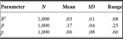
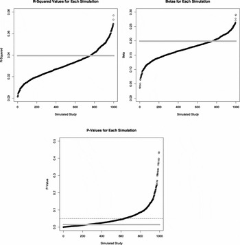
Table 1 presents descriptive statistics for these parameter estimates across the 1,000 simulated studies. Compared with known effects of chronological age (i.e., R ² = .04, β = .20, p = .01), on average, R ² and β are lower in categorical age models, whereas p-values are higher in categorical age models. To better understand the implications of these findings, each of these parameters were plotted across all 1,000 simulated studies (see Figure 1). Indeed, considering these representations, it is clear that there is quite a bit of variability in the observed parameters across all simulations.

Table 1.

Descriptive Statistics for Categorical Age Model Parameters From Simulation Study

Note. For comparison, chronological age parameters are as follows: R ² = .04, β = .20, and p = .01.

Figure 1.

Plots of categorical age model parameters versus continuous age model parameters from simulation study. In each plot, the grey line represents the value of the continuous age parameters, whereas the black line represents categorical age parameters. For p-values, the dashed line indicates conventional p < .05 cutoff.

More importantly, the actual rate of rejecting the null hypothesis of a categorical age effect in the presence of a chronological age effect can be determined. Indeed, for each sample, there is a known statistically significant effect of chronological age on the outcome. Thus, any difference in the conclusions drawn regarding the categorical age variable reflects an incorrect conclusion with respect to the true effect of chronological age. Moreover, because other factors were held constant (e.g., population mean and standard deviation of the assumed outcome), such differences could only occur by virtue of the way in which the chronological age variable was “cut” to form the categorical age variable. In this case, 368 out of 1,000 observed effects of categorical age were deemed to be not statistically significant from zero at p < .05. Essentially reflecting an assessment of statistical power, when considering categorical age, one would have incorrectly failed to reject the null hypothesis of an age effect 36.80% of the time. Keep in mind that this estimate is likely conservative, as these parameters resulted from randomly sampling from an assumed and known population. In reality, such studies are very unlikely to comprise truly representative samples, which would very likely exacerbate this effect.

Clearly there are myriad issues associated with cross-sectional representations of generational groups formed on the basis on chronological age. One problem with ascertaining whether or not there is a “there there” with respect to generational differences may stem from the fact that investigations that adopt cross-sectional methodologies for studying these effects are likely ignoring or at least obfuscating true effects of age. Although the substantive value of age effects can be questioned, it is reasonable to suggest that ignoring the possibility of valid inferences is ill advisable in the vast majority of instances. Thus, given the phenomena demonstrated here, I would argue that the cross-sectional operationalization of generations represents little more than an exercise in silliness.