

1. Introduction
The global adoption and commercialization of genetically modified organisms (GMOs) is occurring at a rapid pace. Global land planted with GMO crops increased from 1.7 million hectares in 1996 (the first year of adoption) to 179.7 million hectares in 2015. These plants have a novel combination of genetic material obtained using biotechnology. The crops that comprise the largest shares of the GMOs industry are soybeans, maize, and cotton. As of 2015, the shares of global land area planted with GMO soybeans, maize, and cotton were 83%, 29%, and 75%, respectively (James, Reference James2014, Reference James2015). The global land area dedicated to non-GMO varieties is decreasing rapidily for these crops.
Country adoption of GMO crops varies widely. Commercialization of GMO crops began in the US and Canada, but has spread worldwide. In 2015, approximately 54% of global land area allocated to GMO crops was in industrialized countries and 46% in developing countries. Countries with more than 10 million hectares of GMO crops include the US, Brazil, Argentina, India, and Canada (James, Reference James2015). Countries experiencing rapid growth in GMO crops include China, Paraguay, Pakistan, South Africa, Uruguay, and Bolivia. Countries that have resisted the development, adoption, and import of GMOs include the EU, Japan, and developing countries who export to non-GMO countries.
Policies for regulating GMOs vary widely across countries. National policies include regulations related to the approval process, risk assessment, labeling, traceability and identity preservation, and coexistence of GMO and traditional crops. Countries also differ in membership to international treaties such as the Cartagena Protocol and the Codex Alimentarius.
Trade conflicts have resulted from differences in acceptance and regulation of GMOs. GMO proponents focus on potential increased yields, decreased costs, or the benefits associated with GMO traits. Adversaries focus on concerns regarding preservation of bio-diversity and consumer health, and ownership of the food supply via patents. Trade conflicts are most prominent between countries with strict GMO policies (e.g., the EU and Japan) and those with relaxed policies (e.g., the US, Canada, Argentina, and Brazil). These conflicts pose a dilemma to emerging countries (e.g., African countries, China, and India), as these countries have an interest in maintaining their export markets for non-GMO crops to partners with restrictive policies.
The international trade literature on GMOs is in its infancy despite the policy developments. Existing studies focus on the effects of country differences in GMO adoption on the welfare of consumers, producers (e.g., farmers), and innovators (e.g., seed firms), and on the trade and welfare of nations (e.g., Anderson, Reference Anderson2010; Anderson et al., Reference Anderson, Jackson and Nielsen2005; Anderson et al., Reference Anderson, Valenzuela and Jackson2008; Choi, Reference Choi2010; Frisvold et al., Reference Frisvold, Reeves and Tronstad2006; Hareau et al., Reference Hareau, Norton, Mills and Peterson2005; Lence and Hayes, Reference Lence and Hayes2005; Plastina and Giannakas, Reference Plastina and Giannakas2007; Swinnen and Vandemoortele, Reference Swinnen and Vandemoortele2011; Tothova and Oehmke, Reference Tothova and Oehmke2004, Reference Tothova and Oehmke2005; Veyssiere, Reference Veyssiere2007).Footnote 1 Most studies use computable general equilibrium models. Econometric studies are limited due to the absence of data on GMO trade (as distinct from non-GMO) and GMO regulations. The later constraint has recently been addressed by Vigani et al. (Reference Vigani, Raimondi and Olper2012), who create an index of GMO regulations for a sample of 60 countries.
Our paper contributes to the trade literature in several ways. Our broad goal is to quantify the supply-side determinants of trade in industries dominated by GMOs. To this end, we focus on soybeans, maize, and cotton as these crops have the largest shares of global area planted with GMOs. We refer to these crops as GMO intensive (GI) because although dominated by GMOs, they also include non-GMO varieties.
Our paper makes four specific contributions. First, we apply the Heckscher–Ohlin (HO) model which predicts comparative advantage in trade based on country differences in endowments. We define endowments to include capital, labor, and land, as well as policies that potentially confer a cost advantage (or disadvantage) in exporting into the global market. Our approach is distinct from existing empirical studies which use the Gravity model to examine bilateral trade (e.g., Smith and Katovich, Reference Smith and Katovich2016; Vigani et al., Reference Vigani, Raimondi and Olper2012; Disdier and Fontagne, Reference Disdier and Fontagne2010). Our HO model allows us to focus on the supply-side determinants of countries’ net exports to the world. To our knowledge, there are no other studies that use this approach.
Second, we examine the trade effects of land allocations between GMO and non-GMO varieties. We do this by decomposing land endowments into their GMO and non-GMO components. This is feasible given the existence of country-level data on biotech land. This adaptation allows us to examine the effects of an increase in allocations of land to GMOs on trade in the GI industries.
Third, we examine how the determinants of trade have changed in the wake of GMO adoption. We do this by comparing trade prior to the advent of GMOs (1995) with trade 15 years later (2010). We use cross-section data to examine static equilibrium at these points in time, and use pooled panel data to examine changes in effects across time. Our econometric approach allows us to assess whether the sources of comparative advantage have changed over time, and whether reallocations of land to GMOs have contributed to any changes.
Fourth, we examine the effects of policies on comparative advantage. We focus on policies related to the approval process, risk assessment, labeling, traceability, coexistence, and membership of international treaties. We also consider the policy portfolio to gauge regulatory environment. Our analysis is feasible given the new indexes of Vigani et al. (Reference Vigani, Raimondi and Olper2012). These data have not yet been widely used in trade studies, which up until now have relied on dummy variable approaches. While Vigani et al., use their new measures to assess the effects of policy harmonization on bilateral trade, we use the measures to assess the effects of policies on net exports to the world.
Our research is policy relevant in several ways. First, our results provide guidance on the direction and magnitude of the effects of endowments on trade. We find that land endowments are the primary source of comparative advantage, while labor endowments are a source of comparative disadvantage. We also find that a country's allocation of land to GMOs (versus non-GMOs) has a positive effect on their comparative advantage in GI crops. The economic significance of this effect is particularly large for emerging GMO countries. The importance of land allocation decisions to trade is evident both across countries at one point in time and across time. These findings suggest that land allocations toward GMOs significantly enhance trade for the average country. Finally, the results provide guidance on the trade effects of country regulations. We find that regulations play a negligible role as supply-side determinants of trade; however, the decision about whether to adopt the GMO technologies does matter to trade.
The remainder of this paper is organized as follows: Section 2 presents the theory model. Section 3 discusses the econometric methods and data. Section 4 reports results. Section 5 details sensitivity analysis. Section 6 provides concluding remarks.
2. Theory model
Our theory framework is an adaptation of the Heckscher–Ohlin (HO) model. The HO model provides the foundation for a voluminous body of research on international trade. The HO theory says that countries produce and export goods that are intensive in their relatively abundant endowments, and import goods that are intensive in their relatively scarce endowments. The theory is grounded on the law of comparative advantage, which states that countries export goods that have lower relative costs and therefore prices, in autarky. In other words, country abundance or scarcity of endowments determines costs, which determines trade.
The Hechscher–Ohlin–Vanek (HOV) variation holds that countries export their relatively abundant endowments ‘embodied’ in their net exports to the world. For example, if a country were relatively abundant in land, the country would be a net exporter of goods that were produced using land intensively. Conceptually, the land endowment is embodied in the good since the endowment is immobile across countries, while the goods produced (using land) are mobile.Footnote 2
We begin with the HOV trade equation derived in the classic work of Leamer (Reference Leamer1984):
 $$(\underline{X} - \underline{M} ){\rm} = A^{-1}(\underline{V} - s\underline{V}_w)$$
where  $(\underline{X} - \underline{M})$ is a n×1 vector of country net exports (exports minus imports) to the world; V is an m×1 column vector of country endowments; V w is an m×1 column vector of world endowments; s is a scalar that equals a country's output share of world output (Y/Y w); A –1 is an n×m inverted technology matrix of factor input requirements; and m and n are the number of endowments and industries, respectively.
Equation (1) says that a country's net exports in each of the n industries depends on the country's relative abundance of m endowments. A country is abundant in relative terms if the country has more of a given endowment j than its share of the world endowment (i.e., V j– sV jw). This relative abundance confers a comparative advantage to the country in industries that are intensive in the endowment.Footnote 3
The parameters comprising the inverted technology matrix (A –1) are Rybczynski coefficients.Footnote 4 These coefficients link a country's endowments to her net exports (and outputs) in each industry. They take positive (negative) values on endowments that provide comparative advantage (disadvantage). For example, a ij is the coefficient corresponding with the ith industry and jth endowment of A –1. If a ij > 0, then the jth endowment confers a comparative advantage in industry i; and if a ij < 0 then the jth endowment confers a comparative disadvantage in industry i.
We adapt the HOV expression in several ways. First, we express equation (1) in industry form as
 $$\left( {X_i - M_i} \right){\rm} = A^i(\underline{V} - {\rm} s\underline{V} _w)$$
where (X i– Mi) is the ith row of column vector (X– M), and Ai is the ith row of matrix A –1.
Second, we divide all variables in equation (2) by country output (Y). This gives
 $$\left( {X_i - {\rm} M_i} \right){\rm} /Y = A^i(\underline{V} /Y - \underline{V} _w/Y_w)$$
where the term ‘s’ cancels out because s/Y = (Y/Y w) / Y = 1/Y w.
Third, we collect all terms that are constant across countries. In equation (3), V w and Y w are world aggregates and do not vary by country. The elements of the row vector Ai are also constant across countries. Collecting these terms gives
 $$\left( {X_i - {\rm} M_i} \right){\rm} /Y = A^i(\underline{V} /Y){\rm} + C_i$$
where C i = –A i(Vw/Y w).
Fourth, we rewrite equation (4) using lower case letters to represent variables scaled by Y. This gives
 $$\left({x_i - m_i} \right) = C_i + A^{i} (\underline{v})$$
Fifth, we define endowments in the familiar way to include country aggregates of capital (K), labor (L), and land (T). Thus, the column vector (v) includes scaled expressions of these endowments (denoted k, l and t). Equation (5) can then be rewritten as
 $$\left({x_{i} - m_{i}} \right) = C_{i} + {a_{i1}}\; {k} + a_{i2} \;{l} + {a_{i3}} \;{t}$$
As the theory suggests, net exports are defined at the industry level, while endowments are aggregates. That is, a country's industry level trade depends on their aggregate endowments (not factor inputs). The Rybczynski coefficients (a i1, a i2, and a i3) that link endowments to trade vary across industries. Positive (negative) coefficients correspond with endowments that confer comparative advantage (disadvantage) in the industry.
3. Empirical method and data
Our baseline statistical specification of theory equation (6) is
 $$\left( {x_i - m_i} \right) = \alpha _{i0} + {\alpha_{i1}}\; k + {\alpha_{i2}} \;l + {\alpha_{i3}} \;t + \varepsilon _i$$
where α i0 = C i; α i1 = a i1, α i2 = a i2, α i3 = a i3; and ε i is a randomly distributed disturbance term. Equation (7) shows the relationship between aggregate endowments and industry level trade for one country at one point in time. Below we proceed by estimating equation (7) for a cross-section of countries j and/or for country cross-sections pooled across time t. For our baseline, we estimate equation (7) using country cross-sections for 1995 and 2010 for soybeans, maize, and cotton trade. This allows us to examine the sources of comparative advantage (across countries) in the industries at the two points in time representing pre- and post- GMOs.
Next, we extend the baseline in three ways. The first adaptation involves disaggregating the land endowment (t) into GMO and non-GMO land (t g and t n)
 $$\left( {x_i - m_i} \right) = {\alpha _{i0}} + {\alpha _{i1}} \;k + {\alpha _{i2}} \;l + {\alpha _{i3}} \;t_g + {\alpha _{i4}} \;{t_n} + \varepsilon _i$$
where the aggregate endowment equals the sum of its components (t = t g + t n); and α i3 and α i4 are decomposed Rybczynski coefficients. Recall, Rybczynski coefficients are derived from the inverted matrix of factor input requirements and the technologies that comprise these coefficients can be distinct. We expect α i3 to take a positive sign indicating that a country's net exports in GI industries are intensive in GMO land. We expect α i4 < α i3 indicating that net exports in GI industries are less intensive in non-GMO land.Footnote 5 (Recall, GI industries include GMO and non-GMO content, and proportions vary by country.) We estimate equation (8) for 2010 to examine the trade effects of land allocation decisions across countries at one point in time.
Our second adaptation extends equation (8) to explore cross-time changes. In this variant, we pool the data across 1995 and 2010. We then define the land terms to reflect country endowments in the pre- and post-GMO periods as follows:
 $$\left( {x_i - m_i} \right) = {\rm \alpha}_{i0} + {\alpha _{i1}} \;k + {\alpha _{i2}} \;{l} + {\alpha_{i3}} \;t^{\prime}_g + {\alpha _{i4}} \;t^{\prime}_n + \varepsilon _i$$
where GMO land is zero (t′ g = 0) for all countries in 1995 since this year precedes the advent of GMOs; and GMO land is greater than or equal to zero (t′ g ⩾ 0) in 2010, depending on the country's land allocation; and t′ n = t – t′ g. In equation (9), the parameters have the same interpretations as in equation (8). However, by pooling the data we can now undertake a cross-country analysis of differences between two equilibrium points in time. We expect α i3 to be statistically different from α i4 if the reallocation of land from non-GMOs to GMOs affects comparative advantage between 1995 and 2010.
Our third adaptation augments equation (8) to include policy instruments as follows:
 $$\left( {x_i - m_i} \right) = \alpha _{i0} + {\alpha _{i1}} \;k + {\alpha _{i2}} \;l + {\alpha _{i3}} \;t + {\alpha _{i4}}\; {\rm PR} + \varepsilon _i$$
 $$\eqalign{\left( {x_i - m_i} \right) =& \;\alpha _{i0} + {\alpha _{i1}}\; k + {\alpha _{i2}}\; l + {\alpha _{i3}} \;t \cr & + \alpha _{i4} \;{\rm AP} + \alpha _{i5} \;{\rm RA} + \alpha _{i6} \;{\rm LP} + \alpha _{i7} \;{\rm TR} \cr &+ \alpha _{i8} \;{\rm CG} + \alpha _{i9} \;{\rm IA} + \varepsilon _i}$$
where PR is the policy regime: and AP (approval process), RA (risk assessment), LP (labeling policies), TR (traceability requirements), CG (coexistence guidelines), and IA (membership of international agreements) are the component policies. We estimate equations (10) and (11) for each industry in 2010. Recall, the HO model is a supply-side model predicting a country's net exports. Policies can be trade augmenting or reducing. Strong policies can increase supply-side costs and thus decrease net exports. In this case, we expect a negative parameter of the policy. Alternatively, strong policies can decrease supply-side costs and thus increase net exports. In this case, we expect a positive parameter of the policy. Thus, equations (10) and (11) allow us to empirically determine how policies affect comparative advantage.
Appendix A summarizes the expected signs of the estimates of equations (7)–(11).Footnote 6 Our econometric method involves estimating these equations using either cross-section data or pooled data for a large sample of countries in 1995 and/or 2010. We begin using OLS to generate the core results reported in Section 4. We then employ alternative approaches to assess the sensitivity of our findings in Section 5. Alternatives include: quantile regression methods to control for outliers such as early adopters of GMOs; two-stage least squares using instrumental variables to explore potential endogeneity of policies with respect to trade; fixed effects to assess the robustness of results with respect to cross-time factors; and the introduction of interaction terms to allow for factor-augmenting technologies.
The data include measures of trade, endowments, and policies. Appendix B details the data and sources and Appendix C reports select data.Footnote 7 Three measures are worthy of elaboration here. First, we measure trade as the dollar value of each country's net exports of soybeans, maize, and cotton. Recall, these trade data do not distinguish between GMO and non-GMO content because such data are not available. However, the industries we consider have the largest shares of GMO content. As such, our objective is to analyze trade in GMO intensive industries, while allowing countries to differ in their GMO vs. non-GMO makeup.
Second, we measure land endowments as the total hectares of arable land of each country. We then decompose this endowment into GMO and non-GMO components. We measure GMO land as hectares of biotech land area using data developed by James (Reference James2011). This land is designated as GMO (i.e., transgenic) when plants have a novel combination of genetic material obtained using biotechnology. Such crops can contain genes that have been artificially inserted, rather than being acquired through pollination (James Reference James2014). We construct the measure of non-GMO land as the difference between total land and GMO land. These measures are not industry specific because the HO model calls for endowments rather than factor inputs.
Third, we measure policies using the indexes of Vigani et al. (Reference Vigani, Raimondi and Olper2012). These data cover 60 countries and are based on GMO-related laws in 2007 or before, in the policy areas detailed in equation (11).Footnote 8 The composite index (representing the policy regime in equation (10)) is the sum of scores in each category normalized to the range [0,1]. Higher scores correspond with stronger policies. For example, countries with a composite index of one are ‘GMO free’ and countries with an index of zero have few regulations.
4. Results
What are the supply-side determinants of trade in GI industries?
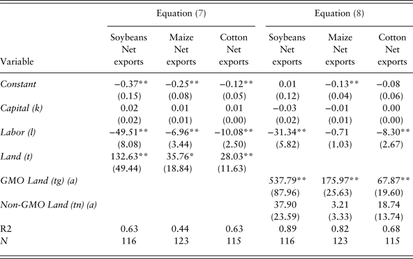
Table 1 reports the baseline cross-country estimates of equation (7) for 2010 (in the first three columns).Footnote 9 As shown, we find that land confers a comparative advantage, and labor confers a comparative disadvantage in each of the three industries.Footnote 10 Further, we find that capital has a negligible supply-side effect on trade. This result seems counterintuitive in that GMO production tends to be capital intensive relative to non-GMO production. We address this issue in Section 5.3 where we consider capital-augmenting technologies that differ across GMO and non-GMO countries.

Positive parameter estimates indicate endowments that confer comparative advantage.
Negative parameter estimates indicate endowments that confer comparative disadvantage.
(a) Parameter estimates on disaggregated endowments indicate the trade effects of converting non-GMO land into GMO land.
Heteroscedasticity-corrected standard errors are in parentheses.
**Significant at the 5% level. *Significant at the 10% level.
What are the effects of land allocations on comparative advantage? Table 1 reports cross-country estimates of equation (8) for 2010 (in the last three columns). As shown, we find that GMO land has a positive effect on net exports in each industry, while the estimates on non-GMO land are insignificant. This result is expected since GMO land is used intensively in GI industries, while non-GMO land is not.Footnote 11 Further, we find large estimates on GMO land. For example, a one million hectare reallocation of land to GMOs results in a $537.79 million increase in net soybean exports; $175.97 million increase in net maize exports; and $67.87 million increase in net cotton exports. These amounts are mean increases across countries in 2010. To provide perspective, a one million hectare increase in GMO land is a modest allocation for large GMO countries, yet represents roughly a doubling of GMO land for emerging GMO countries (see Appendix C).
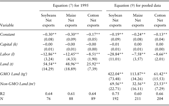
Have the sources of comparative advantage changed over time? Table 2 reports cross-country estimates of equation (7) for 1995 (in the first three columns). We compare these 1995 estimates in Table 2 with the 2010 estimates in Table 1 to assess changes over time in the sources of comparative advantage. We find that land is a source of comparative advantage, and labor is a source of comparative disadvantage both before and after the adoption of GMOs.
Cross-country estimates of equation (7) for 1995, and of equation (9) for 1995 and 2010 pooled data

Notes: Equation (7): Positive parameter estimates indicate endowments that confer comparative advantage.
Negative parameter estimates indicate endowments that confer comparative disadvantage.
Equation (9): Parameter estimates on disaggregated endowments indicate the trade effects of converting non-GMO land into GMO land.
Heteroscedasticity-corrected standard errors are in parentheses.
Heteroscedasticity correction in pooled regressions also correct for residual correlations across 1995 and 2010 for countries.
**Significant at the 5% level. *Significant at the 10% level.
Has the reallocation of land to GMOs changed the patterns of trade over time? Table 2 reports cross-country estimates of equation (9) using pooled data (in the last three columns). These results show the effects of reallocating land from non-GMO to GMO land across time. We find significant positive estimates on both GMO and non-GMO land, with larger magnitudes on GMO land. The results of F-tests reveal that these estimates are statistically different. Recall, GMO land was zero in 1995 and land allocations to GMOs in 2010 vary across countries. We interpret the land allocations in 2010 as ‘reallocations’ because total land endowments do not change much over time.Footnote 12 As such, we conclude that reallocations of land to GMOs increased net exports between 1995 and 2010.
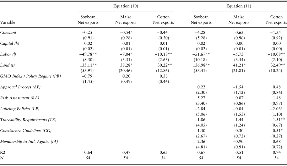
Do stronger GMO policies affect comparative advantage? Table 3 reports cross-country estimates of equations (10) and (11) for 2010. We find that the policy regime has a negligible trade effect, after controlling for capital, labor, and land endowments. This result could reflect an offsetting of any positive and negative effects of the policies comprising the regime. However, we find that component policies have a negligible trade effect for soybeans and maize; while for cotton, traceability requirements confer a comparative advantage, and labeling and coexistence policies confer a comparative disadvantage. To explore further, we apply an F-test to assess the null hypothesis that the parameters on the policies are jointly zero. We find that the null cannot be rejected, suggesting that policies jointly comprising the regime have a negligible trade effect, even for cotton.

Positive parameter estimates indicate endowments that confer comparative advantage.
Negative parameter estimates indicate endowments that confer comparative disadvantage.
Positive parameter estimates on policy variables indicate policies that decrease net costs and increase comparative advantage.
Negative parameter estimates on policy variables indicate policies that increase net costs and decrease comparative advantage.
Heteroscedasticity-corrected standard errors are in parentheses.
**Significant at the 5% level. *Significant at the 10% level.
The above mixed results lead us to ask why select policies have significant estimates for cotton trade (albeit negligible), but not for soybeans and maize. One explanation is that the applicability of regulations varies depending on the intended end use of the product. Whereas soybeans and maize are used primarily as animal feed and as food additives (e.g., soybean oil, high-fructose corn syrup, and corn starch), cotton is used primarily as a fiber.Footnote 13 Crops not intended for food use are not typically reviewed by regulators responsible for food safety. Thus, it is plausible that costs associated with the approval process and risk assessment are relatively low for cotton, and the remaining policies play a more prominent role.Footnote 14 Intuitively the results suggest that traceability policies reduce supply-side costs and increase net exports, while labeling and coexistence policies increase supply-side costs and decrease net exports of cotton.
The more general finding that GMO regulations do not appear to affect trade seems counterintuitive given the literature shows that policies affect bilateral trade and that the use of GMOs can increase productivity (and thus presumably enhance comparative advantage). In contrast to the literature, we examine the supply-side determinants of countries’ net exports to the world (not bilateral trade), so we do not expect to see bilateral tensions associated with policy differences across countries. However, we do expect to see the effects of productivity increases in GMO adopting countries (which tend to have weaker policies).
One possible explanation for our weak policy results is that GMO approvals have occurred in a staggered way over the 16 years of our sample (1995–2010). Indeed, there is considerable variation in the timing of approvals across countries, industries, and traits. For example, the first approval of the herbicide tolerance trait in maize occurred in the US in 1995, Argentina in 1998, and Brazil in 2007. So it is likely that the trade impacts of policies have a varied lag structure across countries and industries, even for mega GMO countries. Thus, we take a conservative approach and conclude that our policy results are early findings in the context of an evolving global policy environment. We also explore extensions in Section 5.3, where we consider the GMO adoption decision as a type of policy, and whether GMO technologies are factor-augmenting and thus lead to increased net exports from GMO adopting countries.
5. Sensitivity analysis
5.1 Land allocations
We perform three sensitivity tests with respect to land allocations. First, we provide a counter-factual experiment for a non-GMO industry. Above, we found a positive relationship between the allocation of land to GMO crops and comparative advantage. This is consistent with HO theory, where a country's net exports in GI industries are intensive in GMO land. We would not expect such a result for a non-GMO crop. Thus, to assess robustness, we re-estimate equation (8) for wheat. Our expectation is that the coefficients on GMO land will be negative for this non-GMO crop (or insignificant). Appendix D reports the findings for wheat that are comparable to those in Table 1. We find that non-GMO land confers comparative advantage for wheat, as expected; while GMO land contributes no explanatory power as its coefficient sign is not well determined. These results support the robustness of earlier findings.
Second, we examine endogeneity that could arise when we disaggregate the land endowment into its GMO and non-GMO components. The intuition for endogeneity is that large net exporters in GI industries tend to have large allocations of GMO land relative to non-GMO land. If trade behavior influences land allocations, we expect an upward bias in the estimate on GMO land and downward bias in the estimate on non-GMO land. Thus, we may conclude that GMO land confers a stronger comparative advantage, and non-GMO land confers a weaker comparative advantage due to bias. However, it is important to note that endogeneity is less likely in our study relative to bilateral trade studies that dominate the literature. In our framework, the trade variable is country net exports to the world (not bilateral trade), and includes GMO and non-GMO content (which varies by country). Further, the measures of GMO and non-GMO land are aggregates (as required by theory) not factor inputs. In this context, it is unlikely that a country's aggregate GMO land is endogenous with respect to net exports in a select industry, which can include GMO and non-GMO varieties. Even so, we take a conservative approach and perform sensitivity analyses.
We use a lagged explanatory variable approach. We re-estimate equation (8) using lagged measures of GMO and non-GMO land. In this experiment, all data are for 2010 except for the land measures which are lagged 12 years (1998), seven years (2003), and two years (2008).Footnote 15 The intuition is that land endowments in earlier years are relatively more exogenous with respect to 2010 trade. If endogeneity is present, we expect the parameter on GMO land to be biased upward and such bias to diminish as the lag increases. Appendix E reports the lagged findings, which can be compared to unlagged findings in Table 1 (last three columns). As shown, the significance patterns are similar across tables, suggesting a stability of results. Interestingly, the estimates on GMO land increase in magnitude as the lag becomes longer. For example, for soybeans the estimate increases from 537.80 to 564.62 to 656.79 to 1,145.48 for 2010, 2008, 2003, and 1998, respectively. This pattern contradicts the effects of endogeneity, and instead suggests that there are lags in trade adjusting to an allocation of land.
Third, we analyze the influence of outlier countries. Based on the above findings, outliers could be early adopters of GMOs.Footnote 16 To assess, we re-estimate equation (8) for 2010 using quantile regression methods. This approach allows us to estimate the conditional median of the trade variable given our explanatory variables, rather than the conditional mean as in ordinary least squares; and it is more robust against outliers in the response variable–net exports. We find that the quantile results are similar in signs and significance as those in Table 1. However, we find that coefficients on GMO land are smaller in magnitude for soybeans and maize, and larger for cotton when we account for outliers. Specifically, when we account for outliers, we find that a one million hectare reallocation of land to GMOs results in a $372.76 million increase in net soybean exports (instead of $537.79), $141.47 million increase in net maize exports (instead of $175.97), and $89.09 million increase in net cotton exports (instead of $67.87).Footnote 17 However, we conclude that even after accounting for outliers, land reallocations to GMOs have a large and significant effect on trade.
5.2 Policies
Next, we assess the robustness of policy results. We begin by analyzing potential endogeneity of policies with respect to trade (using equations (10) and (11)). The intuition is that large net exporters tend to have weak policies (i.e., pro-GMO policies). If policies are endogenous with respect to trade, this would bias (positive and negative) estimates on policies such that they are larger in absolute value. The issue of policy endogeneity in trade studies is typically addressed using either lagged values of the explanatory variables or instrumental variables (IVs). We use a combination, plus a new approach.
First, we use lagged policy measures for 2007, which are exogenous with respect to 2010 trade, assuming no anticipation effects. This approach underlies the Section 4 results. Second, we employ IV methods. We begin by replicating the approach of Vigani et al. (Reference Vigani, Raimondi and Olper2012) in their bilateral trade study.Footnote 18 We instrument each country's policies as the average policies of their five geographically closest neighbors, and conduct Durbin and Wu–Hausman tests. The intuition is that the neighbors’ policies are correlated with the home country's policies, but uncorrelated with the neighbors’ net exports to the world. First-stage regressions show a strong positive correlation between home and neighbor policies (i.e., our instrument is strong).Footnote 19 Further, test results show no evidence of endogeneity for the individual policies or regime (at the 5% level).Footnote 20 We find only one exception – weak evidence of endogeneity of the regime in the case of soybeans (at the 10% level). However, in all cases the second-stage regressions show that estimates on policies are statistically insignificant, consistent with our previous findings. Thus, while Vigani et al. (Reference Vigani, Raimondi and Olper2012) find that GMO policies are endogenous with respect to bilateral trade, we find little evidence that GMO policies are endogenous with respect to net exports.Footnote 21
To assess this issue further, we employ a second IV approach where we instrument each country's GMO regime with an environmental regulation measure developed by Esty and Porter (Reference Esty, Porter, Porter, Sachs and Warner2001).Footnote 22 The intuition is that the environmental regulations of countries are correlated with their GMO policies, but uncorrelated with their net exports to the world.Footnote 23 Our first-stage regressions show that environmental regulations are a strong instrument for the GMO regime.Footnote 24 Again, we perform the Durbin and Wu–Hausman tests and find no evidence of endogeneity of the GMO regime (at the 5% level). Further, the second-stage regressions show that the policy regime is statistically insignificant, consistent with our previous findings. We conclude that our earlier result (that policies have a negligible effect on comparative advantage) is robust.
Third, we examine a political-economy specification, where we consider whether GMO policies determine land allocations. To this end, we redefine the dependent variable in equations (10) and (11) as GMO land, rather than net exports. This analysis is a variation of Table 3. However, we now consider whether policies influence land allocations, while controlling for endowments. We use a lagged-variable approach where we examine the effects of 2007 policies on 2010 land allocations. Appendix F reports the results. We find that the estimates on the policies are insignificant, suggesting that GMO policies do not affect land allocation decisions (on average across countries), after controlling for endowments.
5.3 Technology differences
Next, we consider the robustness of findings with respect to technology differences across countries. The HO model assumes that technologies are identical across countries. However in our application, GMO and non-GMO technologies presumably differ, and countries differ in adoption of GMOs and thus differ in the technologies they tend to employ. The implication of technology differences within the HO model was first addressed in the seminal work of Trefler (Reference Trefler1993, Reference Trefler1995). Trefler (Reference Trefler1995) demonstrates that trade departs from HOV predictions due to ‘factor-augmenting’ technologies.
We consider the role of such technologies in the spirit of Trefler (Reference Trefler1995). We derive a modified HOV expression where technologies can differ across GMO and non-GMO countries (see Appendix G). The new specifications of equations (10) and (11) are:
 $$\eqalign{\left( {x_i - m_i} \right) = &\;\beta _{i0} + {\beta _{i1}} \;G + {\beta _{i2}} \;k + {\beta _{i3}} \;l + {\beta _{i4}} \;t \cr & + {\beta _{i5}} \;{G}\,\cdot \,k + {\beta _{i6}} \;G\,\cdot \,l + {\beta _{i7}} \;G\,\cdot \,t + {\beta _{i8}} \;{\rm PR} + \varepsilon _i}$$
 $$\eqalign{\left({x_i - m_i} \right) = &\;{\beta _{i0}} + {\beta _{i1}} \;G + {\beta _{i2}} \;k + {\beta _{i3}} \;l + {\beta _{i4}} \;t \cr & + {\beta _{i5}} \;G \cdot k + {\beta _{i6}} \;G \cdot l + {\beta _{i7}} \;G \cdot t \cr & + {\beta _{i8}} \;{\rm AP} + {\beta _{i9}} \;{\rm RA} + {\beta _{i10}} \;{\rm LP} + {\beta _{i11}} \;{\rm TR} + {\beta _{i12}} \;{\rm CG} + {\beta _{i13}} \;{\rm IA} + \varepsilon _i}$$
where G is a dummy variable that equals 1 if the country adopts GMOs and 0 otherwise; ε i is a randomly distributed error term; and all other variables are as previously defined.
In equations (12) and (13), the coefficients are effective Rybczynski coefficients (ERCs) defined as the product of the standard Rybczynski coefficients (α) and factor-augmenting technologies (π). In other words, β i = α iπ. We expect ERCs to vary across GMO and non-GMO countries if factor-augmenting technologies differ across these groups. The interaction terms in equations (12) and (13) allow us to examine differences in ERC's for GMO countries relative to non-GMO countries. Our a priori expectation is that ERCs will be larger in absolute value for GMO countries if GMO technologies are factor augmenting.
Appendix H reports cross-country estimates of equations (12) and (13) for 2010. Findings show patterns consistent with Table 3, where land confers a comparative advantage and labor confers a comparative disadvantage. However, we now see that land confers a particularly strong comparative advantage in GMO countries (for soybeans and cotton) and labor confers a particularly strong comparative disadvantage in non-GMO countries (for maize and cotton). This suggests that GMO technologies are land and labor augmenting. Further, we see that capital is a source of comparative disadvantage for non-GMO countries (in soybean and maize), but is a source of comparative advantage for GMO countries (in maize). This suggests that GMO technologies are capital augmenting and strong enough to reverse net trade (for maize). This result differs from our previous finding that capital has a negligible trade effect. The new results are more consistent with the literature, which shows GMO crops to be capital intensive.Footnote 25
Finally, Appendix H shows that policies still have little effect on comparative advantage, after controlling for endowments and technologies. One exception is that traceability requirements have a positive trade effect for cotton, consistent with the results in Table 3. The second exception is that coexistence guidelines have a positive trade effect for maize, a result not shown in Table 3. This later finding likely reflects the influence of countries such as Argentina and France who are exceptionally large net exporters of maize and have strong coexistence guidelines (see Appendix C).Footnote 26 However, all of the remaining estimates on policy instruments are insignificant. Thus, allowing for factor-augmenting technologies does not alter our previous conclusion that these policies have a negligible supply-side effect on trade.
It is plausible that the policy results are weak because the critical policy decision is whether to allow GMO technologies in production or not, and this ‘adoption decision’ may overshadow the regulation of GMOs once in the market. Further, it is plausible that the (zero-one) technology adoption decision is related to the (continuous) land allocation decision, since countries differ in adoption of GMOs and consequently differ in the technologies they tend to employ. Thus, our finding that technologies play a role in augmenting land productivity likely reflects the effects of the technology adoption decision (a type of policy).
To consider this issue further, we first examine correlations between the GMO dummy (i.e., adoption decision), GMO land (i.e., allocation decision), and GMO policies (i.e., policy instruments). We find these correlations are modest and take the expected signs.Footnote 27 The strongest correlation is between GMO land and the GMO dummy (0.34), suggesting a positive relationship between the adoption and land allocation decisions. We then re-estimate the regressions where land is disaggregated into its GMO and non-GMO components (i.e., Table 1), but now include the GMO dummy to control for the adoption decision. Appendix I reports the findings. As shown, the core results are insensitive to the inclusion of the dummy. That is, the land allocation decision has strong explanatory power, even after controlling for the GMO adoption decision. One possible explanation is that land allocations are based (in part) on matching GMO traits with exogenously determined land and weather attributes. For example, adoption of salt or drought tolerant crops addresses specific environmental features. These exogenous features likely determine the magnitude of land allocations following an adoption decision.
In summary, we conclude that the policy dimension that matters most is the decision of whether to adopt GMOs or not, rather than the regulation of GMOs once in the market. We also conclude that there is a modest correlation between GMO adoption and land allocations, suggesting these decisions are to some extent interrelated.
5.4 Other issues
We consider two remaining issues. First, we consider the robustness of results with respect to cross-time factors. To this end, we re-estimate equation (9) using pooled data across 1995 and 2010, and include a time fixed effect. We find that the parameter signs, relative magnitudes, and fit of the regressions are stable. That is, our results are robust with respect to unobserved cross-time factors that may affect trade. Finally, we assess robustness with respect to choice of variable measures. To this end, we construct multiple measures of capital, labor, and land.Footnote 28 We find that the results are robust with respect to choice of measure. The results reported are those generated using the measures that match most closely with the underlying theory definition of endowments.
6. Concluding remarks
This paper provides empirical evidence on the supply-side determinants of trade in the GMO-intensive industries of soybeans, maize, and cotton during the time periods before and after the advent of GMOs. Five conclusions emerge. First, we found that land endowments have a positive supply-side effect on trade, and labor endowments have a negative trade effect. Second, we found that the allocation of land to GMO crops has a positive effect on trade. For example, a one million hectare allocation of land to GMO crops results in a $537.79 million increase in net soybean exports (on average across countries). The economic significance of this effect is particularly large for emerging GMO countries. Third, we found that land is a source of comparative advantage and labor is a source of comparative disadvantage both before and after the advent of GMOs. We also found that the reallocation of land to GMOs substantially increased the net exports of countries between 1995 and 2010. In other words, our first two conclusions hold both across countries at one point in time, and also across time from 1995 to 2010. Fourth, we found that the GMO policy regime and individual policies of countries appear to have a negligible effect on trade (on average across countries).
These finding are robust to a variety of considerations. First, using a counter-factual approach, we examined whether our findings would reverse for a non-GMO industry such as wheat. As expected, we found that non-GMO land serves as a determinant of trade for wheat, while GMO land does not. Second, using a lagged explanatory variable approach, we examined the potential endogeneity of countries’ land allocation decisions with respect to their trade. We found no evidence of this form of endogeneity. To the contrary, we found that past land allocations serve as a strong determinant of future comparative advantage. Third, using quantile regression methods, we analyzed the influence of outlier countries (such as early adopters of GMOs). We found that after accounting for outliers, land reallocations to GMOs continue to have a significant effect on comparative advantage. Fourth, we considered the potential endogeneity of policies with respect to trade. Using a lagged variable approach and two IV approaches, we found scant evidence of policy endogeneity. Fifth, using a political economy approach, we examined whether policies influence land allocation decisions between GMOs and non-GMOs. We found no evidence that policies affect land allocations (on average across countries). Finally, we examined the robustness of results when we allow for technology differences across GMO and non-GMO countries. We found that our earlier results are robust; however, we also found that GMO technologies are factor augmenting in some cases. For example, we found that GMO technologies tend to be land and labor augmenting; and are also capital augmenting and strong enough to reverse net trade (for maize).
Our findings point to a puzzle: Why do land allocations affect comparative advantage, while policies have a negligible effect on land allocations and on comparative advantage? One explanation is that the global policy setting in 2010 was evolving with considerable uncertainty. As a by-product, there may be a substantial lag in the effects of policies on land allocations and net exports. Yet another explanation is that policy stringency can both increase and decrease supply-side costs (and thus have a negligible net effect). Weak GMO policies may reduce supply-side costs because policy-compliance costs are lower. At the same time, weak GMO policies may increase supply-side costs because of the costs associated with creating transparency around product characteristics are higher. For example, producers may incur costs associated with voluntary labeling even in the absence of mandatory labeling regulations. Further, it is plausible that GMO policies effect supply-side costs for both GMO and non-GMO producers in the same direction. For example, strong coexistence guidelines could increase supply-side costs for both GMO and non-GMO producers. Finally, it is plausible that the policy results are weak because the critical policy decision is whether to allow GMO technologies or not, and this decision overshadows the regulation of GMOs once in the market. These issues point to the need for further research on the interactions of policies and the cost effects of alternative combinations. Such research may become feasible as measures of GMO policies and GMO trade are further developed and refined.
Supplementary material
To view supplementary material for this article, please visit https://doi.org/10.1017/S1474745617000180