



%20--%3e%3c!DOCTYPE%20svg%20PUBLIC%20'-//W3C//DTD%20SVG%201.0//EN'%20'http://www.w3.org/TR/2001/REC-SVG-20010904/DTD/svg10.dtd'%3e%3csvg%20version='1.0'%20id='Layer_1'%20xmlns='http://www.w3.org/2000/svg'%20xmlns:xlink='http://www.w3.org/1999/xlink'%20x='0px'%20y='0px'%20width='64px'%20height='64px'%20viewBox='5.5%20-3.5%2064%2064'%20enable-background='new%205.5%20-3.5%2064%2064'%20xml:space='preserve'%3e%3cg%3e%3ccircle%20fill='%23FFFFFF'%20fill-opacity='0'%20cx='37.785'%20cy='28.501'%20r='28.836'/%3e%3cpath%20fill='%23595959'%20d='M37.441-3.5c8.951,0,16.572,3.125,22.857,9.372c3.008,3.009,5.295,6.448,6.857,10.314%20c1.561,3.867,2.344,7.971,2.344,12.314c0,4.381-0.773,8.486-2.314,12.313c-1.543,3.828-3.82,7.21-6.828,10.143%20c-3.123,3.085-6.666,5.448-10.629,7.086c-3.961,1.638-8.057,2.457-12.285,2.457s-8.276-0.808-12.143-2.429%20c-3.866-1.618-7.333-3.961-10.4-7.027c-3.067-3.066-5.4-6.524-7-10.372S5.5,32.767,5.5,28.5c0-4.229,0.809-8.295,2.428-12.2%20c1.619-3.905,3.972-7.4,7.057-10.486C21.08-0.394,28.565-3.5,37.441-3.5z%20M37.557,2.272c-7.314,0-13.467,2.553-18.458,7.657%20c-2.515,2.553-4.448,5.419-5.8,8.6c-1.354,3.181-2.029,6.505-2.029,9.972c0,3.429,0.675,6.734,2.029,9.913%20c1.353,3.183,3.285,6.021,5.8,8.516c2.514,2.496,5.351,4.399,8.515,5.715c3.161,1.314,6.476,1.971,9.943,1.971%20c3.428,0,6.75-0.665,9.973-1.999c3.219-1.335,6.121-3.257,8.713-5.771c4.99-4.876,7.484-10.99,7.484-18.344%20c0-3.543-0.648-6.895-1.943-10.057c-1.293-3.162-3.18-5.98-5.654-8.458C50.984,4.844,44.795,2.272,37.557,2.272z%20M37.156,23.187%20l-4.287,2.229c-0.458-0.951-1.019-1.619-1.685-2c-0.667-0.38-1.286-0.571-1.858-0.571c-2.856,0-4.286,1.885-4.286,5.657%20c0,1.714,0.362,3.084,1.085,4.113c0.724,1.029,1.791,1.544,3.201,1.544c1.867,0,3.181-0.915,3.944-2.743l3.942,2%20c-0.838,1.563-2,2.791-3.486,3.686c-1.484,0.896-3.123,1.343-4.914,1.343c-2.857,0-5.163-0.875-6.915-2.629%20c-1.752-1.752-2.628-4.19-2.628-7.313c0-3.048,0.886-5.466,2.657-7.257c1.771-1.79,4.009-2.686,6.715-2.686%20C32.604,18.558,35.441,20.101,37.156,23.187z%20M55.613,23.187l-4.229,2.229c-0.457-0.951-1.02-1.619-1.686-2%20c-0.668-0.38-1.307-0.571-1.914-0.571c-2.857,0-4.287,1.885-4.287,5.657c0,1.714,0.363,3.084,1.086,4.113%20c0.723,1.029,1.789,1.544,3.201,1.544c1.865,0,3.18-0.915,3.941-2.743l4,2c-0.875,1.563-2.057,2.791-3.541,3.686%20c-1.486,0.896-3.105,1.343-4.857,1.343c-2.896,0-5.209-0.875-6.941-2.629c-1.736-1.752-2.602-4.19-2.602-7.313%20c0-3.048,0.885-5.466,2.658-7.257c1.77-1.79,4.008-2.686,6.713-2.686C51.117,18.558,53.938,20.101,55.613,23.187z'/%3e%3c/g%3e%3c/svg%3e)
%20--%3e%3c!DOCTYPE%20svg%20PUBLIC%20'-//W3C//DTD%20SVG%201.0//EN'%20'http://www.w3.org/TR/2001/REC-SVG-20010904/DTD/svg10.dtd'%3e%3csvg%20version='1.0'%20id='Layer_1'%20xmlns='http://www.w3.org/2000/svg'%20xmlns:xlink='http://www.w3.org/1999/xlink'%20x='0px'%20y='0px'%20width='64px'%20height='64px'%20viewBox='5.5%20-3.5%2064%2064'%20enable-background='new%205.5%20-3.5%2064%2064'%20xml:space='preserve'%3e%3cg%3e%3ccircle%20fill='%23FFFFFF'%20fill-opacity='0'%20cx='37.637'%20cy='28.806'%20r='28.276'/%3e%3cg%3e%3cpath%20fill='%23595959'%20d='M37.443-3.5c8.988,0,16.57,3.085,22.742,9.257C66.393,11.967,69.5,19.548,69.5,28.5c0,8.991-3.049,16.476-9.145,22.456%20C53.879,57.319,46.242,60.5,37.443,60.5c-8.649,0-16.153-3.144-22.514-9.43C8.644,44.784,5.5,37.262,5.5,28.5%20c0-8.761,3.144-16.342,9.429-22.742C21.101-0.415,28.604-3.5,37.443-3.5z%20M37.557,2.272c-7.276,0-13.428,2.553-18.457,7.657%20c-5.22,5.334-7.829,11.525-7.829,18.572c0,7.086,2.59,13.22,7.77,18.398c5.181,5.182,11.352,7.771,18.514,7.771%20c7.123,0,13.334-2.607,18.629-7.828c5.029-4.838,7.543-10.952,7.543-18.343c0-7.276-2.553-13.465-7.656-18.571%20C50.967,4.824,44.795,2.272,37.557,2.272z%20M46.129,20.557v13.085h-3.656v15.542h-9.944V33.643h-3.656V20.557%20c0-0.572,0.2-1.057,0.599-1.457c0.401-0.399,0.887-0.6,1.457-0.6h13.144c0.533,0,1.01,0.2,1.428,0.6%20C45.918,19.5,46.129,19.986,46.129,20.557z%20M33.042,12.329c0-3.008,1.485-4.514,4.458-4.514s4.457,1.504,4.457,4.514%20c0,2.971-1.486,4.457-4.457,4.457S33.042,15.3,33.042,12.329z'/%3e%3c/g%3e%3c/g%3e%3c/svg%3e)
1. Introduction
A vertical natural convection boundary layer (NCBL) is a fluid motion driven by buoyancy along a vertical wall when the ambient fluid temperature is different from the wall temperature. The laminar NCBL has been investigated extensively over the past several decades where the exact solutions are available (e.g. Illingworth Reference Illingworth1950; Schetz & Eichhorn Reference Schetz and Eichhorn1962). However, many industrial and geophysical NCBL flows operate beyond this thoroughly understood laminar regime at a much higher Grashof number where the flow transitions to turbulence.
Most previous literature distinguishes the onset of turbulence by examining the mean statistics and their trends with the development of the flow. In an early experimental investigation, Cheesewright (Reference Cheesewright1968) reported mean statistics for a spatially developing NCBL up to  $Gr_x=10^{11}$. Here,
 $Gr_x=g\beta \theta _w x^3/\nu ^2$ is the Grashof number based on the downstream distance
 $x$, where
 $g$ is the gravitational acceleration,
 $\theta _w$ is the temperature difference between the isothermal wall and the ambient,
 $\beta$ represents the thermal expansion coefficient, and
 $\nu$ denotes the kinematic viscosity of the fluid. By examining the velocity and temperature fluctuations, Cheesewright (Reference Cheesewright1968) identified the onset of laminar–turbulent transition at
 $Gr_x = 2\times 10^9$, and the beginning of the turbulent regime at
 $Gr_x= 2\times 10^{10}$. In the turbulent regime, the Nusselt number, which characterises the wall heat transfer rate of the flow, was found to follow a 0.33 power law with Grashof number as suggested by Bayley (Reference Bayley1955). Similar results were also seen in Warner & Arpaci (Reference Warner and Arpaci1968), where the NCBL was considered turbulent for
 $Gr_x>8\times 10^9$ based on their thermocouple measurements up to
 $Gr_x=10^{11}$. Siebers, Moffatt & Schwind (Reference Siebers, Moffatt and Schwind1985) studied the heat transfer characteristics of a turbulent NCBL up to
 $Gr_x=10^{12}$, with maximum temperature difference
 $500\,^\circ {\rm C}$. Their measurements showed that the laminar–turbulent transition is greatly affected by the variations in fluid properties due to large temperature differences, and the heat transfer in the turbulent regime follows a
 $1/3$ power law with a reference temperature correction. Tsuji & Nagano (Reference Tsuji and Nagano1988a) investigated a spatially developing turbulent NCBL with detailed experiment measurements for turbulence statistics up to
 $Gr_x = 1.8\times 10^{11}$. Using the experiment data, Tsuji & Nagano (Reference Tsuji and Nagano1988a) found that their spatially developing NCBL undergoes transition at
 $Gr_x\approx 8\times 10^8$, and a turbulent regime was identified for
 $Gr_x> 7\times 10^{9}$ based on the mean velocity and temperature profiles. Their measurements of the Nusselt number in the turbulent regime were found to follow an empirical
 $1/3$ power law correlation with the Grashof number, which is consistent with studies in the similar Grashof number range (
 $Gr_x < O(10^{11})$; Saunders Reference Saunders1936, Reference Saunders1939; Bayley Reference Bayley1955; Cheesewright Reference Cheesewright1968; Siebers et al. Reference Siebers, Moffatt and Schwind1985; Nakao, Hattori & Suto Reference Nakao, Hattori and Suto2017). Their work was extended further by Tsuji & Nagano (Reference Tsuji and Nagano1989), who related empirically the boundary layer thickness
 $\delta$ to the downstream distance
 $x$. This
 $\delta$–
 $x$ correlation enables the comparison between statistically steady NCBL flows and the temporally evolving periodic flows by matching the boundary layer thickness. Abedin, Tsuji & Hattori (Reference Abedin, Tsuji and Hattori2009) compared their direct numerical simulations (DNS) for a temporally developing NCBL with the measurements of Tsuji & Nagano (Reference Tsuji and Nagano1988a) by matching the boundary layer thickness at
 $Gr_{\delta }=5.94\times 10^6$. Although initial conditions were shown to have significant effects on the turbulence statistics in their study, the ensemble average of multiple DNS with different initialisations showed good agreement with the data of Tsuji & Nagano (Reference Tsuji and Nagano1988a). To date, most existing studies for turbulent vertical NCBLs sit within the range from
 $Gr_\delta =2\times 10^5$ (equivalently,
 $Gr_x = 10^9$ for spatially developing measurements) to
 $Gr_\delta = 6.5\times 10^{6}$ (equivalently,
 $Gr_x = 10^{11}$).
More recently, evidence suggests that the turbulent NCBL flow immediately after the laminar–turbulent transition has a laminar near-wall flow with a turbulent outer shear layer (e.g. Wells & Worster Reference Wells and Worster2008; Ng et al. Reference Ng, Ooi, Lohse and Chung2015, Reference Ng, Ooi, Lohse and Chung2017). This is consistent with the idea of an ultimate turbulent regime that has been well developed in Rayleigh–Bénard convection (Grossmann & Lohse Reference Grossmann and Lohse2000, Reference Grossmann and Lohse2011), where the development of turbulence is comprised of two stages: a background-dominated regime where the flow is in fact a laminar boundary layer driven by a turbulent bulk ‘wind’, and an ultimate regime where both boundary layer and the bulk ‘wind’ are fully turbulent. In the context of vertical convection flows, the transition towards the ultimate regime for turbulent NCBL flows indeed requires the near-wall laminar-like boundary layer to evolve into a fully turbulent one (Kraichnan Reference Kraichnan1962; Grossmann & Lohse Reference Grossmann and Lohse2000, Reference Grossmann and Lohse2011). However, while the turbulence statistics of the turbulent NCBL have been well documented for flows at laboratory scale (i.e. 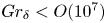 $Gr_{\delta }< O(10^7)$), significantly fewer data extend to sufficiently high Grashof number to see a transition to the ultimate regime. Therefore, the extent and characteristics of the initial laminar-like turbulent regime, as well as the details of this transition towards the ultimate regime, are not well understood. Ng et al. (Reference Ng, Ooi, Lohse and Chung2015) studied numerically the natural convection with Prandtl number
 $Pr=0.709$ in a differentially heated channel up to a channel-width-based Grashof number
 $Gr_H=1.41\times 10^{9}$. In their analysis, they treated the NCBL in two separate parts – an outer bulk flow driven by a turbulent ‘wind’, and an inner boundary layer. Using DNS data, they showed that although the outer bulk flow is identified as fully developed turbulence, the inner boundary layer could still be laminar-like and follows a Prandtl–Blasius–Pohlhausen scaling. This multi-layer approach for the turbulent NCBL conveniently distinguishes the near-wall characteristics from the bulk flow behaviour where the viscous force and molecular diffusion are negligible, and allows asymptotic matching between the layers to give explicit expressions for the mean temperature and velocity profiles (George & Capp Reference George and Capp1979; Hölling & Herwig Reference Hölling and Herwig2005; Shiri & George Reference Shiri and George2008). Their work was later extended by Ng et al. (Reference Ng, Ooi, Lohse and Chung2017), where the authors conditionally averaged the turbulence statistics based on high- and low-shear patches in the near-wall region, and recovered a 0.37 power law for the Nusselt number correlation in high-shear events. With increasing Grashof number, Ng et al. (Reference Ng, Ooi, Lohse and Chung2017) showed that the high-shear patches occupy increasingly larger portions of the wall areas, and suggested that the flow would transition to an ultimate shear-dominated regime at higher Grashof number. A similar idea is seen in Wells & Worster (Reference Wells and Worster2008), where they conceptually decomposed a spatially developing NCBL into a two-layer structure in their theoretical analysis. Based on empirical correlations for the forced flow, and making use of the measurements of Tsuji & Nagano (Reference Tsuji and Nagano1988a,Reference Tsuji and Naganob), Wells & Worster (Reference Wells and Worster2008) suggested that the turbulent NCBL would have two distinct stages as the flow progressively becomes more turbulent: at relatively low Grashof number, the flow is dominated by the near-wall buoyancy as in Tsuji & Nagano (Reference Tsuji and Nagano1988a), whereas at higher Grashof number, the flow would be dominated by inertia since the near-wall buoyancy grows thin. Using a Reynolds analogy, Wells & Worster (Reference Wells and Worster2008) further suggested that the Nusselt number at asymptotically high Grashof number (
 $Gr_{\delta }>O(10^{11})$) would follow a
 $1/2$ power law.
In temporally developing periodic DNS, Ke et al. (Reference Ke, Williamson, Armfield, Norris and Komiya2020) demonstrated that for  $Gr_{\delta }> 10^7$, the NCBL flow would become fully turbulent such that a universal buoyancy-modified log law is obtained, whereas at relatively low Grashof number
 $10^6< Gr_{\delta }<10^7$, where the NCBL is generally thought to be turbulent in the literature, the flow is still transitional or weakly turbulent. Ke et al. (Reference Ke, Williamson, Armfield, Komiya and Norris2021) further explored the flow characteristics and turbulence structures by separating the turbulent flow into a near-wall boundary-layer-like region and an outer plume-like region using the maximum mean streamwise velocity location
 $\delta _m$. In the fully turbulent regime, there exists a constant heat flux layer (e.g. George & Capp Reference George and Capp1979; Hölling & Herwig Reference Hölling and Herwig2005) and a constant forcing layer in the near-wall region, while the outer plume-like region appears self-similar and can be well modelled by an integral plume model (cf. Morton, Taylor & Turner Reference Morton, Taylor and Turner1956; Cooper & Hunt Reference Cooper and Hunt2010). Using DNS data, Ke et al. (Reference Ke, Williamson, Armfield, Komiya and Norris2021) showed that the local heat transfer in the plume-like region exhibits a
 $1/2$ power law to the local plume Grashof number, similar to the asymptotic heat transfer in Grossmann & Lohse (Reference Grossmann and Lohse2000) and Wells & Worster (Reference Wells and Worster2008), while the overall Nusselt number would follow a fully turbulent scaling with logarithmic correction due to the near-wall kinetic boundary layer (resulting in a 0.381 power law for
 $10^7< Gr_\delta <1.2\times 10^8$), consistent with Grossmann & Lohse (Reference Grossmann and Lohse2011) and Ng et al. (Reference Ng, Ooi, Lohse and Chung2017). The authors also noted that the departure from the empirical
 $1/3$ power law to the slightly higher 0.381 power scaling at
 $Gr_{\delta }>10^7$ is very subtle and gradual. A similar multi-layer approach is also seen in Wei, Wang & Abraham (Reference Wei, Wang and Abraham2021a,Reference Wei, Wang and Abrahamb), where, using the measurements of Tsuji & Nagano (Reference Tsuji and Nagano1988a,Reference Tsuji and Naganob), they showed that the near-wall region of the NCBL is similar to that of a differentially heated channel flow, while the outer part of the NCBL is similar to that of a turbulent planar plume. Howland et al. (Reference Howland, Ng, Verzicco and Lohse2022) studied natural convection in differentially heated channels at high Prandtl numbers using DNS. Following Wells & Worster (Reference Wells and Worster2008), they used empirical relations for the forced flows to estimate the Prandtl number dependence on the transition to the shear-driven ultimate regime. So far, investigations on the turbulence development in the relatively low Grashof number regime has been limited since the turbulent flow at this stage appears transitional or weakly turbulent, largely dependent on the initial conditions. Early studies did not differentiate between a fully turbulent NCBL and the one that is turbulent in the outer plume-like region but laminar in the near-wall region – hereafter, the ‘classical’ turbulent regime, since most early studies would seem to be in this regime based on their turbulence statistics (see § 3.1), given their subtle difference in the Nusselt number scaling and lack of direct measurements of high Grashof number flows with which to compare. Now that fully turbulent results have been obtained, it is possible to re-examine the near-wall mechanics on the ‘classical’ weakly turbulent regime and clarify how and when near-wall transition takes place.
The present study investigates a turbulent NCBL flow with Prandtl number 0.71 using periodic temporally developing DNS, focusing on the development of turbulence in such a ‘classical’ turbulent regime. By comparing the turbulence statistics in § 3.1 and the premultiplied power spectra in § 3.2, we will show that the near-wall region is initially laminar-like, and the turbulent NCBL is indeed driven by the bulk plume-like structures. Using a dimensionless length scale, the extent of the ‘classical’ turbulent regime can be identified in § 3.3. In this regime, the skin friction coefficient follows a laminar-like scaling as in Blasius boundary layers, whereas at higher Grashof number, the flow appears initial-condition-invariant, and the skin friction converges to a more complicated log-law-type behaviour. In § 3.4, we explore the development of the near-wall turbulence by examining the turbulence kinetic energy budget in both the ‘classical’ and fully turbulent ultimate regimes. Section 4 briefly concludes the findings in this paper.
2. Mathematical description
The evolution of the incompressible natural convection flow is comprised of the conservation equations of mass, momentum and thermal energy. With the Boussinesq approximation, the governing equations read
 \begin{gather} \frac{\partial u_i}{\partial x_i} = 0, \end{gather}
 \begin{gather}\frac{\partial u_i}{\partial t}+\frac{\partial u_i u_j}{\partial x_j} ={-}\frac{1}{\rho}\,\frac{\partial p}{\partial x_i}+\nu\,\frac{\partial^2 u_i}{\partial {x_j}^2}+ g\beta\theta\delta_{i1}, \end{gather}
 \begin{gather}\frac{\partial \theta}{\partial t}+\frac{\partial u_j \theta}{\partial x_j} = \kappa\,\frac{\partial^2 \theta}{\partial {x_j}^2}, \end{gather}
where the subscripts  $i,j=1,2,3$ denote the velocity field
 $u$ in the
 $x$ (streamwise),
 $y$ (wall-normal) and
 $z$ (spanwise) directions. In (2.1),
 $\rho$ is the density of the fluid,
 $g$ represents the projection of the gravitational vector pointing in the negative
 $x$ direction,
 $\theta = T-T_\infty$ is the temperature difference between the local temperature
 $T$ and the far-field temperature
 $T_\infty$, and
 $\delta _{i1}$ is the Kronecker delta. Also,
 $\beta$,
 $\kappa$ and
 $\nu$ are the fluid properties: the thermal expansion coefficient, the thermal diffusivity and the kinematic viscosity, respectively. For the problem under consideration, the working fluid is considered as air with Prandtl number
 $Pr \equiv \nu /\kappa = 0.71$.
To allow a spatially invariant, temporal flow to develop, periodic boundary conditions are applied in the streamwise and spanwise directions. For the wall-normal direction, no-slip and no-permeability conditions are imposed on the isothermal wall ( $\theta =\theta _w$ at
 $y=0$) and a slip wall boundary is applied in the quiescent far field (
 $\theta = 0$ at
 $y=\infty$).
With these boundary conditions, the flow system (2.1) has a laminar analytical solution (Illingworth Reference Illingworth1950; Schetz & Eichhorn Reference Schetz and Eichhorn1962) that reads
 \begin{gather} u(\eta) = \frac{4g\beta\theta_w t}{1-Pr}\left[\text{i}^2\text{erfc}(\eta)-\text{i}^2\text{erfc}\left(\frac{\eta}{\sqrt{Pr}}\right)\right], \end{gather}
 \begin{gather}\theta(\eta) = \theta_w\,\text{erfc}(\eta), \end{gather}
where  $u$ is the streamwise velocity (note that the parallel flow is streamwise- and spanwise-invariant),
 $\text {erfc}(\eta )$ is the complementary error function of the similarity coordinate
 $\eta =y/\sqrt {4\kappa t}$, and
 $\text {i}^n\text {erfc}(\eta )$ represents the
 $n$th integral of the complementary error function:
 $\text {ierfc}(\eta )= \int ^\infty _\eta \text {erfc}(\eta )\,\mathrm {d}\eta =\exp (-\eta ^2)/\sqrt {{\rm \pi} }-\eta \,\text {erfc}(\eta )$ and
 $\text {i}^2\text {erfc}(\eta ) = (\text {erfc}(\eta )-2\eta \,\text {ierfc}(\eta ))/4$.
To encourage a three-dimensional transition to turbulence, the laminar temperature field (2.2b) is also augmented with a perturbation, such that the initial temperature field  $\theta _0$ is given by
 \begin{equation} \theta_0(x,y,z) = {\theta}(y) + \tilde{\theta}(x,y,z), \end{equation}
where  $\theta (y)$ is the laminar analytical solution obtained from (2.2b), the perturbation
 $\tilde {\theta }(x,y,z)$ is defined by
 \begin{equation} \tilde{\theta}(x,y,z) = A_0 [\text{RAND}(0,1)-0.5], \end{equation}
 $A_0=1$ denotes the magnitude of the background white noise, and
 $\text {RAND}(0,1)$ is a statistically uniform random number generator between 0 and 1. The flow is initialised using the velocity analytical solution (2.2a) and the perturbed temperature field (2.3) at
 $Gr_{\delta _0} = 705$. Here, the Grashof number
 $Gr_{\delta }$ and the integral velocity boundary layer thickness
 $\delta$ are given as
 \begin{equation} Gr_{\delta}\equiv \frac{g\beta \theta_w \delta^3}{\nu^2},\quad \delta \equiv \int^{\infty}_{0} \frac{\bar{u}}{\bar{u}_m} \,\mathrm{d} y, \end{equation}
where  $\bar {u}$ represents the mean (spatial average) quantity of the streamwise velocity
 $u$ in the homogeneous
 $x$–
 $z$ plane, and
 $\bar {u}_m$ denotes the maximum mean streamwise velocity. Note that our temporally developing NCBL is streamwise- and spanwise-invariant such that the boundary layer thickness
 $\delta$ and Grashof number
 $Gr_{\delta }$ are proxies for the flow development time
 $t$, as shown in figure 1. Although the magnitude of initial noise
 $A_0=1$ is relatively large, the artificial temperature perturbation decays rapidly via the receptivity process after a few iterations, and the noise modes in the laminar regime grow linearly in accordance with linear stability results before they undergo nonlinear amplification (Ke et al. Reference Ke, Williamson, Armfield, McBain and Norris2019).
The Grashof number  $Gr_{\delta }$ evolution of the NCBL (for DNS-D) with the flow development time
 $t/t_s$, where
 $t_s=\kappa ^{1/3}/(g\beta \theta _w)^{2/3}$ is the intrinsic time scale.

The DNS are carried out on a Cartesian finite volume grid, with a uniform mesh in the homogeneous directions (streamwise and spanwise), while the wall-normal direction employs a logarithmically stretched mesh using a gamma function (table 1). The grid sizes are determined so that they are able to resolve the Kolmogorov scales by the end of the simulation (cf. Ng et al. Reference Ng, Ooi, Lohse and Chung2015; Williamson et al. Reference Williamson, Armfield, Kirkpatrick and Norris2015), with  $\Delta x \approx \Delta z \approx 2.5 \eta _k$ in the homogeneous directions, and
 $\Delta y_{min}\approx 0.3\eta _k$ and
 $\Delta y_{max}\approx 6.4 \eta _k$ in the wall-normal direction. Here,
 $\eta _k= (-\nu ^3/\varepsilon )^{1/4}$ is the Kolmogorov length scale, and
 $\varepsilon =-\nu \,\overline {(\partial u_i^{\prime }/\partial x_j)}$ is the turbulent dissipation. In the following analysis, we also include the DNS data that have been reported previously in Ke et al. (Reference Ke, Williamson, Armfield, Norris and Komiya2020, Reference Ke, Williamson, Armfield, Komiya and Norris2021) for comparison; the detailed initial conditions for these simulations are listed in table 2. We will show in § 3 that these initial conditions are responsible for different transition pathways that the NCBLs undergo, but have minimal effect on the flow statistics once the flow becomes fully turbulent in the ultimate regime.
Simulation parameters for the present study (DNS-D). Here,  $L_s= \kappa ^{2/3}/(g\beta \theta _w)^{1/3}$ is the intrinsic length scale,
 $\delta _f$ represents the velocity integral thickness by the end of the simulation,
 $\varDelta ^{\eta _k}$ and
 $\varDelta ^+$ denote the grid size in Kolmogorov scale and wall units by the end of the simulation, with the subscripts
 $min$ and
 $max$ indicating the smallest grid (first grid on the wall) and the largest grid (far field).

Initial conditions for the DNS dataset. Here,  $\tilde {\theta }_{xz}$ is a discrete sinusoidal perturbation in both the streamwise and spanwise directions (cf. Ke et al. Reference Ke, Williamson, Armfield, Norris and Komiya2020).

In the present study, the turbulence statistics of our temporally developing NCBL are compared with the spatially developing NCBL flows (Tsuji & Nagano Reference Tsuji and Nagano1988a; Nakao et al. Reference Nakao, Hattori and Suto2017) by matching the boundary layer thickness  $\delta$. This method has also been adopted by a number of studies for the temporally developing NCBL (Abedin et al. Reference Abedin, Tsuji and Hattori2009; Ke et al. Reference Ke, Williamson, Armfield, Norris and Komiya2020, Reference Ke, Williamson, Armfield, Komiya and Norris2021). It is noted that for spatially developing NCBL flows, statistics are normally obtained by taking the temporal average since the flow is steady in the mean, whereas for our temporally developing NCBL, the parallel flow is unsteady in the mean and the statistics are obtained by averaging over the homogeneous
 $x$–
 $z$ plane.
3. Results and discussion
The characteristics of high Grashof number flows that transition to the ultimate regime have been investigated extensively in our earlier analyses (Ke et al. Reference Ke, Williamson, Armfield, Norris and Komiya2020, Reference Ke, Williamson, Armfield, Komiya and Norris2021), and we will focus primarily on the ‘classical’ (weakly turbulent) regime in the following analysis.
Before proceeding to the detailed analysis, a rigorous identification of the near-wall region is needed. Following our earlier analysis (Ke et al. Reference Ke, Williamson, Armfield, Komiya and Norris2021), we identify the near-wall and outer bulk region of the NCBL flow by the maximum mean streamwise velocity location  $\delta _m$. This wall-normal location distinguishes turbulence behaviours in the two shear layers of the NCBL: figure 2 shows the ratio of the streamwise (
 $\lambda _f$) to the spanwise (
 $\lambda _g$) Taylor microscale, which are obtained by using the mean autocorrelation in the respective directions, at three Grashof numbers in the turbulent regime (
 $Gr_{\delta }>10^6$ for DNS-D; see § 3.1). Beyond the maximum mean streamwise velocity location (
 $y>\delta _m$),
 $\lambda _f/\lambda _g \approx \sqrt {2}$ is approximately constant for all data shown in figure 2, indicating that the flow in this region is isotropic due to strong turbulent mixing (Pope Reference Pope2001), whereas in the near-wall region (
 $y<\delta _m$),
 $\lambda _f/\lambda _g$ grows with
 $Gr_{\delta }$ and shows a strongly anisotropic behaviour as would have been seen in turbulent boundary layer flows.
Ratio of the streamwise Taylor microscale  $\lambda _f$ to its spanwise counterpart
 $\lambda _g$ for DNS-D.

3.1. Mean statistics
The dimensionless wall heat flux of the flow is expressed by the Nusselt number, given by
 \begin{equation} Nu_\delta = \frac{q_w \delta}{\rho C_p \kappa \theta_w}, \end{equation}
where  $C_p$ denotes the specific heat capacity of the fluid, and
 $q_w = - \rho C_p \kappa \,(\partial \bar {\theta }/\partial y)_{y=0}$ is the wall heat flux. Figure 3 compares the Nusselt number development of our temporally developing DNS with existing measurements for spatially developing flows (Tsuji & Nagano Reference Tsuji and Nagano1988a; Nakao et al. Reference Nakao, Hattori and Suto2017) and the ensemble average of multiple temporal flows with different initialisations (Abedin et al. Reference Abedin, Tsuji and Hattori2009). From figure 3, DNS-D demonstrates good agreement with the statistically steady measurements of Abedin et al. (Reference Abedin, Tsuji and Hattori2009) and undergoes turbulent transition at
 $Gr_{\delta }\approx 10^6$. We stress that it is difficult to determine an accurate starting point of a ‘turbulent’ regime in the classical sense as the transition process towards turbulence is gradual and the oscillations in flow statistics also exacerbate the difficulty in detecting this starting point accurately. Here, we have adopted
 $Gr_{\delta }\approx 10^6$ to be the starting point of turbulence for DNS-D, so it is consistent with previous studies (e.g. Tsuji & Nagano Reference Tsuji and Nagano1988a; Abedin et al. Reference Abedin, Tsuji and Hattori2009) due to the similar trend seen in the Nusselt number. Immediately after the transition, DNS-D also shows a
 $Nu_{\delta }$–
 $Gr_{\delta }$ trend similar to the spatially developing measurements, which closely follows the ‘classical’ empirical correlation suggested by Tsuji & Nagano (Reference Tsuji and Nagano1988a):
 \begin{equation} Nu_\delta = 0.107\,Gr_\delta ^{1/3}, \end{equation}
for  $10^6< Gr_{\delta }< 10^7$. However, such a ‘classical’
 $1/3$ power law is not observable for DNS-A in this Grashof number range due to a different initialisation: in DNS-A, we have employed a discrete sinusoidal perturbation that includes the most amplified streamwise and spanwise modes as described by Ke et al. (Reference Ke, Williamson, Armfield, McBain and Norris2019, Reference Ke, Williamson, Armfield, Norris and Komiya2020). Such a discrete perturbation leads to a laminar–turbulent transition pathway different from DNS-D: DNS-A has an extended transition region, with more energetic three-dimensional structures in the outer bulk flow, which leads to larger oscillations apparent in
 $Nu_{\delta }$ shown in figure 3. Similar observation of the initial condition effect on flow transition and statistics has also been reported and discussed in our previous investigation (cf. figure 2 in Ke et al. Reference Ke, Williamson, Armfield, Norris and Komiya2020). As a result, DNS-A bypasses the ‘classical’ turbulent regime and remains strongly transitional (such that the flow statistics depend heavily on the initial condition) until a higher Grashof number (
 $Gr_\delta =10^7$) is reached. On the other hand, in DNS-D, the flow is perturbed with a broadband random white noise that appears more comparable with the laboratory conditions (Tsuji & Nagano Reference Tsuji and Nagano1988a) and the ensemble average of multiple initialisations (Abedin et al. Reference Abedin, Tsuji and Hattori2009). Nevertheless, at higher Grashof number in the turbulent regime (
 $Gr_{\delta }>10^7$) DNS-D collapses on DNS-A, suggesting that both flows become fully turbulent and initial-condition-invariant, and follow a 0.381 power law as suggested by Ke et al. (Reference Ke, Williamson, Armfield, Komiya and Norris2021). This
 $0.381$ power law is slightly higher than the empirical correlation (3.2) in the ‘classical’ turbulent regime, but is consistent with the ultimate heat transfer (Grossmann & Lohse Reference Grossmann and Lohse2000; Ng et al. Reference Ng, Ooi, Lohse and Chung2017) with a logarithmic correction due to the turbulent kinetic boundary layer (Grossmann & Lohse Reference Grossmann and Lohse2011; Ke et al. Reference Ke, Williamson, Armfield, Komiya and Norris2021).
Nusselt number development of the NCBL. The black dotted line represents the laminar analytical value  $Nu_\delta = 0.965$ (Ke et al. Reference Ke, Williamson, Armfield, McBain and Norris2019), and the black dashed lines indicate the empirical
 $1/3$ power law correlation for the ‘classical’ regime, and the 0.381 power law for the fully turbulent regime (Ke et al. Reference Ke, Williamson, Armfield, Komiya and Norris2021).

The mean streamwise velocity  $u^+$ and temperature
 $\theta ^+$ profiles for the NCBL are shown in figure 4 in wall units. Here, the mean profiles
 $u^+$ and
 $\theta ^+$ are given by
 \begin{equation} u^+ = \frac{\bar{u}}{u_\tau}, \quad \theta^+ = \frac{\theta_w - \bar{\theta}}{\theta_\tau}, \end{equation}
and the friction quantities are given by the wall shear stress  $\tau _w= \rho \nu \,(\partial \bar {u}/\partial y)_{y=0}$ and wall heat flux
 $q_w$:
 \begin{equation} u_\tau = \sqrt{\tau_w/\rho}, \quad \theta_\tau = \frac{q_w}{\rho C_p u_\tau}. \end{equation}
Evidently, both profiles demonstrate a strong dependence on the flow development at relatively low Grashof number ( $Gr_\delta < O(10^7)$ for our DNS data): as the flow progressively achieves higher
 $Gr_\delta$ in this ‘classical’ regime, both mean statistics shift upwards with increasing magnitude, which highlights the absence of a universal logarithmic behaviour that is commonly found in the canonical forced flows. A similar observation is also seen in previous NCBL studies (e.g. Tsuji & Nagano Reference Tsuji and Nagano1988a; Ng et al. Reference Ng, Ooi, Lohse and Chung2017). As shown in figure 4(a), the velocity profiles of DNS-D at
 $Gr_\delta = 1.1\times 10^6$ and
 $6.1\times 10^6$ demonstrate reasonably good agreement with the published measurements (Tsuji & Nagano Reference Tsuji and Nagano1988a; Abedin et al. Reference Abedin, Tsuji and Hattori2009; Nakao et al. Reference Nakao, Hattori and Suto2017), whilst the temperature profiles in figure 4(b) shows good qualitative agreement with the existing data. Note that here we do not expect our data to collapse with the existing data precisely as we are comparing the temporally developing NCBL with the spatially developing flows at different
 $Gr_{\delta }$. It is also noted that the mean statistics at this stage, being weakly turbulent, still depend largely on how the flow undergoes laminar–turbulent transition and therefore the initial conditions (see e.g. Ke et al. (Reference Ke, Williamson, Armfield, Norris and Komiya2020) for the statistics of DNS-B). Such an initial condition dependence has been minimised in Abedin et al. (Reference Abedin, Tsuji and Hattori2009) – since they have used an ensemble average of DNS data with a number of different initialisations to obtain statistics – and also in the steady-state spatial measurements of Tsuji & Nagano (Reference Tsuji and Nagano1988a) and Nakao et al. (Reference Nakao, Hattori and Suto2017).
The mean profiles of (a) streamwise velocity and (b) temperature, for the NCBL at different  $Gr_\delta$. Symbols indicate the mean profiles obtained from other sources: circles are experiment measurements of Tsuji & Nagano (Reference Tsuji and Nagano1988a) for a spatially developing NCBL; diamonds are ensemble averages of DNS data by Abedin et al. (Reference Abedin, Tsuji and Hattori2009) for temporally developing NCBLs; squares are large-eddy simulation data of Nakao et al. (Reference Nakao, Hattori and Suto2017) for a spatially developing NCBL. Red crosses in (a) represent the buoyancy-modified velocity log law proposed by Ke et al. (Reference Ke, Williamson, Armfield, Norris and Komiya2020) in the range
 $50< y^+<\delta _m^+$. Coloured vertical lines in (b) indicate the
 $\delta _m$ locations for the corresponding DNS data, with blue representing the largest
 $\delta _m$ location for the published data, i.e.
 $Gr_{\delta }\approx 6\times 10^6$ (
 $\delta _m^+\approx 60$) for Abedin et al. (Reference Abedin, Tsuji and Hattori2009) and Tsuji & Nagano (Reference Tsuji and Nagano1988a).

At sufficiently high Grashof number ( $Gr_\delta >O(10^7)$ for our DNS data), the NCBL flow gradually transitions to the so-called ultimate regime. With reference to figure 4, during this process the temperature profiles become initial-condition-invariant and collapse onto a universal temperature log law (cf. Ke et al. Reference Ke, Williamson, Armfield, Norris and Komiya2020), whereas the mean streamwise velocity profiles also start to follow a buoyancy-modified log law (cf. Ke et al. Reference Ke, Williamson, Armfield, Norris and Komiya2020). We also note that this temperature log law sits primarily in the outer bulk plume-like region beyond the velocity maximum location (i.e. outside the boundary layer; see coloured vertical lines in figure 4b), which is distinct from the velocity log law that sits within the boundary layer for forced flows. The detailed insight of the flow statistics in the ultimate regime have been discussed in our previous investigations (Ke et al. Reference Ke, Williamson, Armfield, Norris and Komiya2020, Reference Ke, Williamson, Armfield, Komiya and Norris2021); here, we focus on the regime spanning the transition of the near-wall region to turbulence.
To further investigate the near-wall turbulence mechanism of the NCBL flow, the Reynolds stresses normalised by the friction velocity  $u_\tau$ are also assessed in figure 5. As shown in figure 5(a), the normalised Reynolds shear stress
 $\overline {u^\prime v^\prime }/u_\tau ^2$ for our DNS data in the ‘classical’ regime (DNS-D at
 $Gr_\delta =1.1\times 10^6$ and
 $6.1\times 10^6$) shows relatively good agreement with the existing measurements in the similar
 $Gr_\delta$ range. Our conception is that at relatively low
 $Gr_\delta$, the NCBL flow is in a state where the outer bulk flow is turbulent, while the near-wall region is only weakly turbulent or laminar as reported for channel flows (Ng et al. Reference Ng, Ooi, Lohse and Chung2015, Reference Ng, Ooi, Lohse and Chung2017). In this regime, the momentum transport through turbulent mixing is negligible, and the Reynolds shear
 $\overline {u^\prime v^\prime }$ may be small or zero in magnitude near the wall, as seen in figure 5(a): our DNS data show a negative trough for
 $y^+\approx 12$ (
 $Gr_\delta =1.1\times 10^6$) and
 $y^+\approx 17$ (
 $Gr_\delta =6.1\times 10^6$), and a similar slightly negative site in the near-wall region is also captured in the temporal DNS by Abedin et al. (Reference Abedin, Tsuji and Hattori2009). Such a negative near-wall
 $\overline {u^\prime v^\prime }$ region has also been observed in Ortiz, Koloszar & Planquart (Reference Ortiz, Koloszar and Planquart2019) for a small Prandtl number turbulent NCBL flow. However, the measurements for the spatially developing NCBL flows (Tsuji & Nagano Reference Tsuji and Nagano1988a; Nakao et al. Reference Nakao, Hattori and Suto2017) are nearly zero in the near-wall region. With increasing
 $Gr_\delta$, the near-wall negative trough of the Reynolds shear stress grows in magnitude since the momentum transport through turbulent mixing becomes stronger. A similar trend is also seen in a more recent DNS study for a NCBL in a differentially heated vertical channel by Kim, Ahn & Choi (Reference Kim, Ahn and Choi2021), where they illustrated that the near-wall negative site of the Reynolds shear stress becomes evident only at sufficiently high Grashof number flow, and the magnitude of the negative trough progressively becomes larger with increased Grashof number.
Normalised profiles of (a) Reynolds shear stress  $\overline {u^\prime v^\prime }$ and (b) streamwise normal stress
 $\overline {u^\prime u^\prime }$, in wall units.

This idea is further supported by the normalised streamwise normal stress  $\overline {u^\prime u^\prime }$ profile in figure 5(b). At relatively low
 $Gr_\delta$, our DNS data collapse reasonably well with the existing measurements. As the flow progressively achieves higher
 $Gr_\delta$, the
 $\overline {u^\prime u^\prime }$ profile gradually develops from a mono-peak profile into a dual-peak structure. The two local peaks essentially represent the two shear layers in the near-wall boundary-layer-like region and the outer bulk (i.e. plume-like) region, similar to that of the planar jet flows (e.g. Naqavi, Tyacke & Tucker Reference Naqavi, Tyacke and Tucker2018). The inner peak location for
 $\overline {u^\prime u^\prime }$ occurs at
 $y^+\approx 18$ (represented by the black dotted line in figure 5b), and shows minimal
 $Gr_\delta$ dependence for the data presented, whereas its magnitude grows with increasing
 $Gr_\delta$. Similar peak magnitude dependence on the flow development for turbulence intensities is also seen in momentum-driven wall-bounded flows (Wei & Willmarth Reference Wei and Willmarth1989; Antonia et al. Reference Antonia, Teitel, Kim and Browne1992; Marusic, Uddin & Perry Reference Marusic, Uddin and Perry1997; Moser, Kim & Mansour Reference Moser, Kim and Mansour1999). As shown in figure 5(b), this inner peak is not as evident for the literature measurements and our DNS data up to
 $Gr_\delta \approx 6\times 10^6$ since at this stage the near-wall region is not yet turbulent in the sense of von Kármán.
3.2. Turbulence structure
The development of such an energetic signature of the near-wall turbulence structure can be seen more clearly in the premultiplied spectra of the streamwise velocity fluctuation ( $k_xE_{uu}$) across the wall-normal direction in figure 6. The premultiplied form of the power spectra conveniently visualises the energy contribution from various length scales. In figure 6,
 $E_{uu}$ is the one-dimensional power spectra of the streamwise velocity fluctuation
 $u^\prime$,
 $k_x=2{\rm \pi} /\lambda _x$ is the streamwise wavenumber,
 $\lambda _x^+ = \lambda _x u_\tau /\nu$ is the streamwise wavelength in wall units, and
 $\delta _m$ denotes the maximum mean streamwise velocity location. We note that although the contour of the premultiplied spectra at higher Grashof number in figure 6(b) is not fully enclosed and therefore has missed the energy contributions from wavelengths greater than the domain size, the use of a truncated domain has been used in canonical wall-bounded turbulent flows and was shown to be efficient to capture the near-wall statistics (e.g. Del Alamo et al. Reference Del Alamo, Jiménez, Zandonade and Moser2004; MacDonald et al. Reference MacDonald, Chung, Hutchins, Chan, Ooi and García-Mayoral2017). The key feature that we wish to highlight here is the spectral difference between the flows in the two regimes, especially in the near-wall region.
Normalised premultiplied spectra contours of streamwise fluctuation  $k_xE_{uu}/u_\tau ^2$ for the turbulent NCBL (DNS-D) in (a) the ‘classical’ regime,
 $Gr_\delta = 1.1\times 10^6$ (
 $Re_\tau \approx 34$), and (b) the fully turbulent ultimate regime,
 $Gr_\delta =2.7\times 10^7$ (
 $Re_\tau \approx 85$). Black dash-dotted lines indicate the inner energy peak site at
 $\lambda _x^+\approx 1000$ and
 $y^+=18$; the red dotted line is at the velocity maximum location
 $y/\delta _m=1$, which differentiates the near-wall region and the outer bulk flow; the red dash-dotted line indicates the outer energy peak site at
 $y/\delta _m \approx 7$. White dashed lines indicate contour levels
 $k_xE_{uu}/u_\tau ^2 = 2, 3, 4$ in the near-wall region for DNS-A (Ke et al. Reference Ke, Williamson, Armfield, Norris and Komiya2020) at
 $Gr_{\delta }=7.7\times 10^7$. Red circles indicate the near-wall site contour level
 $k_xE_{uu}/u_\tau ^2 = 1.2$ for a turbulent channel flow at
 $Re_\tau = 935$ (Del Alamo et al. Reference Del Alamo, Jiménez, Zandonade and Moser2004); blue triangles indicate the near-wall site contour level
 $k_xE_{uu}/u_\tau ^2 = 1.2$ for a turbulent boundary layer at
 $Re_\tau =7300$ (Hutchins & Marusic Reference Hutchins and Marusic2007b).

For the weakly turbulent flow shown in figure 6(a), a clear peak in the premultiplied spectra contour emerges at  $y/\delta _m\approx 7$ (shown in the red dash-dotted lines) and
 $\lambda _x/\delta _m \approx 45$, while the premultiplied spectra quickly decays to zero in the near-wall region. For canonical wall-bounded turbulence, such an ‘outer’ site of the energy usually occurs in the logarithmic region within the boundary layer at sufficiently high Reynolds number (cf. Hutchins & Marusic (Reference Hutchins and Marusic2007b); Mathis, Hutchins & Marusic (Reference Mathis, Hutchins and Marusic2009) for the superstructure of the very-large-scale motions), whereas in our NCBL flow, this energy site is associated with the shear layer in the plume-like outer bulk (outside the near-wall boundary layer) and appears prominent at relatively low
 $Gr_\delta$. This result suggests that although the flow is turbulent in the outer plume-like region (
 $y>\delta _m$), it is not turbulent enough to generate an energetic peak in the near-wall region (
 $y<\delta _m$), which is linked directly to the wall turbulence kinetic energy production. At higher
 $Gr_\delta$, the near-wall peak site starts to emerge, as shown in figure 6(b), and the premultiplied spectra contour demonstrates a bimodal composition as seen in turbulent boundary layers (Hutchins & Marusic Reference Hutchins and Marusic2007b) and wall jet flows (Gnanamanickam et al. Reference Gnanamanickam, Bhatt, Artham and Zhang2019). Both inner and outer sites (normalised with
 $u_\tau$) were observed to grow in magnitude with increasing
 $Gr_{\delta }$ for our temporally developing NCBL, similar to the observations seen in the forced flows (Hutchins & Marusic Reference Hutchins and Marusic2007a; Mathis et al. Reference Mathis, Hutchins and Marusic2009; Gnanamanickam et al. Reference Gnanamanickam, Bhatt, Artham and Zhang2019; although the outer sites for the forced flows are due to superstructures of very-large-scale motions rather than the additional shear layer). As shown in figure 6(b), the near-wall site at
 $Gr_{\delta }=2.7\times 10^7$ has peak magnitude
 $k_xE_{uu}/u_\tau ^2\approx 0.8$ for DNS-D, and for DNS-A it is
 $k_xE_{uu}/u_\tau ^2\approx 4.2$ at
 $Gr_{\delta }=7.7\times 10^7$. To compare the spectra distribution with canonical wall-bounded turbulent flows, in figure 6(b) we also include the near-wall contours at
 $k_xE_{uu}/u_\tau ^2=1.2$ for the DNS data of a channel flow (cf. Del Alamo et al. Reference Del Alamo, Jiménez, Zandonade and Moser2004) at
 $Re_\tau =934$ (based on the channel half-width) and the measurements of a turbulent boundary layer (cf. Hutchins & Marusic Reference Hutchins and Marusic2007b, figure 3) at
 $Re_\tau =7300$ (based on the boundary layer thickness). Notably, although for DNS-D the near-wall energy site at
 $Gr_{\delta }=2.7\times 10^7$ has a lower peak magnitude (
 $k_xE_{uu}/u_\tau ^2=0.8$) than those of the reported forced flow data due to a much lower Reynolds number (
 $Re_\tau \approx 85$ based on the maximum mean streamwise velocity location
 $\delta _m$; also note that the normalisation with
 $u_\tau$ does not take the near-wall buoyancy into account), it shows a similar distribution to the canonical wall-bounded turbulent flows with a peak centred at
 $y^+\approx 18$ and length scale
 $\lambda _x^+ \approx 1000$ (indicated by black dash-dotted lines in figure 6b). This near-wall energetic site is close to the ‘inner’ energy peak for the turbulence in momentum-driven wall-bounded flows (
 $y^+ = 15$ and
 $\lambda _x = 1000$), which corresponds to the near-wall streaks (Kline et al. Reference Kline, Reynolds, Schraub and Runstadler1967; Hutchins & Marusic Reference Hutchins and Marusic2007a,Reference Hutchins and Marusicb; Ng et al. Reference Ng, Ooi, Lohse and Chung2017). In contrast to the canonical wall-bounded turbulent flows, where they develop the ‘inner’ energetic site first and the ‘outer’ site becomes visible only at sufficiently high Reynolds number (Hutchins & Marusic Reference Hutchins and Marusic2007b; Mathis et al. Reference Mathis, Hutchins and Marusic2009), the emerging near-wall energetic site with increasing
 $Gr_\delta$ suggests a different energy development for the NCBL flows: the outer plume-like region becomes turbulent prior to the near-wall boundary-layer-like structures. This observation is consistent with the idea that turbulence development in the NCBL is driven by the bulk thermal convection in the plume-like structures and limited by the near-wall region (Grossmann & Lohse Reference Grossmann and Lohse2000, Reference Grossmann and Lohse2011; Ke et al. Reference Ke, Williamson, Armfield, Komiya and Norris2021).
Similar turbulence development is also seen in the near-wall streak evolution. It is widely acknowledged that for fully developed turbulent wall-bounded flows, the near-wall streaks have constant spacing  $\lambda _z^+ \approx 100\unicode{x2013}120$, which appears largely independent of Reynolds number (Kline et al. Reference Kline, Reynolds, Schraub and Runstadler1967; Smith & Metzler Reference Smith and Metzler1983; Klewicki et al. Reference Klewicki, Metzger, Kelner and Thurlow1995; Tomkins & Adrian Reference Tomkins and Adrian2003; Patel, Boersma & Pecnik Reference Patel, Boersma and Pecnik2016), and the mean spacing of the streaks is well represented by the local peak location of the premultiplied spanwise spectra of the streamwise velocity fluctuations. In figure 7(a), we present the normalised premultiplied spectra
 $k_zE_{uu}/u_\tau ^2$ at different Grashof numbers at
 $y^+\approx 15$ since the merging of streaks are prominent in the region
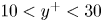 $10< y^+<30$ (Tomkins & Adrian Reference Tomkins and Adrian2003). It can be seen that at relatively low Grashof number (
 $Gr_\delta =1.1\times 10^6$), the normalised premultiplied spectra peaks at
 $\lambda _z^+\approx 600$, whereas at higher Grashof number, the peak shifts inwards to
 $\lambda _z^+ \approx 130$ for both
 $Gr_{\delta } = 6.1\times 10^6$ and
 $Gr_{\delta }=2.7\times 10^7$. This near-wall energetic signature also occurs at fixed wall coordinates (
 $\lambda _z^+\approx 130$ and
 $y^+\approx 15$) for our DNS at high Grashof number, which is seen in figure 7(b) in the temporal development of the spanwise premultiplied spectra at
 $y^+\approx 15$ – as the flow progressively becomes more turbulent, the normalised spanwise spectrum grows in magnitude in this near-wall region, and its peak location agrees with the
 $\lambda _z^+ = 130$ line (grey dashed). A more quantitative representation of the results presented in figure 7(b) can be seen in figure 7(c), where the peak location of the spanwise spectra is plotted against Grashof number. In the present study, the peak location is determined by a wavelength band bounded by
 $90\,\%$ of the instantaneous premultiplied spectra maximum at
 $y^+\approx 15$ (the
 $90\,\%$ boundaries are indicated by the solid lines in figure 7c). As shown in figure 7(c), while the peak wavelength band (i.e. the mean streak spacing) is changing appreciably since the flow becomes turbulent at
 $Gr_{\delta }=10^6$; it attains a constant value at
 $\lambda _z^+\approx 130$, as would have been seen in the fully turbulent flows (Kline et al. Reference Kline, Reynolds, Schraub and Runstadler1967; Patel et al. Reference Patel, Boersma and Pecnik2016) for
 $Gr_{\delta }>6.5\times 10^6$ (see shaded area in figure 7c). Both figures 6 and 7 indicate that the near-wall region is not sufficiently turbulent in the sense of von Kármán at relatively low Grashof number, in which range the NCBL is generally thought turbulent. This constant spacing regime marks the formation of near-wall streaks for the NCBL, and suggests a second stage of the NCBL turbulence development.
Normalised premultiplied spanwise spectra  $k_zE_{uu}/u_\tau ^2$ for the turbulent NCBL at
 $y^+\approx 15$. (a) For different Grashof numbers. (b) Contours of the spanwise spectra
 $k_zE_{uu}/u_\tau ^2$ at
 $y^+\approx 15$ at various
 $Gr_{\delta }$, with coloured vertical lines representing the same information as given in (a). (c) The temporal development of the instantaneous maximum wavelength band, where the upper and lower lines are the boundaries of the region where
 $k_zE_{uu}/u_\tau ^2$ is greater than 90 % of its instantaneous maximum at
 $y^+\approx 15$. The grey dashed line in (b) indicates
 $\lambda _z^+= 130$, and the shaded area in (c) indicates the region
 $Gr_{\delta }>6.5\times 10^6$ and
 $k_zE_{uu}/\max (k_zE_{uu})>90\,\%$.

This near-wall streak evolution is also clearly seen in the wall-parallel planes of the instantaneous velocity contours in the near-wall region. As shown in figures 8(a,b), the instantaneous velocity field at  $y^+\approx 15$ develops increasingly finer structures with increasing
 $Gr_{\delta }$. While the low-speed packets (coloured blue–white in figure 8) occupy a large wall-parallel area for relatively low Grashof number at
 $Gr_{\delta }=1.1\times 10^6$ (cf. Ng et al. Reference Ng, Ooi, Lohse and Chung2017, for non-streaky lower-shear regions), the instantaneous velocity field at
 $Gr_{\delta }=2.7\times 10^7$ appears much more streaky, with streamwise elongated streaks that are commonly seen in the momentum-driven turbulent boundary layers (e.g. Hutchins & Marusic Reference Hutchins and Marusic2007a). Similar observation has been reported by Ng et al. (Reference Ng, Ooi, Lohse and Chung2017) for vertical natural convection in a differentially heated channel. In their analysis, they found that the non-streaky low-speed patches that associate with the low-speed regions decline in size with increasing Grashof number, while the streaky higher-shear regions occupy increasingly larger fractions on the wall areas at higher Grashof number for their steady flows (cf. figures 2 and 3 in Ng et al. Reference Ng, Ooi, Lohse and Chung2017). Figures 8(c,d) show magnified views of the blue boxes in figures 8(a,b), with the horizontal red lines representing the most energetic spanwise wavelengths (
 $\lambda _z^+$ that have the maximum
 $k_zE_{uu}/u_\tau ^2$) indicated by figure 7(a). It is clear that for
 $Gr_{\delta }=1.1\times 10^6$, the most energetic spanwise wavelength
 $\lambda _z^+\approx 600$ agrees well with the spanwise spacing of the low-speed packets (shown in figure 8c), whilst for
 $Gr_{\delta }=2.7\times 10^7$, the most energetic spanwise wavelength
 $\lambda _z^+=130$ in figure 8(d) is representative of the streak spacing (Kline et al. Reference Kline, Reynolds, Schraub and Runstadler1967; Hutchins & Marusic Reference Hutchins and Marusic2007a).
Wall-parallel planes of the normalised instantaneous streamwise velocity  $u/U_s$ in the near-wall region at
 $y^+\approx 15$ for (a)
 $Gr_{\delta }=1.1\times 10^6$, and (b)
 $Gr_{\delta }=2.7\times 10^7$. Here,
 $U_s= (\kappa g \beta \theta _w)^{1/3}$ and
 $L_s=\kappa ^{2/3}/(g\beta \theta _w)^{1/3}$ are the intrinsic velocity and length scales. (c,d) Magnified view of the blue boxes in (a,b), respectively. The horizontal red line in (a) and (c) depicts the most energetic length scale
 $\lambda _z^+ = 600$ at
 $Gr_{\delta }=1.1\times 10^6$; the horizontal red line in (b) and (d) depicts the most energetic length scale
 $\lambda _z^+ = 130$ at
 $Gr_{\delta }=2.7\times 10^7$.

3.3. Identifying the weakly turbulent regime
Although figure 7(c) provides a convenient way to identify the transition from the ‘classical’ turbulent to the fully turbulent regime, in this subsection we present an alternative method to distinguish the ‘classical’ weakly turbulent regime – to show that the identification of this ‘classical’ regime is robust and the transition mechanism is consistent with the near-wall turbulence development discussed in § 3.2.
Previous literature suggests that the transition from the ‘classical’ turbulent regime to the ultimate regime results in a change of the heat transfer rate (e.g. Wells & Worster Reference Wells and Worster2008; Grossmann & Lohse Reference Grossmann and Lohse2011; Ng et al. Reference Ng, Ooi, Lohse and Chung2017). However, as discussed in §§ 3.1 and 3.2, the development of heat transfer and near-wall turbulence structure for the NCBL is gradual, and the transition from the weakly turbulent regime towards the highly turbulent regime is subtle (see also Ke et al. Reference Ke, Williamson, Armfield, Komiya and Norris2021). In the light of the unifying theory (e.g. Grossmann & Lohse Reference Grossmann and Lohse2000, Reference Grossmann and Lohse2011), the near-wall region of the weakly turbulent flow in the ‘classical’ regime would follow a laminar-like scaling (cf. Ng et al. Reference Ng, Ooi, Lohse and Chung2015). Following the Prandtl–Blasius–Pohlhausen scaling (cf. Landau & Lifshitz Reference Landau and Lifshitz1987; Ng et al. Reference Ng, Ooi, Lohse and Chung2015), one would expect the ratio of the wall-normal length scale (usually the boundary layer thickness) to the streamwise length scale (usually the downstream distance for spatially developing flows) to be a function of Reynolds number. However, for the present study, there is no natural length scale in the streamwise direction due to its parallel nature, therefore we adopt a length scale ratio between two wall-normal length scales:
 \begin{equation} \frac{\delta_{u}}{\delta_m} \equiv \frac{\rho \nu \bar{u}_m}{\delta_m \tau_w}. \end{equation}
Here,  $\delta _{u} = {\rho \nu \bar {u}_m}/{\tau _w}$ approximates the thickness of the laminar boundary layer if the flow was laminar up to maximum velocity location
 $\delta _m$. This length scale is also used by Ng et al. (Reference Ng, Ooi, Lohse and Chung2015) to distinguish the boundary-layer-like region from the bulk flow for natural convection in differentially heated channels. Equation (3.5) conveniently distinguishes the length scale development differences in different flow regimes, as shown in figure 9(a). To ease the comparison with non-buoyant flows, the bulk flow Reynolds number
 $Re_m = \delta _m \bar {u}_m /\nu$ is adopted as a measure of the flow development. In the laminar regime, the length scale ratio is given directly by the analytical expression
 \begin{equation} \frac{\delta_{u}}{\delta_m} = \frac{g\beta\theta_w\rho\nu\sqrt{{\rm \pi} }\,\mathcal{V}}{\sqrt{Pr}\,(1-\sqrt{Pr})\,\eta_m} \approx 0.414, \end{equation}
where  $\mathcal {V}= \text {i}^2\text {erfc}(\eta _m)-\text {i}^2\text {erfc}({\eta _m}/{\sqrt {Pr}}) \approx 0.01731$ is a similarity constant at the (laminar) velocity maximum location
 $\eta _m\approx 0.39655$ (cf. Ke et al. Reference Ke, Williamson, Armfield, McBain and Norris2019). The constant
 $\delta _{u}/\delta _m$ in the laminar regime is expected since both
 $\delta _u$ and
 $\delta _m$ are wall-normal length scales and therefore follow the same scaling with the flow development. As seen in figure 9(a), our DNS show excellent agreement with (3.6) in the laminar regime until the flow undergoes laminar–turbulent transition, where
 $\delta _{u}/\delta _m$ starts to decrease. Interestingly, as the flow enters the turbulent regime, a second constant
 $\delta _{u}/\delta _m$ region emerges (for DNS-D this is
 $\delta _u/\delta _m\approx 0.25$) before it reduces again at higher
 $Re_m$ (or, identically,
 $Gr_\delta$). In the present study, we define the limits of this constant region as the
 $Re_m$ at which the length scale ratio exceeds
 $\pm 10\,\%$ of the average value after the flow becomes turbulent, i.e.
 $|{\delta _u/\delta _m - 0.25}| \le 0.025$ and
 $Gr_{\delta }>10^6$ (cf. figure 2, where the Nusselt number starts to follow the empirical
 $1/3$ power law) for DNS-D (indicated by the horizontal grey shading in figure 9). With this criterion, the constant ratio region is identified at
 $290< Re_m<550$ for DNS-D, which corresponds to Grashof number range
 $10^6< Gr_\delta <5\times 10^6$ (indicated by the vertical grey shading in figure 9). This result is consistent with the spanwise turbulence structure development shown in figure 7, where the energetic low-speed packets are seen reduced in strength at approximately
 $Gr_{\delta }\sim 10^6$; and the constant near-wall streak spacing that is commonly seen in fully turbulent flows starts to emerge for NCBL only at
 $Gr_\delta > 6.5\times 10^6$. The existence of such a constant ratio region in the turbulent NCBL at relatively low
 $Re_m$ (or
 $Gr_\delta$) indicates that the near-wall structure of the turbulent flow in this regime may share characteristics and mechanisms similar to those of a laminar flow. Similar constant ratio regions are also seen in the measurements of Tsuji & Nagano (Reference Tsuji and Nagano1988a) for the spatially developing NCBL with
 $\delta _u/\delta _m\approx 0.22$ at similar
 $Re_m$ range, which implies that the measurements of Tsuji & Nagano (Reference Tsuji and Nagano1988a) sit in this ‘classical’ weakly turbulent regime with a turbulent bulk flow and a laminar-like near-wall region, and in DNS-A with
 $\delta _u/\delta _m\approx 0.255$ at approximately
 $320< Re_m<700$ (corresponding to
 $2\times 10^6< Gr_\delta <4\times 10^6$). At higher
 $Re_m$ (or
 $Gr_\delta$), a further decrease is seen in figure 9(a) for DNS-D, which gradually approaches the numerical data in DNS-A and DNS-C with increasing
 $Re_m$, indicating that the flow becomes initial-condition-invariant. In this flow regime, the DNS data for DNS-C also agree well with the measurements of turbulent wall jet flows (Tachie et al. Reference Tachie, Balachandar and Bergstrom2002; Naqavi et al. Reference Naqavi, Tyacke and Tucker2018), suggesting that at high enough
 $Re_m$, the near-wall region would become turbulent in the sense of von Kármán, and appear comparable with the canonical wall-bounded turbulence even though the two flows are driven differently – we will show in the following analysis that this is attributed to the development of the near-wall turbulence.
The length scale ratio development for the NCBL in (a) Reynolds number  $Re_m$ and (b) Grashof number
 $Gr_\delta$, with individual contributions from (3.7) for DNS-D. The grey shaded areas indicate the range of the weakly turbulent regime for DNS-D in
 $290< Re_m<550$ (corresponding to
 $10^6< Gr_\delta <5\times 10^6$) and the region
 $\delta _u/\delta _m = 0.25\pm 0.025$. Open symbols represent the data of DNS-A (blue triangles), DNS-C (red squares) and DNS-D (green diamonds). Filled symbols denote data obtained from other sources: purple circles for experiment measurements of Tsuji & Nagano (Reference Tsuji and Nagano1988a) for a spatially developing NCBL; navy hexagrams for experiment measurements of Tachie, Balachandar & Bergstrom (Reference Tachie, Balachandar and Bergstrom2002) for a wall jet; black stars for DNS data of Naqavi et al. (Reference Naqavi, Tyacke and Tucker2018) for a wall jet. The horizontal black dotted line in (b) indicates the zero line.

To further investigate the near-wall characteristics in this constant-ratio region, the budget of the length scale ratio is obtained by taking the second integral of the mean streamwise momentum equation up to  $\delta _m$ and normalised by a shear forcing
 $\delta _m \tau _w$, which reads
 \begin{align} \frac{\delta_{u}}{\delta_m} &= 1 + \underbrace{ \frac{\rho}{\delta_m\tau_w}\int^{\delta_m}_0\int^{y}_0 \frac{\partial \bar{u}}{\partial t} \,\mathrm{d} y\,\mathrm{d} y }_{\text{TT}} - \underbrace{ \frac{\rho}{\delta_m\tau_w}\int^{\delta_m}_0 \int^{y}_0 g\beta\bar{\theta} \,\mathrm{d} y\,\mathrm{d} y }_{\text{BT}}\nonumber\\ &\quad + \underbrace{\frac{\rho}{\delta_m\tau_w}\int^{\delta_m}_0\overline{u^\prime v^\prime}\,\mathrm{d} y }_{\text{ST}}, \end{align}
where TT, BT and ST denote the temporal (unsteadiness), buoyancy and turbulent shear contributions to the length scale ratio. Ideally, for a steady laminar non-buoyant parallel flow with zero pressure gradient, terms BT, ST and TT are all zero, yielding  ${\delta _u}=\delta _m$ as in the laminar Prandtl–Blasius–Pohlhausen scaling (Landau & Lifshitz Reference Landau and Lifshitz1987). For our NCBL flow, the individual contributions from these terms are depicted in figure 9(b). It is clear that in the laminar regime, ST is zero while BT is mainly responsible for adjusting
 $\delta _u/\delta _m$. When the flow becomes turbulent, both TT and BT appear constant for the entire turbulent regime: TT shows a magnitude (
 $\text {TT}\approx 0.08$) similar to its laminar value, while BT is elevated to
 $\text {BT}\approx 0.85$ from the laminar state (
 $\text {BT}\approx 0.68$). At relatively low
 $Re_m$ in the turbulent regime, the turbulent shear term ST is close to zero (despite its initial decrease at
 $10^6< Gr_{\delta }<2\times 10^6$ due to adjustment from the laminar–turbulent transition) – similar to that of ST in the laminar regime, resulting in a constant
 $\delta _u/\delta _m$ in this regime – whereas at higher
 $Re_m$, ST becoming increasingly negative and therefore
 $\delta _u/\delta _m$ attenuates in the highly turbulent regime. This suggests that the constant
 $\delta _u/\delta _m$ region essentially refers to a turbulent flow regime where the near-wall momentum transfer due to turbulence is negligible (and therefore the ‘weakly turbulent’ or ‘laminar-like’ regime), while a further decrease in
 $\delta _u/\delta _m$ at higher
 $Re_m$ (or
 $Gr_\delta$) is due mainly to the rising strength of the
 $\overline {u^\prime v^\prime }$ stress in the near-wall region (cf. figure 5a), which is also seen strongly in the canonical wall-bounded turbulence (e.g. channel flows and wall jets).
While the length scale ratio (3.5) describes the near-wall turbulence development, it is also directly linked to the skin friction coefficient  $C_f$ for the NCBL flow. By multiplying the bulk Reynolds number
 $Re_m$, (3.5) can be recast into
 \begin{equation} Re_m\,\frac{\delta_u}{\delta_m} = \frac{\rho \bar{u}_m^2}{\tau_w} = \frac{2}{C_f} . \end{equation}
From (3.8), a constant  $\delta _u/\delta _m$ that is seen in the laminar and weakly turbulent regimes would lead to
 $C_f \propto Re_m^{-1}$, as shown in figure 10, which is consistent with the skin friction correlation for Blasius boundary layers (with different prefactors). Note that the second equality of (3.8) can be rewritten as
 $C_f = {2}/{(u^+_m)^2}$, such that the skin friction coefficient can also be approximated by the velocity log law (which starts to appear only at sufficiently high
 $Re_m$, or equivalently,
 $Gr_\delta$) based on the maximum mean streamwise velocity
 $u^+_m$ in wall units. Although the formulation of the buoyancy-modified velocity log law (cf. Ke et al. Reference Ke, Williamson, Armfield, Norris and Komiya2020, equation (6.29)) relies on the buffer layer velocity
 $u_c$ for which we have no model, in the present study we are able to apply the log-law approximation by fitting empirically
 $u_c$ from DNS data. Despite the fact that the velocity maximum usually occurs beyond the extent of the log-law region, for high
 $Re_m$, flows the log-law approximation still demonstrates good agreement with the DNS data, as shown in figure 10. In this regime, the skin friction coefficient
 $C_f$ also agrees well with a simplified approximation
 \begin{equation} C_f = \frac{2D^2}{\ln^2(0.06\,Re_m)}, \end{equation}
where  $D=0.31$ is a empirical prefactor associated with the mixing length coefficient (cf. the mixing length coefficient in the buoyancy modified log law in Ke et al. Reference Ke, Williamson, Armfield, Norris and Komiya2020) for our NCBL. This approximation (3.9) takes a similar form to the wall friction expression for the turbulent boundary layers (cf. Kestin & Persen Reference Kestin and Persen1962; White Reference White1991;
 $C_f = 2D^2/\ln ^2(0.06\,Re_x)$, with
 $D=0.477$). With reference to figure 10, it further supports the idea that the turbulent NCBL has two distinct regimes: at relatively low
 $Re_m$, it follows
 $C_f\propto Re_m^{-1}$, representing a ‘laminar-like’ near-wall region, while at large
 $Re_m$, a log-law-type scaling is seen, which is indicative of a fully turbulent flow in the sense of von Kármán being developed.
The skin friction coefficient  $C_f$ for the NCBL. The red dotted line indicates the skin friction coefficient for the laminar Blasius boundary layer (Reynolds number based on the disturbance thickness); black dotted lines correspond to the skin friction coefficient for the laminar regime
 $C_f = (2/0.414)\,Re_m^{-1}$ and the weakly turbulent regime
 $C_f = (2/0.25)\,Re_m^{-1}$ based on (3.8); orange crosses are the approximation of
 $C_f$ by empirically fitting
 $u_c$ to the log-law model (for clarity, not all data are shown); the yellow dotted line is indicative of the simplified approximation (3.9).

3.4. Turbulence kinetic energy budget
In this subsection, we explore how the turbulence in the near-wall region is produced and sustained by examining the turbulence kinetic energy budget. The energetic balance has been crucial in explaining the flow regimes and obtaining Nusselt number scaling relationships in canonical flows – for example, Rayleigh–Bénard flow (Grossmann & Lohse Reference Grossmann and Lohse2000, Reference Grossmann and Lohse2001, Reference Grossmann and Lohse2011) and differentially heated channel flow (Ng et al. Reference Ng, Ooi, Lohse and Chung2018). Such information will lead to a better understanding of the turbulence mechanisms in the near-wall region, which may aid the development of scaling relationships for turbulence models.
For our temporally developing parallel flow ( $\bar {v}=\partial \bar {\psi }/\partial x = \partial \bar {\psi }/\partial z=0$, where
 $\psi$ is an arbitrary flow variable of interest – note that for our temporally developing flow, the statistics are averaged spatially over the homogeneous
 $x$–
 $z$ plane), the equation for the turbulence kinetic energy reads
 \begin{equation} \frac{\partial \bar{k}}{\partial t} = P+T_t+T_p+D_f+\varepsilon+\mathcal{B}, \end{equation}
where  $\bar {k}=\overline {{u^\prime }_i^2}/2$ is the turbulence kinetic energy,
 $P$ represents the shear production,
 $T_t$ is the turbulent convection,
 $T_p$ is the pressure transport,
 $D_f$ is the viscous diffusion,
 $\varepsilon$ denotes the viscous dissipation, and
 $\mathcal {B}$ is the buoyancy flux term. The individual contributions from production, dissipation and transport terms towards the temporal evolution of the turbulence kinetic energy are given by
 \begin{gather} P ={-}\overline{u^\prime v^\prime}\,\frac{\partial \bar{u}}{\partial y}, \quad T_t ={-}\frac{\partial \overline{v^\prime k}}{\partial y} ,\quad T_p ={-}\frac{1}{\rho}\,\frac{\partial \overline{v^\prime p^\prime } }{\partial y}, \end{gather}
 \begin{gather}D_f =\nu\,\frac{\partial ^2 \bar{k} }{\partial y^2},\quad \varepsilon ={-}\nu\,\overline{\left(\frac{\partial u^\prime_i}{\partial x_j }\right)^2},\quad \mathcal{B} = g\beta\,\overline{u^\prime\theta^\prime}. \end{gather}
Figure 11 shows the contributors in (3.11) to the turbulence kinetic energy in the ‘classical’ regime (figure 11a) and the fully turbulent ultimate regime (figures 11b–figure 11a). As shown in figure 11(a), there exist two local peaks for the shear production  $P$. Such a structure is typical in flows with two shear layers under similar general flow geometries (e.g. the planar wall jet flows; Naqavi et al. Reference Naqavi, Tyacke and Tucker2018; Gnanamanickam et al. Reference Gnanamanickam, Bhatt, Artham and Zhang2019) as these are the signature of the energetic mixing in the shear layers. For our NCBL flow, the shear production
 $P$ has an inner local peak at
 $y^+\approx 10$, which corresponds to the near-wall shear layer as would have been seen in the canonical boundary layer flows, and an outer peak at
 $y/\delta _m\approx 4$, which corresponds to the free shear layer in the bulk flow. Although the near-wall turbulent shear
 $\overline {u^\prime v^\prime }$ is negligible in the ‘classical’ regime (see figure 5a), as seen in figure 11(a), the inner peak of the shear production still shows a similar magnitude to the outer peak. However, the buoyancy flux term is shown to have only minimal effect (with slightly negative values) in this region – the primary role of buoyancy is to accelerate the mean flow (see Ke et al. Reference Ke, Williamson, Armfield, Norris and Komiya2020), which generates turbulence via shear production, rather than direct buoyant production of turbulence. It can be seen that in addition to the shear production, the near-wall turbulence at this stage is transported predominantly from the outer bulk flow by pressure
 $T_p$. The net gain of the turbulence kinetic energy is balanced by the viscous dissipation (and diffusion for
 $y^+>5$), while turbulent transport is rather weak since the near-wall flow is laminar-like with small turbulent fluctuation intensity. Away from the wall, the buoyancy flux term contributes positively to the turbulence generation in the bulk flow over a large distance (
 $0.2< y/\delta _m<10$ for DNS-D at
 $Gr_{\delta }=1.1\times 10^6$ with peak
 $\mathcal {B}\nu /u_\tau ^4 \approx 0.01$) due to the excursion of warmer fluid parcels from the near-wall region (recall in figure 5(a),
 $\overline {u^\prime v^\prime }$ is positive in the bulk flow region). In the free shear layer (
 $y/\delta _m>1$), shear production
 $P$, being the dominant term driving turbulence, is balanced mainly by dissipation – with the excess energy being transported towards the edge of the flow as well as the maximum velocity location. This suggests that the outer bulk flow has indirect influence on the near-wall region by adjusting the energetic behaviour at
 $y\sim \delta _m$. Similar transport effects on the near-wall turbulence are also seen in planar wall jets (Naqavi et al. Reference Naqavi, Tyacke and Tucker2018), where turbulence in the low-production region (which is also identified as the interaction zone of two shear layers) is typically maintained by a high level of turbulent transportation.
The turbulence kinetic energy budget of the temporally developing NCBL at (a) DNS-D,  $Gr_\delta =1.1\times 10^6$ (
 $Re_\tau \approx 34$), and (b) DNS-D,
 $Gr_\delta =2.7\times 10^7$ (
 $Re_\tau \approx 85$). (c) Magnified view of the data shown in (b) in the near-wall region. (d) The near-wall region of DNS-A at
 $Gr_{\delta }=4.1\times 10^7$ (
 $Re_\tau \approx 117$). All terms are normalised into wall units with
 $\bar {u}_m^3/\delta _m$ (left-hand axis) and
 $u_\tau ^4/\nu$ (right-hand axis) in (a,b), while data in (c,d) are shown in wall units. Lines denote the DNS results from DNS-A and DNS-D; symbols in (c,d) denote the DNS data in wall coordinate taken from Kasagi & Nishimura (Reference Kasagi and Nishimura1997) for a combined convection in a differentially heated channel with aiding ambient flow at
 $Re_\tau = 86$. Colours represent individual components of the turbulence kinetic energy budget: red for shear production; blue for viscous dissipation; magenta for viscous diffusion; green for turbulent convection; lilac for pressure transport; orange for buoyancy production. Black dotted lines mark the zero line.

At higher  $Gr_\delta$, the flow enters the fully turbulent regime as shown in figure 11(b); the near-wall shear production grows in strength and becomes dominant in this region (at
 $Gr_{\delta }=2.7\times 10^7$ it is approximately four times larger than the outer peak); and the buoyancy flux term remains negligible in the near-wall region and shrinks in magnitude (with peak
 $\mathcal {B}\nu /u_\tau ^4\approx 0.004$) in the outer bulk flow. While both turbulent and pressure transport terms are following behaviour similar to the weakly turbulent case in figure 11(a), it gives a higher level of turbulent transport and a lower level of pressure transport in the near-wall region as the flow becomes more turbulent. Figure 11(c) shows a magnified view of these contributors at
 $Gr_{\delta }=2.7\times 10^7$ in the near-wall region, and compares with the DNS data taken from Kasagi & Nishimura (Reference Kasagi and Nishimura1997) for a combined convection in a differentially heated channel with aiding ambient flow at
 $Re_\tau =86$ (based on
 $\delta _m$). It can be seen that despite the close
 $Re_\tau$ reported, the data of Kasagi & Nishimura (Reference Kasagi and Nishimura1997) show a higher level of production, dissipation and turbulent transport, and a lower level of pressure effect in the vicinity of the wall (
 $y^+<60$) than our DNS-D at
 $Re_\tau \approx 85$. Such a discrepancy is not surprising as the combined convection has a more energetic flow in the near-wall region with the aid of ambient momentum (cf. Kasagi & Nishimura (Reference Kasagi and Nishimura1997) for the near-wall shear stress), resulting a higher level of shear and a more turbulent flow in the near-wall region. This is supported by the fact that their data appear more comparable to our temporal NCBL at a much higher Grashof number: as shown in figure 11(d), our DNS-A at
 $Re_\tau \approx 117$ (
 $Gr_{\delta }=4.1\times 10^7$ in the fully turbulent regime) demonstrates relatively good quantitative agreement with the combined convection at
 $Re_\tau =86$ (again we note that
 $Re_\tau$ alone does not fully characterise the NCBL flow since the buoyancy effects are not accounted for).
The sum of the right-hand-side terms in (3.11), giving the temporal growth of the turbulence kinetic energy, is shown in figure 12. We note that this temporal evolution rate is more than an order of magnitude smaller than the contributors shown in figure 11. Despite the strong oscillations due to the small magnitude and the temporal nature of the turbulence flow, figure 12 still shows a clear signature of the turbulence energy evolution for the NCBL: for all data shown, the temporal growth of turbulence occurs predominantly in the outer bulk flow (i.e. the free shear layer) with a distributed peak at  $y/\delta _m\approx 10$. At
 $Gr_\delta = 1.1\times 10^6$, the turbulence energy experiences a weak decay (negative growth rate) in the near-wall region
 $y/\delta _m< O(1)$. With increasing Grashof number, owing to a growing local production at
 $y/\delta _m\approx 0.1$ (cf. figure 11b), the turbulence growth rate attains a positive value and spreads to a wider area towards the near-wall region, giving rise to a net local turbulence energy gain in the near-wall region.
The temporal evolution of the turbulence kinetic energy (normalised with the outer bulk scales  $\delta _m$ and
 $\bar {u}_m$) for the NCBL at different Grashof numbers. The horizontal dotted line indicates
 $\partial k/\partial t =0$.

Figure 13 shows the production–dissipation equilibrium for the temporally developing NCBL flow in wall coordinate (figure 13a) and the outer bulk scale  $\delta _m$ (figure 13b). Also shown in figure 13 are the DNS results of a combined convection at
 $Re_\tau =86$ (Kasagi & Nishimura Reference Kasagi and Nishimura1997), a turbulent channel flow at
 $Re_\tau =180$ (Moser et al. Reference Moser, Kim and Mansour1999;
 $Re_\tau$ based on the channel half-width), and a planar wall jet at
 $Re_\tau =210$ (Gnanamanickam et al. Reference Gnanamanickam, Bhatt, Artham and Zhang2019;
 $Re_\tau$ based on
 $\delta _m$). This ratio of shear production to viscous dissipation
 $P/\varepsilon$ evaluates the balance between local production and destruction of the turbulent energy, and is a key parameter that characterises the logarithmic layer for canonical wall-bounded forced flows. In the near-wall region, as depicted in figure 13(a),
 $P/\varepsilon$ increases with increasing
 $Gr_{\delta }$ since the shear becomes progressively stronger with the development of the flow: at
 $Gr_{\delta }=1.1\times 10^6$, dissipation exceeds production,
 $P/\varepsilon <1$, suggesting that the near-wall turbulence is sustained with the transportation of energy from regions away from the wall; at higher
 $Gr_{\delta }$, production exceeds dissipation, and the
 $P/\varepsilon$ profile is more comparable to the forced flows reported by Kasagi & Nishimura (Reference Kasagi and Nishimura1997) and Moser et al. (Reference Moser, Kim and Mansour1999) for
 $y^+<30$. Beyond
 $y^+=30$, the production and dissipation are almost in balance (such that
 $P/\varepsilon \approx 1$) for the channel flow in the log-law region (
 $30< y+< O(10^2)$), whereas such a plateau is absent for our NCBL. The balanced production and dissipation (i.e.
 $P/\varepsilon \approx 1$) is often observed in the logarithmic layer for the canonical forced wall-bounded flows, and it has been seen as a prerequisite to obtain a valid mixing length model for the log-law region (Pope Reference Pope2001). For our vertical NCBL flow, it is shown in figure 13 that the production–dissipation ratio
 $P/\varepsilon$ follows a fundamentally different profile in the log-law region – despite the absence of the canonical
 $P/\varepsilon$ prerequisite for the log-law, the NCBL flow can still be very well modelled by the mixing length model with a buoyancy-adjusted log-law (cf. Ke et al. Reference Ke, Williamson, Armfield, Norris and Komiya2020). Similar
 $P/\varepsilon$ behaviour in this region is also seen in the combined convection in a differentially heated channel (Kasagi & Nishimura Reference Kasagi and Nishimura1997) and the planar wall jet (Gnanamanickam et al. Reference Gnanamanickam, Bhatt, Artham and Zhang2019), which is suggestive that the missing equilibrium here might due to the interaction of shear layers since the production is forced to zero at
 $y=\delta _m$ with
 $\partial \bar {u}/\partial y = 0$. In the region
 $0.6< y/\delta _m<1$ (see figure 13b),
 $P/\varepsilon$ of our NCBL flow decays quickly to its minimum, which is slightly negative. The lack of production suggests a high level of transport from the neighbouring shear layers in order to preserve turbulence in this region (cf. figure 11, high level of turbulent transport in this region). This is consistent with the observation of the planar wall jet flows that
 $P/\varepsilon$ is either very small or negative in the interaction zone (Irwin Reference Irwin1973; Zhou, Heine & Wygnanski Reference Zhou, Heine and Wygnanski1996; Dejoan & Leschziner Reference Dejoan and Leschziner2005). This interaction zone for our temporally developing NCBL is seen to decline in size with increasing
 $Gr_{\delta }$. Farther away in the bulk region (
 $y/\delta _m>1$, see figure 13b), a high level of production is observed for our NCBL flow. In this region, the shear production is typically associated with the temporal growth of the boundary layer thickness due to entrainment (cf. Ke et al. Reference Ke, Williamson, Armfield, Komiya and Norris2021; the entrainment coefficient is dominated by the total shear production in the bulk region). Meanwhile, the production–dissipation ratio is approximately constant at
 $P/\varepsilon \approx 1.5$ regardless of
 $Gr_{\delta }$, while for the planar wall jet (Gnanamanickam et al. Reference Gnanamanickam, Bhatt, Artham and Zhang2019), the production is in equilibrium with the dissipation, giving a unity
 $P/\varepsilon$ in the free shear layer. This value is close to that of the homogeneous shear flows with uniform mean velocity gradient (e.g. Tavoularis & Corrsin Reference Tavoularis and Corrsin1981; Rogers & Moin Reference Rogers and Moin1987; De Souza, Nguyen & Tavoularis Reference De Souza, Nguyen and Tavoularis1995; giving
 $P/\varepsilon \approx 1.4\sim 1.7$) in which the transport process is absent and the excess energy completely contributes to the exponential growth of the turbulence in time. However, in our temporally developing NCBL, the excessive energy generated by shear is mostly transported towards the interaction zone by turbulent transport (cf. figure 11,
 $T_t$ is about half of
 $\varepsilon$), which implicitly affects the near-wall turbulence by adjusting the turbulence balance in this low-production region, while the remainder contributes to the temporal growth of the turbulence.
Production–dissipation ratio in the near-wall region (a) in wall coordinate and (b) normalised by the bulk flow length scale  $\delta _m$. The arrow in (a) shows the direction of increasing
 $Gr_{\delta }$ for cases with buoyancy. Horizontal dotted lines in (a,b) indicate
 $P/\varepsilon =0$,
 $1$ and
 $1.5$.

4. Conclusions
In this paper, a vertical natural convection boundary layer (NCBL) with  $Pr=0.71$ has been investigated using direct numerical simulations (DNS) in a temporal framework. Previous studies have suggested that there is a change in the heat transfer rate for turbulent NCBLs from a ‘classical’
 $1/3$ power law to a higher ultimate heat transfer (Grossmann & Lohse Reference Grossmann and Lohse2000; Ng et al. Reference Ng, Ooi, Lohse and Chung2017) at large Grashof number. While such a transition in the turbulent heat transfer is expected, this process has been shown to develop very slowly and subtly over a very large range of Grashof number (Wells & Worster Reference Wells and Worster2008; Ng et al. Reference Ng, Ooi, Lohse and Chung2017; Ke et al. Reference Ke, Williamson, Armfield, Komiya and Norris2021), and as such, it is difficult to discern the regime change in the turbulence development. In the present study, clear evidence is presented showing the presence of a regime where the outer bulk flow is turbulent but in which the near-wall region is predominantly laminar, consistent with the development for canonical wall-bounded turbulence (Kraichnan Reference Kraichnan1962; Grossmann & Lohse Reference Grossmann and Lohse2000).
Turbulent statistics, momentum balance and the development of energy spectra support this conclusion. We show that the Reynolds shear stress has a close-to-zero negative trough in the near-wall region after laminar–turbulent transition since the near-wall momentum transfer due to turbulence mixing is weak in the ‘classical’ regime, which is consistent with the existing measurements (Tsuji & Nagano Reference Tsuji and Nagano1988a; Abedin et al. Reference Abedin, Tsuji and Hattori2009; Nakao et al. Reference Nakao, Hattori and Suto2017). With increasing Grashof number, the negative trough becomes larger in magnitude as the turbulent momentum transfer grows in strength. A similar trend has been seen strongly in canonical wall-bounded turbulence (e.g. Moser et al. Reference Moser, Kim and Mansour1999) and buoyancy-driven channel flows (e.g. Kim et al. Reference Kim, Ahn and Choi2021). Further evidence may be seen in the streamwise turbulence intensity development, where it develops gradually from a mono-peak profile into a dual-peak structure. Using premultiplied power spectra of the streamwise velocity fluctuation, we show that the growing inner peak of the  $\overline {u^\prime u^\prime }$ stress is located at a fixed location and wavelength (
 $y^+=18$ and
 $\lambda _x^+=1000$) in the viscous coordinate, similar to that in canonical wall-bounded turbulence (Del Alamo et al. Reference Del Alamo, Jiménez, Zandonade and Moser2004; Hutchins & Marusic Reference Hutchins and Marusic2007b). In contrast to the forced flows where the outer energetic peak, which accounts for the logarithmic region for these flows, becomes visible only at sufficiently high Reynolds number and after the inner peak has been developed, the emerging inner peak in our DNS data suggests that the NCBL follows a different turbulence development. Further evidence is also seen in the spanwise premultiplied spectra, which are representative of the near-wall streak spacing in the fully turbulent regime. It is shown that the mean streak spacing varies appreciably with
 $Gr_{\delta }$ at relatively low Grashof number (
 $10^6< Gr_{\delta }< 6.5\times 10^6$; in this regime, the NCBL is generally thought turbulent in the literature), while at higher
 $Gr_{\delta }$, it is approximately constant,
 $\lambda _z^+ \approx 130$. Such a constant spacing marks the formation of the turbulent near-wall streaks that is commonly seen in fully turbulent wall-bounded flows (Kline et al. Reference Kline, Reynolds, Schraub and Runstadler1967; Klewicki et al. Reference Klewicki, Metzger, Kelner and Thurlow1995; Tomkins & Adrian Reference Tomkins and Adrian2003; Patel et al. Reference Patel, Boersma and Pecnik2016), which is suggestive of a second stage of the turbulence development.
Following the Prandtl–Blasius–Pohlhausen scaling (Landau & Lifshitz Reference Landau and Lifshitz1987; Ng et al. Reference Ng, Ooi, Lohse and Chung2015), we identified the weakly turbulent ‘classical’ regime in which the length scale ratio  $\delta _u/\delta _m$ is a constant. By comparing our DNS with previous datasets, this ‘classical’ regime is found to span approximately
 $250< Re_m<550$ for both DNS-D and the measurements of Tsuji & Nagano (Reference Tsuji and Nagano1988a). This Reynolds number range is equivalent to
 $10^6< Gr_{\delta }<5\times 10^6$ for DNS-D, which appears consistent with the development of the near-wall streaks. On further analysis, we show that such a constant
 $\delta _u/\delta _m$ is indeed attributed to a negligible near-wall turbulence in this Reynolds number range. In this regime, the skin friction coefficient
 $C_f$ is shown to follow a laminar-like scaling with the bulk Reynolds number. At higher
 $Re_m$ (or
 $Gr_{\delta }$), a log-law-type scaling is seen for
 $C_f$, which further supports that the near-wall region has been developed into a fully turbulent one.
To provide a more complete view of the near-wall turbulence generation and development, we further investigated the energetic contributors to the turbulence kinetic energy balance. For the NCBL, there exist two local peaks for the shear production, corresponding to the two shear layers in the flow. At  $Gr_{\delta }=1.1\times 10^6$, the near-wall peak of the shear production has magnitude similar to its outer counterpart, and the turbulent transport is small since the flow is weakly turbulent in the ‘classical’ regime. The near-wall turbulence at this stage is sustained predominantly by the pressure transport in addition to the shear production. With increasing
 $Gr_{\delta }$, the flow enters the fully turbulent regime, and both turbulent transport and shear production grow in magnitude while the pressure transport gradually loses its significance. We show that the buoyancy flux term is negligibly small in the near-wall region with negative values, while it contributes positively to the turbulence generation in the bulk flow. These results suggest that the NCBL develops in a way such that the near-wall turbulence is driven by the turbulent outer bulk until it is sufficiently large that turbulence can be generated and sustained locally. Upon further investigation, we show that the production–dissipation balance of our NCBL follows a fundamentally different profile to that of the canonical wall-bounded turbulence where an equilibrium
 $P/\varepsilon =1$ is expected in the log-law region, and such a discrepancy may be attributed to the interaction between the shear layers. While
 $P/\varepsilon$ grows in magnitude with increasing
 $Gr_{\delta }$ in the near-wall region, it remains at an approximately constant value across the outer bulk flow, with
 $P/\varepsilon \approx 1.5$ regardless of
 $Gr_{\delta }$. The excessive energy in the bulk region is transported to the velocity maximum location (the low-production region where the two shear layers interact) by turbulent transport and therefore affects the near-wall turbulence generation.
These results have implications for a better understanding of the near-wall turbulence mechanisms for NCBL flows, which may aid the development of scaling relationships for turbulence models.
Acknowledgements
The authors gratefully acknowledge the computational resources provided by the Institute of Fluid Science, Tohoku University, and by the Sydney Informatics Hub, University of Sydney.
Declaration of interests
The authors report no conflict of interest.


 Open access

