2.1 Governing equations

We consider an incompressible binary mixing of two species of density $\unicode[STIX]{x1D70C}_{1}$ and $\unicode[STIX]{x1D70C}_{2}$ respectively, with $\unicode[STIX]{x1D70C}_{2}>\unicode[STIX]{x1D70C}_{1}$ . We denote respectively $\ell _{0}$ , $u_{0}$ and $\unicode[STIX]{x1D70C}_{0}=(\unicode[STIX]{x1D70C}_{1}+\unicode[STIX]{x1D70C}_{2})/2$ the characteristic length, velocity and density scales. In the limit of zero Mach number, the equation of state can be combined with both the continuity equation and the transport equation of the mass fraction of one of the species to show that the non-solenoidal part of the velocity field is of a diffusive nature (Joseph Reference Joseph1990; Sandoval Reference Sandoval1995),

where $\mathit{Re}=(u_{0}\ell _{0}\unicode[STIX]{x1D70C}_{0})/\unicode[STIX]{x1D707}$ and $\mathit{Sc}=\unicode[STIX]{x1D707}/\unicode[STIX]{x1D70C}_{0}\mathscr{D}$ are the Reynolds and Schmidt numbers with $\unicode[STIX]{x1D707}$ the dynamic viscosity of the mixing and $\mathscr{D}$ the Fickian diffusivity of one of the species into the other. We consider $\unicode[STIX]{x1D707}$ and $\mathscr{D}$ to be constant, which is a fair approximation for a binary mixing of perfect gases, see Fontane (Reference Fontane2005) for the specific case of the air–helium couple. The relevant parameter of the inertia effect is the Froude number $\mathit{Fr}=u_{0}/\sqrt{g\ell _{0}\mathit{ At}}$ in which the Atwood number is defined by $\mathit{At}=\unicode[STIX]{x0394}\unicode[STIX]{x1D70C}/\unicode[STIX]{x1D70C}_{0}$ where $\unicode[STIX]{x0394}\unicode[STIX]{x1D70C}=(\unicode[STIX]{x1D70C}_{2}-\unicode[STIX]{x1D70C}_{1})/2$ is the scale for the density difference. As we address buoyancy-free flows, the Froude number is assumed to be large, i.e. $\mathit{Fr}\gg 1$ , and the dimensionless Navier–Stokes equations read

where $D_{t}=\unicode[STIX]{x2202}_{t}+(\boldsymbol{u}\boldsymbol{\cdot }\unicode[STIX]{x1D735})$ stands for the material derivative. The corresponding vorticity equation is obtained by taking the curl of the momentum equation (2.3)

where the third term on the right-hand side is the baroclinic torque $\boldsymbol{b}=(1/\unicode[STIX]{x1D70C})\unicode[STIX]{x1D735}\unicode[STIX]{x1D70C}\times (1/\unicode[STIX]{x1D70C})\unicode[STIX]{x1D735}p$ which becomes active for misaligned isopycnals and isobars. It is responsible for the specific features of the variable-density flows considered here and will be of central interest in the following. In the inviscid limit, it can be rewritten as the cross-product between the acceleration of the flow itself $\boldsymbol{a}=D_{t}\boldsymbol{u}=-(1/\unicode[STIX]{x1D70C})\unicode[STIX]{x1D735}p$ and the density gradient

which stresses the particular nature of the baroclinic vorticity production considered here compared to stratified geophysical flows where the flow acceleration is replaced by the gravity acceleration $\boldsymbol{g}$ .

2.2 The time-dependent VDKH roll-ups

The two-dimensional base flow consists of a time-evolving shear layer between two fluids of different density which undergoes the development of a KH instability biased by the density contrast. It is obtained through direct numerical simulations using a two-dimensional dealiased pseudo-spectral method described in detail in Joly, Fontane & Chassaing (Reference Joly, Fontane and Chassaing2005) and Joly & Reinaud (Reference Joly and Reinaud2007). The $x$ and $y$ axes correspond to the longitudinal and crosswise directions. The spanwise direction along the $z$ -axis will only serve for the subsequent non-modal stability analysis. Since co-gradient and counter-gradient variable-density mixing layers are equivalent in the frame of temporal approximation at infinite Froude number (Fontane & Joly Reference Fontane and Joly2008), we arbitrarily choose a co-gradient mixing layer by placing the lighter fluid in the lower part of the flow. We take $u_{0}$ as half the velocity difference across the shear layer and $\ell _{0}$ as half the vorticity thickness of the shear layer as characteristics velocity and length scales. The normalised profiles of velocity $\overline{\boldsymbol{U}}=(\overline{U}_{x},0)$ and density $\overline{R}$ of the initial variable-density parallel shear flow are:

This flow is perturbed by the most unstable mode of the inviscid temporal linear stability analysis as described in Fontane & Joly (Reference Fontane and Joly2008). Its amplitude is prescribed such that the enstrophy of the perturbation is a small fraction of the enstrophy of the parallel shear layer over a period. The value $a_{KH}$ of this fraction is set so that the primary KH instability saturates at $t_{KH}=30$ . The two-dimensional velocity $\boldsymbol{U}=(U_{x},U_{y})$ and density $R$ fields are calculated on the domain $[0,L_{x}]\times [-L_{x}/2,L_{x}/2]$ . The initial thickness of the shear layer is set so that the most amplified KH mode corresponds to a wavenumber of $2\unicode[STIX]{x03C0}/L_{x}$ . The boundary conditions are periodic in the longitudinal direction while a free-slip boundary condition is imposed in the crosswise direction. The vertical extent of the domain is large enough so that the free-slip wall do not strongly affect the nonlinear development of the flow (Fontane & Joly Reference Fontane and Joly2008). We focus specifically on the influence of density effects on the development of secondary instabilities and we vary the Atwood number while both Reynolds and Schmidt numbers are fixed to $\mathit{Re}=1000$ and $\mathit{Sc}=1$ . The same value of the Reynolds number has been used in the work of Arratia et al. (Reference Arratia, Caulfield and Chomaz2013) to which we compare our results. It is also representative of the values for which side jets naturally arise in light jets (Monkewitz & Pfizenmaier Reference Monkewitz and Pfizenmaier1991; Fontane Reference Fontane2005). 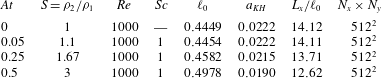For all simulations, we use a mesh of $512^{2}$ points, which has been checked to be large enough to ensure convergence of the results. Note that the number of points used here is far smaller than the ones used by Fontane & Joly (Reference Fontane and Joly2008) in the infinite Schmidt number case where the absence of mass diffusion induces the need for a constantly growing spatial resolution. All these numerical settings are summarised in table 1.

Table 1.

Main numerical parameters for the four simulated VDKH base-flow fields: Atwood number $\mathit{At}$ , density ratio $S=\unicode[STIX]{x1D70C}_{2}/\unicode[STIX]{x1D70C}_{1}$ , Reynolds number $\mathit{Re}$ , Schmidt number $\mathit{Sc}$ , half the initial vorticity thickness $\ell _{0}$ , fraction $a_{KH}$ of the initial enstrophy of the KH mode relative to the enstrophy of the parallel shear layer, ratio $L_{x}/\ell _{0}$ between the domain size and half the initial vorticity thickness, mesh size $N_{x}\times N_{y}$ .

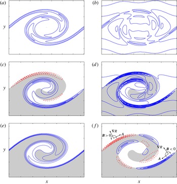
As will be confirmed later in § 3, the inner roll-up structure has a strong influence on the characteristics of the secondary perturbations. Hence, we now briefly describe the specific feature of the VDKH billow compared to the classic homogeneous KH roll-up. Figures 1(a) and 1(c) display the vorticity field at saturation time $t_{KH}=30$ for the homogeneous case $\mathit{At}=0$ and the most density-contrasted case $\mathit{At}=0.5$ . In the later, not only the vorticity field has lost its symmetry but it also concentrates into two sheets of opposite sign on either side of the braid saddle point. This reorganisation of the vorticity field is the consequence of the baroclinic multi-polar source–sink system advocated by Soteriou & Ghoniem (Reference Soteriou and Ghoniem1995) and Reinaud et al. (Reference Reinaud, Joly and Chassaing2000) and illustrated in figure 1(f). In this figure, we represent the acceleration and density gradient near the two main source and sink patches in order to illustrate the local contribution of the baroclinic torque according to its inviscid approximation (2.5). The baroclinic vorticity production induces also a slight asymmetry in the density field which results in a preferential entrainment of the light fluid towards the heavy flow as seen in figure 1(e). Another consequence of the baroclinic vorticity redistribution lies in a drastic change in the strain field. Following Caulfield & Kerswell (Reference Caulfield and Kerswell2000), the strain field $\unicode[STIX]{x1D716}$ of the base flow defined as

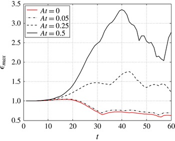
is plotted at $t_{KH}$ in figures 1(b) and 1(d) for the homogeneous case and the most density-contrasted case respectively. The evolution of its structure follows the reorganisation of the vorticity field: it is progressively concentrated and intensified within the two vorticity-enhanced layers on either side of the braid hyperbolic point as the Atwood number is increased. The levels of strain reached there are significantly higher than in the homogeneous case. This is confirmed in figure 2 where the evolution of the maximum strain rate is plotted for the four Atwood numbers considered. While the maximum strain rate is decreasing in the homogeneous case after $t=20$ , it is increasing for large Atwood number. At saturation of the primary KH instability, the measured value is three times higher for $\mathit{At}=0.5$ than in the homogeneous case.

Compared to its homogeneous counterpart, the VDKH billow exhibits an asymmetric layered vorticity field holding much higher levels of strain. Vorticity being generated on thin layers associated with length scales smaller than the ones found in the smooth homogeneous base flow, an increase in Atwood number is likely to promote energy growth for larger spanwise wavenumbers.

Figure 1.

Base-flow characteristics at the saturation time $t_{KH}=30$ : (a) spanwise vorticity field for $\mathit{At}=0$ , (b) strain field for $\mathit{At}=0$ , (c) spanwise vorticity field for $\mathit{At}=0.5$ , (d) strain field for $\mathit{At}=0.5$ , (e) density field for $\mathit{At}=0.5$ and (f) spanwise baroclinic torque for $\mathit{At}=0.5$ . In figures (c)–(f), the grey-shaded region corresponds to the domain where the base-flow density is lower than $\unicode[STIX]{x1D70C}_{0}$ and dashed contours correspond to positive values. In all figures, tick marks along $x$ and $y$ axis are separated by the initial vorticity thickness $\unicode[STIX]{x1D6FF}_{\unicode[STIX]{x1D714}}^{0}=2l_{0}$ . These conventions will hold throughout the paper.

Figure 2.

Influence of the Atwood number on the temporal evolution of the maximum value $\unicode[STIX]{x1D716}_{max}$ of the base-flow strain rate normalised by its initial value.

2.3 Optimisation problem

We now consider the linear evolution of three-dimensional perturbations $[\boldsymbol{u},\unicode[STIX]{x1D70C},p]$ that are likely to develop on top of the VDKH billows $[\boldsymbol{U},R,P]$ . We linearise the governing equations (2.1)–(2.3) around the two-dimensional base flow:

where $D=\unicode[STIX]{x1D735}\boldsymbol{\cdot }\boldsymbol{U}$ and $d=\unicode[STIX]{x1D735}\boldsymbol{\cdot }\boldsymbol{u}$ . This linear system – referred to as the direct system – can be cast in the following compact form:

where $\boldsymbol{q}=[\boldsymbol{u},\unicode[STIX]{x1D70C},p]$ and the three matrix operators are respectively the temporal operator $\unicode[STIX]{x1D649}_{t}$ , the operator of coupling between the base flow and the perturbation $\unicode[STIX]{x1D649}_{c}$ and the diffusion operator $\unicode[STIX]{x1D649}_{d}$ . Their expressions are detailed in appendix A.

In the frame of non-modal stability analysis, the temporal behaviour is not prescribed, and taking into account the streamwise periodicity and the spanwise homogeneity of the base flow, the perturbations are sought under the form

where $k$ is the real spanwise wavenumber and $\unicode[STIX]{x1D707}\in [0,1]$ the real Floquet exponent. Note that the spanwise velocity component is phase shifted with respect to the two other velocity components in order to satisfy the mass continuity equation. We restrict here the search for perturbations that have the same longitudinal periodicity as the base flow, i.e. $\unicode[STIX]{x1D707}=0$ . This is motivated by the experimental evidence that three-dimensional structures appearing in mixing layers and round jets develop in between two consecutive KH billows. Furthermore, Klaassen & Peltier (Reference Klaassen and Peltier1991) and Fontane & Joly (Reference Fontane and Joly2008) reported that the most unstable modes of both stratified and inhomogeneous mixing layers did not vary appreciably with non-zero Floquet exponent.

Amongst all possible perturbations likely to grow over the VDKH billow, we focus on those maximising the kinetic energy gain over a given period of time $[t_{0},T]$ :

where $t_{0},T$ are respectively called injection and horizon times and $\Vert \boldsymbol{\cdot }\Vert _{u}$ denotes the semi-norm associated with the conventional inner product yielding the kinetic energy, see appendix B. Following the seminal work of Farrell (Reference Farrell1988), we look for the ‘optimal perturbation’ which reaches the maximal energy gain

over all the possible initial conditions $\boldsymbol{q}(t_{0})$ . Its determination resorts to solving an optimisation problem with constraints (Gunzburger Reference Gunzburger2003) enforcing the perturbation to be a solution of the linearised NS equations (2.8). The problem can be classically transformed into an optimisation problem without constraint using the variational method of the Lagrange multipliers, see for example Luchini & Bottaro (Reference Luchini and Bottaro1998) or Corbett & Bottaro (Reference Corbett and Bottaro2000, Reference Corbett and Bottaro2001). This requires the derivation of the so-called adjoint equations (Schmid Reference Schmid2007). In the specific context of incompressible inhomogeneous flow at large Froude number, we believe that this is the first time that such an adjoint system is needed. It has been derived here for the equations (2.8),

where $\boldsymbol{u}^{\dagger },p^{\dagger }$ and $\unicode[STIX]{x1D70C}^{\dagger }$ are the corresponding adjoint variables of the velocity, the pressure and the density fields respectively and $^{\text{T}}$ stands for matrix transpose. As for the direct system (2.8), the adjoint system can be reduced to the following compact form:

where $\boldsymbol{q}^{\dagger }=[\boldsymbol{u}^{\dagger },\unicode[STIX]{x1D70C}^{\dagger },p^{\dagger }]$ . As is commonly understood, the evolution of this dynamical system requires a backward-in-time integration as signified by the minus sign before the temporal operator $\unicode[STIX]{x1D649}_{t}$ . The expressions for the two matrix operators $\unicode[STIX]{x1D649}_{c}^{\dagger }$ and $\unicode[STIX]{x1D649}_{d}^{\dagger }$ are given in appendix A.

The determination of the optimal perturbation and the associated optimal energy gain $\mathscr{G}_{E}$ relies on an iterative optimisation algorithm. An initial condition $\boldsymbol{q}(t_{0})$ chosen as a white noise is integrated forward in time until the horizon time $T$ using the direct system (2.9). The initial white noise condition can be applied to every field of the perturbation, but we restrict it here to the velocity field since the objective is to maximise the kinetic energy gain from a purely kinematic initial perturbation. We did try a non-zero initial density perturbation but the results did not vary significantly with respect to the energy gain and the structure of optimal perturbations against the case with no initial density perturbation. The resulting final state is used to compute the initial condition $\boldsymbol{q}^{\dagger }(T)$ for the adjoint system (2.14) which is integrated backward-in-time up to the injection time $t_{0}$ . After appropriate rescaling in order to satisfy the chosen normalisation of the perturbation (see appendix B), this final state is used for the next direct-adjoint integration. Multiple iterations of this loop lead eventually to the optimal perturbation. Both direct and adjoint systems are integrated with the linearised version of the two-dimensional dealiased pseudo-spectral method used for the generation of the base flow. The outline is given in appendix B but the full description of the iterative optimisation algorithm is available in Lopez-Zazueta (Reference Lopez-Zazueta2015). Practically, the convergence of this iterative optimisation algorithm is very quick since the solution is obtained most of the time in less than ten iterations.

Figure 3.

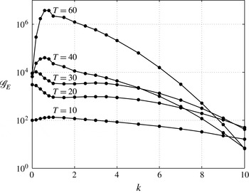
Influence of the horizon time $T$ on the optimal energy gain $\mathscr{G}_{E}$ as a function of the spanwise wavenumber $k$ of the optimal perturbation at $\mathit{At}=0$ .

A thorough validation of the numerical tool has been conducted in Lopez-Zazueta (Reference Lopez-Zazueta2015) but we restrict it here to a short presentation of the optimal perturbation in the homogeneous case for a Reynolds number of $\mathit{Re}=1000$ which corresponds to the work of Arratia et al. (Reference Arratia, Caulfield and Chomaz2013). The figure 3 shows the optimal energy gain $\mathscr{G}_{E}$ obtained for various horizon times of a perturbation injected in the flow at $t_{0}=0$ . The agreement with the results of Arratia et al. (Reference Arratia, Caulfield and Chomaz2013) is excellent, see their figure 5.

2.4 Diagnostics

In order to understand the physical mechanisms associated with the energy growth of the optimal perturbations, it is useful to specify some diagnostics such as the evolution equation for the growth rate of the perturbation $\unicode[STIX]{x1D70E}_{E}=(1/E)\,\text{d}E/\text{d}t$ . It is obtained straightforwardly from the transport equation for the perturbation kinetic energy $E=\Vert \boldsymbol{q}\Vert _{u}$ which reads

where $\unicode[STIX]{x1D6F1}_{E1}$ is the energy production/destruction by the base-flow shear, $\unicode[STIX]{x1D6F1}_{E2}$ the energy production/destruction by the base-flow strain field, $\unicode[STIX]{x1D6F1}_{E3}$ is the energy production/destruction coming form the coupling of density and pressure fields, $\unicode[STIX]{x1D6F1}_{E4}$ is the energy production/destruction by the base-flow dilatation/compression and $\unicode[STIX]{x1D6F1}_{E\unicode[STIX]{x1D719}}$ is the viscous dissipation. Both $\unicode[STIX]{x1D6F1}_{E3}$ and $\unicode[STIX]{x1D6F1}_{E4}$ terms are specific to the variable-density situation and are not present in the homogeneous case, see equation (4.1) of Arratia et al. (Reference Arratia, Caulfield and Chomaz2013). $\unicode[STIX]{x1D6F1}_{E3}$ corresponds to the remnant of the baroclinic vorticity production in the kinetic energy equation. For this reason, we will refer simply to it as the ‘baroclinic’ energy production hereinafter even if the semantic is not properly suited when dealing with the kinetic energy budget. Furthermore, because $\unicode[STIX]{x1D6F1}_{E4}$ is always very small, we chose to combine it with $\unicode[STIX]{x1D6F1}_{E2}$ in all the results presented in the paper.

Since the specificity of the variable-density flows considered here lies essentially in the baroclinic vorticity production, it is also useful to derive the linearised version of the vorticity equation (2.4) which writes

where $\boldsymbol{b}$ is the linearised baroclinic torque defined by

Pressure terms (i) and (ii) can be recast using an appropriate combination of the momentum equation for the base flow and for the perturbation. Given that $\mathit{Re}=1000$ , the viscous terms appearing in $\boldsymbol{b}$ are very small compared to the inertial terms and will be neglected in the following. Hence, the linearised baroclinic torque simplifies to

with $\boldsymbol{a}$ and $\boldsymbol{A}$ the linearised acceleration fields of the perturbation and the base flow respectively

From the vorticity transport equation (2.16), it is straightforward to derive an equation for the perturbation enstrophy $Z=\iint \unicode[STIX]{x1D74E}^{\ast }\unicode[STIX]{x1D74E}\,\text{d}x\,\text{d}y$ :

where $\unicode[STIX]{x1D6F1}_{Z1}$ is the enstrophy production/destruction by the base-flow shear, $\unicode[STIX]{x1D6F1}_{Z2}$ the enstrophy production/destruction by the base-flow strain field, $\unicode[STIX]{x1D6F1}_{Z3}$ is the enstrophy production/destruction by the base-flow spanwise vorticity advection by the perturbation, $\unicode[STIX]{x1D6F1}_{Z4}$ is the enstrophy production/destruction by vortex stretching, $\unicode[STIX]{x1D6F1}_{Z5}$ the enstrophy production/destruction by the base-flow dilatation/compression, $\unicode[STIX]{x1D6F1}_{Z6}$ the enstrophy production/destruction by dilatation/compression of the perturbation, $\unicode[STIX]{x1D6F1}_{Z7}$ the baroclinic enstrophy production/destruction and $\unicode[STIX]{x1D6F1}_{Z\unicode[STIX]{x1D719}}$ is the viscous dissipation. The three terms $\unicode[STIX]{x1D6F1}_{Z5}$ , $\unicode[STIX]{x1D6F1}_{Z6}$ and $\unicode[STIX]{x1D6F1}_{Z7}$ are specific to the variable-density case. In the following of the paper, all terms that do not contribute significantly to the enstrophy budget will be gathered conveniently according to the cases considered.

3.1 Optimal energy growth

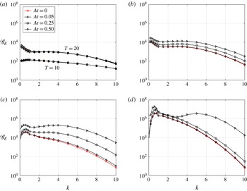
We first consider the optimal perturbations developing in the variable-density mixing layer when injected at the initial time of the development of the base flow, i.e. $t_{0}=0$ . Figure 4 displays the optimal energy gain $\mathscr{G}_{E}$ as a function of the spanwise wavenumber $k$ for different Atwood numbers and different horizon times ranging from $T=10$ to $T=60$ . For short optimisation times ( $T\lesssim 20$ ), the optimal energy growth is almost insensitive to the density variations since the curves in figure 4(a) are superimposed on each other. In that case, the interval of optimisation lies within the period of linear evolution of the primary KH wave during which the base flow remains quasi-parallel. 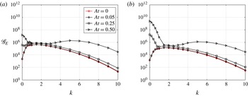When the horizon time is set equal to the saturation time of the primary KH mode ( $T=t_{KH}=30$ ), the optimal energy gain depends on the Atwood number as seen in figure 4(b). All amplification curves follow the same trend but the optimal energy gain is getting larger with increasing Atwood number. For optimisation times beyond $t_{KH}$ , the influence of the Atwood number on the optimal energy growth is even more pronounced and the increase is not homogeneously spread amongst the spanwise wavenumbers. Optimal perturbations with large spanwise wavenumber benefit more from the variable-density effects than those with small spanwise wavenumber. This is readily observable in figure 4(c) for $T=40$ but the difference is clear in figure 4(d) for $T=60$ . Despite this unequal gain enhancement, the overall maximum energy gain, associated with the so-called global optimal perturbation, always corresponds to a small spanwise wavenumber ( $k<1$ ), at least for the present moderate Reynolds number.

Figure 4.

Influence of the Atwood number on the energy gain $\mathscr{G}_{E}$ as a function of the spanwise wavenumber $k$ of the optimal perturbation for various horizon time: (a) $T=[10,20]$ , (b) $T=30$ , (c) $T=40$ and (d) $T=60$ .

Figure 5.

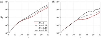
Temporal evolution of the optimal energy gain $\mathscr{G}_{E}$ for various Atwood numbers: optimal perturbation for $T=40$ with (a) $k=0.6$ and (b) $k=4$ . The bullet points denote the optimisation time.

This difference in the increase of amplification is also observable in figure 5 where the temporal evolution of the energy gain is displayed until $t=60$ for two perturbations optimised for $T=40$ . The first one is the global optimal which corresponds to a small spanwise wavenumber, $k=0.6$ and the second one is a perturbation with a large wavenumber, $k=4$ . In the homogeneous case, they correspond respectively to perturbations leading to the development of an elliptic and a hyperbolic instability (Arratia et al. Reference Arratia, Caulfield and Chomaz2013). Just like these authors, we adopt the same terminology in the following of the paper: elliptical E-type and hyperbolic H-type perturbations will refer to optimal perturbations which develop respectively in the core and in the braid of the main structure. In agreement with the above observation, the initial evolution of their energy growth does not depend on the Atwood number. The influence of density variations is felt a little before $t=20$ for the E-type perturbation while it starts a little after $t=20$ for the H-type one. Hence, there are substantial changes in the base flow around that time which induce a significant modification of the optimal perturbation with increasing Atwood number. By $t=20$ , the baroclinic vorticity production has become substantial so that the vorticity field of the VDKH billow departs significantly from its homogeneous counterpart: the asymmetry of the vortex core as well as the intense layering of the stretched vorticity braid are distinctly observable, especially as the Atwood number is increased. For this reason we can introduce a bifurcation time, denoted $t_{b}\approx 20$ , which clearly separates the evolution of the optimal perturbation into two periods provided that $T>t_{b}$ : an initial one $[0,t_{b}]$ with a unique route for energy growth whatever the Atwood number, and a second one $[t_{b},T]$ where density variations have a strong influence on the evolution of the optimal perturbation. In the following, we analyse each stage separately in order to identify the physical mechanisms at play in the growth of the optimal perturbation and elucidate the reason for this patent separation.

Figure 6.

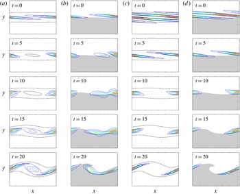
Temporal evolution of the energy field of the optimal perturbation during the time interval $[0,t_{b}]$ . The perturbation is optimised for $T=40$ with from (a) to (d): $\mathit{At}=0,k=0.6$ (a), $\mathit{At}=0.5,k=0.6$ (b), $\mathit{At}=0,k=4$ (c) and $\mathit{At}=0.5,k=4$ (d). In the homogeneous case, the dashed contour corresponds to $20\,\%$ of the maximal absolute value of the base-flow vorticity $|\unicode[STIX]{x1D6FA}_{m}|$ .

Figure 7.

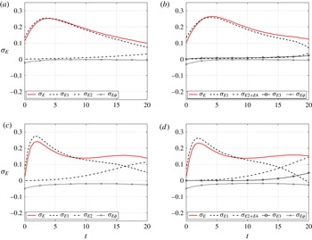
Temporal evolution of the kinetic energy growth rate $\unicode[STIX]{x1D70E}_{E}$ and its different contributions for the optimal perturbation during the time interval $[t_{0},t_{b}]$ according to equation (2.15). The perturbation is optimised for $T=40$ with (a) $k=0.6,\mathit{At}=0$ , (b) $k=0.6,\mathit{At}=0.5$ , (c) $k=4,\mathit{At}=0$ and (d) $k=4,\mathit{At}=0.5$ .

Figure 8.

Initial ratio between the contribution to enstrophy of the longitudinal and the spanwise components of the vorticity $f=\iint \unicode[STIX]{x1D714}_{x}^{2}(t_{0})\,\text{d}x\,\text{d}y/\iint \unicode[STIX]{x1D714}_{z}^{2}(t_{0})\,\text{d}x\,\text{d}y$ as a function of the spanwise wavenumber $k$ of the optimal perturbation optimised at $T=40$ for $\mathit{At}=0$ and $\mathit{At}=0.5$ .

3.2 First period $[0,t_{b}]$

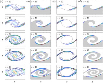
Figure 6 presents the early evolution of the field of the perturbation kinetic energy for the two same optimal perturbations considered in figure 5. The first and third columns correspond respectively to the evolution of perturbations in the homogeneous case at small and large wavenumbers: the E-type perturbation with $k=0.6$ , which is also the global optimal, and the H-type perturbation with $k=4$ . The second and fourth columns display their equivalent in the most density-contrasted case $\mathit{At}=0.5$ . For both types of perturbations and for homogeneous as well as for the inhomogeneous cases, the energy is initially concentrated in a thin layer centred around the hyperbolic braid saddle point and orientated along the direction of maximum compression of the base flow. When comparing both the homogeneous and the inhomogeneous cases, one can denote in the later a slight asymmetry of the energy field. The peak of energy is displaced towards the left side of the braid that will eventually roll-up into the billow on the light side of the mixing layer. This asymmetry anticipates the asymmetric development of the VDKH billow on the same pattern described in § 2.2. As the base flow evolves under the growth of the primary KH wave, the layers are progressively deformed under the action of the base-flow mean shear in such way so as to be realigned in the direction of the maximal stretching of the mixing layer. For the hyperbolic perturbation the energy stays concentrated in the braid region while for the elliptic one it progressively spreads out in the central zone where the core of the growing KH billow will be located.

The associated energy growth during this period is essentially due to base-flow shear conversion as can be seen in figure 7 which presents the temporal evolution of the energy growth rate budget according to equation (2.15) for the same four previous perturbations. By the end of the period around $t\sim 15$ , the energy growth is also supplied by the base-flow strain conversion for the H-type perturbations. As expected from previous observations, the density variations have almost no influence on the kinetic energy budget during this period. 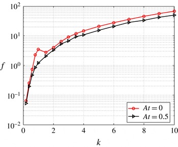For $\mathit{At}=0.5$ , the baroclinic term $\unicode[STIX]{x1D70E}_{E3}$ remains close to zero and the other contributions to the growth rate do not differ from the homogeneous case. This initial energy growth is due to the synergy of both classical Orr and lift-up transient mechanisms, as already observed by Arratia et al. (Reference Arratia, Caulfield and Chomaz2013) in the homogeneous case. The Orr mechanism is associated with the kinematic deformation of initial spanwise vorticity patches under the action of the base-flow mean shear while the lift-up mechanism corresponds the emergence of longitudinal streaks of high and low velocity under the action of the base-flow mean shear onto an initial perturbation made of an array of longitudinal vortices. Hence, the relative contribution of each mechanism to the growth of the perturbation can be assessed through the ratio $f=\iint \unicode[STIX]{x1D714}_{x}^{2}(t_{0})\,\text{d}x\,\text{d}y/\!\iint \unicode[STIX]{x1D714}_{z}^{2}(t_{0})\,\text{d}x\,\text{d}y$ between the contribution of the longitudinal and the spanwise components of the vorticity to the perturbation enstrophy at the injection time. This quantity is displayed in figure 8 as a function of the spanwise wavenumber $k$ and shows that E-type optimal perturbations ( $f\lesssim 1$ ) are initially structured to take advantage of the Orr mechanism at low wavenumber while H-type ones ( $f>1$ ) are initially organised to benefit from the lift-up mechanism at higher wavenumbers.

Figure 9.

Temporal evolution of the energy field of the optimal perturbation during the time interval $[t_{b},T]$ . The perturbation is optimised for $T=40$ with $\mathit{At}=0,k=0.6$ (a), $\mathit{At}=0.5,k=0.6$ (b), $\mathit{At}=0,k=4$ (c) and $\mathit{At}=0.5,k=4$ (d).

Figure 10.

Temporal evolution of the kinetic energy growth rate $\unicode[STIX]{x1D70E}_{E}$ and its different contributions for the optimal perturbation during the time interval $[t_{0},60]$ according to equation (2.15). The perturbation is optimised for $T=40$ with (a) $k=0.6,\mathit{At}=0$ , (b) $k=0.6,\mathit{At}=0.5$ , (c) $k=4,\mathit{At}=0$ and (d) $k=4,\mathit{At}=0.5$ .

3.3 Second period $[t_{b},T]$

We now focus on the second period of the development of the optimal perturbations after the bifurcation time. At this stage, the influence of the Atwood number is substantial as can be seen from figure 9 where the structure of the perturbations at $\mathit{At}=0.5$ departs clearly from the homogeneous case. As for the perturbation with a small wavenumber, the energy concentrates essentially into two asymmetric thin layers located along the braid of the VDKH billow. This asymmetry between the layers is imposed by the asymmetric development of the primary roll-up discussed in § 2.2. Even if some small amount of energy still lies within the core of the primary structure, most of it is concentrated within the two thin layers located along the braid. This pattern is not comparable to the one observed in the homogeneous case. We conclude that the perturbation cannot be labelled as an E-type perturbation anymore but that it is rather an H-type one as it concentrates in the braid region. This change in the nature of the perturbation is not that surprising if one refers to the results of the modal analysis of Fontane & Joly (Reference Fontane and Joly2008) performed at the saturation time of the primary wave. It was found that the growth rate $\unicode[STIX]{x1D70E}_{r}$ of the elliptic modes were insensitive to the increase of the Atwood number while the hyperbolic ones were strongly enhanced by density effects. In the $(k,\unicode[STIX]{x1D70E}_{r})$ plane, this resulted in the progressive drift of the elliptic modes towards the group of weakly amplified modes so that they could not even be identified with the modal analysis at $\mathit{At}=0.5$ (see figure 4 of Fontane & Joly Reference Fontane and Joly2008). Hence, the computation of several sub-optimal perturbations (not performed here) would be required in order to exhibit an E-type perturbation at $k=0.6$ . On the other hand, the large wavenumber perturbation is developing on a similar pattern than the small wavenumber one but with no energy located within the core of the VDKH billow. It remains clearly an H-type perturbation.

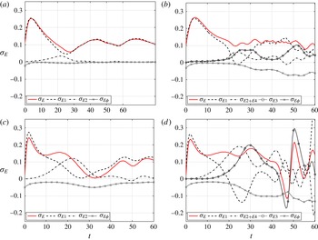
Figure 10 displays the temporal evolution of the kinetic energy growth rate $\unicode[STIX]{x1D70E}_{E}$ and its different contributions according to equation (2.15). In the homogeneous case, nearly all the energy of the E-type perturbation at $k=0.6$ comes from the base-flow shear conversion $\unicode[STIX]{x1D70E}_{E1}$ as already observed by Arratia et al. (Reference Arratia, Caulfield and Chomaz2013) (see their figure 7). In the density-contrasted situation, this term still provides the largest contribution to the energy growth throughout the optimisation period but both the baroclinic term $\unicode[STIX]{x1D70E}_{E3}$ and the base-flow strain conversion $\unicode[STIX]{x1D70E}_{E2}$ contribute significantly to the growth of the perturbation after the bifurcation time. For large wavenumbers, the H-type perturbation at $k=4$ in the homogeneous case extracts energy from the base flow alternatively through the shear $\unicode[STIX]{x1D70E}_{E1}$ and strain $\unicode[STIX]{x1D70E}_{E2}$ terms, in agreement with Arratia et al. (Reference Arratia, Caulfield and Chomaz2013). In the inhomogeneous case, the picture is more complex with a combined contribution of all terms of the equation (2.15), none of them being predominant and each one turning intermittently into a sink term during the time interval. One can also notice that both small and large wavenumber perturbations share a common feature in the variable-density case. After the bifurcation time $t_{b}$ , there is a substantial increase of the dissipation term $\unicode[STIX]{x1D70E}_{E\unicode[STIX]{x1D719}}$ compared to their homogeneous counterparts. This is related to the structuring of the optimal perturbation on thin layers associated with larger gradients yielding enhanced viscous dissipation.

This detailed analysis of the perturbation kinetic energy budget only enables us to identify major contributions to the perturbation growth but fails at giving an understanding of the physical mechanisms associated with the observed extra energy growth. As mentioned previously in § 2, the specificity of these variable-density flows compared to their homogeneous counterparts is best understood from their vorticity dynamics. Thus, we now examine carefully the perturbation enstrophy budget and we focus first on the global optimal perturbation corresponding to small spanwise wavenumber before considering optimal perturbations with larger $k$ .

Figure 11.

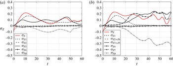
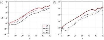
Temporal evolution of the enstrophy $Z$ and the relative contribution of each vorticity component $\unicode[STIX]{x1D714}_{x},\unicode[STIX]{x1D714}_{y}$ and $\unicode[STIX]{x1D714}_{z}$ for the global optimal perturbation during the time interval $[t_{0},60]$ . The perturbation is optimised for $T=40$ with (a) $\mathit{At}=0$ and (b) $\mathit{At}=0.5$ .

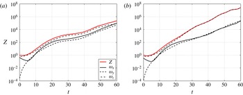
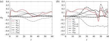
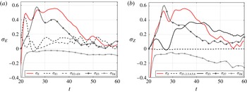
Figure 11 shows the temporal evolution of the enstrophy $Z$ of the global optimal at $\mathit{At}=0$ and $\mathit{At}=0.5$ together with the relative contribution of each vorticity component. Not only the enstrophy growth in the variable-density case is enhanced after the bifurcation time but it is also clearly due to the growth of spanwise vorticity component $\unicode[STIX]{x1D714}_{z}$ when all vorticity components contribute equally in the homogeneous case. Considering the temporal evolution of the enstrophy growth rate $\unicode[STIX]{x1D70E}_{Z}$ and its different contributions according to equation (2.20) plotted in figure 12, one can see that the main difference lies in the substantial increase of the baroclinic vorticity production $\unicode[STIX]{x1D70E}_{Z7}$ . It onsets around the bifurcation time and remains the main source of enstrophy together with the advection term $\unicode[STIX]{x1D70E}_{Z3}$ , already active in the homogeneous case. The base-flow shear conversion term $\unicode[STIX]{x1D70E}_{Z1}$ , which provides the main contribution to the enstrophy growth during the first period $[t_{0},t_{b}]$ , quickly goes to zero after the bifurcation time while it remains a significant source of enstrophy in the homogeneous case. As observed for the kinetic energy, the variable-density effects are also responsible for a significant increase of the enstrophy dissipation owing to the development of small scales and to the layered structure of the perturbation vorticity field (see figure 14 b). The extra dissipation is overcompensated by a larger increase of the $\unicode[STIX]{x1D70E}_{Z3}$ term after $t_{b}$ yielding larger growth.

Figure 12.

Temporal evolution of the enstrophy growth rate $\unicode[STIX]{x1D70E}_{Z}$ and its different contributions for the global optimal perturbation during the time interval $[t_{0},60]$ according to equation (2.20). The perturbation is optimised for $T=40$ with (a) $\mathit{At}=0$ and (b) $\mathit{At}=0.5$ .

Figure 13.

Temporal evolution of the ratio between the two terms constituting the spanwise component of the linearised baroclinic torque (3.1). The perturbation is optimised for $T=40$ with $k=0.6$ and $\mathit{At}=0.5$ .

Figure 14.

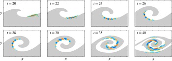
Temporal evolution of density $\unicode[STIX]{x1D70C}$ (a), spanwise vorticity $\unicode[STIX]{x1D714}_{z}$ (b) and longitudinal velocity $u_{x}$ (c) of the global optimal perturbation during the time interval $[t_{b},T]$ . The perturbation is optimised for $T=40$ with $\mathit{At}=0.5$ .

We now analyse in detail the contribution of the baroclinic torque to the growth of the optimal perturbation. The spanwise component $b_{z}$ of the linearised baroclinic torque (2.17) comes as the sum of two contributions:

Figure 15.

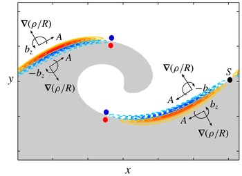
Spanwise component of the linear baroclinic torque $b_{z}$ at $t=25$ for the global optimal perturbation together with a schematic representation of the contribution of term $b_{z_{2}}$ sketched on top of it. Red and blue dots indicate the local sign of the spanwise vorticity of the perturbation before the action of the baroclinic torque at time $t_{b}$ .

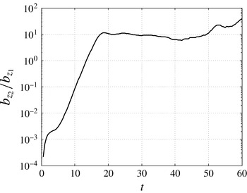
The first term $b_{z_{1}}$ corresponds to the cross-product between the acceleration of the perturbation and the base-flow density field while the second one $b_{z_{2}}$ is the cross-product between the acceleration of the base flow and the perturbation density field. The temporal evolution of the ratio between both terms $b_{z_{2}}/b_{z_{1}}$ is plotted in figure 13. 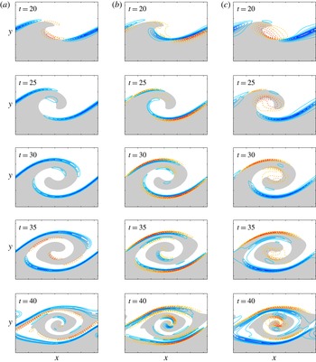The term $b_{z_{2}}$ becomes predominant a little before $t_{b}$ by an order of magnitude and is responsible for the substantial increase of the spanwise perturbation vorticity. Looking at the evolution of the perturbation density field during the interval $[t_{b},T]$ in figure 14(a), it is mainly structured in a thin layer of negative density located along the braid. Combined with the two-dimensional base-flow acceleration field in the hyperbolic braid region, it results in a contribution of term $b_{z_{2}}$ organised into a quadrupole centred on the braid saddle point $S$ as sketched in figure 15 for $t=25$ . This distribution is consistent with the contribution of the linear baroclinic torque $b_{z}$ also plotted in figure 15. At the bifurcation time, the spanwise perturbation vorticity $\unicode[STIX]{x1D714}_{z}$ consists of two elongated layers of opposite sign along the braid as can be seen in figure 14(b). In the half of the braid located on the left side of the saddle point, the baroclinic torque contributions are of the same sign as the current perturbation spanwise vorticity indicated by the coloured bullet points in figure 15. Thus, they locally enhance the two existing layers of perturbation vorticity. Conversely, in the half of the braid located on the right side of the saddle point, the two spanwise baroclinic production terms are of opposite sign to the one of the local vorticity field and contribute to its destruction. As displayed in figure 14(b), the spanwise vorticity layers in the right-upper part of the braid are quickly cancelled under the action of the baroclinic torque before being replaced by two layers of opposite sign which are readily observable at $t=25$ . By $t=30$ , the spanwise vorticity field of the perturbation is structured on each side of the saddle point into two elongated layers of opposite sign according to spanwise vorticity baroclinic production. This pattern of elongated opposite shear layers is characteristic of longitudinal jets which is confirmed by looking at the perturbation longitudinal velocity field $u_{x}$ in the third column of figure 14(c). 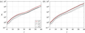At $t=30$ , it consists of two streaks of opposite sign located along the braid on either side of the saddle point. These streaks are responsible for the essential of the perturbation energy growth as shown in figure 16. While the contribution of each component of the velocity to the energy gain is isotropic in the homogeneous case, the energy growth is primarily due to the increase of the perturbation longitudinal velocity component in the variable-density case. This is corroborated by a similar evolution of the structure for both the longitudinal velocity field and the energy field in figures 14(c) and 9.

Figure 16.

Temporal evolution of the energy $E$ and the relative contribution of each velocity component $u_{x},u_{y}$ and $u_{z}$ for the global optimal perturbation during the time interval $[t_{0},60]$ . The perturbation is optimised for $T=40$ with (a) $\mathit{At}=0$ and (b) $\mathit{At}=0.5$ .

Figure 17.

Temporal evolution of (a) the enstrophy $Z$ and the relative contribution of each vorticity component $\unicode[STIX]{x1D714}_{x},\unicode[STIX]{x1D714}_{y}$ and $\unicode[STIX]{x1D714}_{z}$ and (b) the energy $E$ and the relative contribution of each velocity component $u_{x},u_{y}$ and $u_{z}$ for the optimal perturbation with $k=4$ during the time interval $[t_{0},60]$ . The perturbation is optimised for $T=40$ with $\mathit{At}=0.5$ .

Figure 18.

Temporal evolution of the enstrophy growth rate $\unicode[STIX]{x1D70E}_{Z}$ and its different contributions for the optimal perturbation with $k=4$ during the time interval $[t_{0},60]$ according to equation (2.20). The perturbation is optimised for $T=40$ with (a)  $\mathit{At}=0$ and (b) $\mathit{At}=0.5$ .

Figure 19.

(a) Density $\unicode[STIX]{x1D70C}$ , (b) spanwise baroclinic torque $b_{z}$ , (c) spanwise vorticity $\unicode[STIX]{x1D714}_{z}$ and (d) longitudinal velocity $u_{x}$ fields of the optimal perturbation at $t=30$ . The perturbation is optimised for $T=40$ with $k=4$ and $\mathit{At}=0.5$ .

Figure 20.

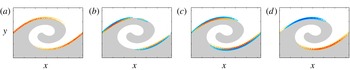
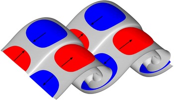
Illustration of the three-dimensionalisation process of variable-density free shear layers in the case of the global optimal perturbation at $t=30$ with $k=0.6$ , $T=40$ and $\mathit{At}=0.5$ . The grey surface corresponds to mean isopycnal of the perturbed VDKH billow. The red and blue regions denote the positive and negative longitudinal velocity streaks associated with the optimal perturbation at the same time, also indicated by the arrows. They correspond respectively to values of $0.2u_{x,max}$ and $0.2u_{x,min}$ .

The physical mechanism for energy growth described previously is generic for all optimal perturbations identified here whatever the value of the spanwise wavenumber. For larger wavenumber, the enstrophy and energy growth are also driven by the increase of the spanwise vorticity and longitudinal velocity respectively as illustrated in figure 17 for $k=4$ . The enstrophy budget in figure 18 attests that extra enstrophy growth is again related to the onset of the baroclinic vorticity production $\unicode[STIX]{x1D70E}_{Z7}$ . The main difference with the small wavenumber optimal perturbation is the contribution to the enstrophy growth of the base-flow strain conversion term $\unicode[STIX]{x1D70E}_{Z2}$ , which is already active in the homogeneous case. The same structure for the perturbation density field consisting of a thin layer located along the braid (figure 19 a) results in a similar quadrupolar pattern for the spanwise baroclinic torque (figure 19 b). It yields to the production of two thin layers of spanwise vorticity along the braid on either side of the saddle point (figure 19 c) which eventually give rise to the longitudinal velocity streaks (figure 19 d) responsible for the optimal energy growth (figure 17 b). Comparing figures 14 and 19, the sign difference between the perturbation fields only comes from the arbitrary phase associated with the $z$ -planes at which the fields are represented.

Figure 21.

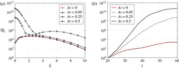
(a) Influence of the Atwood number on the energy gain $\mathscr{G}_{E}$ as a function of the spanwise wavenumber $k$ of the optimal perturbations in the interval $[t_{0},T]=[20,60]$ . (b) Temporal evolution in the interval $[t_{0},T]=[20,60]$ of the energy gain $\mathscr{G}_{E}$ for the optimal perturbation with $k=0$ and various Atwood numbers.

The optimal mechanism for energy growth elucidated here relies on the emergence on either side of the saddle point of longitudinal velocity streaks of opposite sign along the baroclinically enhanced vorticity braid of the primary VDKH billow. Figure 20 gives a three-dimensional view of this transitional scenario which differs completely from the promotion of rib vortices along the braid observed in the homogeneous case (Arratia et al. Reference Arratia, Caulfield and Chomaz2013) and so far accepted as the paradigm for three-dimensionalisation of free shear flows. If the route to three-dimensionalisation identified here is generic to all variable-density free shear flows, it calls into question the physical mechanism originally advocated by Monkewitz & Pfizenmaier (Reference Monkewitz and Pfizenmaier1991) and extended by Brancher et al. (Reference Brancher, Chomaz and Huerre1994) for the generation of the side jets occurring in light round jets. These authors claimed that the emergence of side jets relies on the velocity induction by the pairs of counter-rotating streamwise vortices associated with the secondary three-dimensional instabilities. The present analysis rather suggests that a more likely mechanism for side ejections would be based on the convergence of the two longitudinal velocity streaks of opposite sign near the braid saddle point. Although quite plausible, this conjecture must be examined further before being asserted. It would be interesting to look first at the three-dimensional nonlinear development of the optimal perturbation and scrutinise the velocity field in the crosswise plane located at the saddle point. Second, a similar non-modal analysis performed for round jets would confirm if this original route to three-dimensional motions is robust to the axisymmetrisation of the plane KH-rollers into a vortex ring. These perspectives are beyond the scope of the present study and are left to future work.

3.4 Influence of the injection time

Until this point the perturbations were optimised for a given horizon time $T$ by being injected in the flow at the initial time of the base-flow evolution, i.e. $t_{0}=0$ . The influence of the Atwood number on the energy growth of optimal perturbations has been found to be negligible during the initial period $[0,t_{b}]$ where the energy growth is due to a combination of the Orr and lift-up mechanisms. We probe the influence of the injection time $t_{0}$ setting the injection time as $t_{0}=t_{b}=20$ in order to skip the initial period of growth and see how it affects the evolution of the optimal perturbations.

The figure 21 presents the energy gain $\mathscr{G}_{E}$ as a function of the spanwise wavenumber $k$ and various Atwood numbers for the perturbations optimised during the interval $[t_{0},T]=[20,60]$ . In the homogeneous case, as already observed by Arratia et al. (Reference Arratia, Caulfield and Chomaz2013), the energy gain is reduced for all the spanwise wavenumbers except for the very large ones ( $k\gtrsim 8$ ) where a slight increase of the gain can be noticed when comparing figures 4(d) and 21(a). The reduction in energy gain, which is even more pronounced for perturbations with small wavenumber, is due to the shortening of the initial period during which the Orr and lift-up mechanisms are the most effective. Nevertheless, all the optimal perturbations still undergo a short initial phase of transient growth before evolving towards the elliptic and hyperbolic modes (Arratia et al. Reference Arratia, Caulfield and Chomaz2013). In the variable-density case, the picture is very different and displays a discontinuity in the curves for a given wavenumber $k_{c}$ which denotes the coexistence of two distinct branches corresponding to optimal perturbations of different nature. The spanwise wavenumber $k_{c}$ at which the two branches cross increases with the Atwood number. We measure $k_{c}\approx 1.7$ and $k_{c}\approx 2.8$ respectively for $\mathit{At}=0.25$ and $\mathit{At}=0.5$ . The perturbations of the first branch, corresponding to small spanwise wavenumbers, exhibit energy gain significantly larger than those of the second branch spanning the large wavenumbers. The largest gain of the first branch, which is also the overall maximum, corresponds to a two-dimensional perturbation, i.e. $k=0$ . It is also significantly higher than those observed in § 3.1. This strongly suggests that the optimal perturbation is of a very different nature from the one obtained for similar wavenumbers when the optimisation started from $t_{0}=0$ . Conversely, the second branch presents a maximum located around $k\approx 5.5$ and a shape which is very close to what was obtained for an optimisation from $t_{0}=0$ , indicating that the nature of the perturbation is likely to be the same for this range of wavenumbers.

To determine the nature and identify the physical mechanisms of energy growth behind the perturbation of the first branch, we analyse in detail the characteristics of the two-dimensional global optimal. The effect of the Atwood number on the evolution of the energy gain $\mathscr{G}_{E}$ is displayed in figure 21(b). It is remarkable to note that the perturbation reaches quickly energy levels much higher than those measured in homogeneous situation. By $t=25$ , the gain measured for $\mathit{At}=0.5$ is already twice the one obtained for $\mathit{At}=0$ . At the time horizon $T$ , the energy gain is respectively five and seven orders of magnitude higher for $\mathit{At}=0.25$ and $\mathit{At}=0.5$ respectively. The structure of the optimal perturbation consists of small elongated spanwise vorticity patches of alternate sign located along the braid on the left side of the saddle point as displayed in figure 22 at $t=20$ . As the primary KH wave overturns, the patches deform and move progressively towards the core of the VDKH billow following the central isopycnal $\unicode[STIX]{x1D70C}=\unicode[STIX]{x1D70C}_{0}$ . This perturbation corresponds to the secondary KH instability of the baroclinically enhanced vorticity braid identified in the modal stability analysis of Fontane & Joly (Reference Fontane and Joly2008) and originally discovered by Reinaud et al. (Reference Reinaud, Joly and Chassaing2000).

Figure 22.

Temporal evolution of the spanwise vorticity field $\unicode[STIX]{x1D714}_{z}$ for the global optimal perturbation during the time interval $[t_{0},40]$ . The perturbation is optimised for $t_{0}=20$ and $T=60$ with $k=0$ and $\mathit{At}=0.5$ .

Figure 23.

Temporal evolution of (a) the kinetic energy growth rate $\unicode[STIX]{x1D70E}_{E}$ according to equation (2.15) and (b) the enstrophy growth rate $\unicode[STIX]{x1D70E}_{Z}$ according to equation (2.20) for the perturbation optimised during the interval $t=[20,60]$ with $k=0$ and $\mathit{At}=0.5$ .

The evolution of the perturbation can be decomposed into three stages when considering the temporal evolution of both the energy and enstrophy growth rate budgets in figure 23. The early initial energy growth, $20\leqslant t\lesssim 22$ , of the two-dimensional optimal perturbation is due to the Orr mechanism. As shown in figure 22, at the injection time $t_{0}=20$ , the vorticity patches are orientated in the direction corresponding locally to the maximal compression of the stretched braid. Then, while being convected towards the core of the VDKH billow, the patches are immediately tilted into the direction of the local maximal stretching under the action of the base-flow shear. During this kinematic deformation, the perturbation extracts energy from base-flow shear conversion relying on the Orr mechanism. This is confirmed in figure 23(a) where one can see a strong increase of the $\unicode[STIX]{x1D70E}_{E1}$ term which is the main contribution to the energy growth during this initial period. This transient contribution reaches its maximum around $t\sim 22$ before decreasing quickly.

The second stage of evolution, $22\lesssim t\lesssim 30$ , is characterised by an intense baroclinic production of vorticity as denoted by the sudden increase of term $\unicode[STIX]{x1D70E}_{Z7}$ in figure 23(b) which becomes the main contributor to the perturbation enstrophy growth. It is worth noting that the enstrophy budget simply relies on the balance between three terms throughout the perturbation evolution: the term $\unicode[STIX]{x1D70E}_{Z3}$ of production by base-flow spanwise vorticity advection by the perturbation, the baroclinic production $\unicode[STIX]{x1D70E}_{Z7}$ and the viscous dissipation $\unicode[STIX]{x1D70E}_{Z\unicode[STIX]{x1D719}}$ . During this stage, the vorticity production is very intense because the structure of the spanwise baroclinic torque presents a distribution of alternated sources and sinks that closely matches the perturbation spanwise vorticity field as can be seen in figure 24. This baroclinic production of vorticity is directly connected to the energy growth of the perturbation via the term of energy production $\unicode[STIX]{x1D70E}_{E3}$ which prevails over other source terms and allows the perturbation to keep on growing once the Orr mechanism is stopped, see figure 23(a). By $t=30$ , the pattern of the vorticity patches is similar to that associated with the classic KH shear instability.

Figure 24.

Temporal evolution of the spanwise component of baroclinic torque $b_{z}$ for the global optimal perturbation during the time interval $[24,30]$ . The perturbation is optimised for $t_{0}=20$ and $T=60$ with $k=0$ and $\mathit{At}=0.5$ .

After $t\gtrsim 30$ , the baroclinic contribution $\unicode[STIX]{x1D70E}_{E3}$ to the energy growth decreases down to levels equivalent to the other sources terms of shear conversion $\unicode[STIX]{x1D70E}_{E1}$ and of strain conversion $\unicode[STIX]{x1D70E}_{E2}$ . The energy growth rate of the perturbation decreases consequently and from $t\sim 40$ , the energy growth of the perturbation is slowed down significantly (see figure 21(b)) due to the combined decrease of $\unicode[STIX]{x1D70E}_{E3}$ term and a slight increase of the viscous dissipation $\unicode[STIX]{x1D70E}_{E\unicode[STIX]{x1D719}}$ . By the end of the optimisation interval, the energy growth rate is close to zero and the energy gain $\mathscr{G}_{E}$ plateaus, see figure 21(b).

The emergence of this secondary two-dimensional KH instability relies on the base-flow baroclinic vorticity production in the braid. As demonstrated by Dritschel et al. (Reference Dritschel, Haynes, Juckes and Shepperd1991), the instability can onset only if the local amount of vorticity is high enough to overcome the stabilising effect of the local stretching field in the braid. For this reason, the instability is not observed in homogeneous mixing layers where the magnitude of the vorticity field in the braids is too weak. As shown by Reinaud et al. (Reference Reinaud, Joly and Chassaing2000) and Fontane & Joly (Reference Fontane and Joly2008), the nonlinear development of this type of instability leads to the formation of smaller secondary vortical structures similar to the primary VDKH billow, opening the way to a cascade of two-dimensional KH rollers of smaller and smaller size (Fontane, Joly & Reinaud Reference Fontane, Joly and Reinaud2008). This unlikely two-dimensional transition to turbulence is radically different from both the one relying on homogeneous rib vortices or the one relying on the longitudinal velocity streaks, as found in the previous section for the variable-density case. Compared to the modal analysis of Fontane & Joly (Reference Fontane and Joly2008), the present work allows us to discuss a little further the competition between the two scenarios identified in the variable-density case. The secondary KH perturbation being only observed when the injection time is delayed, it is likely that the development of three-dimensional hyperbolic modes from the initial time of the flow evolution would preclude a purely two-dimensional scenario in natural variable-density mixing layers. Besides, the two-dimensional secondary KH mode has not been observed experimentally so far. Nevertheless, additional calculations displayed in figure 25, show that the two-dimensional optimal perturbation becomes the global optimal for $\mathit{At}=0.5$ when the injection time is as small as $t_{0}=10$ . Turning towards spatially developing mixing layers, the experimental evidence of such a striking two-dimensional response may require to delay the two-dimensional forcing at some distance downstream the splitter plate. Such an experiment is not straightforward and would certainly require a complex and very challenging experimental set-up.

The optimal perturbations of the second branch correspond to development of the same three-dimensional hyperbolic modes observed when the injection time is $t_{0}=0$ . They follow the same physical mechanism described in § 3.3 leading to the emergence of the longitudinal velocity streaks in the braid region. A further description of these perturbations would not bring any new information and is thus not necessary at this point.

Figure 25.

Influence of the Atwood number on the energy gain $\mathscr{G}_{E}$ as a function of the spanwise wavenumber $k$ of the optimal perturbations in the interval (a)  $[t_{0},T]=[10,60]$ and (b) $[t_{0},T]=[15,60]$ .