I

Derek Parfit described what he called the priority view and what is now usually called prioritarianism in the following way: “Benefitting people matters more the worse off these people are” (Parfit Reference Parfit, Clayton and Williams1991, 19). There is some disagreement about how to interpret Parfit’s proposal (see, e.g., Eyal and Herlitz Reference Eyal and Herlitz2023), but many proponents take it to mean that we ought to evaluate and rank distributive options “according to the sum of a strictly increasing and strictly concave transformation of individual well-being” (Adler and Holtug Reference Adler and Holtug2019, 101). In other words, options should be ranked by summing up priority-weighted well-being levels and the priority weights should be such that the lower the well-being, the greater the priority weight. In the literature on social welfare functions, the prioritarian welfare function is typically described in the following way:

$$\mathop \sum \limits_{i = 1}^n g\left( {{w^i}} \right)$$

where ${w^i}$ is the well-being of individual $i$ and $g( \cdot )$ is strictly increasing and strictly concave (or “backward-bending”).Footnote ¹

One obvious theoretical challenge with operationalizing prioritarianism is that it requires that all well-being levels can be represented with some cardinal scale.Footnote ² First, prioritarianism requires a “unit” of benefits that is common for all individuals. Moreover, unlike measurements such as temperature, the baseline or reference point can be significant. In other words, the absolute level of benefits itself plays an important role.Footnote ³ For the purposes of this paper, we assume that well-being levels are perfectly cardinal and set aside questions about this assumption’s plausibility.

The focus of this paper is another well-known question, namely the issue of what well-being to look at: should the prioritarian welfare function be applied to the well-being of individuals during sub-lifetime time periods or should it be applied to the well-being that individuals enjoy over their entire lives?Footnote ⁴ Outcome 1 brings out the issue:

Outcome 1

Long description

A table comparing outcomes for two individuals over two time periods and their lifetime. The table has three columns labeled t = 1, t = 2, and Lifetime, and two rows labeled Individual A and Individual B. Row 1: Individual A, t = 1, w subscript 1 superscript A; t = 2, w subscript 2 superscript A; Lifetime, w subscript L superscript A. Row 2: Individual B, t = 1, w subscript 1 superscript B; t = 2, w subscript 2 superscript B; Lifetime, w subscript L superscript B.

We note that $w_t^i$ denotes the well-being level of individual $i$ at the period $t$ , and $w_L^i$ is the well-being level of individual $i$ over their whole life.

According to one version of prioritarianism, Outcome 1 should be evaluated as follows:

$$g\left(w_L^A{}\right) + g\left(w_L^B\right)$$

This is the lifetime view. It looks at the sum of a strictly increasing and strictly concave transformation of individual lifetime well-being, i.e., the focus is on how well off individuals are over their entire lives. Insofar as lifetime well-being satisfies so-called separability of time such that the lifetime well-being of an individual is the sum of the well-being enjoyed during all sub-lifetime time periods and Individuals A and B only live during time periods 1 and 2, the lifetime-prioritarian evaluation of Outcome 1 could instead be the following (cf. Adler Reference Adler2012; Herlitz Reference Herlitz2018):

$$g\left( {w_1^A +w_2^A} \right) + g\left( {w_1^B + w_2^B} \right)$$

Moving forward, when discussing the lifetime view, we will assume that the well-being of interest is the sum of people’s temporal well-being so that $g \left( {w_1^A + w_2^A} \right)\, + g\left( {w_1^B + w_2^B} \right) = g\left(w_L^A\right) + g\left(w_L^B\right)$ .

A different version of prioritarianism evaluates Outcome 1 in this way (cf. McKerlie Reference McKerlie1997; Segall Reference Segall2016):Footnote ⁵

$$\left[ {g\left( {w_1^A} \right) + g\left( {w_1^B} \right)} \right] + \left[ {g\left( {w_2^A} \right) + g\left( {w_2^B} \right)} \right].$$

This is the timeslice view. It looks at the sum of a strictly increasing and strictly concave transformation of well-being being enjoyed by people during each time period, i.e., the focus is on how well off individuals are at different temporal periods.

A problem with lifetime prioritarianism is that it generates counterintuitive verdicts in certain kinds of cases. These are cases in which there are significant inequalities between people at different time periods, and these inequalities are distributed so that lifetime prioritarianism entails that it is better to benefit someone who is much better off at the time of receipt of benefit. Here is an illustration (where we use numbers to describe the amount of well-being enjoyed by a person at a time period):

Outcome 2

Long description

A table with two rows and seven columns comparing values for categories A and B over seven time points. The columns are labeled t = 1 through t = 7. Row A starts with a value of 1 at t = 1, increases to 10 from t = 2 to t = 6, and then decreases to 9 at t = 7. Row B maintains a constant value of 10 across all time points.

Outcome 3

Long description

A table with two rows and seven columns. The columns are labeled with time points t = 1 through t = 7. The rows are labeled A and B. Row A: t = 1, 1; t = 2, 10; t = 3, 10; t = 4, 10; t = 5, 10; t = 6, 10; t = 7, 10. Row B: t = 1, 10; t = 2, 10; t = 3, 10; t = 4, 10; t = 5, 10; t = 6, 10; t = 7, 5. The table shows the values for categories A and B across different time points.

Assume that having 10 units of well-being during a time period amounts to having a very good life at that time, that having 5 units of well-being during a time period amounts to having a mediocre life during that time, and that having 1 unit of well-being during a time period means that one leads a very poor life at that time.

The only difference between Outcomes 2 and 3 is what occurs at time period 7. In Outcome 2, A does not lead a very good life in time period 7, but they are still leading a good life. In Outcome 3, B leads a mediocre life in time period 7. In both outcomes, A leads a very poor life at time period 1. What lifetime prioritarianism says about this specific case depends on how much priority it ascribes to benefits to the worse off, but for some outcomes with well-being distributions with similar structure to the ones above, with a strongly concave prioritarian weighting function $g$ , lifetime prioritarianism will entail that Outcome 3 is better than Outcome 2, that it is better to give a small benefit to a person who is relatively well off than to give a much larger benefit to a significantly worse off person on the grounds that the (at the time) better off person led a bad life in the distant past. The reason is that the lifetime view violates separability of time in the sense that it ascribes priority weights to benefits at specific time periods based on what occurs also in other time periods, and although the time periods can be very far from each other, and the people with claims to benefits might not even remember them, the influence of these other time periods can mean that the view recommends giving smaller benefits to (at the time) better off people. This seems to run counter to the Parfitian idea that benefiting people matters more the worse off these people are.

More concretely, lifetime prioritarianism can entail that it is better to cure an old man’s hangnails than to offer hip-replacement to another old man (if, for instance, the first man had a significantly worse infancy). Or it can entail that an outcome in which all children are happy is worse than an outcome with one starving child and one child extra happy (if, for example, in the far future, the starving child leads a much better life than the extra happy child).

It is clear that timeslice prioritarianism avoids these implications. According to timeslice prioritarianism, time period 7 in Outcomes 2 and 3 is evaluated in isolation and that evaluation is unaffected by what occurs in other time periods. Since the outcomes are identical except for what occurs in time period 7, timeslice prioritarianism would evaluate the outcomes by comparing the following values:

$$g\left( 9 \right) + g\left( {10} \right){\rm{\;vs. \;} }g\left( {10} \right) + g\left( 5 \right)$$

Since $g( \cdot )$ is strictly increasing and strictly concave, it follows that $g\left( 9 \right)\, + g\left( {10} \right) \gt g\left( {10} \right) + g\left( 5 \right)$ . In other words, timeslice prioritarianism entails that Outcome 2 is better than Outcome 3. It is also obvious that timeslice prioritarianism will yield that verdict in all cases with this structure. It favors hip-replacement over curing hangnails and preventing starvation over making a happy child slightly happier.

However, also the timeslice view generates some very strange recommendations. One issue that has been underscored lately is that it recommends against seemingly perfectly benign “delay of gratification” (Andrić and Herlitz Reference Andrić and Herlitz2022; Cato and Hirose Reference Cato and Hirose2025). Consider the following pair of outcomes:

Outcome 4

Long description

A table with three columns and two rows. The columns are labeled t = 1, t = 2, and Lifetime. The row is labeled Individual A. For Individual A, the value under t = 1 is w, under t = 2 is w, and under Lifetime is 2w.

Outcome 5

Long description

A table with three columns and two rows. The columns are labeled t = 1, t = 2, and Lifetime. The row is labeled Individual A. The values in the table are as follows: Row 1: t = 1, w - α; t = 2, w + β; Lifetime, 2w - α + β.

Assume that $\alpha \gt 0\;$ and that $\beta \gt \alpha $ . Outcome 5 involves some delay of gratification. The individual foregoes some well-being at time period 1 but gains some larger amount of well-being at time period 2. This is the kind of thing that farmers do when they toil in order to bring in larger harvests at some later time, what students do when they study and accept simple lifestyles in order to be able to lead better lives after their studies, and so on. In many situations, it seems perfectly rational and unproblematic for individuals to do this.

Timeslice prioritarianism, however, sometimes entails that it is impermissible to delay gratification. What timeslice prioritarianism says about a specific case depends on how large the benefit of delaying gratification is and the specific nature of the priority weights. Let $\delta $ denote the benefit of delaying gratification, i.e., the difference between $\alpha $ and $\beta $ (i.e., $\delta = \beta - \alpha $ ). What timeslice prioritarianism says about a certain case depends on whether δ is large enough to counterbalance the impact of the priority weights.Footnote ⁶

Relatedly, timeslice prioritarianism does not satisfy the following, very appealing condition:

Here is an illustration of how the view violates Lifetime Pareto for Equal Distributions:

Outcome 6

Long description

A table with two rows and three columns. The columns are labeled t = 1 and t = 2. The rows are labeled Individual A and Individual B. Row 1: Individual A, t = 1, w; t = 2, w. Row 2: Individual B, t = 1, w; t = 2, w.

Outcome 7

Long description

A table with two rows and three columns. The columns are labeled t = 1 and t = 2. The rows are labeled Individual A and Individual B. For Individual A, at t = 1 the value is w - α and at t = 2 the value is w + β. For Individual B, at t = 1 the value is w - α and at t = 2 the value is w + β.

Lifetime Pareto for Equal Distributions entails that Outcome 7 is better than Outcome 6. However, assume, as before, that $\alpha \gt 0$ and that $\beta \gt \alpha $ . If $\delta = \left( {\beta - \alpha } \right)$ is not large enough to counterbalance the effects of the weighting function, timeslice prioritarianism entails that Outcome 6 is better than Outcome 7, although Outcome 7 contains no inequality at any time period, no inequality when the entire lives are compared, and although more total sum of well-being accrues to everyone.

There are two versions of prioritarianism discussed in the literature: lifetime prioritarianism and timeslice prioritarianism. Both face well-known challenges in that they generate problematic recommendations in some cases. Before introducing a new way for prioritarians to focus on time periods, we will in the next section introduce an essential element in that new view. To simplify the introduction of this element, we will set aside questions of what temporal periods matter.

II

In the literature on inequality measures, it is well-known that social welfare functions that rank different distributions will generate the same rankings if they instead are applied to equally distributed equivalents or EDE (see, e.g., Atkinson Reference Atkinson1970; Fleurbaey Reference Fleurbaey2010; Kolm Reference Kolm, Margolis and Guitton1969; Sen Reference Sen1973).Footnote ⁷ Given a social welfare function, the EDE of a distribution, D, is the amount of goods, $x$ , for which it is true that a distribution, E, in which each individual has $x$ is precisely as good as D with respect to the social welfare function.

Here is a very simple illustration. Let us assume a social welfare function that establishes the overall value of an outcome by summing up each individual’s amount of goods after the square root function has been applied to it. The square root function is strictly increasing and strictly concave so we can think of this as a very precise prioritarian social welfare function. Consider the following outcomes (where we use numbers to describe the amount of goods an individual has and set aside the issue of what temporal periods matter):

Outcome 8

Long description

A table with two rows and two columns. The columns are labeled Individual A and Individual B. Row 1: Individual A, 1; Individual B, 9.

Outcome 9

Long description

A table with two rows and two columns. The columns are labeled Individual and Outcome. The rows are labeled Individual A and Individual B. Row 1: Individual A, 4. Row 2: Individual B, 4.

Outcomes 8 and 9 are precisely as good with respect to the social welfare function under consideration. $\sqrt 1 + \sqrt 9 = 4$ , and $\sqrt 4 + \sqrt 4 = 4$ . Outcome 9 illustrates that 4 is the EDE of Outcome 8 with respect to the social welfare function.

More generally, consider a social welfare function f:

$$f\left( {{w^A},{w^B}} \right).$$

It is plausible to assume that f is anonymous in the sense that $f\left( {r,r'} \right) = f\left( {r',r} \right)$ for all real numbers $r,r'$ . Given the social welfare function, EDE is defined/obtained by:

$$f\left( {EDE,EDE} \right) = f\left( {{w^A},{w^B}} \right),$$

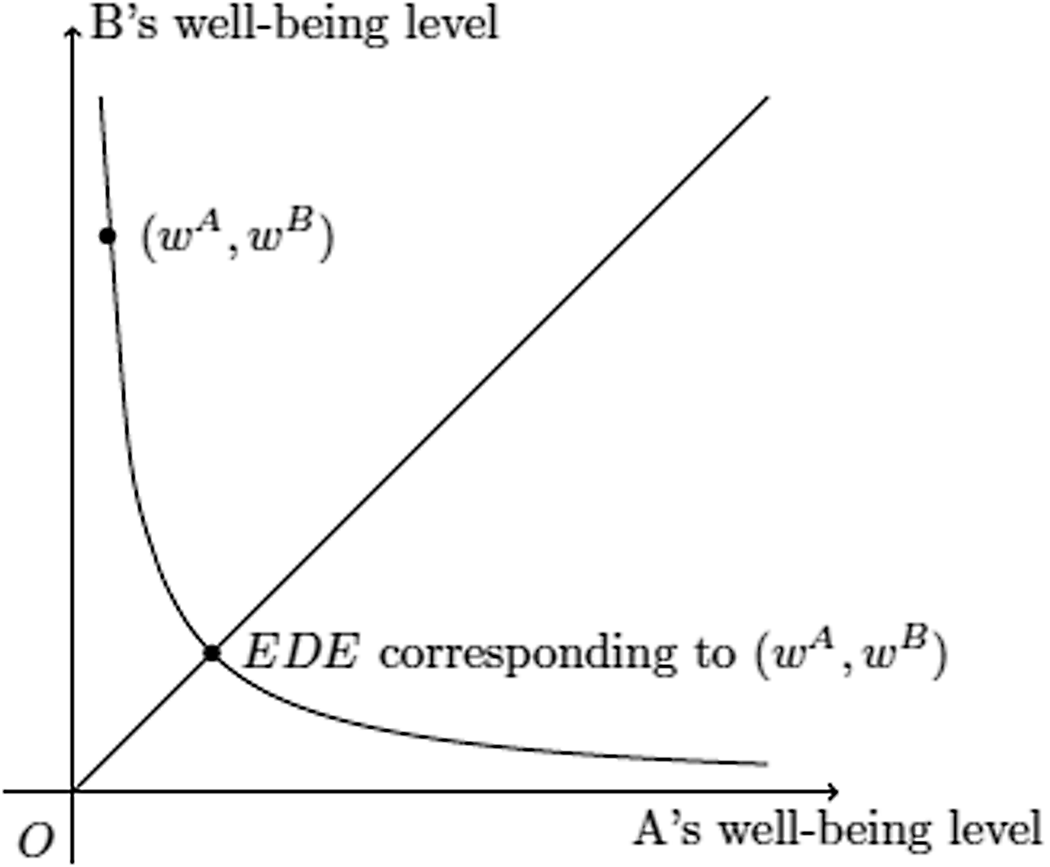
where ${w^A}$ is the well-being level of individual A and ${w^B}$ is that of individual B. As alluded to above, the EDE for distribution $\left( {{w^A},{w^B}} \right)$ is defined as the well-being level such that the original distribution is equally as good as a perfectly equal distribution where every person obtains this well-being level. The construction of the EDE is shown in Figure 1, where the curve crossing $\left( {{w^A},{w^B}} \right)$ is the “indifference curve” induced from f. In brief, the distance from the origin to the point where the social indifference curve intersects the 45-degree line represents the EDE. Importantly and by definition, EDE is ordinally equivalent to $f\left( {{w^A},{w^B}} \right)$ : $f\left( {{w^A},{w^B}} \right)$ is larger if and only if the corresponding EDE is larger. This means that rather than maximizing $f\left( {{w^A},{w^B}} \right)$ , a social planner can maximize EDE with the same result. As mentioned earlier, EDE is commonly utilized in the theory of inequality measures. Additionally, it plays a significant role in the literature on distributive justice (see, for instance, Bovens (Reference Bovens2015a, Reference Bovens2015b), Otsuka and Voorhoeve (Reference Otsuka, Voorhoeve and Olsaretti2018), and Voorhoeve (Reference Voorhoeve2021)).

Figure 1.

Construction of EDE.

Marc Fleurbaey has demonstrated that looking at EDE sometimes can offer new perspectives on social evaluations by looking at social evaluations of situations that involve risk (Fleurbaey Reference Fleurbaey2010). The context is the following: A famous theorem by John Harsanyi asserts that utilitarianism is the only rational theory that satisfies Ex ante Pareto, according to which a risky prospect is better if everyone’s expected well-being is higher (Harsanyi Reference Harsanyi1955, Reference Harsanyi1977).Footnote ⁸ However, assuming that the probabilities that the two states come about are the same (i.e., 0.5), Prospect 1 seems intuitively worse than Prospect 2 below:

Prospect 1

Long description

A table comparing states for two individuals. The table has two rows and three columns. The columns are labeled State 1 and State 2. The rows are labeled Individual A and Individual B. Row 1: Individual A, State 1: 9, State 2: 1. Row 2: Individual B, State 1: 1, State 2: 9.

Prospect 2

Long description

A table with two rows and three columns. The columns are labeled State 1 and State 2. The rows are labeled Individual A and Individual B. Row 1: Individual A, State 1: 8, State 2: 2. Row 2: Individual B, State 1: 2, State 2: 8.

Utilitarianism as well as ex ante prioritarianism which applies priority weights to expected well-being implies that Prospects 1 and 2 are equally desirable. But Prospect 1 seems significantly less appealing than Prospect 2. In Prospect 1, each state is less equal than the corresponding state in Prospect 2, while both prospects yield the same expected well-being for each individual; see, for discussions on fairness under uncertainty, Diamond (Reference Diamond1967) and Broome (Reference Broome1984a, Reference Broome1984b).

An alternative way of evaluating situations that involve risk is so-called ex post prioritarianism. This approach applies priority weights within each possible state, s, and looks at the expectation of prioritarian values, $g\left( {w_s^A} \right) + g\left( {w_s^B} \right)$ , across states (see, e.g., Adler and Sanchirico Reference Adler and Sanchirico2006; Rabinowicz Reference Rabinowicz2002). Ex post prioritarianism clearly entails that Prospect 2 is better than Prospect 1: given that $g( \cdot )$ is strictly increasing and strictly concave, $g\left( 8 \right) + g\left( 2 \right)$ will be greater than $g\left( 9 \right) + g\left( 1 \right)$ . Furthermore, ex post prioritarianism satisfies a very weak form of Pareto, asserting that a prospect is better if it ensures that everyone is better off in each state. This is consistent with rationality.

However, according to Fleurbaey, ex post prioritarianism has a severe drawback: “the violation of Pareto is extreme and hard to justify because individual ex ante preferences will not be respected even when no inequality arises in any of the possible consequences” (Fleurbaey Reference Fleurbaey2010, 650–651). To see this point, consider two prospects such that all individuals either obtain $9$ in state s and 1 in state s’, or $4.5$ in state s and $4.5$ in state s’. Note that there is no inequality among individuals in terms of ex post well-being in any state. Using p to denote the probability of s occurring, ex post prioritarianism compares $pg\left( 9 \right) + \left( {1 - p} \right)g\left( 1 \right)$ and $pg\left( {4.5} \right) + \left( {1 - p} \right)g\left( {4.5} \right)$ . If, for instance, $p = 0.5$ and $g( \cdot )$ is the square root function, ex post prioritarianism favors the latter prospect although every individual has a higher expected well-being in the former prospect: $0.5 \times 9 + 0.5 \times 1 \gt 0.5 \times 4.5 + 0.5 \times 4.5$ .

The following example illustrates further how this difference can lead to a problem. Assuming that all states are equally probable, ex post prioritarianism entails that Prospect 3 is better than Prospect 4:

Prospect 3

Long description

A table comparing states for two individuals. The table has two rows and three columns. The columns are labeled State 1 and State 2. The rows are labeled Individual A and Individual B. Row 1: Individual A, State 1: 8 - ε, State 2: 2. Row 2: Individual B, State 1: 8 - ε, State 2: 2.

Prospect 4

Long description

A table comparing states for two individuals. The table has two rows and three columns. The columns are labeled State 1 and State 2. The rows are labeled Individual A and Individual B. Row 1: Individual A, State 1: 9, State 2: 1. Row 2: Individual B, State 1: 9, State 2: 1.

Here, $\varepsilon $ is a very small positive number. There is no inequality in either state in either prospect, and the expected well-being for each individual is greater in Prospect 4 than in Prospect 3, yet ex post prioritarianism favors Prospect 3, because given that $g( \cdot )$ is strictly increasing and strictly concave, $0.5 \times \left[ {g\left( {8 - \varepsilon } \right) + g\left( {8 - \varepsilon } \right)} \right] + 0.5 \times \left[ {g\left( 2 \right) + g\left( 2 \right)} \right]$ will be greater than $0.5 \times \left[ {g\left( 9 \right) + g\left( 9 \right)} \right] + 0.5 \times \left[ {g\left( 1 \right) + g\left( 1 \right)} \right]$ .

Fleurbaey proposes using the expected value of EDE as an alternative and thereby illustrates how it can sometimes be useful to turn to EDE. In the comparison of Prospects 3 and 4, since there is no inequality in any state in any prospect, the EDEs will be the same as the well-being levels: the EDE for State 1 for Prospect 3 is $8 - \varepsilon $ , the EDE for State 2 for Prospect 3 is $2$ , the EDE for State 1 for Prospect 4 is $9$ , and the EDE for State 2 for Prospect 4 is $1$ . Clearly, maximizing the expected value of EDE entails that Prospect 4 is better than Prospect 3 (recall that all states are equally probable): $0.5 \times \left( {8 - \varepsilon } \right) + 0.5 \times 2 \lt 0.5 \times 9 + 0.5 \times 1$ . Importantly, this approach aligns with the maximization of each individual’s expected well-being levels, showcasing how the EDE approach can perfectly reconcile social welfare considerations with ex post well-being concerns in certain scenarios (i.e., cases where all individuals face the same risks).

Using EDE together with ex post prioritarianism will also entail that Prospect 2 is better than Prospect 1:

Prospect 1

Long description

A table comparing states for two individuals. The table has two rows and three columns. The columns are labeled State 1 and State 2. The rows are labeled Individual A and Individual B. Row 1: Individual A, State 1: 9, State 2: 1. Row 2: Individual B, State 1: 1, State 2: 9.

Prospect 2

Long description

A table with two rows and three columns. The columns are labeled State 1 and State 2. The rows are labeled Individual A and Individual B. Row 1: Individual A, State 1: 8, State 2: 2. Row 2: Individual B, State 1: 2, State 2: 8.

The approach that maximizes ex post prioritarian EDE would compare the prospects by looking at the prioritarian EDE of each state. We note that the prioritarian EDE of $\left( {9,1} \right)$ is smaller than the prioritarian EDE of $\left( {8,2} \right)$ . This is because the strict concavity of $g$ implies that [g(8) + g(2)]/2 = g(Prioritarian EDE of (8, 2)) > g(Prioritarian EDE of (9, 1)) = [g(9) + g(1)]/2. Hence, an approach that maximizes ex post prioritarian EDE would hold Prospect 2 to be better than Prospect 1. In sum, in the context of situations that involve risk, using EDE is a way of respecting individual ex ante preferences in a certain way while at the same time having some inequality aversion. We note that this EDE approach is not fully compatible with Ex ante Pareto. It respects ex ante preferences when all persons face the same risk, but Ex ante Pareto is violated when different persons face different risks unless it coincides with utilitarianism (Fleurbaey Reference Fleurbaey2010).Footnote ⁹

III

Back to prioritarianism and time. By shifting the focus to EDE, we can outline a new kind of prioritarianism. To see this, consider again Outcome 1, the two-person case with two time periods:

Outcome 1

Long description

A table comparing outcomes for two individuals over two time periods and their lifetime. The table has three columns labeled t = 1, t = 2, and Lifetime, and two rows labeled Individual A and Individual B. Row 1: Individual A, t = 1, w subscript 1 superscript A; t = 2, w subscript 2 superscript A; Lifetime, w subscript L superscript A. Row 2: Individual B, t = 1, w subscript 1 superscript B; t = 2, w subscript 2 superscript B; Lifetime, w subscript L superscript B.

According to lifetime prioritarianism, this outcome should be evaluated as follows:

$$g\left( {w_L^A} \right) + g\left( {w_L^B} \right).$$

Under the assumption that $w_L^i = w_1^i + w_2^i$ , lifetime prioritarianism could with the same result evaluate the outcome in this way:

$$g\left( {w_1^A + w_2^A} \right) + g\left( {w_1^B + w_2^B} \right).$$

According to timeslice prioritarianism, it should be evaluated as follows:

$$\left[ {g\left( {w_1^A} \right) + g\left( {w_1^B} \right)} \right] + \left[ {g\left( {w_2^A} \right) + g\left( {w_2^B} \right)} \right].$$

A different approach, periodic equity prioritarianism, looks at:

$$ED{E_1} + ED{E_2},$$

where EDE _t is the EDE for period t. This approach evaluates states of affairs by aggregating the EDE values for each timeslice; this can also be referred to as the timeslice EDE view. This is obviously a version of the timeslice view because it is separable with respect to time.

To see that periodic equity prioritarianism is a distinct view that differs from regular timeslice prioritarianism, consider the following. Assume that $g\left( w \right) = \sqrt w $ and compare the following two outcomes (numbers again describe well-being):

Outcome 10

Long description

A table comparing outcomes for two individuals over two time periods and their lifetime totals. The table has three columns labeled t = 1, t = 2, and Lifetime, and two rows labeled Individual A and Individual B. Row 1: Individual A, t = 1, 1; t = 2, 8; Lifetime, 9. Row 2: Individual B, t = 1, 1; t = 2, 8; Lifetime, 9.

Outcome 11

Long description

A table comparing outcomes for two individuals over two time periods and their lifetime totals. The table has three columns labeled t = 1, t = 2, and Lifetime, and two rows labeled Individual A and Individual B. Row 1: Individual A, t = 1, 4; t = 2, 4; Lifetime, 8. Row 2: Individual B, t = 1, 4; t = 2, 4; Lifetime, 8.

There is perfect equality in both outcomes at every point in time. In Outcome 10, there are fluctuations in well-being over time, but the overall well-being is higher than in Outcome 11. In contrast, Outcome 11 contains no fluctuation in well-being, yet the overall well-being is lower. First, it is clear that lifetime prioritarianism entails that Outcome 10 is better than Outcome 11. Both individuals have more well-being in Outcome 10 than in Outcome 11. Since we have assumed that $g\left( w \right) = \sqrt w $ , it is also clear that timeslice prioritarianism entails that Outcome 11 is better than Outcome 10:

$$\left( {\sqrt 1 + \sqrt 1 } \right) + \left( {\sqrt 8 + \sqrt 8 } \right) \lt \left( {\sqrt 4 + \sqrt 4 } \right) + \left( {\sqrt 4 + \sqrt 4 } \right).$$

What does periodic equity prioritarianism say about this case? It diverges from timeslice prioritarianism in saying that Outcome 10 is better than Outcome 11. For Outcome 10, EDE ₁ is $1$ while EDE ₂ is $8$ . Hence, the total value is $9$ . For Outcome 11, EDE ₁ is $4$ while EDE ₂ is 4. The total for this outcome is, thus, $8$ . Since $1 + 8 \gt 4+ 4$ , Outcome 10 is better than Outcome 11 according to periodic equity prioritarianism. According to timeslice prioritarianism, fluctuations in an individual’s well-being over time – “inequality” within a person’s life – make Outcome 10 relatively worse. In contrast, periodic equity prioritarianism only considers inequality between different people at a single point in time, adopting a neutral stance toward well-being fluctuations over time.

In light of what periodic equity prioritarianism says about Outcomes 10 and 11, it is unsurprising that it recommends rather than opposes delay of gratification. Consider again Outcomes 4 and 5:

Outcome 4

Long description

A table with three columns and two rows. The columns are labeled t = 1, t = 2, and Lifetime. The row is labeled Individual A. The values in the table are as follows: Row 1: t = 1, w; t = 2, w; Lifetime, 2w.

Outcome 5

Long description

A table with three columns and one row. The columns are labeled t = 1, t = 2, and Lifetime. The row is labeled Individual A. The values in the table are as follows: Row 1: t = 1, w - α; t = 2, w + β; Lifetime, 2w - α + β.

For Outcome 4, EDE ₁ is w while EDE ₂ is w. For Outcome 5, EDE ₁ is $w - \alpha $ while EDE ₂ is $w + \beta $ . It was assumed that $\alpha \gt 0$ and that $ \beta \gt \alpha $ , which means that $w + w \lt \left( {w - \alpha } \right) + \left( {w + \beta } \right)$ ; Outcome 5 is better than Outcome 4 according to periodic equity prioritarianism.

Periodic equity prioritarianism also respects Lifetime Pareto for Equal Distributions. Consider Outcomes 6 and 7 which illustrated that timeslice prioritarianism violates Lifetime Pareto for Equal Distributions:

Outcome 6

Long description

A table with two rows and three columns. The columns are labeled t = 1 and t = 2. The rows are labeled Individual A and Individual B. Row 1: Individual A, t = 1, w; t = 2, w. Row 2: Individual B, t = 1, w; t = 2, w.

Outcome 7

Long description

A table comparing outcomes for two individuals at two different times. The table has two rows and three columns. The columns are labeled t = 1 and t = 2. The rows are labeled Individual A and Individual B. For Individual A, at t = 1, the outcome is w - α, and at t = 2, the outcome is w + β. For Individual B, at t = 1, the outcome is w - α, and at t = 2, the outcome is w + β.

Again, for Outcome 6, $ED{E_1}$ is $w$ while $ED{E_2}$ is $w$ . For Outcome 7, $ED{E_1}$ is $w - \alpha $ while $ED{E_2}$ is $w + \beta $ . Since it was assumed that $\alpha \gt 0$ and that $\beta \gt \alpha $ , $w + w \lt \left( {w - \alpha } \right) + \left( {w + \beta } \right)$ ; Outcome 7 is better than Outcome 6 according to periodic equity prioritarianism. As is shown in the Appendix, periodic equity prioritarianism will be the only theory that satisfies Lifetime Pareto for Equal Distributions, given other plausible properties.Footnote ¹⁰

Periodic equity prioritarianism is a distinct version of prioritarianism. It resembles timeslice prioritarianism in that it focuses on how well off people are during different sub-lifetime time periods. However, as we have illustrated, it avoids some of the unpalatable implications of timeslice prioritarianism.

Due to its resemblance with timeslice prioritarianism, it avoids some of the challenges with the lifetime view. Since it, like the conventional timeslice view, evaluates what happens at certain time periods independently of what happens in other time periods, it avoids generating counterintuitive recommendations in cases such as Outcome 2 vs. Outcome 3:

Outcome 2

Long description

A table with two rows and seven columns comparing values for categories A and B over seven time points. The columns are labeled t = 1 through t = 7. Row A starts with a value of 1 at t = 1, increases to 10 from t = 2 to t = 6, and then decreases to 9 at t = 7. Row B maintains a constant value of 10 across all time points.

Outcome 3

Long description

A table with two rows and seven columns. The columns are labeled with time points t = 1 through t = 7. The rows are labeled A and B. Row A: t = 1, 1; t = 2, 10; t = 3, 10; t = 4, 10; t = 5, 10; t = 6, 10; t = 7, 10. Row B: t = 1, 10; t = 2, 10; t = 3, 10; t = 4, 10; t = 5, 10; t = 6, 10; t = 7, 5. The table shows the values for categories A and B across different time points.

To rank Outcomes 2 and 3 with periodic equity prioritarianism it suffices to compare their $ED{E_7}$ . Since $g( \cdot )$ is strictly increasing and strictly concave (it is a prioritarian view), it follows that $ED{E_7}$ for Outcome 2 is greater than $ED{E_7}\;\;$ for Outcome 3, which means that periodic equity prioritarianism ranks Outcome 2 over Outcome 3.

We observe that similar to egalitarianism, periodic equity prioritarianism does not satisfy separability of persons, a condition met by both lifetime prioritarianism and timeslice prioritarianism. Separability of persons requires that, for any two outcomes, if there exists a group of individuals who are unconcerned – meaning their well-being levels remain the same in both outcomes – then the relative ranking between the two outcomes should be independent of this group.Footnote ¹¹

Since EDE reflects concerns for equality within each timeslice, it exhibits some egalitarian properties. Specifically, the well-being levels of unconcerned individuals do influence the relative ranking of outcomes under periodic equity prioritarianism, thereby violating separability of persons. But is this violation problematic? The issue may not be severe. Let us accept time neutrality, according to which having $w$ in period $\tau $ and having $w'$ in period $\tau $ ’ is indifferent to having $w'$ in period $\tau $ and having $w$ in period $\tau $ ’. That is, if one outcome can be obtained by swapping the timeslice distributions of another, the two outcomes are equally good. Note that this requirement is satisfied by any prioritarian theory that we consider in this paper, so this is considered to be plausible. For example, consider Outcome 12, where individual B obtains a well-being level of 10 in period 2 and individual B obtains 0 in period 1. These are interchanged in Outcome 13, where individual B obtains 0 in period 2 and individual B obtains 10 in period 1. If separability of persons and time neutrality are satisfied, then Outcomes 12 and 13 must be equally good.

Outcome 12

Long description

A table comparing outcomes for two individuals at two time points. The table has two rows and three columns. The columns are labeled t = 1 and t = 2. The rows are labeled Individual A and Individual B. Row 1: Individual A, t = 1: 10, t = 2: 0. Row 2: Individual B, t = 1: 0, t = 2: 10.

Outcome 13

Long description

A table comparing outcomes for two individuals over two time points. The table has two rows and three columns. The columns are labeled t = 1 and t = 2. The rows are labeled Individual A and Individual B. Row 1: Individual A, t = 1, 10; t = 2, 0. Row 2: Individual B, t = 1, 10; t = 2, 0.

But it is not intuitively appealing to consider Outcomes 12 and 13 to be equally good. It is important to note that the inequality across individuals differs significantly between the two outcomes. In Outcome 12, there is severe inequality within each timeslice, while in Outcome 13, there is perfect equality within each timeslice. Periodic equity prioritarianism respects the intrinsic value of equality within each timeslice, suggesting that Outcome 13 is better than Outcome 12. The violation of separability of persons allows one to make this judgment.Footnote ¹²

IV

Up until now, we have focused on cases in which the set of people is the same across all timeslices and all options (we might call this “the constant population assumption”). This assumption is quite reasonable as a benchmark for our argument, particularly in order to analyze how equality is achieved over time, and it is also common in the literature on priority (and equality) and time. But there are, of course, many real-life cases where the set of people varies across timeslices and options. Imagine, for instance, a case in which two people, A and B, coexist in the present, A is expected to live up to 80 years, while B may only live up to 40 years, depending on what one does. If one provides some benefit to B, they will also be expected to live up to 80 years (at the same level as A), whereas if one benefits A, B will die at age 40 and A will be better off than if one benefits B. These tables represent the two outcomes:

Variable Population Outcome 1

Long description

A table comparing variable population outcomes over two time periods. The table has two rows and three columns. The columns are labeled t = 1 and t = 2. The row labels are A and B. Row 1: A, t = 1, 10; t = 2, 9. Row 2: B, t = 1, 10; t = 2, 9.

Variable Population Outcome 2

Long description

A table comparing variable population outcomes at two time points. The table has two rows and three columns. The columns are labeled t = 1 and t = 2. The row labels are A and B. Row A: t = 1, 10; t = 2, 10. Row B: t = 1, 10; t = 2, Ω.

Here, ${\rm{\Omega }}$ denotes the “non-existence” of B in time period 2 of Outcome 2. In Variable Population Outcome 1, both persons exist and are equally well off in both timeslices. In Variable Population Outcome 2, there is also perfect equality in each timeslice but only A exists in time period 2. A straightforward application of periodic equity prioritarianism that merely looks at EDE maximization here implies that Variable Population Outcome 2 is better than Variable Population Outcome 1. The reason is that in the second timeslice, Variable Population Outcome 2 has a higher EDE (the EDE is the same in the first timeslice in both outcomes). This is, clearly, an unwelcome result. The view that we have put forward seems to favor giving small benefits to people who will remain alive over saving the lives of people who risk dying.

One way of understanding why this unpalatable implication arises is that if there is perfect equality and everyone has the same well-being level, betterness rankings derived from periodic equity prioritarianism align perfectly with betterness rankings derived from average utilitarianism, which means that the view inherits counterintuitive implications that average utilitarianism has. Although average utilitarianism is rarely (if ever) discussed in cases where people are differently well off at different times and we have never heard of anyone endorsing something like average timeslice utilitarianism, it is obvious that the same problems that occur for average utilitarianism in population ethics would arise if one were to study something like average timeslice utilitarianism: average well-being goes up when the total amount of well-being is shared by fewer people, which means that the view sometimes favors reducing the population size even when the total sum of well-being goes down.Footnote ¹³

Those attracted by periodic equity prioritarianism can tweak the view in different ways in order to avoid the implication that Variable Population Outcome 2 is better than Variable Population Outcome 1 and mitigate the severity of the implications in variable population cases. One way of doing this is by introducing concerns for population size as follows:

$${n_1}ED{E_1} + {n_2}ED{E_2},$$

where n ₁ and n ₂ are the population sizes in periods 1 and 2, respectively. This view might be called “total” periodic equity prioritarianism. Under this, the problem shown above does not arise at all since $2 \times 10 + 2 \times 9 \gt 2 \times 10 + 10$ .

Notably, this view generates the same betterness ranking as total utilitarianism when comparing perfectly equal populations. Thus, it obviously implies the repugnant conclusion if it is applied to cases where the population size varies; i.e., for any outcome with people leading marvelous lives, there will be a different outcome with people leading lives that are barely worth living that is better (an implication some prioritarians want to avoid (e.g., Parfit Reference Parfit2012), while others seem to accept it (e.g., Adler Reference Adler, Arrhenius, Bykvist, Campbell and Finneron-Burns2022)).

An alternative way of tweaking periodic equity prioritarianism so that it avoids the problematic implication that Variable Population Outcome 2 is better than Variable Population Outcome 1 invokes the difference between necessary and merely possible people (see, e.g., McMahan and Savulescu Reference McMahan and Savulescu2024; Parfit Reference Parfit2017; Temkin Reference Temkin2012). Necessary people are those that exist in all outcomes; they exist with necessity. Merely possible people are those that exist in some but not all outcomes; it is possible that they will exist. Periodic equity prioritarianism can be combined with concern for the number of necessary people:

$${m_1}ED{E_1} + {m_2}ED{E_2},$$

where ${m_1}$ and ${m_2}$ are the number of necessary people alive in periods 1 and 2, respectively. This view might be called “two-pronged” periodic equity prioritarianism because it expresses concern for necessary people as well as for average priority-weighted well-being. Since both A and B are necessary people when Variable Population Outcome 1 is compared to Variable Population Outcome 2, this version of periodic equity prioritarianism ranks Variable Population Outcome 1 over Variable Population Outcome 2. In Variable Population Outcome 1, both A and B are alive in both periods, so m ₁ = m ₂ = 2 and the value of the outcome is 2 × 10 + 2 × 9 = 38. In Variable Population Outcome 2, only A is alive in period 2, so m ₁ = 2, m ₂ = 1, and the value is 2 × 10 + 1 × 10 = 30.Footnote ¹⁴ This view avoids the implication that Variable Population Outcome 1 is worse than Variable Population Outcome 2 without implying the repugnant conclusion.

Two-pronged periodic equity prioritarianism might, however, face other problems. For instance, in cases where no person is necessary, the view is indifferent to reducing the population size even when the total sum of well-being goes down.

We want to stress here that we do not commit to any particular view regarding cases where the constant population assumption fails. Rather, our suggestion is that there might be plausible positions in population ethics that can be used to hybridize periodic equity prioritarianism to make it avoid counterintuitive implications. In other words, periodic equity prioritarianism can be extended to cases where the population changes.

V

This paper has introduced and examined periodic equity prioritarianism as a novel perspective in prioritarian theory. By aggregating the prioritarian EDE values for each timeslice, this view offers several advantages over both lifetime and timeslice prioritarianism. Key findings indicate that periodic equity prioritarianism, which we developed, respects Lifetime Pareto for Equal Distributions, unlike conventional timeslice prioritarianism. It also recommends delay of gratification, aligning with intuitive judgments about intertemporal trade-offs, and avoids counterintuitive recommendations in cases where lifetime prioritarianism struggles, particularly in scenarios involving significant temporal inequality. In a way, periodic equity prioritarianism can be understood as a hybrid theory with elements of timeslice prioritarianism, lifetime prioritarianism and egalitarianism. Like egalitarianism it violates separability of persons, but we have suggested that this might not be a weakness. By contrast, this feature allows the approach to capture important intuitions about the value of equality within timeslices. The trade-off between separability and equality sensitivity merits further philosophical scrutiny.

Periodic equity prioritarianism may also have interesting implications for policy-making. Because it treats inequality among contemporaries as significant in itself, it favors synchronizing fluctuations in well-being across individuals: in dynamic resource allocation problems, it places emphasis on intratemporal equalization of well-being rather than on intertemporal smoothing within lives. In conclusion, periodic equity prioritarianism offers a promising new direction in prioritarian theory, balancing concerns for equality, lifetime well-being, and temporal distribution in a nuanced way. While further work is needed to fully develop this approach, we hope that it represents an important step forward in our understanding of how to evaluate and compare distributions of well-being across both individuals and time.