1 Introduction
During oil production, typically only a fraction of the oil originally in place flows out of an oil reservoir under the reservoir’s own pressure. As the reservoir’s own pressure depletes, driving fluids must be injected into the reservoir to raise the pressure again, so as to drive out more oil. Foam is one of the preferred driving fluids (Schramm & Wassmuth Reference Schramm, Wassmuth and Schramm1994; Rossen Reference Rossen, Prud’homme and Khan1996; Lake Reference Lake2010) as its non-Newtonian character makes it particularly effective at moving through a reservoir and displacing oil: the process is then known as ‘foam improved oil recovery’ or ‘foam IOR’.
What is done typically in foam IOR is that an oil reservoir is first flooded with surfactant solution, and then gas is injected to form a foam front in situ (Shi & Rossen Reference Shi and Rossen1989; Xu & Rossen Reference Xu and Rossen2003; Boeije & Rossen Reference Boeije and Rossen2014; Rossen & Boeije Reference Rossen and Boeije2015). One then wishes to compute the shape of the foam front as it sweeps through the reservoir over time.
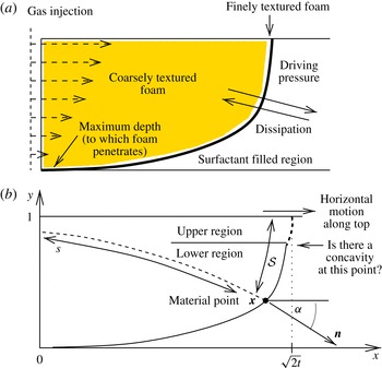
(a) Definition sketch for the pressure-driven growth model. Gas is injected into a reservoir flooded with surfactant solution. A front of finely textured foam forms at the boundary between gas and surfactant solution and is driven along by pressure, and retarded by dissipation. There is a maximum depth to which the front penetrates (obtained by balancing driving pressure with background hydrostatic pressure). (b) The foam front in
 $x$
,
 $y$
coordinates (assumed to be in dimensionless form here), such that at dimensionless time
 $t$
the leading edge at the top of the front is at
 $x=\sqrt{2t}$
. A material point is shown at vector location
 $\boldsymbol{x}$
, the distance it has moved is
 $s$
, and the distance along the front to reach it measured down from the top is
 ${\mathcal{S}}$
. The front normal
 $\boldsymbol{n}$
at the given point is at an angle
 $\unicode[STIX]{x1D6FC}$
from the horizontal. Motion along the top is horizontal, and the front can be divided into an upper region (which is influenced by this top boundary condition, and which grows in extent over time) and a lower region (which is unaffected by the top boundary condition, but which shrinks over time). One question to be addressed is whether or not there is a concave corner where there two regions meet.

The pressure-driven growth model, originally developed by Shan & Rossen (Reference Shan and Rossen2004) and discussed extensively by Grassia et al. (Reference Grassia, Mas-Hernández, Shokri, Cox, Mishuris and Rossen2014), is a way of computing the evolving front shape, which is sketched in figure 1. It considers that the front is propagating through a porous medium (i.e. the reservoir) and that the net pressure driving the front depends on the difference between the gas injection pressure and the background hydrostatic pressure in the reservoir, the latter growing with depth. As a result, the higher up a given point is on the foam front the faster and further it advances. It is relevant to ask whether, as the leading edge at the top of the foam front advances further and further over time, the portion of the reservoir that is left unswept continues to grow indefinitely (an undesirable situation known as gravity override (Shi & Rossen Reference Shi and Rossen1989; Boeije & Rossen Reference Boeije and Rossen2014)) or whether the area underneath the front that is left unswept approaches a well-defined limit even for very long times (i.e. override is avoided).
Insight into this issue can be obtained by studying asymptotic solutions of pressure-driven growth, applicable in different time regimes. An early time asymptotic solution for pressure-driven growth is available (de Velde Harsenhorst et al. Reference de Velde Harsenhorst, Dharma, Andrianov and Rossen2014) (‘early time’ in this context implies that the leading edge at the top of the front has travelled less distance than the maximum depth to which the front penetrates, this depth being reached when the background hydrostatic pressure balances the injection pressure). This early time solution clearly indicates that the amount of unswept reservoir beneath the foam front increases with time. If left unchecked indefinitely, this would produce gravity override. However, a late-time asymptotic solution is also available (Grassia et al. Reference Grassia, Mas-Hernández, Shokri, Cox, Mishuris and Rossen2014) (the top of the front has travelled much further than the maximum depth to which the front penetrates), and this indicates a finite amount of unswept area under the foam front.
Given the differing predictions at early and late times, it is relevant to ask how the early time solution gradually gives way to the late-time one. Better understanding of this can be obtained by noting some properties of the early and late-time solutions. Firstly the early time solution (de Velde Harsenhorst et al. Reference de Velde Harsenhorst, Dharma, Andrianov and Rossen2014) describes material points which have been continuously on the front since foam IOR began at time zero, and which have moved primarily horizontally, having been at (nearly) the same vertical height on the front throughout their entire time history to date. The late-time solution by contrast (Grassia et al. Reference Grassia, Mas-Hernández, Shokri, Cox, Mishuris and Rossen2014) describes material points which were not initially on the front, but which rather have spent the overwhelming majority of their history to date moving horizontally along the top boundary of the system, having then been ‘injected’ from the top boundary onto the front itself in the comparatively recent past: detailed discussion of this phenomenon is available in the literature (Grassia et al. Reference Grassia, Mas-Hernández, Shokri, Cox, Mishuris and Rossen2014).
As will be explained in more detail later, both the early time and late-time solutions have (in addition to a predominant horizontal motion) a downward vertical motion of material points superposed. Since material points do indeed migrate downwards, it follows then that the front is divided, at any given time, into a lower region (consisting of material points that have been continuously on the front since time zero) and an upper region (consisting of points that were initially on the top boundary and which have only been injected onto the front since time zero). In view of the downward motion of material points, over time, the vertical domain corresponding to the lower region shrinks, and that corresponding to the upper region grows. The early time asymptotic solution thus describes the lower region only, and does so at sufficiently short times when it accounts for the majority of the solution domain. Likewise the late-time asymptotic solution describes the upper region only, and does so at sufficiently long times when it likewise accounts for the majority of the solution domain.
Our concern here however is to determine the shape of the upper region at early times when it is still much smaller than the lower region (albeit growing). This is actually extremely important for computing the front shape numerically, particularly when using computational algorithms for pressure-driven growth that follow Lagrangian front material points. Such Lagrangian algorithms suffer from the fact these material points move ever further from the top boundary (Grassia et al. Reference Grassia, Mas-Hernández, Shokri, Cox, Mishuris and Rossen2014). Eventually it becomes necessary to regrid and add new material points close to the top boundary, but the question arises of where exactly they should be added (Grassia et al. Reference Grassia, Mas-Hernández, Shokri, Cox, Mishuris and Rossen2014). If one knew the front shape in the upper region exactly, one would know exactly where to add these new material points. However if one knew the front shape exactly, one would not be trying to compute it numerically!
Added to this dilemma is the issue that, if material points are placed incorrectly, it is possible to introduce artificial non-physical concavities into the front shape, which tend to evolve into concave sharp corners in pressure-driven growth: these require special handling in numerical schemes otherwise they produce spurious results (Grassia et al. Reference Grassia, Mas-Hernández, Shokri, Cox, Mishuris and Rossen2014; Mas-Hernández, Grassia & Shokri Reference Mas-Hernández, Grassia and Shokri2015a ,Reference Mas-Hernández, Grassia and Shokri b ). Indeed concavities have proved difficult to avoid in numerical computations (see e.g. figure 21 in Shan & Rossen (Reference Shan and Rossen2004)), which begs the question of whether the upper and lower regions might actually meet one another in a concave corner, despite the conventional hypothesis in the literature that the front shape in the present context should be wholly convex (Grassia et al. Reference Grassia, Mas-Hernández, Shokri, Cox, Mishuris and Rossen2014). This is one of the main questions which we will explore here.
The rest of this study is laid out as follows. In § 2 we discuss the pressure-driven growth model in more detail and give the relevant governing equations. In the first instance (§ 3) we analyse the lower region of the front, switching to analyse the upper region from § 4. Initially our upper region analyses are only approximate (§ 5), but in §§ 6 and 7 we offer improvements. Results are compared with a completely independent technique in § 8, with very favourable comparisons. Conclusions are outlined in § 9.
2 Pressure-driven growth
As we have said, the pressure-driven growth model (Shan & Rossen Reference Shan and Rossen2004; Grassia et al. Reference Grassia, Mas-Hernández, Shokri, Cox, Mishuris and Rossen2014) represents the shape of a foam front propagating through a porous medium, i.e. an oil reservoir during improved oil recovery. In what follows, before proceeding to describe the model itself, we first describe some features of the foam front propagation.
It is envisaged that first surfactant solution is injected into the reservoir and subsequently gas is injected under pressure, with a foam front being formed in situ at the boundary between surfactant and gas, and propagating along over time: see figure 1(a). The foam is formed on the pore scale in such a fashion that individual bubble films tend to span the pore cross-sections: these bubble films then restrict the ability of the injected gas to flow (Kovscek, Patzek & Radke Reference Kovscek, Patzek and Radke1997). Moreover the water saturation (i.e. the liquid fraction within the foam) is highest at the front (where the gas meets the surfactant solution) and is lower further upstream. Since wet foam is more stable than dry foam in this system (Kovscek et al. Reference Kovscek, Patzek and Radke1997), the so called texture of the foam (texture being measured either in terms of average bubble size, or equivalently in terms of number of bubble films per unit volume) is finer at the foam front and coarser upstream. It is assumed that there is an abrupt transition from fine texture to coarse texture as the foam dries out, such that the finely textured region becomes highly localised near the front (Shan & Rossen Reference Shan and Rossen2004). Given that the bubble films restrict the flow (as was already mentioned above) most of the resistance to flow through the porous medium comes from the wetter and hence more finely textured foam localised near the foam front, rather than from the drier and coarser foam upstream or indeed from the liquid surfactant solution downstream.
Darcy’s law for flow through a porous medium implies that the local velocity of flow is proportional to a pressure gradient, the coefficient of proportionality involving the ratio between the permeability of the medium and the viscosity of the fluid that is flowing. In the case of multiphase gas–liquid flow such as is being considered here, it is possible to define for each phase, a relative permeability and also an effective viscosity. What then governs the flow of each phase is neither the relative permeability nor the effective viscosity individually, but rather the ratio between them (Shan & Rossen Reference Shan and Rossen2004; Ma et al. Reference Ma, Ren, Mateen, Morel and Cordelier2015): we refer to this ratio as the relative mobility. In what is called a strong foam (such as the finely textured foam that appears at the front between injected gas and in situ surfactant solution), bubble films are so plentiful that there are no pathways for flow through the porous medium that do not involve crossing foam films. This means that the only way to mobilise gas is to mobilise bubble films also, a process which is highly dissipative. The relative mobility of the gas where the bubble films are most plentiful (i.e. in the finely textured foam at the foam front) is therefore exceedingly low. Having an exceedingly low mobility in a highly localised region at the foam front is the basis of the pressure-driven growth model, the physics of which we now describe in detail (§§ 2.1–2.2). Following that we present the governing equation for the pressure-driven growth model (§ 2.3), cast it in dimensionless form (§ 2.4), and discuss the nature of the model in general mathematical terms (§ 2.5).
2.1 Physical nature of pressure-driven growth
As alluded to above, Darcy’s law for flow in a porous medium describes flow down a gradient of pressure. However in a system for which the relative mobility of a particular phase is much lower in a restricted part of the flow domain than in any other part of the domain, almost all the loss in pressure is expected to occur across that low mobility zone. Indeed the pressure-driven growth model considers a limiting case (Shan & Rossen Reference Shan and Rossen2004) in which the entirety of the loss in pressure occurs across the neighbourhood of the foam front, the relative mobilities for gas in the coarsely textured foam upstream and for liquid in the surfactant solution downstream being assumed to be arbitrarily large compared to the relative mobility of gas in the finely textured foam at the front itself. Under these circumstances, all the non-trivial dynamics becomes focussed on the foam front itself: the foam front is pushed along by pressure, but is retarded by dissipation localised at the front, with pressure falling from a driving injection pressure upstream of the front to a background hydrostatic pressure downstream, the latter growing with depth. There is moreover a maximum depth to which the front can penetrate, corresponding to the depth at which the injection pressure is balanced by the hydrostatic pressure.
We are interested here, not just in the speed of foam front propagation, but also in the propagation direction. Since Darcy’s law describes flow down a pressure gradient, the direction of the flow necessarily matches the direction of the pressure gradient, which in the circumstances described above, must therefore be across the region of finely textured foam in the neighbourhood of the front (Shan & Rossen Reference Shan and Rossen2004). This implies the motion of the finely textured foam is normal to the front, i.e. the direction of propagation of the front is normal to the instantaneous front location. We consider that the gas is initially injected down a vertical injection well, so that the initial orientation of the front is vertical, and the initial propagation of the front is therefore horizontal. Nonetheless points higher up on the front propagate faster than those lower down, because the deeper one moves, the greater the hydrostatic pressure that opposes the pressure of gas injection. The front therefore reorients over time away from the vertical and propagation of the front thereby reorients away from the horizontal.
To give an idea of scale, in field applications, the foam front can over time (several days perhaps (Mas-Hernández et al. Reference Mas-Hernández, Grassia and Shokri2015a )), travel as much as several kilometres horizontally, penetrating several hundreds of metres below the surface (de Velde Harsenhorst et al. Reference de Velde Harsenhorst, Dharma, Andrianov and Rossen2014). In this work however, we shall focus on the comparatively early time evolution of the front, such that the horizontal displacement has still not managed to grow any larger than the penetration depth (i.e. several hundreds of metres). Meanwhile the zone of dissipative, finely textured foam at the foam front can be up to the order of a hundred metres thick, the thickness being measured along the direction of motion of the foam front (which is horizontal initially but which then reorients over time). The front thickness is rather less than either the penetration depth or the horizontal distance over which the front itself travels (Grassia et al. Reference Grassia, Mas-Hernández, Shokri, Cox, Mishuris and Rossen2014). Under these circumstances the front can be idealised in the first instance as being arbitrarily thin. The thickness of the dissipative, finely textured foam zone also tends to be less, the less the distance that the front has travelled (Shi Reference Shi1996; Shan & Rossen Reference Shan and Rossen2004): the implication is that the front initially moves quickly, but then slows down over time as the dissipation grows.
2.2 Physics excluded from pressure-driven growth
In addition to describing the physics included in the pressure-driven growth model, as was done above, it is also worth considering the physical effects that are excluded. This is done in what follows, and helps us to appreciate the possible limitations of the model.
The model treats gas in the finely textured foam as a fluid of low mobility, but considers the flow to be Newtonian. Foam is in actual fact a non-Newtonian fluid, so that the slower the motion of the gas in the region containing foam, the more its relative mobility should decrease. Typically the way that such non-Newtonian behaviour is modelled (Ma et al. Reference Ma, Ren, Mateen, Morel and Cordelier2015; Zeng et al. Reference Zeng, Muthuswamy, Ma, Wang, Farajzadeh, Puerto, Vincent-Bonnieu, Eftekhari, Wang and Da2016) is to suppose that there is a maximum possible mobility reduction (the maximum amount that the gas mobility is reduced in the presence of foam compared to the situation without foam) and this is achieved for gas moving at or below a certain given speed, defined in terms of a capillary number. If the gas moves more quickly than this given speed however, the extent to which the mobility is reduced becomes less. It is worth remembering that the pressure-driven growth model applies specifically to the case in which the mobility at the finely textured foam front is much less than the mobility elsewhere in the system (Grassia et al. Reference Grassia, Mas-Hernández, Shokri, Cox, Mishuris and Rossen2014). The pressure-driven growth model is therefore most likely to be applicable to systems in which the finely textured foam front experiences the maximum or close to the maximum mobility reduction. For this reason, within the pressure-driven growth model to be considered here, we choose to neglect the effect of non-Newtonian behaviour upon the mobility reduction. Another way of stating this is that we suppose that gas mobility is far more strongly affected by foam texture than by non-Newtonian effects, which is consistent with some of the cases considered in the study by Kovscek et al. (Reference Kovscek, Patzek and Radke1997).
Since the pressure-driven growth model relies so heavily upon having finely textured foam at the foam front, any effects that may compromise the integrity of that finely textured foam at the front may likewise impact upon the validity of the model. Although the model itself formally describes the process of surfactant alternating gas (i.e. gas injected into surfactant solution within a porous medium), the ultimate aim of the surfactant-alternating-gas process is to use foam to improve oil recovery. The presence of oil mixed with the surfactant solution might negatively affect the foam stability (see e.g. Farajzadeh et al. Reference Farajzadeh, Andrianov, Krastev, Hirasaki and Rossen2012; Osei-Bonsu, Shokri & Grassia Reference Osei-Bonsu, Shokri and Grassia2015, Reference Osei-Bonsu, Shokri and Grassia2016) and thereby influence the texture of the foam at the foam front. In addition to there being a requirement to maintain the integrity of the finely textured foam at the front itself, the validity of the model also demands that this finely textured foam be localised at the front (Shan & Rossen Reference Shan and Rossen2004). Failure of the foam to collapse abruptly and thereby coarsen as it dries out upstream, would affect the validity of the model in much the same fashion as oil destroying the integrity of the finely textured foam at the front.
Yet another aspect of the physics of foam in porous media that pressure-driven growth does not attempt to describe is the relative motion between liquid and gas within the foam. The model (Shan & Rossen Reference Shan and Rossen2004) does consider the gravity-induced hydrostatic pressure difference between liquid downstream of the foam front and gas upstream, but not any gravity-induced gas-to-liquid relative motion within the foam itself. Such relative motion within the foam with liquid draining downwards and gas rising upwards can lead to very low liquid content at the top of the foam. This dry out at the top makes the foam very coarsely textured and hence the gas mobility rises dramatically there. A tongue of highly mobile gas at the top of the system can then propagate above the liquid surfactant solution, far in advance of the remainder of the foam front which is much less mobile. This effect has been found by Kovscek et al. (Reference Kovscek, Patzek and Radke1997) to result in a concave corner forming at the point where the highly mobile tongue of gas meets the remainder of the front.
The pressure-driven growth model focusses attention solely on the finely textured low mobility zone at the foam front: therefore it is not designed to capture the aforementioned tongue of highly mobile gas at the top nor the concave corner that occurs where the tongue meets the rest of the front. Pressure-driven growth can however capture a related phenomenon associated with foam propagating into a surfactant solution with spatially non-uniform surfactant concentration, specifically with a lower surfactant concentration (and hence lower density) at the top, and a higher surfactant concentration (and hence higher density) lower down (Mas-Hernández et al. Reference Mas-Hernández, Grassia and Shokri2015a ). This again can lead to a concave corner in the foam front at the point where the lower surfactant concentration region (with less stable and hence less finely textured foam) meets the higher surfactant concentration region (with more stable and hence more finely textured foam). Our purpose in this work however is not to consider such systems with spatial non-uniformities in the foam texture measured along the front, but rather to investigate whether concave corners can occur even for foam fronts for which there is no variation in texture along the front itself: as we shall see later on, concave corners in front shape can develop even under these conditions.
Having now discussed the physics that the pressure-driven growth model includes, as well as the physics that it excludes, we proceed (in the next section) to introduce the governing equations for the model.
2.3 Governing equation for pressure-driven growth
The equation governing the pressure-driven growth model (Shan & Rossen Reference Shan and Rossen2004; Grassia et al.
Reference Grassia, Mas-Hernández, Shokri, Cox, Mishuris and Rossen2014) describes the motion of a material point
 $\boldsymbol{x}$
on the foam front via
 $$\begin{eqnarray}\frac{\text{d}\boldsymbol{x}}{\text{d}t}=\frac{k\unicode[STIX]{x1D706}_{r}}{(1-S_{w})\unicode[STIX]{x1D6F7}}\frac{\unicode[STIX]{x0394}P}{\unicode[STIX]{x1D70F}s}\boldsymbol{n},\end{eqnarray}$$
where
 $t$
is time,
 $\text{d}/\text{d}t$
represents a time derivative following a front material point,
 $\boldsymbol{n}$
is the front normal (which varies with distance
 ${\mathcal{S}}$
measured along the front, see figure 1(b)),
 $k$
is the permeability of the reservoir,
 $\unicode[STIX]{x1D706}_{r}$
is the relative mobility within the finely textured foam zone (relative mobility being the ratio between a relative permeability and an effective viscosity as already explained earlier),
 $S_{w}$
is the liquid fraction in the foam,
 $\unicode[STIX]{x1D6F7}$
is the reservoir porosity,
 $\unicode[STIX]{x0394}P$
is the driving pressure difference,
 $s$
is the distance the material point has travelled to date (again see figure 1
b),
 $\unicode[STIX]{x1D70F}$
(a small dimensionless parameter) is the ratio between the thickness of the finely textured foam front and the distance a material point has travelled: Grassia et al. (Reference Grassia, Mas-Hernández, Shokri, Cox, Mishuris and Rossen2014) employed a value
 $\unicode[STIX]{x1D70F}=0.01$
. As the distance
 $s$
through which the front has displaced grows, the thickness of the finely textured foam front
 $\unicode[STIX]{x1D70F}s$
likewise grows, and, since the dissipation is tied to the fine texture, the front slows down as a result. An additional slow down of the front over and above this could be incorporated into the governing equation due to non-Newtonian effects, but (for reasons already explained in § 2.2) such effects are neglected here.
The maximum depth to which the foam front can penetrate
 $d_{max}$
is given by balancing injection pressure with hydrostatic pressure and satisfies
 $$\begin{eqnarray}d_{max}=P_{inj}/(\unicode[STIX]{x0394}\unicode[STIX]{x1D70C}g),\end{eqnarray}$$
where
 $P_{inj}$
is the injection pressure,
 $\unicode[STIX]{x0394}\unicode[STIX]{x1D70C}$
is the liquid-to-gas density difference and
 $g$
is acceleration due to gravity.
We define our
 $x$
,
 $y$
coordinate system (figure 1
b) such that
 $x=0$
corresponds to the location of gas injection and
 $y=0$
corresponds to the maximum penetration depth. It follows that the net driving pressure (injection pressure less hydrostatic) grows linearly with coordinate
 $y$
 $$\begin{eqnarray}\unicode[STIX]{x0394}P=P_{inj}y/d_{max}.\end{eqnarray}$$
2.4 Dimensionless equations
We now make our governing equations dimensionless. Distances are non-dimensionalised on the scale
 $d_{max}$
, pressures are non-dimensionalised on the scale
 $P_{inj}$
and times are non-dimensionalised on the scale
 $$\begin{eqnarray}t_{scale}=\frac{(1-S_{w})\unicode[STIX]{x1D719}}{k\unicode[STIX]{x1D706}_{r}}\frac{d_{max}^{2}}{P_{inj}}\unicode[STIX]{x1D70F}.\end{eqnarray}$$
If we now use the symbols
 $\boldsymbol{x}$
,
 $s$
and
 $t$
to denote dimensionless (instead of dimensional) variables, we deduce the dimensionless analogue of (2.1)
 $$\begin{eqnarray}\frac{\text{d}\boldsymbol{x}}{\text{d}t}=\frac{y}{s}\boldsymbol{n}.\end{eqnarray}$$
Taking the dot product of this with
 $\boldsymbol{n}$
, it can be deduced that
 $s$
(the dimensionless path length over which the material point has travelled in dimensionless time
 $t$
) evolves according to
 $$\begin{eqnarray}\text{d}s/\text{d}t=y/s.\end{eqnarray}$$
These dimensionless equations must be solved with suitable initial and boundary conditions. Regarding initial conditions, at
 $t=0$
, we want the front to be at
 $x=0$
for all
 $y$
values in the solution domain, with additionally
 $s=0$
initially for all
 $y$
. This however predicts infinite
 $\text{d}\boldsymbol{x}/\text{d}t$
initially. In numerical computations, to avoid having infinite velocities initially, typically we put the front at some location
 $x=s_{0}$
(where
 $s_{0}$
is a dimensionless parameter much smaller than unity) with in addition
 $s=s_{0}$
initially. Typically
 $s_{0}$
is chosen (Grassia et al.
Reference Grassia, Mas-Hernández, Shokri, Cox, Mishuris and Rossen2014) with a value of the order of 10
 $^{-2}$
. Regarding boundary conditions, at the top of the solution domain
 $y=1$
, we require that the front material points move parallel to the top boundary: in other words the normal
 $\boldsymbol{n}$
is horizontal at that point. Suppose we use the symbol
 $\unicode[STIX]{x1D6FC}$
(as sketched in figure 1
b) to denote the angle that the normal makes to the horizontal at any point on the front. By definition
 $$\begin{eqnarray}\unicode[STIX]{x1D6FC}\equiv \arctan (\text{d}x/\text{d}y),\end{eqnarray}$$
where
 $\text{d}/\text{d}y$
denotes a spatial derivative with respect to vertical location along the foam front at any given instant in time (a contrast from
 $\text{d}/\text{d}t$
which denotes the motion of material points on trajectories that are normal to the instantaneous foam front). In view of (2.7), another way of writing the top boundary condition is as
 $\unicode[STIX]{x1D6FC}=0$
at
 $y=1$
.
Corroborating a claim made back in § 2.1, one thing we immediately notice here based on (2.5)–(2.6) is that points higher up advance faster and hence further than points lower down. The conventional hypothesis in the literature is that this leads to a convex front shape as seen from downstream (Grassia et al. Reference Grassia, Mas-Hernández, Shokri, Cox, Mishuris and Rossen2014; Mas-Hernández et al. Reference Mas-Hernández, Grassia and Shokri2015a ,Reference Mas-Hernández, Grassia and Shokri b ). One of our aims here is to investigate whether that conventional hypothesis is correct, or whether the shape might admit a concavity. The role that concavities can play from a mathematical point of view is described in the next section.
2.5 Mathematical nature of pressure-driven growth and the behaviour of concavities
In order to understand the possible significance of concavities in pressure-driven growth, it is useful to consider the nature of the model in general mathematical terms.
A key mathematical feature of pressure-driven growth is that it assigns no energy cost to the overall length of the front, meaning that the solutions can admit some really quite unusual front shapes, including shapes containing various types of singularities. In particular it is known that concave regions in a front tend to focus down into corners which are ‘arbitrarily’ sharp (‘arbitrarily’ sharp in the current context implying a radius of curvature comparable with the thickness of the dissipative, finely textured foam zone, which is much less than the distance over which the front travels (Grassia et al. Reference Grassia, Mas-Hernández, Shokri, Cox, Mishuris and Rossen2014)). The fact that singularities can arise within solutions of pressure-driven growth is unsurprising because a formal equivalence has been proven (Grassia et al. Reference Grassia, Mas-Hernández, Shokri, Cox, Mishuris and Rossen2014) between pressure-driven growth and another equation that admits singularities, namely the eikonal equation, a well-known hyperbolic partial differential equation originally formulated in the context of optics (Arnold Reference Arnold2004).
Returning to consider the case of pressure-driven growth, when a Lagrangian scheme is used to evolve the front location, any concave corners that occur need to be propagated differently from surrounding front material points (Grassia et al. Reference Grassia, Mas-Hernández, Shokri, Cox, Mishuris and Rossen2014; Mas-Hernández et al. Reference Mas-Hernández, Grassia and Shokri2015a ,Reference Mas-Hernández, Grassia and Shokri b ). In such numerical schemes, the consequences of not propagating the concave corners correctly are very serious indeed: segments of the front cross-over one another, forming topologically infeasible spurious loops in the representation of the front, and these spurious loops then grow indefinitely (Grassia et al. Reference Grassia, Mas-Hernández, Shokri, Cox, Mishuris and Rossen2014).
These issues should not arise of course for a wholly convex front. If concavities do nevertheless appear in a computed foam front shape, we can draw one of two conclusions: either a numerical scheme has artificially introduced a concavity where one is not supposed to be, or else the foam front really does have a concavity according to the underlying model.
It is explained by Grassia et al. (Reference Grassia, Mas-Hernández, Shokri, Cox, Mishuris and Rossen2014) that it is relatively easy to introduce a concavity inadvertently in a numerical scheme designed to track Lagrangian material points on a foam front: particularly when one is adding new material points in the process of regridding a numerical representation of the front, such regridding needing to occur from time to time whenever material points are separating from one another. If the new material point is placed too far back, a concavity is created at the newly placed point itself. On the other hand, if the new material point is placed too far forward, a concavity is created above or below the point (or both). The problem is particularly acute on any parts of the front where the front curvature happens to be low: since then the set of locations within which new material points can be safely placed is very limited indeed.
If, even in spite of best efforts to place newly added numerical points in such a way as to avoid artificially introducing concavities, it still turns out that concavities manage to arise, the question then arises as to whether the concavities might actually be an inherent part of the front shape. This is the question we wish to explore here, employing asymptotic rather than numerical techniques (in order to be confident that any predictions we make are not simply numerical artefacts associated with Lagrangian schemes as described above).
3 Front shape in the lower region
An asymptotic solution for the foam front, valid for early times
 $t\ll 1$
, has been proposed by de Velde Harsenhorst and co-workers (de Velde Harsenhorst et al.
Reference de Velde Harsenhorst, Dharma, Andrianov and Rossen2014). In what follows we call this the Velde solution, and we briefly outline its derivation below (§ 3.1). After that (going beyond the analysis of de Velde Harsenhorst et al. (Reference de Velde Harsenhorst, Dharma, Andrianov and Rossen2014)) we demonstrate that the Velde solution is only valid in part of the solution domain, specifically in the ‘lower region’ of the domain (§ 3.2). We also show how to improve upon the Velde solution (§§ 3.3–3.4): as we will see, such improved solutions also help to give us an indication of the time limits of validity of the original Velde
 $t\ll 1$
solution, so that even for times as large as
 $t=0.5$
the relative error in the Velde solution is only a few per cent.
3.1 Derivation of the Velde solution
Recall that in the situation under consideration here, gas is injected into surfactant solution initially along a vertical injection well, so that the foam front is initially vertical and its normal is initially horizontal. Although the direction of the front normal does not remain horizontal at all times, the Velde solution recognises that at sufficiently early times, the front normal will point nearly horizontally and the front motion is primarily horizontal with only a small vertical component superposed.
The
 $x$
component of (2.5) can be written
 $$\begin{eqnarray}\frac{\text{d}x}{\text{d}t}=\frac{y}{s}\cos \unicode[STIX]{x1D6FC},\end{eqnarray}$$
where we recall that
 $\text{d}/\text{d}t$
denotes a time derivative following a material point (a contrast from the notation
 $\text{d}/\text{d}y$
, which denotes a spatial derivative with respect to vertical location along the foam front from material point to material point). Since for nearly horizontal motion,
 $s$
is nearly the same as
 $x$
and
 $\cos \unicode[STIX]{x1D6FC}$
is close to unity, it follows from (3.1) that
 $$\begin{eqnarray}x\approx \sqrt{2yt},\end{eqnarray}$$
where the temporal variation of
 $y$
has been ignored with respect to that of
 $x$
. Equivalently
 $$\begin{eqnarray}y\approx \frac{x^{2}}{2t},\end{eqnarray}$$
showing that the predicted front shape is a parabola. This parabolic shape relies on the fact that gas is injected initially over the entire vertical depth of the front: if gas had not been injected over the entire vertical line but instead over a much more localised region as has been considered by Kovscek et al. (Reference Kovscek, Patzek and Radke1997), rather different front shapes then result.
The Velde solution (3.2) whilst undoubtedly useful has a number of issues. Firstly, since it implies
 $$\begin{eqnarray}\frac{\text{d}x}{\text{d}y}\approx \sqrt{\frac{t}{2y}}\end{eqnarray}$$
but assumes a nearly vertical front, i.e.
 $\text{d}x/\text{d}y\ll 1$
, it requires
 $y\gg t/2$
. Under these conditions (combining (3.4) with (2.7)) we find
 $$\begin{eqnarray}\unicode[STIX]{x1D6FC}\approx \frac{\text{d}x}{\text{d}y}\approx \sqrt{\frac{t}{2y}}\ll 1.\end{eqnarray}$$
This is however invalid for small
 $y$
values of order
 $t/2$
or less, but this is actually not problematic for computing how the front shape evolves. We are dealing with
 $t\ll 1$
here, and hence
 $y$
must be exceedingly small if it is of order
 $t/2$
or less: there is little net front motion as
 $y\rightarrow 0$
anyway, because driving pressure and background hydrostatic pressure are nearly in balance.
Determining what is happening near the top of the front
 $y=1$
is more problematic. Although the Velde solution (3.2) gives the correct
 $x$
value for material points moving along the top boundary
 $x=\sqrt{2t}$
, it gives a value of
 $\text{d}x/\text{d}y$
at the top equal to
 $\sqrt{t/2}$
. We are assuming that
 $t\ll 1$
here, so
 $\sqrt{t/2}$
is a small parameter, but nonetheless it differs from zero, despite the fact that the boundary condition at the top requires that it should be zero. The explanation why the top boundary condition is not satisfied by the Velde solution is considered below.
3.2 Vertical motion predicted by the Velde solution
The reason why the Velde solution (3.2) is problematic near the top boundary can be seen by examining the vertical motion of material points. The
 $y$
component of (2.5) is
 $$\begin{eqnarray}\frac{\text{d}y}{\text{d}t}=-\frac{y}{s}\sin \unicode[STIX]{x1D6FC}.\end{eqnarray}$$
Since in the regime of interest,
 $s\approx x$
and
 $\sin \unicode[STIX]{x1D6FC}\approx \tan \unicode[STIX]{x1D6FC}\equiv \text{d}x/\text{d}y$
, it follows using (3.2) and (3.4) that
 $$\begin{eqnarray}\text{d}y/\text{d}t\approx -1/2\end{eqnarray}$$
uniformly for all
 $y$
. In other words, any material points to which the Velde solution applies also obey (3.7) and hence by time
 $t$
invariably find themselves at
 $y$
values below
 $1-t/2$
.
Thus the Velde solution is only valid in the lower region of the solution domain, namely for
 $y<1-t/2$
. In the upper region, i.e. in the domain
 $1-t/2\leqslant y\leqslant 1$
, a different solution must be found, and this solution must meet the boundary condition that
 $\unicode[STIX]{x1D6FC}=0$
on the top boundary. We will analyse the upper region of the solution domain in § 4, but before doing that, we wish to consider the consequences that (3.7) implies for the lower region.
3.3 Improving the Velde solution
Equation (3.7) makes it possible to improve upon the Velde solution (3.2), which was originally based on the assumption of constant rather than variable
 $y$
. In what follows, the improvement to the Velde solution is derived: those readers who wish to skip the derivation should turn directly to (3.13)–(3.14) and the results in § 3.3.1. The derivation that we follow is similar to one that has already been employed by Grassia (Reference Grassia2017) to describe pressure-driven growth within porous media with anisotropic permeability. Here the system is considered to be isotropic, and there are some subtle (albeit significant) differences in the equations obtained: see Grassia (Reference Grassia2017) for details.
The improvement to the Velde solution can be obtained starting from (2.5) by recognising that
 $s$
at any instant is slightly larger than
 $x$
(owing to the vertical component of motion being superposed upon the horizontal component), that
 $\cos \unicode[STIX]{x1D6FC}$
is well approximated by
 $1-\unicode[STIX]{x1D6FC}^{2}/2$
, and also that historical values of
 $y$
for any given material point were slightly larger than the current values.
Specifically
 $$\begin{eqnarray}s=\int _{0}^{x}\left(1+\frac{({\dot{y}})^{2}}{({\dot{x}})^{2}}\right)^{1/2}\,\text{d}x\approx \int _{0}^{x}\left(1+\frac{1}{2}\frac{({\dot{y}})^{2}}{({\dot{x}})^{2}}\right)\,\text{d}x,\end{eqnarray}$$
where
 ${\dot{x}}$
and
 ${\dot{y}}$
are shorthand for time derivatives. If we substitute
 ${\dot{x}}$
from the Velde solution (3.2), replace
 $\text{d}x$
by
 ${\dot{x}}\,\text{d}t$
, set
 ${\dot{y}}\approx -1/2$
and integrate, we deduce
 $$\begin{eqnarray}s\approx x(1+t/(12y)).\end{eqnarray}$$
It follows (for small
 $t$
)
 $$\begin{eqnarray}s^{-1}\approx x^{-1}(1-t/(12y)).\end{eqnarray}$$
Meanwhile
 $$\begin{eqnarray}\cos \unicode[STIX]{x1D6FC}\approx 1-\frac{\unicode[STIX]{x1D6FC}^{2}}{2}\approx 1-\frac{(\text{d}x/\text{d}y)^{2}}{2}\approx 1-\frac{t}{4y},\end{eqnarray}$$
where (3.4) has been used. Additionally, if a material point is at location
 $y$
at time
 $t$
, then, at some earlier time
 $t^{\prime }$
, its location must have been
 $y+(t-t^{\prime })/2$
or equivalently
 $y(1+(t-t^{\prime })/(2y))$
.
Substituting the above into (3.1) it follows
 $$\begin{eqnarray}x\approx \sqrt{2y\int _{0}^{t}(1-t^{\prime }/(12y))(1+(t-t^{\prime })/(2y))(1-t^{\prime }/(4y))\,\text{d}t^{\prime }}.\end{eqnarray}$$
Performing the integrals, retaining only terms through to order
 $t^{2}$
(discarding any higher powers of
 $t$
) we deduce
 $$\begin{eqnarray}x\approx \sqrt{2yt+t^{2}/6}.\end{eqnarray}$$
Equation (3.13) can be viewed as a correction or improvement to the Velde solution incorporating contributions to
 $x$
at order
 $t^{3/2}$
over and above the leading-order term
 $\sqrt{2yt}$
. It is clear that (at any given
 $y$
) the value of
 $x$
according to (3.13) is slightly larger than what is predicted by the Velde solution (3.2). In other words the front is displaced to the right, i.e. it travels slightly further than the Velde solution predicts, benefitting from the fact that historically material points were moving more rapidly having been higher up than their current
 $y$
location.
Equivalent to (3.13) we can write
 $$\begin{eqnarray}y\approx \frac{x^{2}}{2t}-\frac{t}{12},\end{eqnarray}$$
which predicts that the ‘improved’ Velde solution is a vertical distance
 $t/12$
below the original given by (3.3) regardless of the value of
 $x$
. As a result there is less unswept area underneath the front (i.e. less gravity override) with the ‘improved’ Velde solution (3.13) than with the original (3.2). Rearranging (3.2) to obtain (3.3), and integrating equation (3.3) from
 $x=0$
to the leading edge of the front at
 $x=\sqrt{2t}$
, we deduce the unswept area under the original Velde solution to be
 $\sqrt{2t}/3$
. The improvement to the Velde solution (i.e. (3.14) obtained from (3.13)) however reduces this unswept area by an amount
 $\sqrt{2}t^{3/2}/12$
, thereby helping to arrest the growth in unswept area and limit the override.
3.3.1 Comparison with simulation data
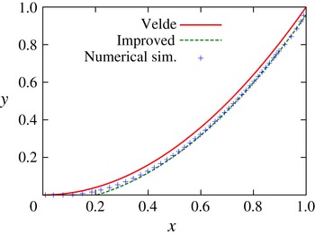
In figure 2 we have compared the prediction of (3.13) with a numerically simulated foam front, all results corresponding to a time
 $t=0.5$
. These numerical simulations were performed using the same algorithm for computing the trajectories of Lagrangian material points as described in detail in Grassia et al. (Reference Grassia, Mas-Hernández, Shokri, Cox, Mishuris and Rossen2014). The simulations used 40 material points initially (albeit with additional material points being added over time as points separate from one another, there being 46 material points in total by time
 $t=0.5$
) and a time step of
 $5\times 10^{-5}$
.


At time
 $t=0.5$
, the error in vertical position between the ‘original’ Velde solution (3.3) and the ‘improved’ solution (3.14) is
 $t/12\approx 0.04$
. Considering that
 $y$
varies between 0 and 1 here, the difference between the ‘original’ and ‘improved’ Velde solutions is still small in relative terms, even for
 $t=0.5$
. Nonetheless it is clear that the numerical simulation data in figure 2 agree much better with the ‘improved’ Velde solution (3.13) than with the original Velde solution (3.2). Indeed, given that the ‘improved’ Velde solution is formally a
 $t\ll 1$
solution, it is remarkable that it agrees so well with
 $t=0.5$
numerical data. Nonetheless it is clear that the ‘improved’ solution still only applies in the lower region of the solution domain. Equation (3.13) is seen to deviate from the numerical simulation data in the upper region of the domain as
 $y\rightarrow 1$
. It is not so much a case of (3.13) ceasing to be a valid solution for pressure-driven growth per se, but instead a case of the upper region being influenced by a top boundary condition which (3.13) fails to respect. Not only does (3.13) fail to give
 $\text{d}x/\text{d}y\rightarrow 0$
in the limit as
 $y\rightarrow 1$
, it also gives the wrong value of
 $x$
, predicting
 $x\approx \sqrt{2t+t^{2}/6}$
in this limit, instead of the correct value
 $x=\sqrt{2t}$
.
3.4 Improved estimate of vertical motion
Having obtained an improved estimate of the displacement in the
 $x$
direction (via (3.13)) and having demonstrated in § 3.3.1 that it really does fit the front shape better, we can now proceed to obtain an improved estimate of the trajectory of
 $y$
versus
 $t$
. A derivation follows, but some readers may wish to skip to the final result in (3.23).
We start by considering (2.6), and note that on the right-hand side we can replace
 $y$
to a good approximation by the following
 $$\begin{eqnarray}y\approx y_{0}-t/2,\end{eqnarray}$$
where
 $y_{0}$
is the initial location of the material point currently at
 $y$
. Upon integrating (2.6) and Taylor expanding for small
 $t$
 $$\begin{eqnarray}s\approx \sqrt{2y_{0}t-\frac{t^{2}}{2}}\approx \sqrt{2y_{0}t}\left(1-\frac{t}{8y_{0}}\right)\end{eqnarray}$$
and hence
 $$\begin{eqnarray}\frac{1}{s}\approx \frac{1}{\sqrt{2y_{0}t}}\left(1+\frac{t}{8y_{0}}\right).\end{eqnarray}$$
Via (3.13)
 $$\begin{eqnarray}\frac{\text{d}x}{\text{d}y}\approx \frac{t}{\sqrt{2yt+t^{2}/6}}.\end{eqnarray}$$
Substituting from (3.15) and Taylor expanding for small
 $t$
it follows
 $$\begin{eqnarray}\frac{\text{d}x}{\text{d}y}\approx \sqrt{\frac{t}{2y_{0}}}\left(1+\frac{5t}{24y_{0}}\right).\end{eqnarray}$$
Moreover (again via a Taylor expansion)
 $$\begin{eqnarray}\sin \unicode[STIX]{x1D6FC}=\sin \left(\arctan \frac{\text{d}x}{\text{d}y}\right)\approx \frac{\text{d}x}{\text{d}y}-\frac{1}{2}\left(\frac{\text{d}x}{\text{d}y}\right)^{3}.\end{eqnarray}$$
Upon substituting from (3.19) and expanding for small
 $t$
 $$\begin{eqnarray}\sin \unicode[STIX]{x1D6FC}\approx \sqrt{\frac{t}{2y_{0}}}\left(1-\frac{t}{24y_{0}}\right).\end{eqnarray}$$
Substituting (3.15), (3.17) and (3.21) into (3.6)
 $$\begin{eqnarray}y-y_{0}\approx -\frac{1}{2y_{0}}\int _{0}^{t}(1+t^{\prime }/(8y_{0}))(y_{0}-t^{\prime }/2)(1-t^{\prime }/(24y_{0}))\,\text{d}t^{\prime }.\end{eqnarray}$$
Integrating, whilst discarding any terms higher than order
 $t^{2}$
, gives
 $$\begin{eqnarray}y\approx y_{0}-\frac{t}{2}+\frac{5t^{2}}{48y_{0}},\end{eqnarray}$$
where
 $y_{0}\leqslant 1$
is the material point’s initial location.
This equation indicates that material points actually migrate downward slightly slower than speed
 $1/2$
(a point we will return to much later on in § 8), the main contributing effect being that the net driving pressure (injection pressure less hydrostatic pressure) decays as points move downwards. Nonetheless material points still do migrate downwards, so the improvements to the Velde solution that we have presented here cannot apply all the way up to
 $y=1$
for any finite
 $t>0$
: that requires a different analysis as we now consider.
4 Front shape in the upper region
Having discussed how the early time solution behaves in the lower region (material points which have been continuously on the front since time zero), we now turn to consider early time solution for the upper region (material points injected onto the front from the top boundary after time zero).
A description of the shape of the upper region of the foam front at early times is equivalent to describing how the orientation of the front (represented by an angle
 $\unicode[STIX]{x1D6FC}$
, specifically the orientation of the front normal with respect the horizontal) depends on the location
 $1-y$
(the vertical distance measured down from the top of the front). In the upper region of the front at early times, two small distances are relevant:
 $1-y$
(as mentioned above) and the vertical distance from the top boundary to the matching point with the lower region (which is expected to be approximately
 $t/2$
, at least based on the behaviour observed in the lower region). We shall look in the first instance for a similarity solution which depends on the ratio between these two small distances. In what follows we consider, in the upper region, how material elements on the foam front rotate over time (§ 4.1), and also how they move downwards over time (§ 4.2), finally relating the change in orientation to the change in vertical position to deduce a governing equation for the front shape (§ 4.3).
4.1 Rotation rate of material elements
In this section, an equation (namely (4.4)) for the rotation rate of material elements is derived. One of the key questions that we wish to address in this work is whether or not this equation for the rotation rate can be replaced by a slightly simpler equation, namely (4.5). The relevant derivations follow.
Material elements rotate due to non-uniformities in the speed of material points from place to place. It follows then that the rotation rate of a material element
 $\dot{\unicode[STIX]{x1D6FC}}$
depends on how the material point speed varies with arc length measured along the front, i.e.
 $$\begin{eqnarray}\dot{\unicode[STIX]{x1D6FC}}=-\frac{\text{d}}{\text{d}{\mathcal{S}}}\left(\frac{y}{s}\right).\end{eqnarray}$$
Here
 $y/s$
is the material point speed according to (2.6) (
 $y$
is vertical coordinate,
 $s$
is distance measured along the trajectory). Moreover
 ${\mathcal{S}}$
is distance measured along the front (in the downwards direction).
We can expand this as follows
 $$\begin{eqnarray}\dot{\unicode[STIX]{x1D6FC}}=-\frac{1}{s}\frac{\text{d}y}{\text{d}{\mathcal{S}}}+\frac{y}{s^{2}}\frac{\text{d}s}{\text{d}y}\frac{\text{d}y}{\text{d}{\mathcal{S}}}.\end{eqnarray}$$
Since
 $\text{d}y/\text{d}{\mathcal{S}}=-\text{cos}\,\unicode[STIX]{x1D6FC}$
(by definition) we deduce
 $$\begin{eqnarray}\dot{\unicode[STIX]{x1D6FC}}=\frac{\cos \unicode[STIX]{x1D6FC}}{s}\left(1-\frac{y}{s}\frac{\text{d}s}{\text{d}y}\right).\end{eqnarray}$$
At small times and near the top boundary,
 $\cos \unicode[STIX]{x1D6FC}\approx 1$
,
 $s\approx \sqrt{2t}$
,
 $y\approx 1$
and hence,
 $$\begin{eqnarray}\dot{\unicode[STIX]{x1D6FC}}\approx \frac{1}{\sqrt{2t}}\left(1-\frac{1}{\sqrt{2t}}\frac{\text{d}s}{\text{d}y}\right).\end{eqnarray}$$
At early times we know that
 $s$
is well approximated by
 $x$
: being able to replace
 $s$
by
 $x$
is a significant simplification as
 $s$
is history dependent, but
 $x$
depends only on instantaneous location of a material point. It is valid to ask whether in the above formula for
 $\dot{\unicode[STIX]{x1D6FC}}$
we can then replace
 $\text{d}s/\text{d}y$
by
 $\text{d}x/\text{d}y$
(the latter being
 $\tan \unicode[STIX]{x1D6FC}$
, which is essentially the same as
 $\unicode[STIX]{x1D6FC}$
at small times when
 $\unicode[STIX]{x1D6FC}$
is invariably small). The difficulty is that near the top boundary
 $\text{d}x/\text{d}y$
vanishes, so (even though
 $x$
and
 $s$
are close), it is not a priori clear whether
 $\text{d}x/\text{d}y$
and
 $\text{d}s/\text{d}y$
are actually similar in magnitude or not.
Suppose that it is possible to make this replacement. Then
 $$\begin{eqnarray}\dot{\unicode[STIX]{x1D6FC}}\sim \frac{1}{\sqrt{2t}}\left(1-\frac{1}{\sqrt{2t}}\,\frac{\text{d}x}{\text{d}y}\right)\approx \frac{1}{\sqrt{2t}}\left(1-\frac{\unicode[STIX]{x1D6FC}}{\sqrt{2t}}\right).\end{eqnarray}$$
At the top boundary,
 $\unicode[STIX]{x1D6FC}\rightarrow 0$
, so
 $\dot{\unicode[STIX]{x1D6FC}}\approx 1/\sqrt{2t}$
regardless of whether (4.4) or (4.5) is used. Below the top boundary however, the solution for
 $x$
versus
 $y$
might be expected to match onto the lower part of the solution domain, where the Velde solution
 $x\approx \sqrt{2yt}$
as given by (3.2) should be (approximately) valid. The matching point is expected to occur somewhere near
 $y\approx 1-t/2$
(with
 $t$
being chosen much smaller than unity here). This implies that
 $\unicode[STIX]{x1D6FC}\approx \text{d}x/\text{d}y\approx \sqrt{t/(2y)}$
according to (3.4), which for
 $y$
values close to unity (i.e. for
 $1-y\ll 1$
) becomes
 $\unicode[STIX]{x1D6FC}\approx \sqrt{t/2}$
. Hence (according to (4.5) and assuming
 $\unicode[STIX]{x1D6FC}$
is a continuous function moving between the upper and lower regions) at the matching point, we must have
 $\dot{\unicode[STIX]{x1D6FC}}\approx 1/(2\sqrt{2t})$
, which is only half as big as
 $\dot{\unicode[STIX]{x1D6FC}}$
at the top boundary. It would appear that there are significant spatio-temporal non-uniformities in
 $\dot{\unicode[STIX]{x1D6FC}}$
across a comparatively small domain.
4.2 Vertical motion of material elements
According to the pressure-driven growth model, the vertical motion of material elements is as per (3.6). Since in the upper region we are interested in
 $y$
values near unity,
 $s$
values roughly
 $\sqrt{2t}$
, and
 $\unicode[STIX]{x1D6FC}$
much smaller than unity it follows
 $$\begin{eqnarray}{\dot{y}}\approx -\unicode[STIX]{x1D6FC}/\sqrt{2t}.\end{eqnarray}$$
Note this is apparently consistent with the foregoing analysis for the lower region discussed in § 3. The matching point with the Velde solution, should be close to
 $y=1$
when
 $t\ll 1$
, and is expected to satisfy
 $\unicode[STIX]{x1D6FC}\approx \sqrt{t/2}$
, at least under the assumption that the upper and lower regions are to join up with the same orientation (in which case (3.4) can be applied where the regions join). It then follows
 ${\dot{y}}\approx -1/2$
, and hence, on the basis of this assumption, the matching point is therefore predicted to be approximately a distance
 $t/2$
below the top boundary.
What we have demonstrated here is that, if the upper and lower regions match up with the same front orientation, then the vertical velocity component of the uppermost material point of the lower region is the same as the vertical velocity component of the lowermost material point of the upper region. Given these two material points are initially adjacent, if their subsequent vertical velocity components are also the same, then they must remain adjacent to one another as time proceeds. Under these circumstances, the matching point is (by definition) precisely where these two material points meet, and it too must move downwards with the same velocity component as the material points themselves do.
What we have not ruled out of course is a more complicated case where the upper and lower regions join up with different front orientations e.g. in a concave corner. It is known in the literature for instance that concave corners can consume material points (Grassia et al. Reference Grassia, Mas-Hernández, Shokri, Cox, Mishuris and Rossen2014). Thus the material points either side of a concave corner at any given time are not necessarily the same as those either side of that concave corner at any other time. It follows then that the downward motion of the concave corner need not match that of material points either, since the identities of the material points immediately adjacent to either side of the corner are continually changing.
As we will see (in §§ 6–7), it is absolutely essential to consider this more complicated situation for a proper understanding of the shape of the foam front. For the present however, we wish to explore the consequences of assuming the simpler situation for which the upper and lower regions match with the same front orientation. Ultimately this assumption will lead us towards a contradiction (see § 5), but the analysis we perform here is nonetheless useful, as it is amenable to be generalised to the more complex situations in §§ 6–7.
4.3 Proposed similarity solution for front shape and its governing equation
In this section, we propose a similarity solution for the front shape, and derive a governing equation for that similarity solution. The derivation follows, but some readers may prefer to skip directly to the result given in (4.17).
We begin by defining a similarity variable
 $$\begin{eqnarray}\unicode[STIX]{x1D701}=(1-y)/(t/2),\end{eqnarray}$$
with
 $\unicode[STIX]{x1D701}=0$
at the top boundary (
 $y=1$
) and
 $\unicode[STIX]{x1D701}=1$
at the expected location of the matching point (
 $y=1-t/2$
). Clearly
 $\unicode[STIX]{x1D701}$
represents a ratio of distances, i.e. the ratio between the distance that a point
 $y$
is below the top surface, and the (assumed) distance between the top surface and the matching point itself.
We now look for a similarity solution in the small-time limit assumed to take the form
 $$\begin{eqnarray}\unicode[STIX]{x1D6FC}=\sqrt{t/2}A(\unicode[STIX]{x1D701}),\end{eqnarray}$$
where
 $A(\unicode[STIX]{x1D701})$
is a function that we must determine. Matching onto the top boundary requires
 $A=0$
when
 $\unicode[STIX]{x1D701}=0$
and matching onto the lower region (assuming continuity of
 $\unicode[STIX]{x1D6FC}$
and hence of
 $A$
) implies
 $A=1$
when
 $\unicode[STIX]{x1D701}=1$
. Note the geometrical interpretation of this: the larger the value of
 $A$
(and hence of
 $\unicode[STIX]{x1D6FC}$
for any given time
 $t$
) the greater the extent to which a material element on the front has reoriented compared to the orientation at the top boundary, and hence the greater the curvature of the front.
Our aim here is to obtain a differential equation determining
 $A$
as a function of
 $\unicode[STIX]{x1D701}$
. The proposed similarity form given in (4.8) not only governs how
 $\unicode[STIX]{x1D6FC}$
varies with position on the front at fixed time
 $t$
, but also how
 $\unicode[STIX]{x1D6FC}$
and vertical position evolve with time following a specified material point. Taking a time derivative following a material point of the expression (4.7) for
 $\unicode[STIX]{x1D701}$
gives
 $$\begin{eqnarray}\dot{\unicode[STIX]{x1D701}}=-\frac{{\dot{y}}}{t/2}-\unicode[STIX]{x1D701}/t.\end{eqnarray}$$
Since via (4.6) (applicable in the small-time limit) and (4.8)
 $$\begin{eqnarray}{\dot{y}}\approx -\unicode[STIX]{x1D6FC}/\sqrt{2t}\approx -A/2,\end{eqnarray}$$
it follows
 $$\begin{eqnarray}\dot{\unicode[STIX]{x1D701}}\approx (A-\unicode[STIX]{x1D701})/t.\end{eqnarray}$$
We can also differentiate the expression (4.8) for
 $\unicode[STIX]{x1D6FC}$
with respect to time (at fixed
 $y$
)
 $$\begin{eqnarray}\unicode[STIX]{x2202}\unicode[STIX]{x1D6FC}/\unicode[STIX]{x2202}t=1/(2t)\unicode[STIX]{x1D6FC}+\sqrt{t/2}(-\unicode[STIX]{x1D701}/t)A_{\unicode[STIX]{x1D701}}=\sqrt{t/2}A/(2t)+\sqrt{t/2}(-\unicode[STIX]{x1D701}/t)A_{\unicode[STIX]{x1D701}},\end{eqnarray}$$
where
 $A_{\unicode[STIX]{x1D701}}$
denotes the derivative of
 $A$
with respect to
 $\unicode[STIX]{x1D701}$
. Meanwhile
 $$\begin{eqnarray}\unicode[STIX]{x2202}\unicode[STIX]{x1D6FC}/\unicode[STIX]{x2202}y=-\sqrt{t/2}A_{\unicode[STIX]{x1D701}}/(t/2)\end{eqnarray}$$
and moreover (using (4.10))
 $$\begin{eqnarray}{\dot{y}}\unicode[STIX]{x2202}\unicode[STIX]{x1D6FC}/\unicode[STIX]{x2202}y\approx \sqrt{t/2}AA_{\unicode[STIX]{x1D701}}/t.\end{eqnarray}$$
Summing
 $\unicode[STIX]{x2202}\unicode[STIX]{x1D6FC}/\unicode[STIX]{x2202}t$
and
 ${\dot{y}}\unicode[STIX]{x2202}\unicode[STIX]{x1D6FC}/\unicode[STIX]{x2202}y$
we deduce for the rate of change of
 $\unicode[STIX]{x1D6FC}$
following a material point
 $$\begin{eqnarray}\dot{\unicode[STIX]{x1D6FC}}\approx \sqrt{t/2}A/(2t)+\sqrt{t/2}(A-\unicode[STIX]{x1D701})A_{\unicode[STIX]{x1D701}}/t.\end{eqnarray}$$
We now equate this to
 $\dot{\unicode[STIX]{x1D6FC}}\sim (\sqrt{2t})^{-1}(1-\unicode[STIX]{x1D6FC}/\sqrt{2t})$
(via (4.5)) giving
 $$\begin{eqnarray}1-A/2\approx A/2+(A-\unicode[STIX]{x1D701})A_{\unicode[STIX]{x1D701}}\end{eqnarray}$$
and hence
 $$\begin{eqnarray}A_{\unicode[STIX]{x1D701}}\approx (1-A)/(A-\unicode[STIX]{x1D701}),\end{eqnarray}$$
which is the similarity equation (applicable in the small-time limit) we seek that governs the variation
 $A$
with respect to
 $\unicode[STIX]{x1D701}$
in the upper region of the front.
4.3.1 Implications for the similarity solution
Note the implication of (4.17) above: as
 $\unicode[STIX]{x1D701}$
grows,
 $A$
must be at least as large as
 $\unicode[STIX]{x1D701}$
, since if
 $\unicode[STIX]{x1D701}$
ever moves too close to
 $A$
, then
 $A$
necessarily suddenly increases. On the other hand,
 $A$
should not move too close to unity too quickly, otherwise
 $A$
stops increasing altogether. At the expected matching point then
 $\unicode[STIX]{x1D701}\rightarrow 1$
(or equivalently
 $y\rightarrow 1-t/2$
), it is permitted only to have
 $A\rightarrow 1$
(corresponding to
 $A$
being continuous and hence
 $\unicode[STIX]{x1D6FC}$
being continuous at the expected matching point).
The above equation however assumes (via (4.5)) that the variation in the path length travelled from point to point on the front
 $\text{d}s/\text{d}y$
can be replaced by the variation in horizontal location
 $\text{d}x/\text{d}y$
. More generally however we have via (4.4) (still assuming a small-time limit)
 $$\begin{eqnarray}A_{\unicode[STIX]{x1D701}}\approx \left.\left(1-A/2-\frac{1}{\sqrt{2t}}\,\frac{\text{d}s}{\text{d}y}\right)\right/(A-\unicode[STIX]{x1D701}).\end{eqnarray}$$
If, as
 $y$
decreases moving down along the front starting from the top boundary, the value of
 $s$
happens to decrease more slowly than the value of
 $x$
, then the term in
 $\text{d}s/\text{d}y$
is smaller than
 $\text{d}x/\text{d}y$
, then this leads via (4.18) to a larger
 $A_{\unicode[STIX]{x1D701}}$
and hence a larger
 $A$
than previously, corresponding to a more strongly curved front. It is now possible for
 $A$
in the upper region of the front to exceed unity even for values of
 $\unicode[STIX]{x1D701}<1$
: this then allows for the appearance of a concave corner in the front shape, since the Velde solution implies that at the top of the lower region
 $\unicode[STIX]{x1D6FC}$
must jump immediately to
 $\sqrt{t/2}$
and hence
 $A\equiv (t/2)^{-1/2}\unicode[STIX]{x1D6FC}$
must jump immediately to unity. More subtly, it also allows for the location of the matching point between the upper and lower regions of the solution being not exactly a distance
 $t/2$
below the top boundary (although we will not demonstrate this fact until later on in § 6).
5 Solving the similarity equation
In what follows we first of all describe (§ 5.1) how to solve (4.17), the similarity equation which has resulted from the assumption that
 $\text{d}s/\text{d}y$
equals
 $\text{d}x/\text{d}y$
. We show moreover (§ 5.2) how the solution can be expressed in terms of an ‘injection time’ (the time at which material points are considered to leave the top boundary and move onto the front). We demonstrate however (§ 5.3) that whereas this solution has sensible behaviour in the vertical direction, unfortunately it leads to a mismatch horizontally, and so does not actually join up properly with the lower region of the solution domain. We prove moreover (§ 5.4) that the solution obtained leads to a contradiction, i.e. it violates the very assumption (namely
 $\text{d}s/\text{d}y$
equals
 $\text{d}x/\text{d}y$
) used to derive (4.17) in the first place. Even though the derivation of (4.17) is thereby ultimately determined to be invalid, the analysis that we perform here turns out nevertheless to be very useful for generalising (4.17) which we do later on in § 6.
5.1 Implicit solution and limiting cases
Equation (4.17) has an (implicit) solution
 $$\begin{eqnarray}\unicode[STIX]{x1D701}=A-(1-A)\log (1/(1-A)).\end{eqnarray}$$
We deliberately use an equal sign here rather than an approximation sign to convey the notion that (5.1) is an exact solution of (4.17), even though (4.17) is itself only approximate, namely a small-time asymptotic approximation to the governing equation of the front. Later on we will have call to derive expressions which are themselves approximations to (5.1) and for these we will revert to using an approximation sign in order to distinguish them.
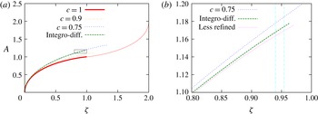
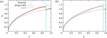
A graph of the solution (5.1) is plotted in figure 3. In the first instance we focus on solutions with
 $0\leqslant \unicode[STIX]{x1D701}\leqslant 1$
and
 $0\leqslant A\leqslant 1$
which is what (5.1) describes (although figure 3 includes a solution branch defined all the way up to
 $\unicode[STIX]{x1D701}=2$
and
 $A=2$
, as we will discuss shortly).
(a) Graph of
 $A$
versus
 $\unicode[STIX]{x1D701}$
(a rescaled version of angle through which the front turns
 $\unicode[STIX]{x1D6FC}$
versus distance from the top boundary
 $1-y$
) applicable to the upper region of the solution domain. The curve labelled
 $c=1$
is based on assuming that
 $\text{d}s/\text{d}y$
(with
 $s$
being path length travelled) is the same (at leading order) as
 $\text{d}x/\text{d}y$
and corresponds to (5.1). Although the
 $c=1$
case does admit a branch of solutions with
 $A>1$
(equivalent to saying that
 $\unicode[STIX]{x1D6FC}$
can overshoot the value predicted by the Velde solution lower down in the solution domain) the
 $A$
versus
 $\unicode[STIX]{x1D701}$
curve plotted here exhibits an inflection at
 $A=1$
(which is not observed in simulation data (Torres-Ulloa Reference Torres-Ulloa2015)). Alternate solutions assuming
 $\text{d}s/\text{d}y$
is less than
 $\text{d}x/\text{d}y$
are also given, parameterised by a value
 $c$
(the ratio between
 $\text{d}s/\text{d}y$
and
 $\text{d}x/\text{d}y$
being equal to
 $2c-1$
): these solutions are given by (6.2). The case
 $c=0.9$
is plotted (and is close to the original
 $c=1$
data set). The case of main interest is however
 $c=0.75$
. Data obtained from an integro-differential equation system (7.19) and (7.21) are also shown and are very close to the
 $c=0.75$
data set. (b) A zoomed view comparing the
 $c=0.75$
data set with the numerical solution of the integro-differential equation which is discretised into 1000 intervals. The curve labelled ‘less refined’ is for the integro-differential equation discretised into only 100 intervals. A discretisation into 10 000 intervals (albeit not plotted here) is indistinguishable on the scale of the graph from that for 1000 intervals. The vertical lines indicate the
 $\unicode[STIX]{x1D701}$
values at which the solutions generated are found to match onto the lower region of the solution domain
 $\unicode[STIX]{x1D701}\approx 0.94$
(for the
 $c=0.75$
solution) and
 $\unicode[STIX]{x1D701}\approx 0.954$
(for the integro-differential equation).

Note that for small
 $A\ll 1$
, the right-hand side of (5.1) Taylor expands to
 $A^{2}/2$
and hence for
 $\unicode[STIX]{x1D701}\ll 1$
, it follows
 $A\sim \sqrt{2\unicode[STIX]{x1D701}}$
. In that case,
 $\unicode[STIX]{x1D6FC}\equiv \sqrt{t/2}A$
becomes approximately
 $\sqrt{t\unicode[STIX]{x1D701}}\equiv \sqrt{2(1-y)}$
. This is the same behaviour (i.e. a mild singularity) near the top boundary as has been found for the late-time asymptotic solution (Grassia et al.
Reference Grassia, Mas-Hernández, Shokri, Cox, Mishuris and Rossen2014) (and is applicable here because the material points in question have spent the overwhelming majority of their history on the top boundary, only having left the top boundary comparatively recently). It is interesting to note that this finding justifies the numerical procedure proposed by Grassia et al. (Reference Grassia, Mas-Hernández, Shokri, Cox, Mishuris and Rossen2014) for placement of material points that were newly introduced near the top boundary which assumed a mild singularity was present. Formally Grassia et al. (Reference Grassia, Mas-Hernández, Shokri, Cox, Mishuris and Rossen2014) only proved the validity of this procedure in the long-time limit
 $t\gg 1$
, but it evidently has broader applicability. Moreover this same behaviour near the top boundary can actually also be obtained from (4.18) as both (4.17) and (4.18) reduce to
 $A_{\unicode[STIX]{x1D701}}\approx 1/A$
in this limit (with in addition
 $A\gg \unicode[STIX]{x1D701}$
in this same limit). This predicted behaviour immediately adjacent to the top boundary does not then require an assumption that
 $\text{d}s/\text{d}y\approx \text{d}x/\text{d}y$
since (4.18) does not make that assumption.
Moving away from the top boundary, equation (5.1) given above rearranges to
 $$\begin{eqnarray}1-\unicode[STIX]{x1D701}=(1-A)(1+\log (1/(1-A))).\end{eqnarray}$$
When
 $\unicode[STIX]{x1D701}$
and
 $A$
are both close to unity (which we expect to happen moving downwards through the upper region towards the lower region), we have an approximation
 $$\begin{eqnarray}1-\unicode[STIX]{x1D701}\approx (1-A)\log (1/(1-A))\end{eqnarray}$$
and hence
 $$\begin{eqnarray}\log (1-\unicode[STIX]{x1D701})\approx \log (1-A)+\log \log (1/(1-A)).\end{eqnarray}$$
To a very crude approximation it follows from (5.4) that
 $\log (1-A)\sim \log (1-\unicode[STIX]{x1D701})$
and hence substituting this result into (5.2)
 $$\begin{eqnarray}1-A\approx (1-\unicode[STIX]{x1D701})(1+\log (1/(1-\unicode[STIX]{x1D701})))^{-1}.\end{eqnarray}$$
The implication is that, in the limit as
 $\unicode[STIX]{x1D701}\rightarrow 1$
and
 $A\rightarrow 1$
,
 $A$
varies more slowly than
 $\unicode[STIX]{x1D701}$
, i.e. rescaled front orientation angle varies more slowly than rescaled distance. If indeed the matching point between the upper and lower regions occurs at
 $\unicode[STIX]{x1D701}=A=1$
, this is consistent with the curvature of the front being small near the matching point. We have already commented (see § 2.5) that numerical schemes for simulating pressure-driven growth become particularly difficult to implement when curvature is low, as even small perturbations can then convert convex shapes into a potentially problematic concave ones: it is unsurprising therefore that previous work (Grassia et al.
Reference Grassia, Mas-Hernández, Shokri, Cox, Mishuris and Rossen2014) has encountered numerical challenges here.
Interestingly (4.17) for the upper region of the foam front actually admits solutions for
 $\unicode[STIX]{x1D701}$
and
 $A$
both greater that unity: if one replaces
 $\unicode[STIX]{x1D701}$
by
 $2-\unicode[STIX]{x1D701}$
and
 $A$
by
 $2-A$
within (5.1) then a different solution branch is obtained. This branch is also plotted on figure 3 covering the domain
 $1\leqslant \unicode[STIX]{x1D701}\leqslant 2$
and
 $1\leqslant A\leqslant 2$
. The existence of this solution branch raises the possibility that the value of
 $A$
, even within the upper region, might rise above unity, in which case in order to match onto the top of the lower region (which has
 $A=1$
) a concave corner would be required. We will see later on (§ 6) that concave corners can and do indeed occur, albeit not in the fashion that (4.17) predicts. For the present however we continue to explore the consequences of assuming that the upper and lower regions join up without a concave corner.
5.2 Re-expressing solution in terms of injection time
It is possible to re-express the solution (5.1) above in terms of an ‘injection time’, defined as a time at which material points were injected from the top boundary onto the foam front, a concept that has already been described by Grassia et al. (Reference Grassia, Mas-Hernández, Shokri, Cox, Mishuris and Rossen2014).
The injection time
 $t_{inj}$
can take any value between zero and the current time
 $t$
. If
 $t_{inj}\rightarrow t$
then material points are extremely close to the top boundary (i.e.
 $\unicode[STIX]{x1D701}\ll 1$
and hence
 $A\ll 1$
). On the other hand if
 $t_{inj}\ll t$
then material points are close to the matching point at which material which has been injected (constituting the upper region) joins up with material which has been continuously on the front since time zero (constituting the lower region). In that case we anticipate
 $\unicode[STIX]{x1D701}\approx 1$
and also (at least according to (5.1))
 $A\approx 1$
.
It turns out that the solution (5.1) given above follows from a particularly simple functional form
 $$\begin{eqnarray}\unicode[STIX]{x1D6FC}=(t-t_{inj})/\sqrt{2t}.\end{eqnarray}$$
This equation is ‘exact’ in the same sense that (5.1) is, i.e. it manages to solve (4.17) exactly, notwithstanding the fact that (4.17) is itself a small-time approximation. Here we proceed by assuming that
 $\unicode[STIX]{x1D6FC}$
follows (5.6) and then demonstrating that (5.1) follows as a consequence. If (5.6) holds, then (using the definition
 $\unicode[STIX]{x1D6FC}\equiv \sqrt{t/2}A$
)
 $$\begin{eqnarray}A=1-t_{inj}/t,\end{eqnarray}$$
a very simple relation indicating that the higher the fraction of total time a material point has spent on the front since being injected, the more the material element upon which it finds itself has reoriented. On the other hand, if (5.6) holds, then we can solve (4.6) for
 $y$
versus
 $t$
. The solution is
 $$\begin{eqnarray}y=1-t/2+t_{inj}/2+(1/2)t_{inj}\log (t/t_{inj}).\end{eqnarray}$$
Since
 $\unicode[STIX]{x1D701}\equiv (1-y)/(t/2)$
, it follows
 $$\begin{eqnarray}\unicode[STIX]{x1D701}=1-\frac{t_{inj}}{t}+\frac{t_{inj}}{t}\log \frac{t}{t_{inj}}.\end{eqnarray}$$
Substituting from (5.7) then gives (5.1).
Note that differentiating
 $A$
and
 $\unicode[STIX]{x1D701}$
(or equivalently
 $\unicode[STIX]{x1D6FC}$
and
 $y$
) with respect to
 $t_{inj}$
at constant
 $t$
, corresponds to moving from material point to material point for a given instantaneous curve shape. Notice that
 $$\begin{eqnarray}-\frac{\unicode[STIX]{x2202}\unicode[STIX]{x1D6FC}}{\unicode[STIX]{x2202}y}=-\frac{\unicode[STIX]{x2202}\unicode[STIX]{x1D6FC}/\unicode[STIX]{x2202}t_{inj}}{\unicode[STIX]{x2202}y/\unicode[STIX]{x2202}t_{inj}}=\frac{1/\sqrt{2t}}{(1/2)\log (t/t_{inj})},\end{eqnarray}$$
where the denominator diverges (albeit exceedingly slowly) as
 $t_{inj}\rightarrow 0$
. This is actually a demonstration that the predicted curvature falls to zero near the expected matching point, since (recalling that
 ${\mathcal{S}}$
is distance measured along the front in a downwards direction) the curvature becomes
 $\unicode[STIX]{x2202}\unicode[STIX]{x1D6FC}/\unicode[STIX]{x2202}{\mathcal{S}}$
which is equivalent to
 $-\unicode[STIX]{x2202}\unicode[STIX]{x1D6FC}/\unicode[STIX]{x2202}y$
for a front that is nearly vertical, such as would happen when
 $t\ll 1$
.
This situation near the matching point with
 $t_{inj}\ll t$
contrasts with what is happening at the top boundary where
 $t_{inj}\rightarrow t$
. Near the top
 $\unicode[STIX]{x1D6FC}\sim \sqrt{2(1-y)}$
as we saw in § 5.1 and hence
 $-\unicode[STIX]{x2202}\unicode[STIX]{x1D6FC}/\unicode[STIX]{x2202}y\sim 1/\sqrt{2(1-y)}$
, so curvature is infinite at the top boundary.
5.3 Horizontal mismatch of front shape
One elegant feature of the solution (5.1) for the upper region of the foam front is that at
 $y=1-t/2$
(equivalently at
 $\unicode[STIX]{x1D701}=1$
) it has
 $A=1$
(equivalently
 $\unicode[STIX]{x1D6FC}=\sqrt{t/2}$
) which is the same
 $\unicode[STIX]{x1D6FC}$
value as would be predicted by the Velde solution for the lower region of the front as discussed in § 3 (see e.g. (3.5) assuming
 $t\ll 1$
and hence with
 $y=1-t/2$
at the top of the lower region being close to unity). Thus we have two solutions for the distinct regions of the front which have the same orientation at the same vertical location, suggesting that the solutions for the upper and lower regions might join up with the same orientation angle, as we have assumed to date. Unfortunately however it turns out that there is a horizontal mismatch between these solutions. The detailed explanation is given below, but some readers may prefer to skip directly to view the horizontal mismatch plotted in figure 4.
(a) Graph of
 $-\unicode[STIX]{x1D701}$
versus
 $-\unicode[STIX]{x1D6EF}$
(a rescaled version of
 $y$
versus
 $x$
) for the foam front. Solutions in the upper region of the domain are generated in the first instance assuming
 $\text{d}s/\text{d}y\approx \text{d}x/\text{d}y$
(curve labelled
 $c=1$
; with angle
 $A$
obtained from (5.1), and
 $\unicode[STIX]{x1D6EF}$
obtained from integrating
 $A$
via (5.16)) and subsequently with
 $\text{d}s/\text{d}y<\text{d}x/\text{d}y$
(curve labelled
 $c=0.75$
;
 $A$
obtained from (6.2)) and also shown is a curve where solutions were obtained via an integro-differential equation (7.19). These solutions for the upper region are required to intersect solutions that apply in the lower part of the domain (curve labelled lower region, given by (5.15)). For
 $c=1$
, no intersection is seen (at least not in the neighbourhood of
 $\unicode[STIX]{x1D701}=1$
). (b) In this zoomed view, intersections are seen in the case
 $c=0.75$
and in the case of the integro-differential equation, respectively for
 $\unicode[STIX]{x1D701}\approx 0.94$
and
 $\unicode[STIX]{x1D701}\approx 0.954$
(horizontal lines).

We know via (3.13) that in the lower region of the domain, to a good approximation
 $x\approx \sqrt{2yt+t^{2}/6}$
which can be obtained via a perturbation expansion that improves upon the original Velde solution (3.2). We know moreover that the leading edge at the top of the front is at location
 $x=\sqrt{2t}$
with
 $y=1$
. Moving away from
 $y=1$
, if we define
 $\unicode[STIX]{x1D709}$
to be the horizontal distance behind the leading edge (
 $\unicode[STIX]{x1D709}\equiv \sqrt{2t}-x$
), it follows via a difference of squares (remembering that
 $x$
is itself close to
 $\sqrt{2t}$
)
 $$\begin{eqnarray}\unicode[STIX]{x1D709}\approx \frac{(\sqrt{2t}-x)(\sqrt{2t}+x)}{2\sqrt{2t}}\approx \frac{(2t-x^{2})}{2\sqrt{2t}}\approx \frac{2t-2yt-t^{2}/6}{2\sqrt{2t}}.\end{eqnarray}$$
If we put
 $y=1-t/2$
(the expected matching point), we deduce
 $\unicode[STIX]{x1D709}\approx 5t^{3/2}/(12\sqrt{2})$
via this ‘improved’ Velde solution (3.13).
There is however an alternative way of computing
 $\unicode[STIX]{x1D709}$
, as a function of
 $y$
, namely integrating
 $\text{d}x/\text{d}y$
to measure a change in
 $x$
for a given change in
 $y$
. For
 $t\ll 1$
, we can approximate
 $\text{d}x/\text{d}y$
by the angle
 $\unicode[STIX]{x1D6FC}$
, and therefore
 $$\begin{eqnarray}\unicode[STIX]{x1D709}\approx \int _{y}^{1}\unicode[STIX]{x1D6FC}\,\text{d}y\end{eqnarray}$$
and hence at
 $y=1-t/2$
,
 $$\begin{eqnarray}\unicode[STIX]{x1D709}|_{y=1-t/2}\approx \int _{1-t/2}^{1}\unicode[STIX]{x1D6FC}\,\text{d}y,\end{eqnarray}$$
where
 $\unicode[STIX]{x1D6FC}$
is based on the shape of the upper region. Using (5.8) to change the integration variable from
 $y$
to
 $t_{inj}$
, this can also be written
 $$\begin{eqnarray}\unicode[STIX]{x1D709}|_{y=1-t/2}\approx \int _{0}^{t}\unicode[STIX]{x1D6FC}\frac{\unicode[STIX]{x2202}y}{\unicode[STIX]{x2202}t_{inj}}\,\text{d}t_{inj}=\int _{0}^{t}\frac{(t-t_{inj})}{\sqrt{2t}}\frac{1}{2}\log \frac{t}{t_{inj}}\,\text{d}t_{inj}=3t^{3/2}/(8\sqrt{2}),\end{eqnarray}$$
where (5.6) has also been used in addition to (5.8). This
 $\unicode[STIX]{x1D709}$
value in (5.14) is smaller than the result obtained earlier by a factor
 $3/8\times 12/5=9/10$
.
In other words, moving downwards from the top boundary, the solution
 $\unicode[STIX]{x1D6FC}$
versus
 $y$
predicted by (5.1) does not curve sufficiently as to join up with the
 $x$
versus
 $y$
function in the lower region. The predicted horizontal location of the bottom of the upper region (5.14) is not the same as that of the top of the lower region ((5.11) with
 $y=1-t/2$
). We can see this graphically in figure 4. In this figure we have defined a variable
 $\unicode[STIX]{x1D6EF}=(\sqrt{2t}-x)/t^{3/2}\equiv \unicode[STIX]{x1D709}/t^{3/2}$
along with
 $\unicode[STIX]{x1D701}=(1-y)/(t/2)$
, and have plotted
 $-\unicode[STIX]{x1D701}$
against
 $-\unicode[STIX]{x1D6EF}$
, which has the same orientation as a graph of
 $y$
versus
 $x$
.
In terms of
 $\unicode[STIX]{x1D6EF}$
, equation (5.11) describing the lower region of the front in the neighbourhood of the matching point becomes
 $$\begin{eqnarray}\unicode[STIX]{x1D6EF}\approx \frac{\unicode[STIX]{x1D701}}{2\sqrt{2}}-\frac{1}{12\sqrt{2}}\end{eqnarray}$$
whilst in the upper region we have (via (5.12))
 $$\begin{eqnarray}\unicode[STIX]{x1D6EF}\approx \frac{1}{2\sqrt{2}}\int _{0}^{\unicode[STIX]{x1D701}}A\,\text{d}\unicode[STIX]{x1D701},\end{eqnarray}$$
where
 $A$
is obtained in the first instance from (5.1).
Clearly in figure 4 there is no intersection between the upper and lower region curves near
 $\unicode[STIX]{x1D701}=1$
, at least when (5.1) is used to describe the upper region. In order to make the curves intersect, what we require in the upper region is a solution for
 $\unicode[STIX]{x1D6FC}$
versus
 $y$
that curves slightly more than that computed above, giving a slightly larger
 $\unicode[STIX]{x1D6FC}$
at any given
 $y$
(or equivalently a slightly larger
 $A$
at any given
 $\unicode[STIX]{x1D701}$
). As was mentioned in § 4.3.1, the solution to (4.18), in lieu of (4.17) which is what we have been solving to date, should have that property.
5.4 Predicted difference between
 $\text{d}s/\text{d}y$
and
$\text{d}x/\text{d}y$


In addition to the horizontal mismatch discussed above, it is possible to demonstrate that (5.1) contradicts the assumptions used to derive it. It turns out to predict that
 $\text{d}s/\text{d}y$
(with
 $s$
being a history-dependent path length variable) is significantly less than
 $\text{d}x/\text{d}y$
, even though (4.17) (of which (5.1) is the solution) was derived assuming
 $\text{d}s/\text{d}y\approx \text{d}x/\text{d}y$
. Some readers may wish to turn directly to (5.25)–(5.26) which demonstrate that this assumption is invalid. Nonetheless we will see that (5.1) still manages to make useful predictions at least on parts of the front, because there are parts of the front for which the local shape is unaffected in spite of the aforementioned contradiction.
The analysis proceeds as follows. To a good approximation
 $$\begin{eqnarray}s\approx \int _{0}^{x}\left(1+\frac{1}{2}\frac{({\dot{y}})^{2}}{({\dot{x}})^{2}}\right)\,\text{d}x\approx \int _{0}^{x}\left(1+\frac{1}{2}\unicode[STIX]{x1D6FC}^{2}\right)\,\text{d}x,\end{eqnarray}$$
where we have used the fact that at early time vertical velocity is much weaker than horizontal velocity
 $|{\dot{y}}|\ll |{\dot{x}}|$
, and also at leading order near the top boundary,
 ${\dot{y}}\approx -\unicode[STIX]{x1D6FC}/s$
and
 ${\dot{x}}\approx 1/s$
via e.g. (3.6) and (3.1).
Evaluating the integral in (5.17) is not possible without a priori information about
 $\unicode[STIX]{x1D6FC}$
.
We know however via (5.6) that a material point injected onto the front at time
 $t_{inj}$
has an
 $\unicode[STIX]{x1D6FC}$
value
 $\unicode[STIX]{x1D6FC}=(t-t_{inj})/\sqrt{2t}$
. Substituting this into (5.17) we deduce
 $$\begin{eqnarray}s\approx x+\int _{t_{inj}}^{t}\frac{(t-t_{inj})^{2}}{4t}\,\frac{\text{d}t}{\sqrt{2t}}=x+\frac{(t-t_{inj})^{3}}{12\sqrt{2}t^{3/2}},\end{eqnarray}$$
where we have used the fact that
 $\text{d}x={\dot{x}}\,\text{d}t\approx \text{d}t/s\approx \text{d}t/\sqrt{2t}$
.
We know moreover that
 $$\begin{eqnarray}x=\sqrt{2t}-\unicode[STIX]{x1D709}\approx \sqrt{2t}-\int _{y}^{1}\unicode[STIX]{x1D6FC}\,\text{d}y.\end{eqnarray}$$
Changing the integration variable from
 $y$
to
 $t_{inj}$
using (5.8) which implies
 $\unicode[STIX]{x2202}y/\unicode[STIX]{x2202}t_{inj}=(1/2)\log (t/t_{inj})$
, we deduce
 $$\begin{eqnarray}x\approx \sqrt{2t}-\int _{t_{inj}}^{t}\frac{(t-t_{inj})}{\sqrt{2t}}\frac{1}{2}\log (t/t_{inj})\,\text{d}t_{inj}\end{eqnarray}$$
and hence
 $$\begin{eqnarray}x\approx \sqrt{2t}-\frac{t^{3/2}}{2\sqrt{2}}\left(-\frac{t_{inj}}{t}\left(1-\frac{t_{inj}}{2t}\right)\log (t/t_{inj})-\frac{t_{inj}}{t}\left(1-\frac{t_{inj}}{4t}\right)+\frac{3}{4}\right).\end{eqnarray}$$
Combining (5.18) and (5.21) we deduce
 $$\begin{eqnarray}s\approx \sqrt{2t}-\frac{t^{3/2}}{2\sqrt{2}}\left(-\frac{t_{inj}}{t}\left(1-\frac{t_{inj}}{2t}\right)\log (t/t_{inj})-\frac{t_{inj}}{t}\left(1-\frac{t_{inj}}{4t}\right)+\frac{3}{4}\right)+\frac{t^{3/2}}{12\sqrt{2}}(1-t_{inj}/t)^{3}.\end{eqnarray}$$
The physical content of both (5.21) and (5.22) is that as
 $t_{inj}$
falls below
 $t$
(corresponding to choosing material points further and further below the top boundary) both
 $x$
and
 $s$
fall short of the value
 $\sqrt{2t}$
(which is the displacement of the front on the top boundary), however they fall short of
 $\sqrt{2t}$
by differing amounts. The predicted ratio between the
 $s$
-shortfall and the
 $x$
-shortfall is sensitive to
 $t_{inj}/t$
(and hence is sensitive to the precise location within the upper region of the front which depends on
 $t_{inj}/t$
). In what follows the limiting case
 $t_{inj}\rightarrow t$
(i.e. the behaviour at the very top of the upper region) is considered.
5.4.1 Limiting case
$t_{inj}\rightarrow t$

A Taylor expansion of (5.21) for
 $t_{inj}$
close to
 $t$
(or in other words for vertical locations exceedingly close to the top boundary) reveals
 $$\begin{eqnarray}x\approx \sqrt{2t}-\frac{t^{3/2}}{6\sqrt{2}}(1-t_{inj}/t)^{3}\end{eqnarray}$$
from which it then follows
 $$\begin{eqnarray}s\approx \sqrt{2t}-\frac{t^{3/2}}{12\sqrt{2}}(1-t_{inj}/t)^{3},\end{eqnarray}$$
which can also be expressed in the form (using results from Grassia et al. (Reference Grassia, Mas-Hernández, Shokri, Cox, Mishuris and Rossen2014))
 $$\begin{eqnarray}\displaystyle & \displaystyle x\approx \sqrt{2t}-\frac{2\sqrt{2}}{3}(1-y)^{3/2} & \displaystyle\end{eqnarray}$$
 $$\begin{eqnarray}\displaystyle & \displaystyle s\approx \sqrt{2t}-\frac{\sqrt{2}}{3}(1-y)^{3/2}. & \displaystyle\end{eqnarray}$$
Hence very close to the top boundary of the front at least, the variation of
 $s$
with respect to position is exactly half the variation of
 $x$
with respect to position, i.e.
 $\text{d}s/\text{d}y$
is half of
 $\text{d}x/\text{d}y$
.
Some comments are pertinent. The predictions of (5.21) and (5.22) for the extent that
 $x$
and
 $s$
vary potentially contain errors/artefacts as those equations were derived based on an approximate front shape that assumed equality between
 $\text{d}x/\text{d}y$
and
 $\text{d}s/\text{d}y$
, but subsequently discovered that assumption is contradicted. Equations (5.23)–(5.24) or equivalently (5.25)–(5.26), although they only apply to
 $t_{inj}$
values very close to
 $t$
, and need not apply all the way to the matching point for which
 $t_{inj}\ll t$
, do not suffer from such artefacts. In the present limit
 $t_{inj}/t\rightarrow 1$
(which also implies
 $(1-y)\ll t/2$
and hence similarity variable
 $\unicode[STIX]{x1D701}\equiv (1-y)/(t/2)\ll 1$
), we obtain the same results regardless of whether we use (4.4) or (4.5) to obtain
 $\dot{\unicode[STIX]{x1D6FC}}$
, or equivalently regardless of whether we use (4.17) or (4.18) to obtain
 $A_{\unicode[STIX]{x1D701}}$
. In the neighbourhood of the top of the front, the numerators of both (4.17) and (4.18) involve subtracting an exceedingly small term from unity, implying insensitivity to what the exact value of that exceedingly small term is. Hence the difference that is predicted between
 $\text{d}x/\text{d}y$
and
 $\text{d}s/\text{d}y$
neighbouring the top of the front is not merely an artefact of using (4.17) instead of (4.18). This then gives a strong indication that it might be possible for
 $\text{d}s/\text{d}y$
to remain smaller than
 $\text{d}x/\text{d}y$
throughout the entire upper region of the front, all the way down to the matching point, in which case (4.18) predicts a different
 $A$
versus
 $\unicode[STIX]{x1D701}$
relation from that given in (5.1) which relied upon (4.17). This alternative
 $A$
versus
 $\unicode[STIX]{x1D701}$
relation for the upper region should join up with the solution in the lower region without exhibiting the horizontal mismatch that was observed previously (in § 5.3) although the cost of eliminating the horizontal mismatch, could be that the front orientation angles might cease to be aligned where the upper and lower regions meet (i.e. a concave corner might be present). In the following section, we present a technique for determining the alternative
 $A$
versus
 $\unicode[STIX]{x1D701}$
relation.
6 Alternative solution for upper region
$A$
versus
$\unicode[STIX]{x1D701}$


In what follows we make an assumption that
 $\text{d}s/\text{d}y$
remains half of
 $\text{d}x/\text{d}y$
all the way down to the matching point (rather than merely exceedingly close to the top boundary as has been demonstrated in § 5.4.1). There is no a priori reason why this should be the case, but as we will see when we compare with more accurate solutions later on, the assumption actually turns out to be a remarkably good one.
If we substitute
 $\text{d}s/\text{d}y=(\text{d}x/\text{d}y)/2$
into (4.18), then in lieu of (4.17), we now have
 $$\begin{eqnarray}A_{\unicode[STIX]{x1D701}}\approx (1-cA)/(A-\unicode[STIX]{x1D701}),\end{eqnarray}$$
where specifically
 $c=3/4$
, with the ratio between
 $\text{d}s/\text{d}y$
and
 $\text{d}x/\text{d}y$
being
 $2c-1$
.
Equation (6.1) but with
 $c$
taken to be a free parameter (somewhere between
 $3/4$
and unity, in the latter case (4.17) being recovered) is actually quite a powerful equation which can help us to understand how the
 $A$
versus
 $\unicode[STIX]{x1D701}$
relation can be varied to ensure that the upper and lower regions of the front can be made to intersect. The solution of (6.1) is
 $$\begin{eqnarray}\unicode[STIX]{x1D701}=1/c-(1-cA)/(c(1-c))+(1-cA)^{1/c}/(1-c),\end{eqnarray}$$
where in keeping with the practice adopted in § 5.1 we use an equal sign in (6.2) rather than an approximation sign, reflecting the fact that this is an exact solution of (6.1), albeit equation (6.1) is itself a small-time asymptotic approximation to the true governing equation of the front. With (6.2), it is now quite possible for
 $A$
to exceed unity even for
 $\unicode[STIX]{x1D701}<1$
. In fact
 $A$
attains the value unity when
 $\unicode[STIX]{x1D701}=(1-c)^{-1+1/c}$
. Moreover
 $A$
attains the value
 $1/c$
when
 $\unicode[STIX]{x1D701}=1/c$
.
The function (6.2) is plotted on figure 3, and, as
 $c$
decreases,
 $A$
values are clearly seen to be larger than those predicted by (5.1). According to (5.16),
 $\unicode[STIX]{x1D6EF}$
values are also larger at any given
 $\unicode[STIX]{x1D701}$
, implying in figure 4 that the upper region of the front curves more than previously, such that the horizontal location of any point on the upper region of the front is further back from the leading edge than previously. This then gives an opportunity for the upper and lower regions of the front to intersect without any horizontal mismatch. In what follows we identify this intersection point (§ 6.1), and then relate its location to injection times (§ 6.2), and also to the distances that material points have travelled (§ 6.3).
6.1 Matching or ‘cross-over’ point
Assuming that (6.1) with
 $c=3/4$
is a good representation of the shape of the front over the entire upper region of the domain, it is possible to identify a matching or ‘cross-over’ point at which the front shapes computed in the upper and lower region of the domain intersect or ‘cross-over’ one another. The cross-over point (still assuming
 $c=3/4$
) is found to be around
 $\unicode[STIX]{x1D701}_{cross}\approx 0.94$
, corresponding to an
 $A$
value
 $A_{cross}\approx 1.18$
: these values can be easily read off from figures 3(b) and 4(b) respectively.
The fact that
 $A_{cross}$
exceeds unity is encouraging: it suggests that the orientation angle of the upper region of the front overshoots that on the lower region, so the front has a concave corner there. The value of
 $A$
jumps from
 $A_{cross}\approx 1.18$
immediately above the concavity to unity immediately below it, or in other words, the front orientation angle
 $\unicode[STIX]{x1D6FC}$
, which is related to
 $A$
via
 $\unicode[STIX]{x1D6FC}\equiv \sqrt{t/2}A$
, jumps from around
 $0.834\sqrt{t}$
to around
 $0.707\sqrt{t}$
, implying a jump of 0.09 radians or approximately
 $5^{\circ }$
at the instant
 $t=0.5$
(which happens to be the specific time at which the distance through which the top of the front has advanced, namely
 $\sqrt{2t}$
, is the same as the front’s depth, i.e. unity).
The prediction that
 $\unicode[STIX]{x1D701}_{cross}$
is smaller than unity is slightly curious: it implies that the depth
 $1-y$
below the top boundary at which the concave corner is located is slightly less than the depth
 $t/2$
to which the material point initially at the top of the lower region of the front is expected to migrate. This in turn suggests that, rather than the concave corner consuming material points on the front on either side of it (as we expect in conventional pressure-driven growth (Grassia et al.
Reference Grassia, Mas-Hernández, Shokri, Cox, Mishuris and Rossen2014)), material points are actually being extracted from the concavity on the side below the concave corner (a behaviour which has only previously been observed in pressure-driven growth systems for which the reservoir properties are taken to be highly anisotropic (Grassia et al.
Reference Grassia, Torres-Ulloa, Berres, Mas-Hernández and Shokri2016), and not in isotropic systems as are considered here). Indeed recognising that the location
 $\unicode[STIX]{x1D701}=1$
on the lower part of the curve (which is already a small but finite distance below the concavity) corresponds to a material point which was initially adjacent to the top surface, any points between
 $\unicode[STIX]{x1D701}=\unicode[STIX]{x1D701}_{cross}$
and
 $\unicode[STIX]{x1D701}=1$
must have been extracted from the corner itself.
The reason the points at the top of the lower region of the front manage to ‘outrun’ those at the bottom of the upper region (despite the fact that points on the upper region immediately adjacent to the corner are instantaneously moving downward faster owing to their greater
 $A$
value remembering that
 ${\dot{y}}\approx -A/2$
via (4.10)) is that the upper region of the curve exhibits strong spatio-temporal non-uniformities in the vertical velocity component. Thus knowing the instantaneous vertical velocity alone (which is
 $-A_{cross}/2$
immediately above the corner) is inadequate for determining the vertical distance that points in the upper region have propagated over a given time interval up to time
 $t$
, even in the case of arbitrarily small values of
 $t$
. A conventional pressure-driven growth picture of a concavity that consumes material points on both sides of it (Grassia et al.
Reference Grassia, Mas-Hernández, Shokri, Cox, Mishuris and Rossen2014), would apply to a system for which velocities of neighbouring material points are locally nearly uniform and nearly constant in time, but that is not the case here.
To reiterate, the material point which is instantaneously at location
 $\unicode[STIX]{x1D701}_{cross}$
at time
 $t$
cannot have spent its entire history at or near that particular
 $\unicode[STIX]{x1D701}$
value. This follows because points at location
 $\unicode[STIX]{x1D701}_{cross}$
have an instantaneous vertical velocity
 ${\dot{y}}$
equal to
 $-A_{cross}/2$
. Were the point to move with that velocity at all times between zero and
 $t$
, it would attain a
 $y$
value
 $y=1-A_{cross}t/2$
and hence a
 $\unicode[STIX]{x1D701}$
value of
 $\unicode[STIX]{x1D701}=A_{cross}$
instead of its actual location
 $\unicode[STIX]{x1D701}=\unicode[STIX]{x1D701}_{cross}$
. Spatio-temporal non-uniformity in the vertical trajectories of material points is an essential feature of the upper region.
6.2 Minimum permitted injection time
As was mentioned above, at any given time
 $t$
, the material point in the upper region of the solution domain immediately adjacent to the concave corner
 $\unicode[STIX]{x1D701}=\unicode[STIX]{x1D701}_{cross}$
, cannot have always been at that location, but instead must have migrated there from smaller
 $\unicode[STIX]{x1D701}$
values (which must also have a lesser downward velocity component) earlier on. Points in the upper region of the front continue to be consumed by the concave corner, so there must exist a well defined injection time
 $t_{inj}$
(itself dependent on the current time
 $t$
) at which the point instantaneously at the concave corner was injected onto the front from the top boundary. This is the minimum permitted injection time (in the sense that, at time
 $t$
, out of all the currently surviving points on the upper region of the front, the point that is currently adjacent to the concave corner was injected earlier than any of the others): we denote this minimum permitted injection time
 $t_{inj(min)}$
. Any material points which were injected onto the front earlier than time
 $t_{inj(min)}$
have already been consumed by the concave corner. Consequently, whereas points in the lower region of the solution domain have been moving downward over the entire interval of time from zero to
 $t$
, those in the upper region have only been moving downward for an interval no longer than
 $t-t_{inj(min)}$
(with
 $t_{inj(min)}$
depending on
 $t$
).
We expect the following relations (which serve to fix the value of
 $t_{inj(min)}$
) to be valid
 $$\begin{eqnarray}\int _{t_{inj(min)}}^{t}\frac{A}{2}\,\text{d}t^{\prime }=\unicode[STIX]{x1D701}_{cross}\frac{t}{2},\end{eqnarray}$$
(which uses the fact that the downward velocity component
 ${\dot{y}}$
of material points is
 $A/2$
, with
 $\unicode[STIX]{x1D701}=\unicode[STIX]{x1D701}_{cross}$
being a distance
 $1-y=\unicode[STIX]{x1D701}_{cross}t/2$
below the top boundary) and also
 $$\begin{eqnarray}\int _{t_{inj(min)}}^{t}\frac{(A-\unicode[STIX]{x1D701})}{t^{\prime }}\,\text{d}t^{\prime }=\unicode[STIX]{x1D701}_{cross}\end{eqnarray}$$
(using the expression (4.11) for
 $\dot{\unicode[STIX]{x1D701}}$
of a material point). Nonetheless
 $t_{inj(min)}$
(or more precisely the ratio between
 $t_{inj(min)}$
and
 $t$
) can be obtained most straightforwardly by manipulating the expression (4.11) for
 $\dot{\unicode[STIX]{x1D701}}$
as follows
 $$\begin{eqnarray}\text{d}\log t/\text{d}\unicode[STIX]{x1D701}=1/(A-\unicode[STIX]{x1D701})\end{eqnarray}$$
and hence (integrating from
 $t_{inj(min)}$
to
 $t$
, or equivalently from 0 to
 $\unicode[STIX]{x1D701}_{cross}$
)
 $$\begin{eqnarray}\log (t/t_{inj(min)})=\int _{0}^{\unicode[STIX]{x1D701}_{cross}}\text{d}\unicode[STIX]{x1D701}/(A-\unicode[STIX]{x1D701}).\end{eqnarray}$$
If
 $A$
versus
 $\unicode[STIX]{x1D701}$
happened to be known numerically at any given time (e.g. from a numerical simulation technique such as that described later on in § 8) the above equation gives a way of determining
 $t_{inj(min)}/t$
at the matching point
 $\unicode[STIX]{x1D701}_{cross}$
without even making a priori assumptions about the existence of a similarity solution. Moreover to the extent that (6.1) applies
 $$\begin{eqnarray}\log (t/t_{inj(min)})=\int _{0}^{A_{cross}}\frac{\unicode[STIX]{x1D701}_{A}\,\text{d}A}{(A-\unicode[STIX]{x1D701})}=\int _{0}^{A_{cross}}\frac{\text{d}A}{(1-cA)}=\frac{1}{c}\log (1/(1-cA_{cross}))\end{eqnarray}$$
and hence
 $$\begin{eqnarray}t_{inj(min)}/t=(1-cA_{cross})^{1/c}.\end{eqnarray}$$
In other words, the ratio
 $t_{inj(min)}/t$
for the longest surviving point on the upper region of the front (i.e. the longest surviving point which has not yet been consumed by the lower region of the front), can be obtained solely in terms of the parameters
 $c$
and
 $A_{cross}$
(with
 $c$
being estimated as
 $3/4$
and
 $A_{cross}$
being estimated as the ratio of the
 $\unicode[STIX]{x1D6FC}$
values either side of the concave corner at which the upper and lower regions of the front join together). Taking the value
 $A_{cross}\approx 1.18$
quoted previously, still with
 $c=3/4$
, we estimate
 $t_{inj(min)}\approx 0.056t$
.
6.3 Distances that material points travel to the matching point
One of the issues we have not yet discussed concerning the concave corner at the matching point is that material points immediately adjacent to the corner on either side could potentially have followed different paths to reach their current position. Hence there could potentially be two adjacent points on the front which have different
 $s$
values, i.e.
 $s$
is not necessarily continuous at a concave corner.
Adjacent to a concave corner, the direction of motion of material points is certainly discontinuous, since motion is along the front normal, and the front normal undergoes a discrete change in direction. However any discontinuity in
 $s$
would also imply that the speed of material points (which is just
 $y/s$
according to (2.6)) is necessarily discontinuous there. Nonetheless significant discontinuities are unlikely to manifest themselves at early times, since motion is primarily horizontal at early times, so that
 $s$
at leading order is almost the same as
 $x$
, regardless of the path followed to arrive at any
 $(x,y)$
location.
Specifically the relationship giving
 $s$
for the point initially at the top of the lower region is (following § 3.3)
 $$\begin{eqnarray}s\approx \int _{0}^{x}\left(1+\frac{1}{2}\frac{({\dot{y}})^{2}}{({\dot{x}})^{2}}\right)\,\text{d}x=x+\int _{0}^{t}\frac{1}{2}\frac{1/4}{1/(2t^{\prime })}\,\frac{\text{d}t^{\prime }}{\sqrt{2t^{\prime }}}=x+(2t)^{3/2}/24\approx x(1+t/12),\end{eqnarray}$$
whereas that giving
 $s$
within the upper region is by analogy
 $$\begin{eqnarray}s\approx x+\int _{t_{inj}}^{t}\frac{1}{2}\frac{A^{2}/4}{1/(2t^{\prime })}\,\frac{\text{d}t^{\prime }}{\sqrt{2t^{\prime }}}=x+t_{inj}^{3/2}\int _{0}^{\unicode[STIX]{x1D713}}\frac{\sqrt{2}A^{2}}{8}\,\frac{\text{d}\unicode[STIX]{x1D713}^{\prime }}{(1-\unicode[STIX]{x1D713}^{\prime })^{5/2}},\end{eqnarray}$$
where we have defined a new variable
 $\unicode[STIX]{x1D713}$
to be
 $$\begin{eqnarray}\unicode[STIX]{x1D713}=1-t_{inj}/t,\end{eqnarray}$$
(with
 $\unicode[STIX]{x1D713}$
being the fraction of time relative to the current time
 $t$
that a given material point has been present on the front), and a corresponding dummy integration variable
 $\unicode[STIX]{x1D713}^{\prime }$
such that
 $\unicode[STIX]{x1D713}^{\prime }=1-t_{inj}/t^{\prime }$
, from which it follows
 $t^{\prime }=t_{inj}/(1-\unicode[STIX]{x1D713}^{\prime })$
and hence
 $\text{d}t^{\prime }=t_{inj}\,\text{d}\unicode[STIX]{x1D713}^{\prime }/(1-\unicode[STIX]{x1D713}^{\prime })^{2}$
. We can also consider
 $A$
to be a function of
 $\unicode[STIX]{x1D713}$
instead of being a function of either
 $\unicode[STIX]{x1D701}$
or
 $t_{inj}/t$
. The value of
 $\unicode[STIX]{x1D713}$
at the matching or cross-over point, which we denote
 $\unicode[STIX]{x1D713}_{cross}$
, is given by
 $\unicode[STIX]{x1D713}_{cross}=1-t_{inj(min)}/t$
. For the material point within the upper region immediately adjacent to the concave corner, the above (6.10) becomes
 $$\begin{eqnarray}\displaystyle s & {\approx} & \displaystyle x+\sqrt{2}t^{3/2}(1-\unicode[STIX]{x1D713}_{cross})^{3/2}\int _{0}^{\unicode[STIX]{x1D713}_{cross}}\frac{A^{2}}{8}\,\frac{\text{d}\unicode[STIX]{x1D713}^{\prime }}{(1-\unicode[STIX]{x1D713}^{\prime })^{5/2}}\nonumber\\ \displaystyle & {\approx} & \displaystyle x\left(1+t(1-\unicode[STIX]{x1D713}_{cross})^{3/2}\int _{0}^{\unicode[STIX]{x1D713}_{cross}}\frac{A^{2}}{8}\,\frac{\text{d}\unicode[STIX]{x1D713}^{\prime }}{(1-\unicode[STIX]{x1D713}^{\prime })^{5/2}}\right).\end{eqnarray}$$
Comparing (6.9) and (6.12), at any given time
 $t$
, and depending on the form of the function
 $A$
versus
 $\unicode[STIX]{x1D713}$
, it appears at first sight as though a discontinuity in the value of
 $s$
of up to order
 $t$
times
 $s$
itself could potentially occur.
Remember from § 6.1 however an unusual property for the concave corner: instead of consuming material points on both sides, immediately above the corner the system is consuming material points but immediately below the corner the system is creating them. As a result (6.9) gives the
 $s$
value for the material point within the lower region that was initially at the top of the front, but not the
 $s$
value of newly created points that lie between it and the concave corner. Indeed those newly created material points need to be assigned an
 $s$
value at the time they are created. If points created immediately below the corner are given the same
 $s$
value as those that are being destroyed immediately above the corner, then continuity of
 $s$
through the corner can be ensured. Interestingly a recent simulation study (Torres-Ulloa Reference Torres-Ulloa2015) on pressure-driven growth using a completely different numerical simulation technique (i.e. an Eulerian technique which does not make reference to material points) did indeed indicate continuity of
 $s$
through the concave corner at least to the extent that the numerical technique could resolve. More discussion of this Eulerian technique will be given in § 8.
7 Integro-differential equation approach
In the preceding sections we either assumed that
 $\text{d}s/\text{d}y$
was equal to
 $\text{d}x/\text{d}y$
(which is itself well approximated by
 $\unicode[STIX]{x1D6FC}$
in the small-time limit) or else was directly proportional to
 $\text{d}x/\text{d}y$
(with a proportionality coefficient
 $2c-1$
, the case of main interest being
 $c=3/4$
). These relationships were assumed to apply uniformly over the entire upper region of the front. That however is an approximation. More generally it is necessary to represent
 $\text{d}s/\text{d}y$
in terms of certain integrals (see § 7.1 below). This leads to an integro-differential equation for the front shape (see § 7.2 and in particular (7.19)) which, despite being comparatively complicated to derive in the first place, can be readily solved numerically (see §§ 7.3–7.4). Readers who are interested primarily in the results (rather than the background derivations) should turn immediately to § 7.4 and in particular figures 3 and 4. As we will see, one of the main findings here is that the earlier results of § 6 (even though they make an entirely ad hoc assumption that the ratio between
 $\text{d}s/\text{d}y$
and
 $\text{d}x/\text{d}y$
is uniform over the entire front) are in remarkably good agreement even quantitatively with the integro-differential equation approach presented below. Thus key results from § 6, concerning the description of the concave corners, such as the size of the jump in orientation angle at the concave corner, and the vertical position of the matching or ‘cross-over’ point at which the concave corner is located, are all found to remain valid here.
7.1 Integral expression for
$\text{d}s/\text{d}y$

Here we derive an integral expression for
 $\text{d}s/\text{d}y$
. In order to do this we re-express derivatives along the front with respect to
 $y$
in terms of derivatives along the front with respect to the injection time
 $t_{inj}$
. The derivation is quite detailed, and some readers may prefer to skip directly to the final result which is given by (7.13).
The derivation proceeds as follows. We know via (2.6) (with in addition
 $y\equiv 1$
for any time
 $t$
prior to the injection time, i.e. for
 $0\leqslant t\leqslant t_{inj}$
) that
 $$\begin{eqnarray}s^{2}=2t+\int _{t_{inj}}^{t}2(y-1)\,\text{d}t^{\prime },\end{eqnarray}$$
where (at leading order for small
 $t$
) via (4.10)
 $$\begin{eqnarray}y-1\approx -\int _{t_{inj}}^{t}A/2\,\text{d}t^{\prime \prime }.\end{eqnarray}$$
Alternatively we can write
 $$\begin{eqnarray}s^{2}\approx 2t+\int _{t_{inj}}^{t}F(t^{\prime },t_{inj})\,\text{d}t^{\prime },\end{eqnarray}$$
where
 $F$
is a function defined as
 $$\begin{eqnarray}F(t,t_{inj})=-\int _{t_{inj}}^{t}A\,\text{d}t^{\prime \prime }.\end{eqnarray}$$
Hence if we differentiate
 $s^{2}$
with respect to
 $t_{inj}$
at fixed
 $t$
 $$\begin{eqnarray}\unicode[STIX]{x2202}s^{2}/\unicode[STIX]{x2202}t_{inj}\approx -F(t_{inj},t_{inj})+\int _{t_{inj}}^{t}\unicode[STIX]{x2202}F/\unicode[STIX]{x2202}t_{inj}\,\text{d}t^{\prime }=\int _{t_{inj}}^{t}\unicode[STIX]{x2202}F/\unicode[STIX]{x2202}t_{inj}\,\text{d}t^{\prime }\end{eqnarray}$$
since
 $F(t_{inj},t_{inj})$
vanishes by construction.
Moreover since
 $F=-\int _{t_{inj}}^{t}A\,\text{d}t^{\prime \prime }$
, with
 $A=A(t,t_{inj})$
taken to be a function of both variables
 $t$
and
 $t_{inj}$
it follows
 $$\begin{eqnarray}\unicode[STIX]{x2202}F/\unicode[STIX]{x2202}t_{inj}=A(t_{inj},t_{inj})-\int _{t_{inj}}^{t}\unicode[STIX]{x2202}A/\unicode[STIX]{x2202}t_{inj}\,\text{d}t^{\prime \prime }=-\int _{t_{inj}}^{t}\unicode[STIX]{x2202}A/\unicode[STIX]{x2202}t_{inj}\,\text{d}t^{\prime \prime }\end{eqnarray}$$
since
 $A(t_{inj},t_{inj})$
vanishes (owing to the fact that when
 $t=t_{inj}$
the material point has just been injected at the top boundary, and the top boundary condition on the front then demands that
 $A$
vanishes).
It now follows from (7.5) and (7.6)
 $$\begin{eqnarray}\unicode[STIX]{x2202}s^{2}/\unicode[STIX]{x2202}t_{inj}\approx -\int _{t_{inj}}^{t}\left(\int _{t_{inj}}^{t^{\prime }}\unicode[STIX]{x2202}A/\unicode[STIX]{x2202}t_{inj}\,\text{d}t^{\prime \prime }\right)\,\text{d}t^{\prime }\end{eqnarray}$$
and also since
 $y-1\approx F/2$
(based on (7.2) and (7.4))
 $$\begin{eqnarray}\unicode[STIX]{x2202}y/\unicode[STIX]{x2202}t_{inj}\approx -\frac{1}{2}\int _{t_{inj}}^{t}\unicode[STIX]{x2202}A/\unicode[STIX]{x2202}t_{inj}\,\text{d}t^{\prime }.\end{eqnarray}$$
As in § 6.3, we define a variable
 $\unicode[STIX]{x1D713}$
such that
 $\unicode[STIX]{x1D713}=1-t_{inj}/t$
, and analogously a dummy integration variable
 $\unicode[STIX]{x1D713}^{\prime }$
(in terms of a dummy time variable
 $t^{\prime }$
) such that
 $\unicode[STIX]{x1D713}^{\prime }=1-t_{inj}/t^{\prime }$
. We assume moreover that
 $A$
can be expressed in similarity form, as a function of the single variable
 $\unicode[STIX]{x1D713}$
instead of in terms of two variables
 $t$
and
 $t_{inj}$
. It follows that
 $$\begin{eqnarray}\frac{\unicode[STIX]{x2202}A}{\unicode[STIX]{x2202}t_{inj}}=\frac{\text{d}A}{\text{d}\unicode[STIX]{x1D713}^{\prime }}\frac{\unicode[STIX]{x2202}\unicode[STIX]{x1D713}^{\prime }}{\unicode[STIX]{x2202}t_{inj}}=\frac{\text{d}A}{\text{d}\unicode[STIX]{x1D713}^{\prime }}\left(-\frac{1}{t^{\prime }}\right)=\frac{\text{d}A}{\text{d}\unicode[STIX]{x1D713}^{\prime }}\left(-\frac{(1-\unicode[STIX]{x1D713}^{\prime })}{t_{inj}}\right).\end{eqnarray}$$
Moreover, on the grounds that
 $\text{d}t^{\prime }=t_{inj}\,\text{d}\unicode[STIX]{x1D713}^{\prime }/(1-\unicode[STIX]{x1D713}^{\prime })^{2}$
, we deduce (via substitution into (7.7) and (7.8))
 $$\begin{eqnarray}\displaystyle \unicode[STIX]{x2202}s^{2}/\unicode[STIX]{x2202}t_{inj} & {\approx} & \displaystyle t_{inj}\int _{0}^{\unicode[STIX]{x1D713}}\left(\int _{0}^{\unicode[STIX]{x1D713}^{\prime }}\frac{\text{d}A}{\text{d}\unicode[STIX]{x1D713}^{\prime \prime }}\,\frac{\text{d}\unicode[STIX]{x1D713}^{\prime \prime }}{(1-\unicode[STIX]{x1D713}^{\prime \prime })}\right)\,\frac{\text{d}\unicode[STIX]{x1D713}^{\prime }}{(1-\unicode[STIX]{x1D713}^{\prime })^{2}}\nonumber\\ \displaystyle & = & \displaystyle (1-\unicode[STIX]{x1D713})t\int _{0}^{\unicode[STIX]{x1D713}}\left(\int _{0}^{\unicode[STIX]{x1D713}^{\prime }}\frac{\text{d}A}{\text{d}\unicode[STIX]{x1D713}^{\prime \prime }}\,\frac{\text{d}\unicode[STIX]{x1D713}^{\prime \prime }}{(1-\unicode[STIX]{x1D713}^{\prime \prime })}\right)\,\frac{\text{d}\unicode[STIX]{x1D713}^{\prime }}{(1-\unicode[STIX]{x1D713}^{\prime })^{2}}\end{eqnarray}$$
and
 $$\begin{eqnarray}\unicode[STIX]{x2202}y/\unicode[STIX]{x2202}t_{inj}\approx \int _{0}^{\unicode[STIX]{x1D713}}\frac{1}{2}\frac{\text{d}A}{\text{d}\unicode[STIX]{x1D713}^{\prime }}\,\frac{\text{d}\unicode[STIX]{x1D713}^{\prime }}{(1-\unicode[STIX]{x1D713}^{\prime })}.\end{eqnarray}$$
Since
 $s\approx \sqrt{2t}$
at leading order for points close to the top boundary, we deduce
 $$\begin{eqnarray}\frac{1}{\sqrt{2t}}\,\text{d}s/\text{d}y\approx \frac{1}{s}\,\text{d}s/\text{d}y=\frac{2s\unicode[STIX]{x2202}s/\unicode[STIX]{x2202}t_{inj}}{2s^{2}\unicode[STIX]{x2202}y/\unicode[STIX]{x2202}t_{inj}}\approx \frac{\unicode[STIX]{x2202}s^{2}/\unicode[STIX]{x2202}t_{inj}}{4t\unicode[STIX]{x2202}y/\unicode[STIX]{x2202}t_{inj}}\end{eqnarray}$$
implying finally via (7.10)–(7.11) that
 $$\begin{eqnarray}\frac{1}{\sqrt{2t}}\,\text{d}s/\text{d}y\approx \frac{\displaystyle \frac{1}{2}(1-\unicode[STIX]{x1D713})\int _{0}^{\unicode[STIX]{x1D713}}\left(\int _{0}^{\unicode[STIX]{x1D713}^{\prime }}\frac{\text{d}A}{\text{d}\unicode[STIX]{x1D713}^{\prime \prime }}\,\frac{\text{d}\unicode[STIX]{x1D713}^{\prime \prime }}{(1-\unicode[STIX]{x1D713}^{\prime \prime })}\right)\,\frac{\text{d}\unicode[STIX]{x1D713}^{\prime }}{(1-\unicode[STIX]{x1D713}^{\prime })^{2}}}{\displaystyle \int _{0}^{\unicode[STIX]{x1D713}}\frac{\text{d}A}{\text{d}\unicode[STIX]{x1D713}^{\prime }}\,\frac{\text{d}\unicode[STIX]{x1D713}^{\prime }}{(1-\unicode[STIX]{x1D713}^{\prime })}},\end{eqnarray}$$
which is the expression we have been seeking to derive. As long as the function
 $A$
versus
 $\unicode[STIX]{x1D713}$
is known, it is possible to deduce
 $\text{d}s/\text{d}y$
at that same
 $\unicode[STIX]{x1D713}$
value. Note that this depends on the entire set of
 $A$
values up to and including
 $\unicode[STIX]{x1D713}$
: in other words it depends on the entire history that a material point has experienced from injection (when by definition
 $\unicode[STIX]{x1D713}=0$
) up to its current
 $\unicode[STIX]{x1D713}$
value.
Note that the expression above for
 $(2t)^{-1/2}\,\text{d}s/\text{d}y$
becomes ill behaved as
 $\unicode[STIX]{x1D713}\rightarrow 1$
. This implies that it is not permitted to consider
 $t_{inj}$
values that are arbitrarily small compared to
 $t$
. This is however not problematic if material points are being consumed by the concave corner, as in that case no points with arbitrarily small
 $t_{inj}$
can ever survive. Nonetheless in the limit as
 $t_{inj}\rightarrow t$
(corresponding to material points that are extremely close to the top boundary) the equations are well behaved. Indeed near the top boundary (i.e. for
 $\unicode[STIX]{x1D713}\ll 1$
) it is possible to show
 $A\approx \unicode[STIX]{x1D713}$
: this actually follows from (5.7), which we already know to be accurate very close to the top of the upper region of the front (see e.g. the explanation for this given in § 5.4.1). Under these circumstances, with
 $\unicode[STIX]{x1D713}\ll 1$
, the above expression (7.13) for
 $(2t)^{-1/2}\,\text{d}s/\text{d}y$
very clearly approximates to
 $\unicode[STIX]{x1D713}/4$
, which (as is again expected via § 5.4.1) is only half as big as
 $(2t)^{-1/2}\,\text{d}x/\text{d}y\sim (2t)^{-1/2}\unicode[STIX]{x1D6FC}\sim A/2\sim \unicode[STIX]{x1D713}/2$
.
7.2 Derivation of integro-differential equation
Having obtained an expression for
 $\text{d}s/\text{d}y$
, an integro-differential equation for
 $A_{\unicode[STIX]{x1D713}}$
(the derivative of
 $A$
with respect to
 $\unicode[STIX]{x1D713}$
) can now be derived analogously to the derivation for the differential equation for
 $A_{\unicode[STIX]{x1D701}}$
obtained earlier (see e.g. § 4.3). It is however now far more convenient to parameterise in terms of
 $\unicode[STIX]{x1D713}$
instead of in terms of
 $\unicode[STIX]{x1D701}$
.
We assume a small-time similarity solution of the form
 $$\begin{eqnarray}\unicode[STIX]{x1D6FC}=\sqrt{t/2}A(\unicode[STIX]{x1D713})\end{eqnarray}$$
in other words we assume
 $A$
depends solely on
 $\unicode[STIX]{x1D713}\equiv 1-t_{inj}/t$
rather than upon
 $t$
and
 $t_{inj}$
separately. This then implies
 $$\begin{eqnarray}\dot{\unicode[STIX]{x1D6FC}}=\frac{1}{2t}\sqrt{\frac{t}{2}}A+\sqrt{\frac{t}{2}}A_{\unicode[STIX]{x1D713}}\dot{\unicode[STIX]{x1D713}},\end{eqnarray}$$
where
 $\dot{\unicode[STIX]{x1D713}}$
is the time derivative of
 $\unicode[STIX]{x1D713}$
following a fixed material point (corresponding to a fixed
 $t_{inj}$
). Hence
 $$\begin{eqnarray}\dot{\unicode[STIX]{x1D713}}=t_{inj}/t^{2}=(1-\unicode[STIX]{x1D713})/t\end{eqnarray}$$
and it follows
 $$\begin{eqnarray}\dot{\unicode[STIX]{x1D6FC}}=\frac{1}{\sqrt{2t}}\frac{A}{2}+\frac{1}{\sqrt{2t}}(1-\unicode[STIX]{x1D713})A_{\unicode[STIX]{x1D713}}.\end{eqnarray}$$
Equating the two expressions for
 $\dot{\unicode[STIX]{x1D6FC}}$
that from (4.4) (which recall is an approximation in the limit of small times) and that from (7.17) then gives
 $$\begin{eqnarray}\frac{1}{\sqrt{2t}}\left(1-\frac{1}{\sqrt{2t}}\,\frac{\text{d}s}{\text{d}y}\right)\approx \frac{A}{2}+(1-\unicode[STIX]{x1D713})A_{\unicode[STIX]{x1D713}}\end{eqnarray}$$
and hence substituting from (7.13)
 $$\begin{eqnarray}A_{\unicode[STIX]{x1D713}}\approx (1-\unicode[STIX]{x1D713})^{-1}\left(1-\frac{A}{2}-\frac{\displaystyle \frac{1}{2}(1-\unicode[STIX]{x1D713})\int _{0}^{\unicode[STIX]{x1D713}}\left(\int _{0}^{\unicode[STIX]{x1D713}^{\prime }}\frac{\text{d}A}{\text{d}\unicode[STIX]{x1D713}^{\prime \prime }}\,\frac{\text{d}\unicode[STIX]{x1D713}^{\prime \prime }}{(1-\unicode[STIX]{x1D713}^{\prime \prime })}\right)\,\frac{\text{d}\unicode[STIX]{x1D713}^{\prime }}{(1-\unicode[STIX]{x1D713}^{\prime })^{2}}}{\displaystyle \int _{0}^{\unicode[STIX]{x1D713}}\frac{\text{d}A}{\text{d}\unicode[STIX]{x1D713}^{\prime }}\,\frac{\text{d}\unicode[STIX]{x1D713}^{\prime }}{(1-\unicode[STIX]{x1D713}^{\prime })}}\right).\end{eqnarray}$$
This is an integro-differential equation that we can solve for
 $A$
versus
 $\unicode[STIX]{x1D713}$
.
7.2.1 Obtaining
$A$
versus
$\unicode[STIX]{x1D701}$


So far we have only derived an equation for
 $A$
versus
 $\unicode[STIX]{x1D713}$
, not for
 $A$
versus
 $\unicode[STIX]{x1D701}$
. Such a relation is however simple to obtain. We know (via (4.11)) that
 $\dot{\unicode[STIX]{x1D701}}\approx (A-\unicode[STIX]{x1D701})/t$
in the small-time asymptotic limit. Combining this with an assumption that
 $\unicode[STIX]{x1D701}$
can be expressed solely in terms of
 $\unicode[STIX]{x1D713}$
, and hence
 $$\begin{eqnarray}\dot{\unicode[STIX]{x1D701}}=\dot{\unicode[STIX]{x1D713}}\unicode[STIX]{x1D701}_{\unicode[STIX]{x1D713}}=\frac{t_{inj}}{t^{2}}\unicode[STIX]{x1D701}_{\unicode[STIX]{x1D713}}=\frac{(1-\unicode[STIX]{x1D713})}{t}\unicode[STIX]{x1D701}_{\unicode[STIX]{x1D713}}\end{eqnarray}$$
we can then deduce
 $$\begin{eqnarray}\unicode[STIX]{x1D701}_{\unicode[STIX]{x1D713}}\approx (A-\unicode[STIX]{x1D701})/(1-\unicode[STIX]{x1D713}).\end{eqnarray}$$
Once
 $A$
versus
 $\unicode[STIX]{x1D713}$
is known, it is possible to obtain
 $\unicode[STIX]{x1D701}$
versus
 $\unicode[STIX]{x1D713}$
(and hence
 $A$
versus
 $\unicode[STIX]{x1D701}$
parametrically of
 $\unicode[STIX]{x1D713}$
). Indeed the solution for
 $\unicode[STIX]{x1D701}$
versus
 $\unicode[STIX]{x1D713}$
is
 $$\begin{eqnarray}\unicode[STIX]{x1D701}=(1-\unicode[STIX]{x1D713})\int _{0}^{\unicode[STIX]{x1D713}}\frac{A}{(1-\unicode[STIX]{x1D713}^{\prime })^{2}}\,\text{d}\unicode[STIX]{x1D713}^{\prime },\end{eqnarray}$$
which is an ‘exact’ solution of (7.21), although (7.21) is of course only an approximate representation of the front applicable at small times, and furthermore the integral within (7.22) typically needs to be obtained by quadrature.
7.2.2 Obtaining
$\unicode[STIX]{x1D701}$
versus
$\unicode[STIX]{x1D6EF}$


Recall that we are interested in finding an intersection point between the upper and lower regions of the front. This is most easily determined in terms of a Cartesian coordinate plot in
 $(x,y)$
coordinates, or analogously a plot of
 $\unicode[STIX]{x1D701}$
versus
 $\unicode[STIX]{x1D6EF}$
(
 $\unicode[STIX]{x1D701}$
being a rescaled version of the vertical distance measured downwards from the top boundary, and
 $\unicode[STIX]{x1D6EF}$
being a rescaled version of the horizontal distance measured backwards from the leading edge of the front). The value of
 $\unicode[STIX]{x1D6EF}$
versus
 $\unicode[STIX]{x1D713}$
in the upper region is given by (see (5.16) and substitute from (7.21))
 $$\begin{eqnarray}\unicode[STIX]{x1D6EF}\approx \frac{1}{2\sqrt{2}}\int _{0}^{\unicode[STIX]{x1D701}}A\,\text{d}\unicode[STIX]{x1D701}\approx \frac{1}{2\sqrt{2}}\int _{0}^{\unicode[STIX]{x1D713}}\frac{A(A-\unicode[STIX]{x1D701})}{(1-\unicode[STIX]{x1D713}^{\prime })}\,\text{d}\unicode[STIX]{x1D713}^{\prime }.\end{eqnarray}$$
Clearly
 $\unicode[STIX]{x1D701}$
versus
 $\unicode[STIX]{x1D6EF}$
can now be obtained parametrically (in terms of
 $\unicode[STIX]{x1D713}$
) for the upper region, with (5.15) continuing to give the relation between
 $\unicode[STIX]{x1D6EF}$
and
 $\unicode[STIX]{x1D701}$
in the lower region. Our aim is to find the matching or ‘cross-over’ point
 $\unicode[STIX]{x1D713}_{cross}$
and corresponding values
 $\unicode[STIX]{x1D701}_{cross}$
and
 $A_{cross}$
such that the
 $\unicode[STIX]{x1D6EF}$
values in the upper and lower regions intersect. Note that
 $\unicode[STIX]{x1D701}_{cross}$
and
 $A_{cross}$
will differ from the values found earlier in § 6.1 because the integro-differential equation (7.19) is not the same as the differential equation (6.1) which was obtained via an ad hoc approximation. We will see however that the differences turn out to be exceedingly small, indicating that the ad hoc approximation of § 6.1 was a remarkably good one.
7.3 Numerical method for integro-differential equation
If integro-differential equation (7.19) can be solved for
 $A$
versus
 $\unicode[STIX]{x1D713}$
, then
 $\unicode[STIX]{x1D701}$
versus
 $\unicode[STIX]{x1D713}$
and
 $\unicode[STIX]{x1D6EF}$
versus
 $\unicode[STIX]{x1D713}$
can be solved by quadrature on (7.22) and (7.23). Our solution technique for (7.19) involved dividing the domain
 $0\leqslant \unicode[STIX]{x1D713}<1$
into a large number of intervals (denoted
 $N$
, and chosen to be either 100 or 1000 or 10 000). The size of each interval, which we denote
 $\unicode[STIX]{x1D6FF}\unicode[STIX]{x1D713}$
, equals
 $1/N$
. Suppose
 $\unicode[STIX]{x1D713}_{i(l)}$
and
 $\unicode[STIX]{x1D713}_{i(r)}$
denote the
 $\unicode[STIX]{x1D713}$
values at the left- and right-hand boundaries of interval
 $i$
, so that
 $\unicode[STIX]{x1D713}_{i(l)}=(i-1)\unicode[STIX]{x1D6FF}\unicode[STIX]{x1D713}$
and
 $\unicode[STIX]{x1D713}_{i(r)}=i\,\unicode[STIX]{x1D6FF}\unicode[STIX]{x1D713}$
. We assumed that on each interval
 $A$
versus
 $\unicode[STIX]{x1D713}$
could be represented by a quadratic function
 $$\begin{eqnarray}A\approx A_{i(0)}+A_{i(1)}(\unicode[STIX]{x1D713}-\unicode[STIX]{x1D713}_{i(l)})+A_{i(2)}(\unicode[STIX]{x1D713}-\unicode[STIX]{x1D713}_{i(l)})^{2}.\end{eqnarray}$$
Recall from § 7.1 that, for the very first interval, we know that
 $A\approx \unicode[STIX]{x1D713}$
which tells us immediately that
 $A_{1(0)}=0$
and
 $A_{1(1)}=1$
. We guessed a value of
 $A_{1(2)}$
(initially zero) and then, on the basis of that guess, computed the right-hand side of (7.19) up to
 $\unicode[STIX]{x1D713}_{1(r)}$
using the trapezoidal rule to determine any integrals. This however should equal the left-hand side, which at
 $\unicode[STIX]{x1D713}=\unicode[STIX]{x1D713}_{1(r)}$
must be
 $A_{1(1)}+2\unicode[STIX]{x1D6FF}\unicode[STIX]{x1D713}A_{1(2)}$
. We used this to update our guess for
 $A_{1(2)}$
, and then recomputed the right-hand side, iterating until the process converged, which took typically 3 or 4 iterations.
Subsequent intervals beyond the first one were treated similarly. Values of
 $A_{i(0)}$
and
 $A_{i(1)}$
are known immediately, by requiring that
 $A$
and
 $A_{\unicode[STIX]{x1D713}}$
are continuous from the right-hand side of interval
 $i-1$
to the left-hand side of interval
 $i$
. Initial guesses for
 $A_{i(2)}$
could be obtained by using the corresponding value from interval
 $i-1$
, and
 $A_{i(2)}$
values were then improved iteratively, typically converging within a couple of iterations. It turns out that the integro-differential equation becomes badly behaved as
 $\unicode[STIX]{x1D713}\rightarrow 1$
, so we only took the computations as far as
 $\unicode[STIX]{x1D713}=0.95$
but (as we shall see) this proved sufficient to locate the matching point
 $\unicode[STIX]{x1D713}_{cross}$
.
7.4 Numerical results from the integro-differential equation
This numerical results section is laid out as follows. Data for the (rescaled) front orientation angle
 $A$
across the upper region of the front, as predicted by the integro-differential equation, are presented first (§ 7.4.1). We then do a convergence check (§ 7.4.2) to demonstrate that differences observed from the results of the differential equation approach of § 6 cannot be attributed merely to truncation error. Next we present data for
 $\unicode[STIX]{x1D6EF}$
, the (rescaled) amount that the horizontal displacement of points on the front fall short of that of the leading edge (§ 7.4.3) and for the variation of the path length
 $s$
swept out by material points in the upper region of the front (§ 7.4.4). We also look at unswept area beyond the front (§ 7.4.5), which is associated with the amount of gravity override, and furthermore discuss how to track material point trajectories traversing the upper region of the front (§ 7.4.6).
7.4.1 Data for front orientation angle
$A$

A graph of
 $A$
versus
 $\unicode[STIX]{x1D713}$
computed from the numerical scheme used to solve the integro-differential equation is shown in figure 5. The function does display some deviation away from a straight line, a contrast from (5.7) which would predict an exact straight line. Computed values of
 $\unicode[STIX]{x1D701}$
versus
 $\unicode[STIX]{x1D713}$
and
 $\unicode[STIX]{x1D6EF}$
versus
 $\unicode[STIX]{x1D713}$
are also shown in the figure. These increase only very slowly with
 $\unicode[STIX]{x1D713}$
at first, but show more significant increases as
 $\unicode[STIX]{x1D713}$
grows. Such behaviour can be expected: indeed for
 $\unicode[STIX]{x1D713}\ll 1$
it is possible to show (using the known asymptotic behaviour near the top boundary of the front (Grassia et al.
Reference Grassia, Mas-Hernández, Shokri, Cox, Mishuris and Rossen2014)) that
 $\unicode[STIX]{x1D701}\approx \unicode[STIX]{x1D713}^{2}/2$
and
 $\unicode[STIX]{x1D6EF}\approx \unicode[STIX]{x1D713}^{3}/(6\sqrt{2})$
.
Solutions (corresponding to the upper region of the solution domain) obtained from the integro-differential equation for
 $A$
versus
 $\unicode[STIX]{x1D713}$
and
 $\unicode[STIX]{x1D701}$
versus
 $\unicode[STIX]{x1D713}$
and
 $\unicode[STIX]{x1D6EF}$
versus
 $\unicode[STIX]{x1D713}$
, with
 $A$
being rescaled angle through which the front turns,
 $\unicode[STIX]{x1D713}$
being a measure of time that a given material point has been on the front (relative to total time elapsed),
 $\unicode[STIX]{x1D701}$
being rescaled vertical distance, and
 $\unicode[STIX]{x1D6EF}$
being rescaled horizontal distance. The domain has been divided into 1000 intervals. The vertical line indicates where matching is achieved with the lower region of the solution domain (which occurs when
 $\unicode[STIX]{x1D713}$
equals 0.948, and the solution of the integro-differential is stopped at this point).

Integro-differential equation data re-expressed in the form
 $A$
versus
 $\unicode[STIX]{x1D701}$
(which recall are equivalent to plotting
 $\unicode[STIX]{x1D6FC}$
versus
 $1-y$
, because
 $\unicode[STIX]{x1D6FC}\equiv \sqrt{t/2}A$
and
 $\unicode[STIX]{x1D701}\equiv (1-y)/(t/2)$
) are shown in figure 3. Clearly the integro-differential equation solutions are extremely close to those predicted by (6.2) with
 $c=3/4$
: on the scale of figure 3(a) they are virtually indistinguishable. By implication the assumption upon which the
 $c=3/4$
data were derived (namely that
 $\text{d}s/\text{d}y$
is uniformly half of
 $\text{d}x/\text{d}y$
) must be an exceedingly good one (a point to which we will return shortly). It is only in the zoomed view in figure 3(b) that a difference can be detected between the integro-differential equation data and the
 $c=3/4$
data, with the former giving slightly smaller
 $A$
values than the latter.
7.4.2 Convergence check
Figure 3(b) also demonstrates a convergence check on the integro-differential equation data: data with 1000 intervals are compared with less refined data using 100 intervals. A slight difference is seen, albeit smaller than the difference between the integro-differential equation data and those obtained instead via (6.2) with
 $c=3/4$
. Although not shown on the plot, integro-differential equation data with 10 000 intervals would be indistinguishable from those with 1000 intervals, at least on the scale of this (already highly zoomed) plot. In effect this means that integro-differential equation data with 1000 intervals have negligible truncation error, so that the difference observed from the
 $c=3/4$
data is not due to truncation error alone. Instead it must be attributed to at least some degree of non-uniformity in the ratio between
 $\text{d}s/\text{d}y$
and
 $\text{d}x/\text{d}y$
, which cannot be captured by (6.2) with a constant value of
 $c$
.
7.4.3 Data for horizontal distance behind the leading edge
$\unicode[STIX]{x1D6EF}$
and matching point
$\unicode[STIX]{x1D701}_{cross}$


In addition to expressing the integro-differential equation data in the form
 $A$
versus
 $\unicode[STIX]{x1D701}$
, it is also possible to plot
 $\unicode[STIX]{x1D6EF}$
versus
 $\unicode[STIX]{x1D701}$
, or equivalently
 $-\unicode[STIX]{x1D701}$
versus
 $-\unicode[STIX]{x1D6EF}$
(which has the advantage that it has the same orientation as a plot of
 $y$
versus
 $x$
). Relevant data are shown in figure 5. A difference between the integro-differential equation data and the data corresponding to (6.2) with
 $c=3/4$
is only visible in a highly zoomed plot such as figure 3(b). This zoomed view identifies the matching point or ‘cross-over’ point
 $\unicode[STIX]{x1D701}_{cross}$
forming the junction between the upper and lower regions of the solution domain. We deduce
 $\unicode[STIX]{x1D701}_{cross}\approx 0.954$
, the concave corner then being predicted at vertical location
 $y=1-\unicode[STIX]{x1D701}_{cross}t/2$
. Previously in our computations with
 $c=3/4$
we had (see § 6.1)
 $\unicode[STIX]{x1D701}_{cross}\approx 0.94$
.
The corresponding cross-over
 $\unicode[STIX]{x1D713}$
value obtained from the integro-differential equation approach (which we denote
 $\unicode[STIX]{x1D713}_{cross}$
) is
 $\unicode[STIX]{x1D713}_{cross}=0.948$
and has moreover an
 $A$
value
 $A_{cross}\approx 1.17$
(as can be seen by referring back to figure 3
a). Recall the significance of this value
 $A_{cross}$
: at the concave corner, the orientation angle
 $\unicode[STIX]{x1D6FC}$
of the front jumps from
 $A_{cross}\sqrt{t/2}$
down to
 $\sqrt{t/2}$
. Note also that the ratio
 $t_{inj(min)}/t$
(i.e. minimum permitted injection time for points that are still surviving on the front expressed as a fraction of the current time) equals
 $1-\unicode[STIX]{x1D713}_{cross}$
and so has the value 0.052. Previously with
 $c=3/4$
we found
 $A_{cross}\approx 1.18$
and
 $t_{inj(min)}/t\approx 0.056$
(see §§ 6.1–6.2). The differences predicted between the differential equation approach adopted in § 6 and the integro-differential equation approach adopted here are really very small indeed, which is remarkable given that the former approach made an entirely ad hoc assumption about the uniformity of the ratio between
 $\text{d}s/\text{d}y$
and
 $\text{d}x/\text{d}y$
.
7.4.4 Data for path length
$s$
travelled by material points

Recall that
 $\unicode[STIX]{x1D6EF}\equiv (\sqrt{2t}-x)/t^{3/2}$
is a rescaled measure of the amount that
 $x$
falls short of the leading edge of the front at location
 $\sqrt{2t}$
. We also define a rescaled measure of the extent to which path length
 $s$
exceeds horizontal coordinate
 $x$
. We denote this by the symbol
 $\unicode[STIX]{x1D70E}$
and define it by
 $\unicode[STIX]{x1D70E}\equiv (s-x)/t^{3/2}$
. It is clear from (6.10)–(6.11) that
 $$\begin{eqnarray}\unicode[STIX]{x1D70E}=(1-\unicode[STIX]{x1D713})^{3/2}\int _{0}^{\unicode[STIX]{x1D713}}\frac{\sqrt{2}A^{2}}{8}\,\frac{\text{d}\unicode[STIX]{x1D713}^{\prime }}{(1-\unicode[STIX]{x1D713}^{\prime })^{5/2}}\end{eqnarray}$$
meaning that
 $\unicode[STIX]{x1D70E}$
can be readily obtained by quadrature once
 $A$
versus
 $\unicode[STIX]{x1D713}$
is known. The difference
 $\unicode[STIX]{x1D6EF}-\unicode[STIX]{x1D70E}$
is a rescaled measure of the amount that
 $s$
falls short of
 $\sqrt{2t}$
, and the ratio
 $(\unicode[STIX]{x1D6EF}-\unicode[STIX]{x1D70E})/\unicode[STIX]{x1D6EF}$
(which is identical to the ratio
 $(\sqrt{2t}-s)/(\sqrt{2t}-x)$
) is then a measure of the amount that
 $s$
varies in the upper region of the front relative to the amount that
 $x$
varies.
We have evaluated this ratio
 $(\unicode[STIX]{x1D6EF}-\unicode[STIX]{x1D70E})/\unicode[STIX]{x1D6EF}$
based on the numerical data for
 $\unicode[STIX]{x1D6EF}$
versus
 $\unicode[STIX]{x1D713}$
and
 $A$
versus
 $\unicode[STIX]{x1D713}$
which have already been presented in figure 5. Although we do not show the data for
 $(\unicode[STIX]{x1D6EF}-\unicode[STIX]{x1D70E})/\unicode[STIX]{x1D6EF}$
here, remarkably in the domain from zero to
 $\unicode[STIX]{x1D713}_{cross}$
the value of this ratio always falls between 0.5 and 0.51. This reiterates that the ad hoc assumption that was made in § 6, namely that
 $\text{d}s/\text{d}y$
is uniformly exactly half of
 $\text{d}x/\text{d}y$
is an extremely good approximation, and hence explains why the results obtained in that section agree so closely with the integro-differential equation results presented here.
7.4.5 Unswept area
Another quantity of interest (relevant e.g. to figure 4) is the integral
 $\int _{0}^{\unicode[STIX]{x1D701}_{cross}}\unicode[STIX]{x1D6EF}\,\text{d}\unicode[STIX]{x1D701}$
. This represents the area to the right of the curve in figure 4, and hence can be viewed as a measure of the area that the upper region of the foam front has left unswept, or analogously the amount of gravity override. For the numerical
 $\unicode[STIX]{x1D6EF}$
versus
 $\unicode[STIX]{x1D701}$
data obtained from our integro-differential equation approach, this integral evaluates numerically to approximately 0.108. For comparison the Velde solution (3.2) when linearised near the top of the front and converted into rescaled
 $\unicode[STIX]{x1D6EF}$
versus
 $\unicode[STIX]{x1D701}$
coordinates gives
 $\unicode[STIX]{x1D6EF}\approx \unicode[STIX]{x1D701}/(2\sqrt{2})$
. Integrating from zero to
 $\unicode[STIX]{x1D701}_{cross}$
gives
 $\unicode[STIX]{x1D701}_{cross}^{2}/(4\sqrt{2})\approx 0.160$
with
 $\unicode[STIX]{x1D701}_{cross}\approx 0.954$
as given above. The appearance of an upper region therefore leads to less unswept area (i.e. less override) than the Velde solution predicts. Nonetheless in the small-time limit
 $t\ll 1$
that we are considering here, the reduction in the amount of unswept area is very small indeed: the variable
 $\unicode[STIX]{x1D6EF}$
represents a horizontal distance scaled by
 $t^{3/2}$
and the variable
 $\unicode[STIX]{x1D701}$
represents a vertical distance scaled by
 $t/2$
, hence we are talking about a reduction of unswept area of the order of
 $t^{5/2}$
.
7.4.6 Tracking the trajectory of material points through the upper region
As we have said, figure 5 is a rescaled view of a
 $y$
versus
 $x$
plot. It corresponds to plotting the
 $(x,y)$
location of a multitude of material points all with different
 $t_{inj}$
values at a given time
 $t$
, and then rescaling the plot to eliminate any
 $t$
dependence. There is an alternative way one can present the data arising from the integro-differential equation. This corresponds to fixing the material point (i.e. fixing
 $t_{inj}$
) and following the trajectory of the given material point with time
 $t$
, and then rescaling the trajectory to eliminate
 $t_{inj}$
dependence. This alternative approach gives new insights into the data and is described in the appendix A.
8 Comparison with Eulerian simulations
We have already discussed (see e.g. § 3.2) how one of the major problems with Lagrangian simulations of foam front shapes via pressure-driven growth is that Lagrangian material points tend to migrate away from the top boundary. To compensate for this, it is necessary to add new grid points near the top boundary. However to place these new grid points properly one needs to know the foam front shape. This shape is however is a priori unknown: indeed it is the very thing that the Lagrangian simulations are attempting to compute. Added to this is the issue that, if newly added points in a Lagrangian scheme are placed improperly, the resulting numerical solutions can become unstable, and the predicted shape of the front front can develop spurious loops (see § 2.5 and see also Grassia et al. (Reference Grassia, Mas-Hernández, Shokri, Cox, Mishuris and Rossen2014)). This problem with Lagrangian simulations can however be avoided by switching to an Eulerian simulation scheme. Eulerian simulations can in fact be very useful here because they provide an entirely independent check on the results that we have presented in the foregoing sections.
It is not our purpose here to describe the Eulerian simulations in great detail (they are described elsewhere (Torres-Ulloa Reference Torres-Ulloa2015)) but we merely note that they correspond to defining a function
 $\unicode[STIX]{x1D719}(x,y,t)$
representing (at least locally near the front) the distance between any given point
 $(x,y)$
and the front itself at any instant of time
 $t$
. The function
 $\unicode[STIX]{x1D719}(x,y,t)$
is evolved via a Hamilton–Jacobi equation (Kurganov, Noelle & Petrova Reference Kurganov, Noelle and Petrova2001) and the instantaneous front location is obtained as the zero level set (Peng et al.
Reference Peng, Merriman, Osher, Zhao and Kang1999; Sethian Reference Sethian1999; Osher & Fedkiw Reference Osher and Fedkiw2003) of the function
 $\unicode[STIX]{x1D719}$
. The Eulerian simulation data to be presented here were obtained by Torres-Ulloa (Reference Torres-Ulloa2015) on a grid of
 $400\times 400$
elements in the
 $x$
and
 $y$
directions (convergence checks with other grid sizes having been done by Torres-Ulloa (Reference Torres-Ulloa2015)). The time step is set as 0.475 times the grid size divided by the maximum possible front propagation speed: choosing the time step at this level ensures stable simulations according to a Courant–Friedrichs–Levy condition (Press et al.
Reference Press, Teukolsky, Vetterling and Flannery1992).
Data for
 $A=(t/2)^{-1/2}\unicode[STIX]{x1D6FC}$
versus
 $\unicode[STIX]{x1D701}=(1-y)/(t/2)$
from Eulerian numerical simulations are shown in figure 6 for two different times
 $t=0.5$
and
 $t=0.25$
. Although the Eulerian simulations were computed over the entire
 $y$
domain, including both the upper and lower regions of the front, we focus in figure 6 on the upper region, through to the point where
 $A$
changes suddenly in order to match with the lower region. The matching point as obtained from the Eulerian simulation is considered to be the point at which
 $A$
is decreasing most rapidly with
 $\unicode[STIX]{x1D701}$
.
Graphs of rescaled angle
 $A\equiv \unicode[STIX]{x1D6FC}/\sqrt{t/2}$
versus rescaled vertical location
 $\unicode[STIX]{x1D701}\equiv (1-y)/(t/2)$
computed from Eulerian numerical simulations at different times, (a)
 $t=0.5$
and (b)
 $t=0.25$
. Eulerian simulation data are compared with the results from the integro-differential equation model, and also are contrasted with results (labelled
 $c=1$
) from (5.1) that assume
 $\text{d}s/\text{d}y\approx \text{d}x/\text{d}y$
. The thin vertical line is the prediction of where the concave corner (i.e. a downward step change in
 $A$
) is expected to be, based on the integro-differential equation. The thick vertical line is the numerically determined location of the corner obtained from the Eulerian scheme, i.e. the location where
 $A$
is decreasing most rapidly with respect to
 $\unicode[STIX]{x1D701}$
.

The computed
 $A$
versus
 $\unicode[STIX]{x1D701}$
curves are shown to compare very favourably with the predictions from the integro-differential equation model. This good agreement is remarkable considering there are no adjustable fitting parameters whatsoever here in figure 6. Indeed the integro-differential equation model is a much better fit to the Eulerian data than (5.1), which is based on the (incorrect) assumption that
 $\text{d}s/\text{d}y\approx \text{d}x/\text{d}y$
. Thus any attempt to represent the front shape via an early time similarity solution must be able to account for differences between
 $\text{d}s/\text{d}y$
and
 $\text{d}x/\text{d}y$
.
Note that the location of the matching point between upper and lower regions of the front as found by the Eulerian simulation, does not quite correspond to where the integro-differential equation predicts it to be. Instead it tends to be at a lower
 $\unicode[STIX]{x1D701}$
location (i.e. a higher
 $y$
value) than predicted. Notice however that at smaller times, the observed location of the matching point tends to move closer to the predicted location. This suggests that the difference between observed and predicted matching points might be attributed to a second order effect in time. We have already discussed such effects in the context of the lower region of the front (see (3.4)): points on the front migrate downwards more slowly than the leading order approximations predict, due to (amongst other things) a gradual reduction in the net driving pressure with downward motion.
At the top of the lower region of the front we computed the extent of this second-order drift in
 $y$
to be
 $5t^{2}/48$
superposed on a uniform downward motion at speed
 $-1/2$
. It is less straightforward to compute the level of the second order drift in the upper region of the front, because of strong non-uniformities in even the leading-order downward motion, but the formula for the lower region is straightforward. According to this second-order formula (3.23), a point in the lower region of the front which starts off immediately adjacent to the top boundary, finds itself at respective
 $\unicode[STIX]{x1D701}$
locations 0.948 at time 0.25, and 0.896 at time 0.5. Interestingly these
 $\unicode[STIX]{x1D701}$
values are just very slightly greater than the numerically determined locations of the matching point according to the Eulerian scheme namely
 $\unicode[STIX]{x1D701}=0.94$
at time 0.25, and
 $\unicode[STIX]{x1D701}=0.88$
at time 0.5. In the context of a Lagrangian scheme, this suggests that (when second-order effects are taken into account) the downward motion of the concave corner very nearly keeps pace with that of the Lagrangian material point originally at the top of the lower region, the gap between these points only opening up very slowly. Consequently the rate at which material points need to be extracted from the concave corner so as to enter the lower region to fill this gap is very small indeed.
9 Conclusions
We have considered the pressure-driven growth model for a foam front propagating through a porous medium in the context of the surfactant-alternating-gas process, which can be employed to improve oil recovery from a reservoir. The pressure-driven growth model describes a situation in which a finely textured foam is formed at the boundary between an initially injected surfactant solution and a subsequently injected gas, with an abrupt collapse of the foam to a much coarser texture moving upstream. The relative mobility of the gas within the finely textured foam is supposed to be much less than that of either the liquid surfactant solution downstream of the front or the gas within the much more coarsely textured foam upstream. Such a model captures some of the physics of foam propagation albeit not all of it: non-Newtonian effects causing the mobility of foamed gas to depend on velocity have been neglected, and also the formation a tongue of gas (whereby exceedingly mobile gas separates from liquid and thereafter flows along the top of the medium) is ignored, because the model focuses exclusively on the finely textured zone where the mobility is lowest. It is also assumed that the presence of oil within the reservoir, despite possible adverse effects upon the foam stability (Farajzadeh et al. Reference Farajzadeh, Andrianov, Krastev, Hirasaki and Rossen2012; Osei-Bonsu et al. Reference Osei-Bonsu, Shokri and Grassia2015, Reference Osei-Bonsu, Shokri and Grassia2016), is insufficient to destroy the finely textured foam at the front completely.
According to the assumptions underlying pressure-driven growth, all the Darcy pressure drop driving the flow is confined at the finely textured front itself, and the evolution of the front shape can be deduced by considering solely the front without having to compute the flow fields throughout the entire flow domain. Thus the solution domain for pressure-driven growth is confined to the foam front itself. We have shown that at any given time, the solution domain can be divided into lower and upper regions. The former region contains material points which have been continuously on the foam front since time zero. The latter region, which grows downwards from the top boundary over time, contains material points which have been injected onto the front from the top boundary. As time proceeds, the former region gives way to the latter, and the amount of unswept area under the foam front, which initially grows with time, eventually saturates at a finite level, limiting the amount of gravity override of the foam front. This prediction that gravity override is thereby limited is important in petroleum engineering operations: at the instant when foam breaks through from an injection well to a production well, we know that there is only a comparatively limited region of the reservoir which remains still unswept by foam. We have focussed on early time solutions here, for which the lower region accounts for most of the front, and the upper region is still comparatively small but growing. The shape of the lower region of the front is approximately a parabola (a result which is known from the literature (de Velde Harsenhorst et al.
Reference de Velde Harsenhorst, Dharma, Andrianov and Rossen2014)). Moreover the shape of the upper region of the front is amenable to a similarity solution. The way in which the lower and upper regions match together is however surprisingly complex. Although both the lower and upper regions are convex in shape (as seen from downstream), they are found (despite conjectures to the contrary in the literature (Grassia et al.
Reference Grassia, Mas-Hernández, Shokri, Cox, Mishuris and Rossen2014)) to meet in a concave corner: the predictions of the similarity solution indicating the presence of the concave corner have moreover been corroborated entirely independently by a numerical technique (namely an Eulerian scheme). Confirming mathematically the presence of the concave corner within the solution for pressure-driven growth as we have done here, requires a correct formulation of the similarity solution for the upper region of the front, the formulation relying on deducing how the path length that is followed by material elements varies with vertical position on the front. Physically the concave corner represents a neighbourhood in which a finely textured foam front (with the front thickness being much less than the distance over which the front has propagated) reorients itself on a length scale comparable with the thickness. According to the predictions, the angle through which the front reorients itself at the concave corner is initially very small, being proportional to square root of time based on our early time similarity solution. By the particular time at which the top of the front has advanced a horizontal distance equal to the front’s vertical extent, the predictions indicate a concave corner turning through approximately 0.09 radians, roughly
 $5^{\circ }$
, the location of the concave corner being at nearly at one quarter of the full front depth (measured down from the top).
Whether this early time solution predicting a concave corner developing in a foam front would be readily observable in an experimental system we cannot at present say, particularly because in a real experimental system there will be other separate effects (e.g. reservoir heterogeneity), that can themselves produce concavities in the front (Grassia et al.
Reference Grassia, Mas-Hernández, Shokri, Cox, Mishuris and Rossen2014; Mas-Hernández, Grassia & Shokri Reference Mas-Hernández, Grassia and Shokri2016), and these latter effects potentially could be rather more significant at producing concavities than the one under consideration here. Knowing about the potential for a concave corner (as predicted even for purely homogeneous reservoirs such as have been been considered here) is nonetheless very important for simulating the pressure-driven growth model numerically: concave corners need special treatment (and need to be propagated in special ways) to avoid problems within the numerical scheme used to predict foam front shapes obtained during surfactant-alternating-gas processes in reservoirs. Since the predictions are invariably that the concave corner migrates downward over time (as indeed front material points themselves do), at sufficiently long times, eventually it should reach the bottom of the foam front at which injection pressure and hydrostatic pressure are balanced, such that the corner eventually comes to rest and has no further bearing on the front shape. The time to achieve this long-time state, is estimated as slightly over 2 dimensionless time units. This follows since the dimensionless depth of the front is unity, whereas the downward velocity component of the concave corner has been predicted to be just under
 $1/2$
dimensionless units, albeit the time estimate that follows from this is rough, because we are extrapolating from a downward velocity component applicable at early times only. As we have said, at long times, the concave corner reaches the bottom boundary of the front whereby its motion ceases, but prior to that long-time state being attained, having a numerical scheme capable of tracking the motion of the concave corner is essential for computing the front shape evolution.
Acknowledgements
P.G. acknowledges sabbatical stay funding from CONICYT Chile folio 80140040. P.G., C.T.-U. and S.B. acknowledge funding from FONDECYT project no. 1120587.
Appendix A. Trajectories that are followed by material points
A figure such as figure 4 as discussed in the main text can be considered to give the shape of the foam front
 $y$
versus
 $x$
at any given time
 $t$
, which owing to the self-similar form of the solution, at different times
 $t$
can be collapsed onto a single rescaled curve as in figure 4, regardless of the value of
 $t$
(subject to the restriction that
 $t\leqslant O(1)$
in order for this early time similarity solution to apply in the first place). In the upper region of the foam front, different points on the curve in figure 4 correspond to different injection times
 $t_{inj}$
and hence different values of the variable
 $\unicode[STIX]{x1D713}\equiv 1-t_{inj}/t$
. There is however an alternative way of causing the value of this variable
 $\unicode[STIX]{x1D713}$
to vary, namely keeping
 $t_{inj}$
fixed (corresponding to fixing the material point) and allowing
 $t$
to vary. It must therefore be possible to use the similarity solution(s) obtained in the main text (including that obtained via an integro-differential equation approach in § 7) to deduce the locus that a given material point sweeps out as time
 $t$
varies. The underlying source of the information (i.e. the similarity solution describing the front) is unchanged, but the information we actually extract is quite different from what is represented in figure 4. In what follows we show how useful information can be obtained about the trajectories of material points via this approach.
Note that at early times
 $t\ll 1$
the velocity of material points is primarily in the horizontal direction. Nonetheless in the upper region of the front, which is of very limited vertical extent when
 $t\ll 1$
, the horizontal velocity component of all the material points is virtually the same. Small differences in the horizontal motion can be detected at different heights, but in order to see significant differences in the horizontal velocity component, one would have to move a considerable distance downwards (i.e. far outside the upper region which for
 $t\ll 1$
only extends a small distance of roughly
 $t/2$
down from the top). Thus, in effect, points in the upper region of the front all move horizontally with approximately the same velocity component as the leading edge at the top of the front, with only tiny differences, such that points slightly lower down are also very slightly further back horizontally (in fact, by order
 $t^{3/2}$
amounts, with
 $t\ll 1$
). Given this near uniformity of the horizontal displacement in the upper region, our focus here will be on the vertical motion of material points within the upper region, and in particular how these points manage to traverse this region from top to bottom. The vertical velocity component is of course much smaller than the horizontal velocity component, but unlike the horizontal component, it turns out to exhibit rather more significant and quite complex variation across the upper region.
Our analysis proceeds as follows. For any given
 $t_{inj}$
it is possible to define a time
 $t_{max}$
(the maximum time for which the material point injected at time
 $t_{inj}$
can survive before being consumed by the concave corner). Since our variable
 $\unicode[STIX]{x1D713}\equiv 1-t_{inj}/t$
, and since the largest permitted value of
 $\unicode[STIX]{x1D713}$
is a well-defined ‘matching’ or ‘cross-over’ value
 $\unicode[STIX]{x1D713}_{cross}$
(the numerical value of
 $\unicode[STIX]{x1D713}_{cross}$
being given in § 7.4), it then follows
 $$\begin{eqnarray}t_{max}=t_{inj}/(1-\unicode[STIX]{x1D713}_{cross})\end{eqnarray}$$
and hence
 $$\begin{eqnarray}t/t_{max}=(1-\unicode[STIX]{x1D713}_{cross})/(1-\unicode[STIX]{x1D713}).\end{eqnarray}$$
Formally we restrict consideration to the small-time asymptotic limit, and hence we require that
 $t_{max}\ll 1$
. We choose to represent the scaled vertical position of material points not in terms of a similarity variable
 $\unicode[STIX]{x1D701}\equiv (1-y)/(t/2)$
(as was done in the main text) but instead in terms of a quantity
 $\unicode[STIX]{x1D701}_{\ast }$
defined as
 $$\begin{eqnarray}\unicode[STIX]{x1D701}_{\ast }=\frac{(1-y)}{t_{max}/2}=\unicode[STIX]{x1D701}\frac{t}{t_{max}}=\unicode[STIX]{x1D701}\frac{(1-\unicode[STIX]{x1D713}_{cross})}{(1-\unicode[STIX]{x1D713})}.\end{eqnarray}$$
Since
 $\unicode[STIX]{x1D701}$
is a known function of
 $\unicode[STIX]{x1D713}$
in the upper region of the foam front (as was determined in § 7.4 of the main text), and
 $t/t_{max}$
and
 $\unicode[STIX]{x1D713}$
are themselves related by (A 2), it follows
 $\unicode[STIX]{x1D701}_{\ast }$
is likewise a well-defined function of
 $t/t_{max}$
, within the upper region of the front.
The matching or ‘cross-over’ point at which the upper and lower regions of the front meet at a concave corner, satisfies
 $\unicode[STIX]{x1D701}=\unicode[STIX]{x1D701}_{cross}$
(where
 $\unicode[STIX]{x1D701}_{cross}$
is a well-defined constant, the numerical value of which is given in § 7.4) and hence in terms of this new variable
 $\unicode[STIX]{x1D701}_{\ast }$
the cross-over point obeys
 $$\begin{eqnarray}\unicode[STIX]{x1D701}_{\ast ,cross}=\unicode[STIX]{x1D701}_{cross}t/t_{max}.\end{eqnarray}$$
Remember that this concave corner is not itself a material point (but rather corresponds to a sequence of different material points from the upper region which are gradually consumed by the corner itself). Hence material point trajectory ((A 3) for the upper region) and corner trajectory (A 4) differ. In addition, it follows from § 3.2, that the material point which was originally at the top of the lower region has a trajectory
 $\unicode[STIX]{x1D701}\equiv 1$
and hence in terms of the variable
 $\unicode[STIX]{x1D701}_{\ast }$
obeys
 $$\begin{eqnarray}\unicode[STIX]{x1D701}_{\ast ,lower}=t/t_{max}.\end{eqnarray}$$
Finally it is possible to identify a so-called ‘virtual’ material point (in the sense defined by Grassia et al. (Reference Grassia, Torres-Ulloa, Berres, Mas-Hernández and Shokri2016)) which, starts off in the upper region, but which tracks the motion of
 $\unicode[STIX]{x1D701}_{\ast ,lower}$
whilst remaining a fixed distance away (i.e. despite its location in the upper region, this ‘virtual’ point moves with the speed applicable to material points in the lower region), and which only at time
 $t_{max}$
reaches the concave corner so as to enter the lower region exactly at location
 $\unicode[STIX]{x1D701}_{cross}$
. This thereby satisfies
 $$\begin{eqnarray}\unicode[STIX]{x1D701}_{\ast ,virtual}=t/t_{max}-1+\unicode[STIX]{x1D701}_{cross}.\end{eqnarray}$$
Using the results for
 $\unicode[STIX]{x1D701}$
versus
 $\unicode[STIX]{x1D713}$
in the upper region of the foam front (as obtained in § 7.4), and using also (A 2) and (A 3) we plot
 $-\unicode[STIX]{x1D701}_{\ast }$
versus
 $t/t_{max}$
for the upper region of the front, and compare with plots of
 $-\unicode[STIX]{x1D701}_{\ast ,lower}$
,
 $-\unicode[STIX]{x1D701}_{\ast ,cross}$
and
 $-\unicode[STIX]{x1D701}_{\ast ,virtual}$
: results are shown in figure 7. The reason for plotting in terms of
 $-\unicode[STIX]{x1D701}_{\ast }$
instead of
 $\unicode[STIX]{x1D701}_{\ast }$
is to preserve the same vertical orientation as for the unscaled coordinate
 $y$
(i.e. points move downwards with time in figure 7). The reason for plotting in the form
 $-\unicode[STIX]{x1D701}_{\ast }$
versus
 $t/t_{max}$
instead of simply
 $-\unicode[STIX]{x1D701}_{\ast }$
versus
 $t$
, is that in terms of
 $t/t_{max}$
all the data collapse together regardless of the value of
 $t_{max}$
, as indeed one would expect for a similarity solution. This assumes of course that we confine attention to cases for
 $t_{max}\leqslant O(1)$
so that an early time similarity solution (such as we are considering here) can apply.
Plot of rescaled vertical location
 $-\unicode[STIX]{x1D701}_{\ast }$
versus rescaled time
 $t/t_{max}$
representing the vertical trajectory executed by a material point in the upper region of the solution domain (see (A 3)). In addition we plot, as functions of
 $t/t_{max}$
, the trajectory of the concave corner
 $-\unicode[STIX]{x1D701}_{\ast ,cross}$
(which separates the upper and lower regions at any given time; see (A 4)), the trajectory of the material point that was originally at the top of the lower region of the solution domain
 $-\unicode[STIX]{x1D701}_{\ast ,lower}$
(see (A 5)), and the trajectory of a ‘virtual’ material point
 $-\unicode[STIX]{x1D701}_{\ast ,virtual}$
, which initially is in the upper region (but which moves at a speed applicable to material points in the lower region), and which is only extracted from the concave corner so as to enter the lower region at time
 $t=t_{max}$
(see (A 6)).

Whereas
 $-\unicode[STIX]{x1D701}_{\ast ,lower}$
,
 $-\unicode[STIX]{x1D701}_{\ast ,cross}$
and
 $-\unicode[STIX]{x1D701}_{\ast ,virtual}$
in figure 7 are all straight lines, the plot of
 $-\unicode[STIX]{x1D701}_{\ast }$
is a curve, the curve only being defined on the domain
 $t_{inj}\leqslant t\leqslant t_{max}$
and hence
 $t_{inj}/t_{max}\leqslant t/t_{max}\leqslant 1$
, where
 $t_{inj}/t_{max}\equiv 1-\unicode[STIX]{x1D713}_{cross}$
is a well-defined numerical value (see § 7.4). Initially this curve decreases only very gradually, but the rate of decrease becomes more significant as time evolves: as was alluded in § 6.1, there are strong spatio-temporal variations in the vertical velocity here (even in the limit of arbitrarily small
 $t_{max}$
). By definition,
 $-\unicode[STIX]{x1D701}_{\ast }$
(representing a material point trajectory in the upper region) intersects with
 $-\unicode[STIX]{x1D701}_{\ast ,cross}$
(the concave corner) when
 $t/t_{max}=1$
. At the instant when this occurs, the material point is already moving downwards more quickly than the concave corner itself is, as figure 7 makes clear.
Notice however that at this instant, there is always a gap between
 $-\unicode[STIX]{x1D701}_{\ast ,lower}$
(the trajectory of the material point initially at the top of the lower region) and
 $-\unicode[STIX]{x1D701}_{\ast ,cross}$
(which by definition separates the upper and lower regions). This indicates that new material points in the lower region need to be extracted from the corner as time proceeds in order to fill the gap between
 $-\unicode[STIX]{x1D701}_{\ast ,lower}$
and
 $-\unicode[STIX]{x1D701}_{\ast ,cross}$
. Such points are considered to be ‘virtual’ initially (Grassia et al.
Reference Grassia, Torres-Ulloa, Berres, Mas-Hernández and Shokri2016). Mathematically they correspond to a continuation of the solution for the lower region of the front into the domain belonging to the upper region (i.e. (3.13) with
 $y$
values higher up than the lower region would strictly admit). In other words, they are points that would have been present in the lower region of a ‘hypothetical’ foam front had the top boundary of the solution domain simply been shifted upwards (with the entire upper region of the front shifted upwards along with it) and hence with the lower region being more extensive than before. In our case however, with the top boundary fixed in place, these points are initially ‘hidden’ within the upper region, until such time as they are extracted from the concave corner. The line
 $-\unicode[STIX]{x1D701}_{\ast ,virtual}$
in figure 7 shows the trajectory of a virtual material point which is on the point of being extracted from the concave corner when
 $t/t_{max}=1$
. This particular point is extracted immediately below the corner at precisely the same instant as when the point in the upper region (that is represented by the curve
 $-\unicode[STIX]{x1D701}_{\ast }$
) is consumed by the corner (itself represented by
 $-\unicode[STIX]{x1D701}_{\ast ,corner}$
). Hence the functions
 $-\unicode[STIX]{x1D701}_{\ast }$
,
 $-\unicode[STIX]{x1D701}_{\ast ,virtual}$
and
 $-\unicode[STIX]{x1D701}_{\ast ,corner}$
all intersect when
 $t/t_{max}=1$
.
To summarise, this appendix A has demonstrated that the similarity solutions developed in the main text, not only furnish interesting information about the front shape at any given instant, but also provide insights into the trajectories that given material points execute over time in particular as they migrate across the upper region of the front.