





1 Introduction
Understanding how typical trajectories evolve in a dynamical system and describing their relevant statistics is a central topic in dynamical systems theory. This question is commonly addressed from an ergodic theoretical point of view, stating that each ergodic invariant measure
$\mu $
 provides the distribution of the trajectory starting at a point x,
$\mu $
 -almost surely. Dynamical systems often admit infinitely many ergodic invariant measures, so it is natural to ask which ones are the most meaningful or relevant to study. To tackle this, Kolmogorov and Sinai, proposed the notion of stochastic stability of invariant measures [Reference Alves, Araújo and Vásquez2, Reference Kifer53].
Stochastic stability concerns the stationary measures of Markov processes generated by small bounded random perturbations of a deterministic dynamical system and their limit as the amplitude of the perturbation vanishes [Reference Alves, Araújo and Vásquez2, Reference Kifer53]. When a stationary measure converges to an invariant measure of the original deterministic system, we say that the limiting measure is stochastically stable. These measures have been recognized to highlight the statistics of (Lebesgue) typical trajectories [Reference Young85]. Note that stochastically stable invariant measures sit on attractors.
In transient dynamics [Reference Lai and Tél57], trajectories that remain for a long time near a repeller have been observed to have well-defined statistics. While there is also an abundance of invariant ergodic measures on repellers, so-called natural measures have been heuristically identified as the relevant invariant measures that represent observed long-time behaviour of trajectories near a repeller and provide important information regarding the statistics of transient dynamics [Reference Kantz and Grassberger51]. Despite the fact that such measures feature at the heart of the intuitive understanding of transient dynamics, their existence and mathematical properties remain to be rigorously established.
Similar to how stochastic stability successfully provides relevant measures on attractors, we seek a strategy to establish persistence of measures on repellers under random perturbations. The strategy of Kolmogorov and Sinai fails since stationary measures of the Markov process generated by random perturbations of the original system do not converge to invariant measures supported on repellers in the deterministic limit.
In this paper, we propose a novel notion of stochastic stability for repellers referring to quasi-ergodic measures rather than stationary measures. Quasi-ergodic measures originate from the theory of absorbing Markov processes and capture the typical average behaviour of trajectories conditioned upon remaining in a certain region of the state space for asymptotically long times. By conditioning the Markov process generated by random bounded perturbations of the original map upon survival in a suitable neighbourhood of the repeller, the associated quasi-ergodic measure provides the conditioned statistics of (Lebesgue) typical trajectories that stay close to the repeller for asymptotically long times. When these quasi-ergodic measures converge to an invariant measure of the deterministic system, we say that the limiting measure is conditioned stochastically stable. Note that while stochastically stable invariant measures are supported on attractors, conditioned stochastically stable invariant measures may be supported on repellers.
We show that uniformly expanding repellers admit a unique conditioned stochastically stable invariant measure, which corresponds to the equilibrium state associated with the geometric potential [Reference Climenhaga and Pesin26, §1.2.2] in the framework of thermodynamic formalism [Reference Ruelle71]. More generally, we establish that any equilibrium state from the thermodynamic formalism on repellers (this result also applies to attractors) is approximated by quasi-ergodic measures of so-called weighted Markov processes, which originate from the theory of Feynman–Kac path distributions (see [Reference Champagnat, Strickler and Villemonais21, Reference Champagnat and Villemonais23, Reference Del Moral36, Reference Kim, Tagawa and Velleret54] and references therein), and thus show that equilibrium states are conditioned stochastically stable in a broader sense.
1.1 Conditioned stochastic stability
The notion of conditioned stochastic stability that we propose is based on ideas from the theory of absorbing Markov processes [Reference Collet, Martínez and Schmitt28] and conditioned random dynamical systems [Reference Castro, Chemnitz, Chu, Engel, Lamb and Rasmussen17–Reference Castro, Lamb, Olicón-Méndez and Rasmussen19, Reference Engel, Lamb and Rasmussen39, Reference Zmarrou and Homburg87]. As mentioned above, the statistical behaviour of a Markov process
$X_n$
 on a state space M conditioned upon remaining outside of a subset
$\partial \subset M$
 is captured by its quasi-ergodic measure
$\nu $
 on
$M \setminus \partial $
 [Reference Breyer and Roberts15, Reference Colonius and Rasmussen29, Reference Darroch and Seneta32, Reference Zhang, Li and Song86]. This object describes the limiting distribution of the conditioned Birkhoff averages of
$X_n$
 , i.e. given an observable
$h: M \to \mathbb {R}$
 , it holds that for
$\nu $
 -almost every (a.e.)
$x \in M\setminus \partial $
 ,

where conditioning upon
$\tau := \min \{i \in {\mathbb N}; X_i \in \partial \}> n$
 ensures the process has not been absorbed by time n.
Given a map
$T:M \to M$
 on a manifold M and a subset
$\partial \subset M$
 , consider the Markov process
$X_n^\varepsilon $
 on M generated by
$\varepsilon $
 -bounded random perturbations of T. Conditioned stochastic stability concerns the quasi-ergodic measures of
$X_n^\varepsilon $
 on
$M\setminus \partial $
 and their limit as the amplitude of the perturbation
$\varepsilon $
 goes to 0. When these quasi-ergodic measures converge to a T-invariant measure
$\nu _0$
 (in the weak
$^*$
 topology), we say that the limiting measure is conditioned stochastically stable on
$M \setminus \partial $
 . Observe that this notion depends on the choice of random perturbation generating
$X_n^\varepsilon $
 , which is also true for (classical) stochastic stability. As is common in the study of (classical) stochastic stability, we only consider random bounded diffusive perturbations [Reference Alves, Araújo and Vásquez2, Reference Araújo3, Reference Baladi and Viana7, Reference Benedicks and Viana9, Reference Benedicks and Young10] (see §2 for the precise details) and prove that all such random perturbations give rise to the same notion.
In the context of uniformly expanding repellers, it is natural to assume that the repelling set is characterized by

where
$\partial $
 could be, for example, the complement of a neighbourhood of the repeller (see §§4 and 2.4.2) or a small open neighbourhood of the attractors of T (see §§5 and 2.4.1). In this paper, we prove the following result (see Theorem 2.13 for a more precise and more general result).
Theorem A. Given a
${\mathcal {C}}^2$
 map T on M and a suitable open set
$\partial \subset M$
 , with
$\Lambda $
 as in (1.1), assume that:
-
(1) $ T |_{\Lambda }:\Lambda \to \Lambda $
 is uniformly expanding;
-
(2) $\Lambda \subset \mathrm {Int} (M \setminus \partial )$
and -
(3) $T:\Lambda \to \Lambda $
admits a unique invariant measure
$\nu _0$
known as an equilibrium state, which is mixing (see e.g. [Reference Viana and Oliveira82, §7.1]).


Then,
$\nu _0$
 is conditioned stochastically stable on
$M \setminus \partial $
 .
Remark. The measure
$\nu _0$
 is the equilibrium state associated with the (geometric or natural) potential
$- \log |\!\det d T|$
 , see §1.2. Moreover, recall that a T-invariant probability measure
$\mu $
 is said to be mixing if for any measurable sets
$A,B$
 it holds that

Importantly, we highlight that the closure of the set of periodic points of
$\Lambda $
 may not be topologically transitive (see Lemma 2.6) and so, it is not clear whether perturbation arguments on the spectrum of the transfer operator [Reference Gouëzel and Liverani44, Reference Keller and Liverani52] are applicable. Moreover, this result allows for the study of stochastic stability in open systems as it provides a new perspective based on conditioned random dynamics and circumventing the lack of continuity mentioned in [Reference Gouëzel and Liverani44, §8.1.2].
As mentioned in Theorem A (3), it turns out that
$\nu _0$
 is a well-known object in the theory of thermodynamic formalism [Reference Climenhaga and Pesin26, Reference Ruelle71] and corresponds to the unique equilibrium state on the set
$R~:= ~\overline {\{p \in \Lambda ;\ p \text { is } T\text{-periodic}\}}$
 associated with the potential
${-}\! \log |\!\det d T|$
 , i.e.
$\nu _0$
 is the unique T-invariant measure satisfying

where
$h_\mu $
 is the Kolmogorov–Sinai (or metric) entropy [Reference Kolmogorov55, Reference Sinaĭ78] and
${\mathcal {I}} (T, R)$
 is the set of T-invariant probability measures on R. This result has its parallel in the (classical) theory of stochastic stability. Indeed, given a uniformly hyperbolic transformation
$T:M \to M$
 on a compact metric space M, it is well known that stochastically stable invariant measures on attractors correspond to the equilibrium states from the thermodynamic formalism associated with the potential
${-}\! \log |\!\det d T |_{E^u}|$
 , where
$E^u$
 denotes the unstable expanding direction of T [Reference Young85].
In this paper, we uncover a stronger connection between conditioned stochastic stability and the thermodynamic formalism, establishing the approximation of any equilibrium state by quasi-ergodic measures of weighted Markov processes.
1.2 Thermodynamic formalism and weighted Markov processes
The thermodynamic formalism is a powerful framework for the analysis of statistical properties of dynamical systems. Pioneered by Sinai, Ruelle and Bowen [Reference Bowen13, Reference Bowen and Ruelle14, Reference Ruelle70, Reference Ruelle71, Reference Sinaĭ79], and motivated by the field of statistical physics, this theory aims to describe properties of equilibrium states, such as the measure of maximal entropy and other invariant Gibbs measures [Reference Baladi6, Reference Climenhaga and Pesin26].
Given a T-invariant set
$\Lambda \subset M$
 , an equilibrium state on
$\Lambda $
 is defined for each given potential
$\psi :\Lambda \to \mathbb {R}$
 as an invariant measure
$\nu ^\psi $
 on
$\Lambda $
 whose metric pressure is equal to the topological pressure
$P(T,\psi ,\Lambda )$
 of the system on
$\Lambda $
 , i.e.
$\nu ^\psi $
 satisfies

In particular, observe that when
$\psi =0$
 , the equilibrium states associated with this potential correspond to the measures of maximal entropy [Reference Viana and Oliveira82, §10.5]. Moreover, a classical result of Ruelle (see [Reference Ruelle72, Lemma 1.4] or Lemma 2.6 below) provides the existence and uniqueness of equilibrium states for Hölder potentials on uniformly expanding repellers [Reference Viana and Oliveira82, Theorem 12.1].
It is natural to ask whether the definition of conditioned stochastic stability can be extended to approximate other equilibrium states of T. This question appears not to have been raised in the literature, even for stochastic stability of equilibrium states on attractors. Here, we show that equilibrium states on uniformly expanding repellers are approximated by quasi-ergodic measures of weighted Markov processes [Reference Champagnat, Strickler and Villemonais21, Reference Champagnat and Villemonais23, Reference Del Moral36, Reference Kim, Tagawa and Velleret54], providing a general notion of conditioned stochastic stability.
Given a Markov process
$X_n$
 on M, consider a non-positive weight function
${\phi :M \to \mathbb R_{\leq 0}}$
 (the weight function is sometimes referred to as a ‘potential’ in the literature [Reference Del Moral36, Reference Zhang, Li and Song86], but here we reserve the term ‘potential’ for the symbol
$\psi $
 in (1.2)) and define the new process
$X_n^\phi $
 by

where
$\partial $
 is a cemetery state. By abuse of notation, we consider the statements
$X_n \in \partial $
 and
$X_n = \partial $
 to be equivalent. If
$X_n$
 is already an absorbing Markov process killed at
$\partial ^\prime $
 , we may (and do) set
$\partial =\partial ^\prime $
 . We refer to the new Markov process
$X_n^\phi $
 as an
$e^\phi $
 -weighted Markov process. A quasi-ergodic measure
$\nu ^\phi $
 provides the statistical behaviour of the process when conditioned upon survival on
$M \setminus \partial $
 .
Definition 1.1. We say that
$\nu ^\phi $
 is a quasi-ergodic measure for the
$e^\phi $
 -weighted Markov process
$X^\phi _n$
 if for any observable
$h:M \to \mathbb R$
 ,

for
$\nu ^\phi $
 -a.e.
$x \in M \setminus \partial $
 , where
$\tau ^{\phi }:= \min \{n \in {\mathbb N};\, X_n^{\phi } \in \partial \}$
 and
$\mathbb {E}^\phi _x$
 is the expectation with respect to the weighted process
$X_n^\phi $
 with
$X_0^\phi = x$
 .
The random variable
$\tau ^\phi $
 denotes the time at which the process is killed, either by dynamically entering
$\partial $
 (hard killing) or due to the weight
$e^\phi $
 (soft killing). When both are present, the conditioned Birkhoff averages simplify to (see §2 for precise details)

where
$\tau = \min \{n;\, X_n \in \partial \}$
 relates to hard killing and
$S_n\phi := \sum _{i= 0}^{n-1} \phi \circ X_i$
 relates to soft killing. Note that when
$\phi = 0$
 , we recover the setting introduced in the previous section.
Observe that the right-hand side of (1.4) is also well defined as long as
$\phi $
 is measurable and bounded, even if it is occasionally positive. Indeed,

where
$\bar {\phi } = \phi - \sup \phi _+$
 , with
$\phi _+(x):= \max \{\phi (x),0\}$
 . Defining the
$e^\phi $
 -weighted process
$X_n^\phi $
 to be equal to
$X_n^{\bar {\phi }}$
 , we recover the interpretation from (1.3).
Recall that
$X_n^{\varepsilon }$
 is a Markov process on M generated by
$\varepsilon $
 -bounded random perturbations of the map T and absorbed on
$\partial \subset M$
 , and denote by
$X_n^{\varepsilon , \phi }$
 the appropriate weighting of
$X_n^{\varepsilon }$
 as in (1.4).
Definition 1.2. We say that a T-invariant measure
$\nu _0^\phi $
 is conditioned
$e^\phi $
 -weighted stochastically stable if the quasi-ergodic measures
$\nu ^\phi _\varepsilon $
 on
$M \setminus \partial $
 of the weighted process
$X_n^{\varepsilon ,\phi }$
 converge to
$\nu _0^\phi $
 in the weak
$^*$
 topology as
$\varepsilon $
 goes to
$0$
 .
We generalize Theorem A to allow for soft killing and show conditioned
$e^\phi $
 -weighted stochastic stability with the following result (see Theorem 2.13 for a more precise and more general statement).
Theorem B. (Main Theorem)
Given a
${\mathcal {C}}^2$
 map T, a Hölder weight function
$\phi $
 and a suitable open set
$\partial \subset M$
 , with
$\Lambda $
 as in (1.1), assume that:
-
(1) $ T |_{\Lambda }:\Lambda \to \Lambda $
is uniformly expanding; -
(2) $\Lambda \subset \mathrm {Int} (M \setminus \partial )$
; and -
(3) $T:\Lambda \to \Lambda $
admits a unique equilibrium state
$\nu ^\psi $
associated with the potential
$\psi =~\phi - \log |\!\det d T|$
, which is mixing (see e.g. [Reference Viana and Oliveira82, §7.1]).


Then,
$\nu ^\psi $
 is conditioned
$e^\phi $
 -weighted stochastically stable on
$M \setminus \partial $
 , i.e.
$\nu ^\psi = \nu _0^\phi $
 from Definition 1.2.
Remark 1.3. For each Hölder weight function
$\phi $
 , we emphasize that every choice of random perturbation presented below, that is, every family
$\{T_\omega \}_{\omega \in \Omega }$
 in §2.2, generating the Markov process
$X_n^\varepsilon $
 identifies the same invariant measure
$\nu _0^\phi $
 of T as the conditioned stochastically stable one.
In particular, for every repeller
$R^1, \ldots , R^k \subset R$
 of the dynamical decomposition of T (see Lemma 2.6), Theorem B also holds for the process conditioned upon survival in
$R^{i}_\delta =~M \setminus \partial , i =1, \ldots , k$
 , where
$R^i_\delta $
 is a sufficiently small
$\delta $
 -neighbourhood of the repeller
$R^i$
 . This gives rise to the following corollary for each
$i = 1, \ldots , k$
 (see Theorem 2.12 for more precise details).
Corollary B1. Given a Hölder weight function
$\phi $
 , there exists a unique T-invariant measure
$\nu ^\psi $
 on
$R^i$
 that is conditioned
$e^\phi $
 -weighted stochastically stable on every sufficiently small neighbourhood
$R^i_\delta $
 . Moreover,
$\nu ^\psi $
 is the unique equilibrium state associated with the potential
$\psi = \phi - \log |\!\det d T|$
 on
$R^i$
 , i.e.
$\nu ^\psi = \nu _0^\phi $
 from Definition 1.2.
Observe that the main difference between both results relies on the choice of
$\partial $
 . On the one hand, Theorem B corresponds to the so-called global problem and requires
$\Lambda \subset M \setminus \partial $
 . On the other hand, Corollary B1 refers to the local problem, as the process is conditioned upon survival locally around some (i.e. in a small neighbourhood of)
$R^i$
 . We mention that Corollary B1 as stated above can be derived directly from spectral stability arguments [Reference Keller and Liverani52]. In this paper, however, we first prove Corollary B1 using a Hilbert cone contraction argument (§4) which provides a more precise description of the quasi-ergodic measure later used in the proof of Theorem B (§5). For the latter, we identify a graph structure representing the dynamical behaviour of
$X_n^{\varepsilon ,\phi }$
 conditioned upon staying on
$M\setminus \partial $
 . This construction resembles the graphs built via chain recurrence and filtration methods [Reference Crovisier and Potrie30, Reference De Leo and Yorke33, Reference De Leo and Yorke34] and allows us to recover the setting of Corollary B1.
1.3 Context of the results
The results in this paper relate to the theories of open systems and spectral stability.
The theory of conditioned random dynamical systems, which builds on the theory of absorbing Markov processes, essentially addresses transient properties of random dynamics. In particular, the quasi-stationary and quasi-ergodic measures of the associated absorbing Markov process provide relevant statistical properties of the random system conditioned upon remaining in a given region: the former is associated with the rate of escape of the system and the latter provides the Birkhoff averages of the process conditioned upon survival.
This has clear parallels with the theory of deterministic open dynamical systems [Reference Demers and Young38], where conditionally invariant measures are similar to quasi-stationary measures and invariant measures on the survival set resemble quasi-ergodic measures.
It is important to note that a conditioned random dynamical system with diffusive-like noise typically has a single quasi-stationary measure and a single quasi-ergodic measure. This differs from the setting of deterministic open systems, where uncountably many conditionally invariant measures and invariant measures may exist. We would like to emphasize that the quasi-ergodic measure is not a stationary measure of the conditioned random dynamical system. It is the relevant object to study ergodic theory from a conditioned point of view [Reference Breyer and Roberts15, Reference Castro, Chemnitz, Chu, Engel, Lamb and Rasmussen17, Reference Champagnat and Villemonais22, Reference Darroch and Seneta32, Reference Engel, Lamb and Rasmussen39]. Indeed, quasi-ergodic measures are similar to invariant measures of open systems, but their support on the state space usually has non-empty interior, while invariant measures of open systems are often supported on a Cantor-like set.
Taking the limit of noise amplitude to zero, we obtain an alternative perspective to transient dynamics in deterministic systems, which naturally aligns with the theory of open dynamical systems. In addition, this conditioned random dynamics approach provides an elegant, natural means to approximate also other equilibrium states on repellers.
In hyperbolic systems, equilibrium states may be constructed from the combination of right and left eigenfunctions of maximal eigenvalue, associated with a particular transfer operator displaying a spectral gap [Reference Baladi4, Reference Baladi6, Reference Demers, Kiamari and Liverani37, Reference Gouëzel and Liverani44]. Spectral stability of such operators then ensures that properties of the peripheral spectrum are stable under suitable (abstract) perturbations [Reference Gouëzel and Liverani43, Reference Keller and Liverani52]. Exploiting spectral stability of transfer operators has proven to be useful in several settings, including the proof of the existence of absolutely continuous conditioned invariant measures for systems with holes [Reference Demers and Young38], the study of decay of correlations for small random perturbations of hyperbolic systems [Reference Gouëzel and Liverani43] and the study of linear response [Reference Baladi5, Reference Baladi6], to name a few.
In this paper, we consider Birkhoff averages of a canonical weighted Markov process whose explicit dynamics are meaningful and can be well understood. We then study the quasi-ergodic measure of this process, a well-established object from the theory of absorbing Markov processes, which provides relevant dynamical and statistical properties of the random system. For the problem at hand, we show that quasi-ergodic measures can be constructed using a functional analytical approach (see Appendix A). In particular, we use an elementary Hilbert cone technique [Reference Liverani60, Reference Viana81] from which we obtain a detailed description of the quasi-ergodic measure and its constituents. Finally, we show that quasi-ergodic measures converge to equilibrium states.
We mention that there are several results in the literature on the zero-noise limit for absorbing Markov processes, where one studies the limiting behaviour of the quasi-stationary distribution as the noise strength tends to zero (see [Reference Faure and Schreiber40, Reference Hening, Qi, Shen and Yi50, Reference Prodhomme and Strickler66, Reference Schreiber, Huang, Jiang and Wang76] and the references therein). In previous works, the deterministic system is assumed to have an attractor on which the limiting quasi-stationary measures concentrate. In contrast, the present paper focuses on repellers: we consider small random perturbations of the dynamics near uniformly expanding repellers and obtain zero-noise limits supported on these repelling sets. Moreover, we treat both quasi-stationary and quasi-ergodic limits within the same framework, showing that quasi-ergodic measures generalise the role of stationary measures in the study of stochastic stability.
It should be noted that the local (conditioned) stochastic stability results in §4 (Theorem 2.12) align with well-known spectral stability arguments as mentioned above. However, the global results in §5 (Theorem 2.13) require the fine description of the quasi-ergodic measure provided by §4, which is not accessible through standard spectral stability results.
1.4 Outline
This paper is organized as follows. In §2, we introduce the objects of interest from the theory of conditioned random dynamics. We also lay out the required technical conditions (Hypotheses H1 and H2) regarding the deterministic systems considered, their random perturbations and present the two main theorems (Theorems 2.12 and 2.13). Three examples are presented in §2.4. In §3, we explore the direct implications of the hypotheses. In §4, we analyse the local problem (i.e. conditioning the random dynamics on a small neighbourhood of a repeller) and prove Theorem 2.12. In §5, we consider the global picture (i.e. conditioning upon not escaping from a general neighbourhood of the repeller) and prove Theorem 2.13. We provide examples in §2.4 of where these theorems are applicable. Finally, we devote Appendix A to a general proof for the existence of (weighted) quasi-ergodic measures, simplifying previous techniques.
2 Setup, main results and examples
We begin with a brief recollection of the basic concepts in the theory of conditioned random dynamics as introduced in [Reference Castro, Goverse, Lamb and Rasmussen18, Reference Castro, Lamb, Olicón-Méndez and Rasmussen19]. Consider a Markov chain
$X_n$
 evolving in a metric space
$(E,d)$
 and let
$Y \subset E$
 be a compact subset. We are interested in studying the behaviour of a Markov chain as it evolves in Y, we condition upon remaining in Y and kill the process as soon as it leaves this subset. We thus identify
$E\setminus Y$
 with a ‘cemetery state’
$\partial $
 and consider the space
$E_Y := Y \sqcup \partial $
 with the induced topology. Throughout this paper, we assume that

is a Markov chain with state space
$E_Y$
 , in the sense of [Reference Rogers and Williams68, Definition III.1.1]. Hard killing, or absorption, on
$\partial $
 means that
$\mathbf P(\partial , \partial ) = 1$
 . We define the (dynamical) stopping time
$\tau := \inf \{n \in \mathbb {N};\, X_n \in \partial \}.$

Consider an
$\alpha $
 -Hölder weight function
$\phi : Y \to \mathbb R$
 ,
$\alpha> 0$
 and define the
$e^\phi $
 -weighted process
$X_n^\phi $
 as in §1.2, (1.3). For this process, we define the stopping time
$\tau ^\phi := \min \{n \in \mathbb N; \, X_n^\phi \in \partial \}$
 , providing the time at which
$X_n^\phi $
 enters
$\partial $
 either dynamically (hard killing) or due to the weight function
$\phi $
 (soft killing).
Observe that the weighted process
$X_n^\phi $
 has transition kernels given by
$\mathbf P^\phi (x, d y) = e^{\bar {\phi }(x)}\mathbf {P}(x, d y)$
 for all
$x \in Y$
 , recall that
$\bar {\phi } = \phi -\sup \phi _+.$
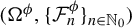
 Moreover, (1.3) naturally induces a filtered space
$(\Omega ^\phi ,\{{\mathcal {F}}_n^\phi \}_{n\in \mathbb N_0})$
 and a family of probability measures
$\{\mathbb P_x^\phi \}_{x \in E_Y}$
 which makes
$X_n^\phi $
 a Markov process (see [Reference Rogers and Williams68, §III.7] for such a construction). Finally, we denote by
$\mathbb E_x$
 and
$\mathbb E_x^\phi $
 the expectation with respect to
$\mathbb P_x$
 and
$\mathbb P_x^\phi $
 , respectively.
Under an irreducibility condition of
$X_n$
 on Y [Reference Castro, Lamb, Olicón-Méndez and Rasmussen19], the process almost surely escapes this set, implying that the system’s long-term behaviour is characterized by a stationary delta measure sitting on the cemetery state. To understand the dynamics of the process before escaping from Y, one generalizes the notion of stationary measures to that of quasi-stationary measures [Reference Breyer and Roberts15, Reference Cattiaux, Collet, Lambert, Martínez, Méléard and San Martín20, Reference Collet, Martínez and Schmitt28, Reference Darroch and Seneta32].
Definition 2.1. Given a bounded and measurable function
$\phi :Y\to \mathbb R$
 , we say that a Borel probability measure
$\mu $
 on Y is a quasi-stationary measure of the weighted Markov process
$X_n^\phi $
 if

and
$\unicode{x3bb} ^\phi =\int _Y e^{\phi (x)}\mathbf P (x, Y)\mu (d x)>0$
 is the growth rate of
$\mu $
 for
$X_n^\phi $
 on Y. Observe that when
$\phi =0$
 , we recover the classical definition of quasi-stationary measure [Reference Collet, Martínez and San Martín27, Definition 2.1].
Remark 2.2. Note that in the usual setting of absorbed Markov processes with no weight function, i.e.
$\phi = 0$
 , and only hard killing,
$\unicode{x3bb} ^\phi \leq 1$
 is called the survival rate and denotes the probability that the process is not killed in the next iterate when distributed according to
$\mu $
 .
We recall that quasi-stationary measures are not the relevant measures to consider when studying conditioned Birkhoff averages [Reference Breyer and Roberts15, Reference Castro, Lamb, Olicón-Méndez and Rasmussen19, Reference Champagnat and Villemonais22, Reference Darroch and Seneta32], as these measures do not perceive how likely it is for a point to remain indefinitely in Y. Instead, this information is provided by the so-called quasi-ergodic measure.
Definition 2.3. A probability measure
$\nu $
 on Y is a quasi-ergodic measure of the
$e^\phi $
 -weighted Markov process
$X_n^\phi $
 if for any bounded measurable function
$h:Y\to \mathbb R$
 , it holds that

If
$X_n^\phi $
 has both hard and soft killing, then for every
$n \in \mathbb N$
 ,

where
$S_n \phi := \sum _{i=0}^{n-1} \phi \circ X_i$
 is the Birkhoff sum.
While showing the existence of quasi-stationary measures relates to solving an eigenfunctional equation and can be approached using fixed point arguments (see [Reference Oikhberg and Troitsky63, Theorem 4] and [Reference Collet, Martínez and San Martín27, Proposition 2.10]), this is not the case for quasi-ergodic measures, and proving their existence and uniqueness is not straightforward. Indeed, this involves characterizing the non-trivial limit of a conditional expectation that requires rigorous techniques in functional analysis and probability theory [Reference Castro, Lamb, Olicón-Méndez and Rasmussen19, Reference Champagnat and Villemonais22, Reference Zhang, Li and Song86]. We devote the Appendix A to address this question in our setup.
From here onwards, let
$(M,\langle \cdot , \cdot \rangle )$
 be an orientable Riemannian compact manifold, possibly with boundary and let
$U\subset M$
 be an open subset. Without loss of generality, we may assume that M is embedded in an orientable boundaryless compact manifold E of the same dimension and endowed with a Riemannian metric whose restriction to M coincides with
$\langle \cdot ,\cdot \rangle $
 (in the case that M is without boundary, we assume that
$E=M$
 ). Since this will be clear by context, we may also write the Riemannian metric of E as
$\langle \cdot ,\cdot \rangle $
 . The manifold E should be thought of as an ambient space for M and a mere theoretical artefact since it does not play a major role in applications, while U may be interpreted as an open hole in the system.
Notation 2.4. Throughout this paper, we use the following notation.
-
(i) Given $x \in E$
and
$v\in T_x E$
, define
$\|v\|_x := \sqrt {\langle v,v\rangle _x}$
as the natural norm on
$T_x M$
. -
(ii) We denote by $\mathrm {dist}(\cdot , \cdot )$
the distance on E induced by the Riemannian metric
$\langle \cdot ,\cdot \rangle $
. -
(iii) As usual, we write $\rho $
for a Borel measure on E induced by a smooth volume form
$V_{E}$
compatible with
$\langle \cdot ,\cdot \rangle $
. -
(iv) We denote by ${\mathcal {C}}^k(E)$
the space of continuous functions with k continuous derivatives on E and use
${\mathcal {M}}(E)$
to denote the space of signed Borel finite measures on an E. Given a non-negative measure
$\rho \in {\mathcal {M}}(E)$
, we denote by
$L^k(E, \rho )$
the space of functions with finite kth
$\rho $
-moment (although
$\rho $
may be omitted when it is the reference measure). Additionally,
${\mathcal {C}}^k_+(E), L^k_{+}(E)$
and
${\mathcal {M}}_+(E)$
denote the respective subsets of non-negative functions and measures on E. -
(v) Given a ${\mathcal {C}}^1$
function
$G:E\to E$
and
$x\in E,$
we denote its determinant by $$ \begin{align*}\det d G(x) = \frac{V_E(G(x))(d G(x)v_1,\ldots, d G(x) v_{\dim E})}{V_E(x)(v_1,\ldots,v_{\dim E})} \end{align*} $$for any (and therefore all) orthonormal basis $\{v_1,\ldots ,v_m\}$
of
$T_x M.$
-
(vi) Given a set $A\subset E$
, we denote its closed neighbourhood of radius
$\delta>0$
by
$A_\delta = \overline {B_\delta (A)}:= \{x \in E;\,\mathrm {dist}(x, a) \leq \delta \text { for some } a \in A\}$
.


2.1 The deterministic dynamics
Let
$T: E\to E$
 be a map such that
$T|_{E\setminus \partial }$
 is
${\mathcal {C}}^2$
 for a suitable choice of
$\partial $
 , e.g.
$\partial $
 may be an open subset
$U \subset M \subset E$
 , where the process is killed or an artificial cemetery state in the absence of hard killing. For an invariant set
$\Lambda $
 as in (1.1), that is,

we consider the following hypothesis.
Hypothesis H1. There exists a compact T-invariant set
$\Lambda \subset E$
 that is uniformly hyperbolic expanding, i.e. there exists
$r>0$
 such that for all
$x \in \Lambda $
 ,

and there exists a neighbourhood V of
$\Lambda $
 in E such that
$T^{-1}(\Lambda ) \cap V = \Lambda $
 . We call
$\Lambda $
 a (uniformly expanding) repeller.
Remark 2.5. Observe that if there exist
$C>0$
 and
$r>0$
 such that

for all
$x\in \Lambda $
 and every
$n\ge 1$
 , then (2.1) holds after a suitable change of the Riemannian metric on M (see [Reference Shub77, Proposition 4.2]).
Uniformly expanding sets admit a well-known ‘spectral’ or ‘dynamical decomposition’ [Reference Hasselblatt and Katok49, Theorem 19.3.6], providing the fundamental sets on which we shall perform our local analysis of conditioned stochastic stability. We denote these by
$R^i, i = 1, \ldots , k$
 , and recall that they are given by the following result.
Lemma 2.6. Let T and
$\Lambda $
 satisfy Hypothesis H1 and consider the set

Then, there exists a (finite) partition of R in non-empty compact sets
$R^{i,j},$
 with
$1\leq i \leq k$
 and
$1\leq j \leq m(i)$
 such that:
-
(1) $R^{i} = \bigcup _{j=1}^{m(i)} R^{i,j}$
is a T-invariant set for every i; -
(2) $T(R^{i,j}) = R^{i,j+1\ (\mathrm {mod}\ m(i))}$
for every
$i,j$
; -
(3) $T:R^i\to R^i$
is uniformly hyperbolic and topologically transitive; and -
(4) each $T^{m(i)}:R^{i,j}\to R^{i,j}$
is uniformly hyperbolic and topologically exact.


Furthermore, the number k, the numbers
$m(i)$
 and the sets
$R^{i,j}$
 are unique up to renumbering.
Proof. See, for example, [Reference Hasselblatt and Katok48, Theorem 18.3.1] or [Reference Viana and Oliveira82, Theorem 11.2.15].
Throughout, we let
$\phi : M \to \mathbb R$
 be a Hölder function, which we may call the weight function, and say that the triple
$(T,\phi ,\Lambda )$
 satisfies Hypothesis H1, although
$\phi $
 does not play a role in this assumption. We recall in the following theorem a well-known result of Ruelle [Reference Ruelle72, Lemma 1.4] (see also [Reference Ruelle71, Chs. 7.26–7.31]) that provides the existence and uniqueness of equilibrium states associated with the potential
$\psi = \phi - \log |\!\det d T|$
 on each
$R^i, i = 1, \ldots , k$
 (recall §1.2), for triples
$(T, \phi , R^i)$
 satisfying Hypothesis H1.
Theorem 2.7. (Ruelle)
Let T satisfy Hypothesis H1. Let
$R^1,\ldots , R^k$
 be as in Lemma 2.6 and fix
$i\in \{1,\ldots ,k\}$
 . For every
$\alpha $
 -Hölder potential
$\psi : R^i\to \mathbb {R}$
 ,
$\alpha> 0$
 , consider the operator

and denote by
${\mathcal {L}}^*:{\mathcal {M}}(R^i) \to {\mathcal {M}}(R^i)$
 its dual (recall Notation 2.4). Then, there exist a unique
$m\in {\mathcal {C}}_+^0(R^i)$
 ,
$\gamma \in {\mathcal {M}}_+(R^i)$
 and
$\unicode{x3bb}>0$
 satisfying:
-
(1) $\ker (\mathcal {L} - \unicode{x3bb} ) = \mathrm {span}(m)$
; -
(2) $\ker (\mathcal {L}^* -\unicode{x3bb} ) = \mathrm {span}(\gamma )$
and
$\int _{R^i} m(x) \gamma (dx) = 1$
; and -
(3) $\log \unicode{x3bb} = \log r(\mathcal {L}) = h_{\nu } + \int \phi (x)\nu (d x)$
, where
$\nu (d x) = m(x) \gamma (d x)$
.


In this context,
$\nu $
 is the unique T-invariant equilibrium state for the potential
$\psi $
 on
$R^i$
 .
In the study of local conditioned stochastic stability, we shall set
$\Lambda = R^i$
 for a fixed
$i \in \{1, \ldots , k\}$
 and consider small random perturbations of the dynamics as long as the process remains in a suitable
$\delta $
 -neighbourhood of this invariant set, i.e.
$\partial = M \setminus R^i_\delta $
 . As mentioned above, Theorem 2.7 provides the existence and uniqueness of equilibrium states, each associated to a particular Hölder potential
$\psi $
 , on every repeller
$R^i$
 ,
$i \in \{1, \ldots , k\}$
 . These equilibrium states are the objects we prove to be conditioned stochastically stable.
The study of global conditioned stochastic stability, as motivated in §1, begins by considering a more general open cemetery state, hole or absorbing region,
$U \subset M$
 . The set of points that never enters this region U under the dynamics, similarly to (1.1), is given by

The main working assumption in this global setting ensures that
$T|_{\Lambda }$
 , with
$\Lambda $
 as in (2.3), admits a unique equilibrium state for each
$\alpha $
 -Hölder weight function
$\phi $
 . This is detailed in the following hypothesis.
Hypothesis H2. We say that
$(T, \phi , \Lambda )$
 satisfies Hypothesis H2 for the open hole U if the following hold:
-
(i) $\Lambda := \bigcap _{n \geq 0} T^{-n}(M\setminus U)$
is a uniformly expanding set; -
(ii) T admits a unique equilibrium state for the potential $\psi = \phi - \log |\!\det d T|$
on
$\Lambda ;$
and -
(iii) there exists $\delta>0$
such that
$T^{-1}(\Lambda _\delta )\cap M_\delta \subset \Lambda _\delta $
and
$M_\delta \setminus M$
has no T-invariant subsets.


We set the cemetery state
$\partial := U \cup (E \setminus M_\delta )$
 .
Remark 2.8. If
$M = [0,1]$
 , items (i) and (ii) of Hypothesis H2 are equivalent to the Axiom A (see e.g. [Reference de Melo and van Strien35, Ch. 3.2.b]).
Remark 2.9. In the case where M is a manifold without boundary, then
$M_\delta = M = E$
 and
$\Lambda _\delta \subset M.$
 Observe that item (iii) always holds true in dimension one. In fact, recall that
$M \subset E$
 , where E acts as an ambient space. With item (iii), we ensure that there are no invariant subsets near M, which could trap the perturbed dynamics.
2.2 The random perturbations
When T satisfies Hypothesis H2, given a finite
$\varepsilon>0$
 , we consider the random perturbation of the form
$F_\varepsilon :[-\varepsilon ,\varepsilon ]^m \times E\to E, $
 where
$F_\varepsilon (\omega , \cdot ) \in {\mathcal {C}}^2(E\setminus U; E)$
 and
$\partial _{\omega } F_\varepsilon (\omega , x)$
 is surjective for all
$\omega \in [-\varepsilon ,\varepsilon ]^m$
 . Moreover, we assume that
$\mathrm {dist}_{{\mathcal {C}}^2}(F_\varepsilon (\omega ,\cdot ), T)\leq {C}\|\omega \|$
 for some
$C>0$
 , where
$\mathrm {dist}_{{\mathcal {C}}^2}$
 denotes the metric on
${\mathcal {C}}^2(E \setminus U,E)$
 , which generates the
${\mathcal {C}}^2$
 -Whitney topology [Reference Palis and de Melo64, Ch. 1.2]. In particular, surjectivity of
$\partial _\omega F_\varepsilon (\omega , x)$
 implies
$m \geq \dim E$
 . We note that this type of random perturbation is natural and commonly considered [Reference Alves, Araújo and Vásquez2, Reference Araújo3, Reference Baladi and Viana7, Reference Benedicks and Viana9, Reference Benedicks and Young10].
Let
$\Omega _\varepsilon := ([-\varepsilon ,\varepsilon ]^m)^{\mathbb N}$
 be the space of semi-infinite sequences of elements in
$[-\varepsilon ,\varepsilon ]^m$
 endowed with the probability measure
$\mathbb {P}_\varepsilon := (\text {Leb}|_{[-\varepsilon , \varepsilon ]^m}/(2\varepsilon )^m)^{\otimes \mathbb {N}}$
 and let
$\mathbb {E}_\varepsilon $
 denote the corresponding expectation with respect to
$\mathbb {P}_\varepsilon $
 . For every
$\omega \in \Omega _\varepsilon $
 ,
$\omega = (\omega _0 \omega _1 \cdots )$
 , we define
$T_{\omega }(x):= T_{\omega _0}(x) := F_\varepsilon (\omega _0,x)$
 and
$T^n_\omega (x) := T_{\omega _{n-1}} \circ \cdots \circ T_{\omega _{n}}(x)$
 for every
$n \in \mathbb N$
 , e.g. we may consider by abuse of notation
$X_{n+1} = F_{\omega _n}(X_n)$
 for an independent and identically distributed (i.i.d.) sequence of random variables
$(\omega _n)_{n \geq 0}$
 following a uniform law on
$[-\varepsilon ,\varepsilon ]^m$
 .
As mentioned in §1, Corollary B1 applies to suitable
$\delta $
 -neighbourhoods of each repeller
$R^i$
 ,
$1 \leq i \leq k$
 , in the dynamical decomposition of Lemma 2.6. In particular, from the definition of
$F_\varepsilon $
 , we may consider a suitable
$\delta $
 -neighbourhood of this decomposition still consisting of k elements, which almost surely do not communicate under a single iteration of the dynamics. This is summarized in the following lemma, whose proof we omit as it follows from standard arguments.
Lemma 2.11. Under Hypothesis H1, for every
$\delta> 0$
 small enough, there exists
$\varepsilon _0 := \varepsilon _0(\delta )> 0$
 such that for every
$0 \leq \varepsilon \leq \varepsilon _0$
 , we have that:
-
(1) $R_\delta = R^1_\delta \sqcup \cdots \sqcup R_\delta ^k$
; and -
(2) $\sup _{x\in R^i_\delta }\mathbb {P}_\varepsilon [\omega \in \Omega _\varepsilon ;\ T_\omega (x) \in R^j_\delta ] = 0$
for every
$i\neq j \in \{1,\ldots , k\}.$



To establish the existence of quasi-ergodic measures, we exploit the properties of a stochastic analogue to (the dual of) Ruelle’s transfer operator
${\mathcal {L}}$
 presented in Theorem 2.7. This may become clearer in the following section, particularly after introducing Notation 3.3. For each
$i \in \{1, \ldots , k\}$
 and every
$\alpha $
 -Hölder function
$\phi :R^i_\delta \to \mathbb R$
 (see Notation 2.4(vi)), we define the annealed Koopman operator

for f in a suitable domain. In other words, for the absorbing and weighted Markov process
$X^{\varepsilon ,\phi }$
 starting at
$x \in \mathbb R^i_\delta $
 and defined by

with
$\partial $
 the complement of
$R^i_\delta $
 and such that
$X_n^{\varepsilon ,\phi } = \partial $
 implies
$X_{n+1}^{\varepsilon ,\phi } = \partial $
 for all
$n \geq 1$
 , we have that

For the global picture, we consider Hölder weights
$\phi :M \to \mathbb R$
 and define the (global) annealed Koopman operator given by

for f in a suitable domain, where U is the open hole from Hypothesis H2.
2.3 Main results
The main results of this paper are as follows.
Theorem 2.12. Assume Hypothesis H1 and let
$\delta>0$
 be small enough. Given
$1\leq i\leq k$
 and an
$\alpha $
 -Hölder function
$\phi :R^i_\delta \to \mathbb {R}$
 , the following properties hold for
$\varepsilon>0$
 sufficiently small:
-
(1) the $e^\phi $
-weighted Markov process
$X_n^{\varepsilon ,\phi }$
admits a unique quasi-stationary measure
$\mu _\varepsilon $
on
$R_\delta ^i$
such that
$\Lambda \subset {\mathrm {supp}}\, \mu _\varepsilon $
; -
(2) let $\unicode{x3bb} _\varepsilon $
be the growth rate of
$X_n^{\varepsilon ,\phi }$
on
$R_\delta ^i$
, then
$\unicode{x3bb} _\varepsilon $
is equal to the spectral radius of
$\mathcal {P}_\varepsilon :L^\infty (R^i_\delta ,\rho ) \to L^\infty (R^i_\delta ,\rho )$
and
$\log (\unicode{x3bb} _\varepsilon ) \to P(T,\phi -\log |\!\det d T|, R^i)\ \text {as}\ \varepsilon \to ~0;$
-
(3) the operator ${\mathcal {P}_\varepsilon : L^{\infty }(R_{\delta }^i, \rho ) \to L^{\infty }(R_{\delta }^i, \rho )}$
admits a unique positive eigenfunction
$g_\varepsilon \in L^{\infty }(R_{\delta }^i, \rho )$
associated with the eigenvalue
$\unicode{x3bb} _\varepsilon $
; -
(4) the $e^\phi $
-weighted process
$X_n^{\varepsilon ,\phi }$
on
$\{g_\varepsilon>0\}$
admits a unique quasi-ergodic measure
$\nu _\varepsilon (d x)$
on
$\{g_\varepsilon> 0\}$
; -
(5) $\nu _\varepsilon (d x)\to \nu _0(d x)$
in the weak
$^*$
topology as
$\varepsilon \to 0$
and -
(6) $\nu _0$
is the unique T-invariant equilibrium state for the potential
$\phi -\log |\!\det d T|$
on
$R^i$
.


If the measure
$\nu _0$
 is mixing for the map
$T: R^i\to R^i$
 , then the measure
$\nu _\varepsilon $
 is also a quasi-ergodic measure of the
$e^\phi $
 -weighted Markov process
$X_n^\varepsilon $
 on
$R_\delta ^i$
 .
The local Theorem 2.12 under Hypothesis H1 is a version of the following global theorem under Hypothesis H2.
Theorem 2.13. Assume Hypothesis H2, let
$\nu _0$
 be the unique T-invariant equilibrium state for the potential
$\phi -\log |\!\det d T|$
 on
$\Lambda $
 and
$\delta>0$
 be small enough. Given an
$\alpha $
 -Hölder function
$\phi :M_\delta \setminus U \to \mathbb {R}$
 , the following properties hold for
$\varepsilon>0$
 sufficiently small:
-
(1) the $e^\phi $
-weighted Markov process
$X_n^{\varepsilon ,\phi }$
admits a unique quasi-stationary measure
$\mu _\varepsilon $
on
$M_\delta \setminus U$
such that
$\mathrm {supp}\, \nu _0\subset {\mathrm {supp}}\, \nu $
; -
(2) let $\unicode{x3bb} _\varepsilon $
be the growth rate of
$X_n^{\varepsilon ,\phi }$
on
$M_delta\setminus U$
, then
$\unicode{x3bb} _\varepsilon $
is equal the spectral radius of
$\mathcal {P}_\varepsilon :L^\infty (M_\delta \setminus U) \to L^\infty (M_\delta \setminus U) $
and
$\log (\unicode{x3bb} _\varepsilon ) \to P(T,\phi -\log |\!\det d T|, \Lambda )$
as
$\varepsilon \to 0;$
-
(3) the operator $\mathcal {P}_\varepsilon : L^{\infty }(M_\delta \setminus U, \rho ) \to L^{\infty }(M_\delta \setminus U, \rho )$
admits a unique positive eigenfunction
$g_\varepsilon \in L^{\infty }(M_\delta \setminus U,\rho )$
associated with the eigenvalue
$\unicode{x3bb} _\varepsilon $
; -
(4) the $e^\phi $
-weighted process
$X_n^{\varepsilon ,\phi }$
on
$\{g_\varepsilon>0\}$
admits a unique quasi-ergodic measure,
$\nu _\varepsilon (d x)$
on
$\{g_\varepsilon> 0\} \cap {\mathrm {supp}}\, \mu _\varepsilon $
and -
(5) $\nu _\varepsilon (d x) \to \nu _0(d x)$
in the weak
$^*$
topology as
$\varepsilon \to 0$
.


If
$\nu _0$
 is mixing for the map
$T: R\to R$
 , then the conclusions of the above theorem remain true when changing the set
$\{g_\varepsilon>0\}\cap {\mathrm {supp}}\, \mu _\varepsilon $
 by
$M_\delta \setminus U$
 . Additionally, if
$\nu _0$
 is mixing and
${\mathrm {supp}}\, \nu _0 \subset \mathrm {Int}(M\setminus U)$
 , then property (4) is also true on the set
$M \setminus U$
 .
2.4 Examples
Let us provide three examples to illustrate Hypotheses H1 and H2, along with the main results obtained from Theorems 2.12 and 2.13.
2.4.1 The logistic map
Consider the Markov process
$X_{n+1}^\varepsilon = T(X_{n}^\varepsilon ) + \omega _n$
 ,
$n \in \mathbb {N},$
 with
$T(x) = ax(1-x)$
 and
$\omega _n \sim \text {Unif}(-\varepsilon , \varepsilon )$
 . Fix
$a = 3.83$
 so that the deterministic dynamical system (with
$\varepsilon = 0$
 ) has an almost sure global three-periodic attractor [Reference Crutchfield, Farmer and Huberman31, Reference Sato, Doan, Lamb and Rasmussen74], i.e. Lebesgue almost every initial condition in
$[0,1]$
 is attracted to the unique three-periodic hyperbolic attractor
${\mathcal {A}} = \{p, T(p) , T^{2}(p)\}$
 , with
$p \approx 0.1456149$
 (see Remark 2.8).
The dynamical decomposition of Lemma 2.6 yields two invariant sets: the origin
$R^1 =\{0\}$
 and a hyperbolic Cantor set
$R^{2}$
 consisting of the closure of all periodic points in
$(0,1)$
 that are not in the basin of attraction
$B(T)$
 of
${\mathcal {A}}$
 [Reference Smale and Williams80]. Let
$\Lambda := [0,1] \setminus B(T)$
 and
$U \supset {\mathcal {A}}$
 be a small enough neighbourhood of the attractor such that
$U \cap \Lambda = \emptyset $
 . We consider the family of
$\alpha $
 -Hölder weight functions
$\phi _t:[0,1] \to \mathbb R, x \mapsto (-t+1)\log |T'(x)|$
 for
$t \geq 0$
 . Recall that an equilibrium state
$\nu _i$
 associated with the potential
$\phi _t - \log |a(1-2x)|$
 for T on
$R^i$
 is a measure maximizing

where
$h_\mu $
 is the metric entropy and
$\mu \in {\mathcal {I}}(T,R^i)$
 the set of T-invariant measures on
$R^i$
 .
It is well known that
$\Lambda $
 is a hyperbolic (uniformly expanding) invariant set [Reference de Melo and van Strien35] and T admits a unique equilibrium state associated with the potential
$\phi _t(x) -\log |T'(x)|$
 on
$\Lambda $
 (see e.g. [Reference Viana and Oliveira82, Chs. 11 and 12]). Therefore, Hypothesis H2 is satisfied and we can apply the theory developed above. For
$R^1$
 , it is clear that
$\nu _1 = \delta _0$
 and
$P(T, \phi _t - \log |T'|, R^1) = -t \log |a|$
 . For
$R^2$
 ,

since
$-\!\log |a(1-2x)|$
 reaches its minimum at
$0$
 and
$h_{\nu _2} = (1 + \sqrt {5})/2$
 (see [Reference Smale and Williams80] for precise details). Therefore,

with
$\mathcal {P}_\varepsilon : L^{\infty }([0,1] \setminus U) \to L^{\infty }([0,1] \setminus U)$
 the global annealed Koopman operator. It follows from Theorem 2.13 that the unique equilibrium state sits on the invariant Cantor set repeller
$R^2$
 and can be approximated by quasi-ergodic measure
$\nu _\varepsilon $
 of the
$\phi _t$
 -weighted Markov process
$X_n^\varepsilon $
 on a neighbourhood of
$R^2$
 , as
$\varepsilon \to 0$
 .
For the particular choice of
$t = 1$
 , i.e.
$\phi _{t=1} = 0$
 , the system is no longer spatially weighted and we recover the so-called ‘natural measure’ of the repeller [Reference Kantz and Grassberger51]. We note that the relationship between limiting quasi-ergodic measures and natural measures in the case of the zero weighting was previously discussed in [Reference Bassols-Cornudella and Lamb8] for this example.
Finally, consider the potential
$\phi _0(x)= \log |T'|$
 . The topological pressure of the deterministic system on
$\Lambda $
 is given by
$P(T, 0 , \Lambda ) = h_{\nu }(T),$
 where
$\nu $
 is the unique equilibrium state. Since this measure maximizes
$P(T, 0, \Lambda )$
 , it coincides with the measure of maximal entropy of the system.
2.4.2 The complex quadratic map
Similarly to the previous example, let us consider random perturbations of iterates of the complex quadratic map
$p_c(z) = z^2 + c$
 ,
$c \in \mathbb {C}$
 , acting on the Riemann sphere
$\widehat {\mathbb C} = \mathbb C \sqcup \{\infty \}$
 . As before, we study the Markov process
$X_{n+1}^\varepsilon = p_c(X_n^\varepsilon ) + \omega _n$
 , where
$\{\omega _n\}_n$
 are i.i.d. random variables uniformly distributed on
$\{a+i b\in \mathbb C;\, (a,b)\in [-\varepsilon ,\varepsilon ]^2\}$
 , with
$\varepsilon>0$
 small enough.
Consider the Julia set
$ J \subset \widehat {\mathbb {C}} $
 associated with the polynomial
$ p_c $
 . Recall that J is the closure of the set of repelling periodic points [Reference Milnor62, Theorem 11.1]. The set
$ J $
 is non-empty, compact and totally invariant, meaning that
$ J = p_c(J) = p_c^{-1}(J) $
 (see [Reference Milnor62, Lemma 3.1]). Now, let
$ c $
 be a hyperbolic complex number within the Mandelbrot set, which ensures that J is hyperbolic, that is, J is connected and satisfies
$ \|p_c'(z)\| = \|2z\|> 1 $
 for every
$ z \in J $
 .
In this context, it is readily verified that
$p_c$
 admits a finite attractor
$\mathcal {A}\subset \mathbb C$
 . Moreover, for any
$\alpha $
 -Hölder weight function
$\phi : \mathbb {C} \to \mathbb {R}$
 ,
$p_c$
 satisfies Hypothesis H2 with
$T= p_c$
 ,
$\Lambda = J$
 and
$E= M= \widehat {\mathbb C}$
 . Furthermore, notice that the unique equilibrium state of
$p_c$
 for the potential
$\phi - \log |\!\det d p_c|$
 on J is mixing.
Finally, from Theorem 2.13, for any
$\alpha $
 -Hölder potential
$\psi : \widehat {\mathbb C} \to \mathbb {R}$
 , the unique
$p_c$
 -invariant equilibrium state for the potential
$\psi $
 on J can be approximated in the weak
$^*$
 topology by quasi-ergodic measures of the
$(\psi + \log |\!\det d p_c|)$
 -weighted Markov process
$X_n^\varepsilon $
 on
$\widehat {\mathbb {C}}\setminus U$
 , where U is a neighbourhood of
$\mathcal {A}$
 such that
$U\cap J = \emptyset .$

2.4.3 The Boole map
Consider the Boole map
$T:\mathbb S^1 \to \mathbb S^1$
 on the circle given by [Reference Boole12]

which consists of two branches. This map is not uniformly expanding since
$T'(0) =1$
 and, hence, does not satisfy either of the Hypotheses H1 or H2 for
$\partial = \emptyset $
 . Nevertheless, this is the only neutral fixed point and T is expanding elsewhere.
Consider the open hole
$U_s = \{x\in \mathbb S^1;x\in [0,s)\ \text {or }x\in (1-s,1] \}$
 for
$s\in (0,1/8)$
 , and let

be the set of points in
$\mathbb S^1 \setminus U_s$
 that are never mapped into
$U_s$
 . Observe that for each
$s\in (0,1/8)$
 ,
$\Lambda ^s\neq \emptyset $
 , since it is easy to verify that there exists a
$2$
 -periodic orbit lying in
$\mathbb S^1 \setminus U_s$
 for every
$s\in (0,1/8)$
 . Moreover,
$\Lambda ^s \subset \mathbb S^1\setminus U_s$
 and, therefore, T is uniformly hyperbolic when restricted to
$\Lambda _s$
 . Therefore,
$(T, \phi , \Lambda ^s)$
 satisfies Hypothesis H1 for any Hölder weight function
$\phi $
 for any
$s\in (0,1/8)$
 and
$E = V = \mathbb S^1.$

We show that for suitable
$\phi :\Lambda \to \mathbb R$
 and for
$\mathrm {Leb}$
 -a.e.
$s\in (0,1/8)$
 ,
$(T,\phi ,\Lambda ^s)$
 satisfies Hypothesis H2. It is well known (see e.g. [Reference Aaronson1, Reference Bonanno, Giulietti and Lenci11, Reference Zweimüller88]) that T admits an infinite invariant
$\mu \ll \mathrm {Leb}$
 on
$\mathbb S^1$
 and that T is
$\mu $
 -conservative, that is, for any measurable set
$\mu (A)>0$
 ,
$\mu $
 -a.e.
$y\in \mathbb S^1$
 returns to A so that
$\# \{n\in \mathbb N; T^n(y)\in A\} = \infty .$
 In particular, the set

has full
$\mu $
 -measure, that is,
$\mu (\mathbb S^1 \setminus B) = 0$
 . Define the set of parameters

From (2.4), it follows that
$\text {Leb}(S) = 1/8.$

We therefore obtain that for each
$s\in \mathbb S$
 ,
$\Lambda ^s\cap \overline {U}_s = \emptyset $
 , yielding Hypothesis H2(iii). Since
$T:\Lambda _s\to \Lambda _s$
 is uniformly hyperbolic, Hypothesis H2(i) is also satisfied. The last item to verify is part (ii) which, for each
$s \in \mathbb S$
 , already holds generically for
$\phi \in {\mathcal {C}}^\alpha $
 ,
$\alpha> 0$
 .
As in the previous examples, we obtain conditioned stochastic stability of equilibrium states on
$\Lambda ^s$
 .
3 Some direct consequences of Hypothesis H1
This section contains several dynamical and topological results that follow from Hypothesis H1 rather immediately, and are exploited later in the paper. We also formally introduce the transfer operators
$\mathcal {L}_\varepsilon $
 and its dual
$\mathcal {P}_\varepsilon $
 , prove that
$\mathcal {P}_\varepsilon $
 is strong Feller, and obtain that their iterates are compact.
Lemma 3.1. Let T satisfy Hypothesis H1. Consider
$\delta>0$
 small enough. Then, there exists
$\varepsilon _0 := \varepsilon _0(\delta )$
 and
$\sigma _1 := \sigma _1(\delta ) < 1$
 such that for every
$x,y \in \Lambda _\delta $
 satisfying
$T(y) = x$
 and for every
$0<\varepsilon < \varepsilon _0$
 , there exists a
${\mathcal {C}}^2$
 function
$h:[-\varepsilon ,\varepsilon ]^m\times C_x \to E$
 , where
$C_x$
 is the connected component of x in
$\Lambda _\delta $
 , with the following properties holding for every
$\omega \in \Omega _\varepsilon $
 :
-
(1) the map $z\mapsto h(\omega ,z)$
is a diffeomorphism onto its image; -
(2) $T_\omega \circ h(\omega ,z) = z$
for every
$z\in C_x$
and
$h(0,x)= y;$
-
(3) $\mathrm {dist}(h(\omega ,x_1), h(\omega ,x_2)) \leq \sigma _1\ \mathrm {dist}(x_1,x_2)$
for every
$x_1,x_2\in C_x$
; and -
(4) there exists $K_0 = K_0(\delta )>0$
uniform on
$\varepsilon \in (0,\varepsilon _0)$
,
$x\in \Lambda _\delta $
and
$y\in T^{-1}(x)\cap \Lambda _\delta $
, such that
$ \sup \{\|\partial _\omega h(\omega ,z)\| ;\ \omega \in \Omega _\varepsilon ,\ z\in C_x\}\leq K_0$
.


All statements in this lemma also hold true replacing
$\Lambda _\delta $
 by
$R^i_\delta $
 ,
$1 \leq i \leq k$
 .
Proof. Take
$\delta _0,\varepsilon _0>0$
 small enough such that

and such that the exponential map
$\exp _{z}: B_{\delta _0}(0) \subset T_z E\to E$
 is well defined for every
$z\in \Lambda _{\delta _0}$
 .
Observe that there exists
$\delta _2>0$
 such that for
$\varepsilon _0>0$
 small enough and for every
$\omega \in [-\varepsilon _0,\varepsilon _0]^m$
 , if
$\mathrm {dist}(x_1,x_2)<\delta _2$
 , then we obtain that
$\mathrm {dist}(T_\omega (x_1),T(x_2))<\delta _0.$
 Consider the map

Observe that
$G(0,x,y)= 0$
 . Since
$ \partial _{y} G(0,x,y)$
 is surjective, by means of the implicit function theorem, there exists a
${\mathcal {C}}^2$
 function
$h:[-\varepsilon _0(y),\varepsilon _0(y)]^m\times B_{\tau (y)}(x) \to E$
 such that
$T_{\omega } (h(\omega ,z)) = z$
 for every
$z\in B_{\tau (y)}(x)$
 and
$h(0,x)=y$
 . Notice, as well, that
$\varepsilon _0(y),\tau (y)$
 can be taken uniformly since
$\Lambda _\delta $
 is compact and, therefore, we can
${\mathcal {C}}^2$
 -extend h to the domain
$[-\varepsilon ,\varepsilon ]^m\times C_x.$
 Finally, from (3.1), we obtain that the function h satisfies all the desirable properties. Replacing
$\Lambda _\delta $
 by
$R_\delta ^i$
 follows from Lemma 2.11(2).
Lemma 3.2. Let T satisfy Hypothesis H1. There exists
$\delta _0> 0$
 small enough satisfying Lemma 2.11 such that:
-
(1) there exists $\sigma _0:= \sigma _0(\delta _0) \in (0,1)$
such that
$T^{-1}(\Lambda _\delta ) \cap \Lambda _\delta \subset \Lambda _{\sigma _0 \delta }$
for all
$0<\delta < \delta _0$
.


Moreover, there exists
$\varepsilon _0 := \varepsilon _0(\delta )$
 satisfying Lemma 3.1 such that for every
$0 < \varepsilon < \varepsilon _0$
 , we have that:
-
(2) there exists $\sigma := \sigma (\delta ,\varepsilon ) \in (0,1)$
such that
$T^{-1}_\omega (\Lambda _\delta ) \cap \Lambda _\delta \subset \Lambda _{\sigma \delta }$
for every
$\omega \in ~\Omega _\varepsilon $
; and -
(3) for all $x,y$
lying in the same connected component of
$\Lambda _\delta $
and all
$\omega \in \Omega _\varepsilon $
, we have
$\#\{T^{-1}(x)\cap \Lambda _\delta \} = \#\{T_\omega ^{-1}(y)\cap \Lambda _\delta \}.$


All statements in this lemma also hold true replacing
$\Lambda _\delta $
 by
$R^i_\delta $
 ,
$i \in \{1, \ldots , k\}$
 .
Proof. We prove statement (3.2). Take
$\delta _0$
 and
$\varepsilon _0$
 small enough such that
$\|d T_{\omega _0}(x)^{-1}|_{\Lambda _{\delta _0}}\| <1$
 for all
$\omega _0\in [-\varepsilon _0,\varepsilon _0]^m$
 and
$\Lambda _{2\delta _0}\subset V$
 , where V is as in Hypothesis H1. Let
$0<\delta <\delta _0$
 and
$0<\varepsilon <\varepsilon _0$
 .
Given
$x\in E$
 and
$v\in T_x E$
 such that
$\|v\|_x=1$
 , let
$\gamma _{x,v}:(-\delta _0,\delta _0)\to E$
 be a geodesic on E such that
$\gamma _{x,v}(0) = x$
 and
$\gamma _{x,v}'(0)= v\in T_x E$
 . From Hypothesis H1, the fact that T is a
${\mathcal {C}}^2$
 function and
$\Lambda $
 is compact, we have that
$\gamma _{y,w}(\delta )$
 is well defined for every
$y \in \Lambda $
 and
$w\in T_y E,$
 and that there exists
$r_0>0$
 such that

From the above equation and the fact that
$d T(x)$
 is a surjective linear operator, we obtain that
$T(B_{\delta /(1+r_0)}(y)) \supset B_\delta (T(y))$
 . Take
$y\in \Lambda _\delta $
 , then there exists
$x\in \Lambda $
 ,
$v\in T_x E$
 and
$h\in ~[-\delta ,\delta ]$
 such that
$y = \gamma _{x,v}(h)$
 . Let
$x_1,\ldots ,x_{\ell } \in \Lambda $
 be all pre-images of x. From (3.2), there exist
$h_1,\ldots ,h_\ell \in [-\delta /(1+r_0),\delta /(1+r_0)]$
 and unit vectors
$v_1 \in T_{x_1}E, \ldots , v_{\ell } \in T_{x_\ell } E$
 such that all
$y_i = \gamma _{x_i,v_i}(h_i), 1 \leq i \leq \ell ,$
 are pre-images of y. Note that
$y_i \in \Lambda _{\delta /(1+r_0)}$
 . We claim that these are precisely the only pre-images of y in
$\Lambda _\delta $
 . Suppose there exists
$y' \in \Lambda _\delta \setminus \Lambda _{\delta /(1+r_0)}$
 such that
$T(y') = y$
 . Since
$x \in B_\delta (y)$
 , from (3.2), there is
$h'\in [-\delta /(1+r_0),\delta /(1+r_0)]$
 and
$v'\in T_x E$
 such that
$T(\gamma _{y',v'}(h')) = x$
 . This contradicts Hypothesis H1 as
$\gamma _{y,v}(h') \in \Lambda _{2\delta }\setminus \Lambda \subset V\setminus \Lambda $
 . Therefore,
$T^{-1}(\Lambda _{\delta })\cap \Lambda _\delta \subset \Lambda _{\delta /(1+r_0)}.$
 Set
$\sigma _0 := 1/(1 + r_0)$
 .
We prove statement (3.2). For every
$y\in \Lambda _\delta $
 , let
$\{y_1,\ldots ,y_\ell \}:= T^{-1}(y)\cap \Lambda _\delta $
 . Let
$h_1,\ldots ,h_\ell :[-\varepsilon ,\varepsilon ]^m\times C_y\to E$
 be the inverse branch functions defined in Lemma 3.1 such that
$h_i(0,y)=y_i.$
 Since
$\mathrm {dist}(h_i(\omega ,y), y_i) =\mathrm {dist}(h_i(\omega ,y), h_i(0,y)) < K_0\|\omega \| \leq K_0 \varepsilon $
 and
$y_i\in \Lambda _{\delta /(1+r_0)}$
 from statement (3.2), we obtain that
$h_i(\omega ,y) \in \Lambda _{\delta (K_0\varepsilon + 1/(1 +r_0))}$
 . Choosing
$\varepsilon $
 small enough, there exists
$\sigma \in (0,1)$
 for which
$h_i(\omega ,y) \in \Lambda _{\sigma \delta }$
 for all
$\omega \in \Omega _\varepsilon $
 .
To finish the proof, we show that for
$\varepsilon>0$
 small enough,
$\#\{T^{-1}(x)\cap \Lambda _\delta \} = \#\{T_\omega ^{-1}(x)\cap \Lambda _\delta \} $
 for every
$x\in \Lambda _\delta $
 and
$\omega \in \Omega _\varepsilon .$
 From the construction above, we obtain that
$\#\{T^{-1}(x)\cap \Lambda _\delta \} \leq \#\{T_\omega ^{-1}(x)\cap \Lambda _\delta \}.$
 Suppose for a contradiction that there exist sequences
$\{x_n\}_{n\in \mathbb N}\subset \Lambda _\delta $
 and
$\{\omega _n\}_{n\in \mathbb N}\subset [-\varepsilon _0,\varepsilon _0]^m$
 such that
$\#\{T^{-1}(x_n)\cap \Lambda _\delta \} <\#\{T_{\omega _n}^{-1}(x_n)\cap \Lambda _\delta \}$
 and
$\omega _n\to 0.$
 From the compactness of
$\Lambda _\delta $
 and the pigeonhole principle, the above assumption implies that there exist sequences
$\{y^1_n\}_{n\in \mathbb N}$
 and
$\{y^2_n\}_{n\in \mathbb N}$
 such that: (a)
$y^1_n \neq y^2_n$
 and
$T_{\omega _n}(y_n^1) = T_{\omega _n}(y_n^2)$
 for every
$n\in \mathbb N$
 ; and (b)
$y^1_n,y^2_n\xrightarrow []{n\to \infty } y^* \in \Lambda _\delta $
 . From the continuity of
$(\omega ,x) \mapsto T_\omega (x)$
 , we obtain that
$\mathrm {dist}(T(y_n^1),T(y_n^2))\xrightarrow []{n\to \infty }0$
 , which contradicts the fact that
$d T(y^*)$
 is invertible and completes the proof.
We prove statement (3.2). From the last part in the proof of statement (3.2), we obtain that
$\#\{T^{-1}(x) \cap \Lambda _\delta \} = \#\{T_\omega ^{-1}(x) \cap \Lambda _\delta \}$
 for every
$x\in \Lambda _\delta $
 and
$\omega \in \Omega _\varepsilon $
 for
$\varepsilon $
 sufficiently small. Therefore, it is sufficient to show that the map
$ x\in \Lambda _\delta \mapsto \#\{T^{-1}(x) \cap \Lambda _\delta \}$
 is locally constant. This is a direct consequence of
$\|d T^{-1}(x)\|<1$
 for all
$x\in \Lambda _\delta $
 and the inverse function theorem (see e.g. the proof of [Reference Viana and Oliveira82, Lemma 11.1.4]).
The last statement follows from replacing
$\Lambda _\delta $
 by
$R_\delta ^i$
 in every argument above, and from item (2) of Lemma 2.11. Note that for item (1), we have that
$R^i$
 is open in
$T^{-1}(R^i)$
 (see the proof of [Reference Viana and Oliveira82, Corollary 11.2.16]).
To approximate the equilibrium states in Theorem 2.7 and establish conditioned stochastic stability, we propose using quasi-ergodic measures, which we construct from the principal eigenfunctions of the following annealed transfer operators.
Notation 3.3. For each
$i \in \{1, \ldots , k\}$
 and every
$\alpha $
 -Hölder function
$\phi :R^i_\delta \to \mathbb R$
 , we define the annealed Ruelle–Perron–Frobenius operator

and the annealed Koopman operator

which are well posed from Lemmas 2.11, 3.1 and 3.2. Moreover, given
$x\in R^i_\delta $
 and
$n\in ~\mathbb N$
 , we refer to the measure
${\mathcal {P}}^n_{\varepsilon }(x,\cdot )$
 as the unique measure on
$R_\delta ^i$
 such that
$\mathcal {P}_{\varepsilon }^n(x,A) = \mathcal {P}_{\varepsilon }^n \mathbb {1}_A (x)$
 for every measurable subset A of
$R_\delta ^i.$

Observe that given an
$\alpha $
 -Hölder weight function
$\phi :R^i_\delta \to \mathbb {R}$
 , then
$\mathcal {L}_{\varepsilon }^* = \mathcal {P}_{\varepsilon }$
 . Indeed, for any
$f\in L^1(R^i_\delta )$
 and
$g\in L^\infty (R^i_\delta )$
 , a change of variable shows that (see [Reference Demers, Kiamari and Liverani37, (1.1.1)])

where (if needed) we assume that
$f:E \to \mathbb {R}$
 vanishes outside of
$R^{i}_\delta $
 .
Remark 3.4. Note that the Ruelle–Perron–Frobenius operator
${\mathcal {L}}$
 introduced in Theorem 2.7 differs from the operator
${\mathcal {L}}_\varepsilon $
 since the latter is divided by
$|\!\det d T_\omega |$
 . This causes the correction
$- \log |\!\det d T|$
 for the limiting potential in Theorems 2.12 and 2.13. This choice provides a more interpretable expression for
${\mathcal {P}}_\varepsilon $
 and its eigenfunctions as quasi-stationary measures for the
$e^\phi $
 -weighted Markov process
$X_n^{\varepsilon ,\phi }$
 .
The following proposition establishes that
$X_n^{\varepsilon ,\phi }$
 is a strong Feller absorbing Markov process. This is constantly exploited throughout the paper.
Proposition 3.5. For every
$\alpha $
 -Hölder function
$\phi :R^i_\delta \to \mathbb R$
 , the operator
$\mathcal {P}_\varepsilon : L^\infty (R_\delta ^i,\rho ) \to L^\infty (R_\delta ^i,\rho )$
 is strong Feller, i.e. given a bounded measurable function
$f:M\to \mathbb R$
 , we have
${\mathcal {P}}_\varepsilon f \in {\mathcal {C}}^0(M).$
 In particular,
${\mathcal {P}}_\varepsilon ^2$
 is a compact operator.
Proof. Let
$\{x_n\}_{n\in \mathbb N}\subset R^i_\delta $
 be a sequence converging to
$x \in R^i_\delta $
 . Write
$[-\varepsilon ,\varepsilon ]^m = [-\varepsilon ,\varepsilon ]^{e}\times [-\varepsilon ,\varepsilon ]^{m-e}$
 , where
$e = \dim E$
 , and let
$F := F_\varepsilon :[-\varepsilon ,\varepsilon ]^{e} \times [-\varepsilon ,\varepsilon ]^{m-{e}} \times R_\delta ^i \to E$
 . By means of the rank theorem [Reference Lee59, Theorem 4.12], we can assume without loss of generality that
$ {\partial }_{\omega _0}F( \omega _0,\omega _1,x_n)$
 is surjective for every
$n\in \mathbb N$
 . Let
$F^{-1}_{(\omega _1, x)}$
 denote the inverse of F for fixed
$(\omega _1, x)$
 . Then, for any bounded and measurable function
$f:M\to \mathbb {R}$
 , we obtain that

Defining
$\kappa $
 as

it is clear that
$ \kappa (x_n,y) \xrightarrow []{n\to \infty } \kappa (x,y) \ \text {for }\rho \text {-a.e.} y\in R^i_\delta .$
 Since
$\kappa $
 is bounded on
$R^i_\delta \times R^i_\delta $
 , then for any
$f\in L^\infty (R^i_\delta ,\rho )\subset L^1(R^i_\delta ,\rho )$
 , we have that
$|\kappa (x_n,\cdot )\,f|\leq \|\kappa \|_{\infty }\,|f| \in L^1(R^i_\delta ,\rho ).$
 Therefore, by the Lebesgue dominated convergence theorem, we have that
$\lim _{n\to \infty } {\mathcal {P}}_\varepsilon f(x_n)={\mathcal {P}}_\varepsilon f(x),$
 so
${\mathcal {P}}_\varepsilon h(x)$
 is continuous and thus
$\mathcal {P}_\varepsilon $
 is strong Feller. From [Reference Revuz67, Ch. 1, Theorem 5.11] (which we recall in Lemma A.2), we have that
${\mathcal {P}}_\varepsilon ^2$
 is a compact operator.
From Proposition 3.5 and (3.3), we obtain that
$\mathcal {L}_\varepsilon ^2:L^1(R_\delta ^i)\to L^1(R_\delta ^i)$
 is also a compact operator.
4 The local problem
In this section, we focus on a single repeller
$R^i$
 of T from the dynamical decomposition of Lemma 2.6 and establish the stochastic stability of equilibrium states associated with the restricted transformation
$T|_{R^i}$
 . To achieve this, we condition the process
$X_n^\varepsilon $
 upon remaining within a
$\delta $
 -neighbourhood of the repeller
$R^i$
 . For a given
$\alpha $
 -Hölder weight function
$\phi $
 , we begin by showing that there exists a unique quasi-stationary measure
$\mu _\varepsilon $
 for the
$e^\phi $
 -weighted Markov process
$X_n^{\varepsilon ,\phi }$
 on
$R^i_\delta $
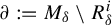
 absorbed in
$\partial := M_\delta \setminus R^i_\delta $
 . To do so, we adapt the analysis of conditionally invariant probability measures provided by Pianigiani and Yorke [Reference Pianigiani and Yorke65] as fixed points of the (normalized) Ruelle–Perron–Frobenius operator,
$\widehat {\mathcal {L}_\varepsilon }$
 . We continue with a detailed study of the operator
$\mathcal {P}_\varepsilon $
 to obtain the (unique) eigenfunction
$g_\varepsilon $
 of maximal eigenvalue
$\unicode{x3bb} _\varepsilon $
 . Finally, we prove the existence and uniqueness of a quasi-ergodic measure of the
$e^\phi $
 -weighted Markov process
$X_n^\varepsilon $
 conditioned upon not escaping the support of
$g_\varepsilon $
 , and characterize its limiting behaviour as the noise strength
$\varepsilon $
 vanishes. This measure follows from the pointwise product of
$\mu _\varepsilon $
 and
$g_\varepsilon $
 . As previously mentioned, we show that the limiting object as
$\varepsilon \to 0$
 corresponds to an ergodic invariant measure sitting on the repelling set
$R^i$
 that corresponds to the unique equilibrium state for the potential
$\phi -\log |\!\det d T |$
 .
Throughout this section, we assume Hypothesis H1 holds true and employ the notation introduced in §2. In particular, we use ‘
$\varepsilon $
 small enough’ and ‘
$\delta $
 small enough’ to refer to
$\varepsilon $
 and
$\delta $
 as in Lemmas 2.11, 3.1 and 3.2. All arguments in this section hold for each
$1 \leq i\leq k$
 and every
$\alpha $
 -Hölder weight function
$\phi :R^i_\delta \to \mathbb {R}$
 , which we fix once and for all. To improve readability, we drop the super-index
$\phi $
 of the weighted Markov process
$X_n^{\varepsilon ,\phi }$
 and simply write
$X_n^{\varepsilon }$
 .
4.1 Quasi-stationary measures on
$R_\delta ^i$

Denote by
$\widehat {\mathcal {L}_\varepsilon }$
 the
$L^{1}$
 -normalized operator
$\mathcal {L}_\varepsilon $
 , i.e.

Notation 4.1. Given a compact metric space
$(N,d)$
 and
$0<\alpha <1$
 , we denote by
${\mathcal {C}}^{\alpha }(N)$
 the set of
$\alpha $
 -Hölder functions
$f:N \to \mathbb {R}$
 and consider the
$\alpha $
 -Hölder norm

To obtain a quasi-stationary density for the conditioned process on each component
$R^{i}_\delta $
 , we apply the Schauder–Tychonoff fixed point theorem (see, e.g., [Reference Viana and Oliveira82, Theorem 2.2.3]) to the operator
$\widehat {\mathcal {L}_\varepsilon }$
 acting on a suitable space
$C_\beta $
 .
Theorem 4.2. Consider an
$\alpha $
 -Hölder weight function
$\phi :R^i_\delta \to \mathbb {R}$
 and suppose that T satisfies Hypothesis H1 on
$R^i$
 . Let
$\delta>0$
 be small enough. Then, for every
$\varepsilon>0$
 small enough, there exists a measure
$\mu _\varepsilon (dx)$
 on
$R^i_\delta $
 such that:
-
(1) $\mu _\varepsilon $
is a quasi-stationary measure of the
$e^\phi $
-weighted Markov process
$X_n^\varepsilon $
on
$R^i_\delta $
with growth rate given by
$\unicode{x3bb} _\varepsilon = r({\mathcal {L}}_\varepsilon :L^1(R_\delta ^i,\rho )\to L^1(R^i_\delta ,\rho )));$
-
(2) $\mu _\varepsilon $
is absolutely continuous with respect to
$\rho $
; and -
(3) defining $m_\varepsilon := \mu _\varepsilon (d x)/\rho (d x)$
, there exists
$C>0$
such that
$\|m_\varepsilon \|_{{\mathcal {C}}^\alpha }\leq C$
and
$m_\varepsilon (x)>0$
for every
$x\in R_\delta ^i.$


Proof. Given
$\beta>0$
 , consider the set

We divide the proof into three steps, first establishing the existence of the density
$m_\varepsilon \in C_\beta $
 .
Step 1. There exists
$\beta>0$
 such that
$\widehat {\mathcal {L}_\varepsilon } (C_\beta )\subset C_\beta. $

Proof of Step 1.
First of all, observe that if
$\delta>0$
 is small enough,
$f>0, f \in C_\beta ,$
 implies
${\mathcal {L}}_\varepsilon f>0$
 for every
$\varepsilon>0.$
 Define
$\psi : R_\delta ^i\to \mathbb R$
 as
$\psi := \phi - \log |\!\det \, d T|$
 and let

Recall from Lemma 3.2(3) that if
$\varepsilon>0$
 is small enough, then given
$x,y$
 in the same connected component C of
$R^i_\delta $
 , we have

for every
$\omega \in \Omega _\varepsilon .$
 Suppose that
$\#\{T^{-1}(x)\cap \Lambda _\delta \} = \ell .$
 Let
$h_1,\ldots ,h_\ell :[-\varepsilon ,\varepsilon ]^m\times C \to ~R_\delta ^i$
 be the pre-image functions (inverse branches) defined in Lemma 3.1. Given
$f\in C_\beta $
 , we have that

with
$\sigma $
 from Lemma 3.2. Therefore, if
$f\in C_\beta $
 , then
$ \widehat {\mathcal {L}_\varepsilon } f \in C_{\sigma ^\alpha (\beta +D)}.$
 Taking
$\beta> D \sigma ^\alpha /(1-\sigma ^\alpha )>0$
 , we conclude Step 1.
Step 2. For every
$\varepsilon>0$
 small, there exists
$m_\varepsilon \in C_\beta $
 such that
$\widehat {\mathcal {L}_\varepsilon }m_\varepsilon = m_\varepsilon .$

Proof of Step 2.
Observe that
$C_\beta $
 is pre-compact and convex in
$L^1(R_\delta ^i,\rho )$
 . From the Schauder fixed-point theorem, there exists
$m_\varepsilon $
 lying in the closure of
$C_\beta $
 such that
$\widehat {\mathcal {L}_\varepsilon }m_\varepsilon =~m_\varepsilon $
 , which implies that
${\mathcal {L}}_\varepsilon m_\varepsilon = \unicode{x3bb} _\varepsilon m_\varepsilon $
 for
$\unicode{x3bb} _\varepsilon = \|{\mathcal {L}}_\varepsilon m_\varepsilon \|>0.$
 We claim that
$m_\varepsilon \in C_\beta .$
 Suppose for a contradiction that
$m_\varepsilon \in \overline { C_\beta }^{{}_{L^1(R_\delta ^i,\rho )}}\setminus C_\beta .$
 Since
$m_\varepsilon \in \overline {C_\beta }^{{}_{L^1(R_\delta ^i,\rho )}}$
 , there exists a sequence
$m^{(n)}_\varepsilon \in C_\beta , n \in \mathbb N,$
 such that
$m^{(n)}_\varepsilon \xrightarrow []{n\to \infty }m_\varepsilon \ \text {in }L^1(R_\delta ^i,\rho ).$
 Moreover, from [Reference Salamon73, Corollary 4.10], there exists a subsequence
$\{m^{(n_k)}_\varepsilon \}_{k\in \mathbb N}\subset \{m^{(n)}_\varepsilon \}_{n\in \mathbb N}$
 such that
$m^{(n_k)}_\varepsilon \to m_\varepsilon $
 pointwise
$\rho $
 -almost surely. Therefore, for
$\rho $
 -a.e.
$x,y$
 lying in the same connected component of
$R_\delta ^i$
 ,

The above equation implies that we may choose a representative of
$m_\varepsilon $
 in
$L^1(R_\delta ,\rho )$
 that is continuous and, therefore, we obtain that the above equation holds for each
$x,y$
 lying in the same connected component of
$R_\delta ^i$
 . From (4.1) and
$m_\varepsilon \not \in C_\beta $
 , it must exist
$x\in R^i_\delta $
 such that
$m_\varepsilon (x) = 0.$
 It follows that
$m_\varepsilon (y) = 0$
 for every y in the same connected component
$C_x$
 of x in
$R^i_\delta $
 , as x and y may be interchanged in (4.1). Hence, for every
$y\in C_x$
 and
$n>0$
 ,

where
$S_n \phi (\omega ,z) = \sum _{i=0}^{n-1} \phi \circ T^i_\omega (z).$

This implies that
$m_\varepsilon $
 vanishes in the connected components of points in
$T^{-n}(y)\cap R_\delta ^i$
 for every
$y\in C_x$
 . Since there exists
$z\in R^i$
 such that
$\{T^n(z)\}_{n\in \mathbb N}$
 is dense in
$R^i$
 , it follows that
$m_\varepsilon \equiv 0$
 , which is a contradiction.
Step 3. We prove that if
$f\in L^1(R_\delta ^i, \rho )$
 , then
$ {\mathcal {L}}_\varepsilon f \in {\mathcal {C}}^0(R_\delta ^i)$
 .
Proof of Step 3.
Let
$x\in R_\delta ^i$
 and
$r>0$
 small enough. As in Step 1, let the function

be such that for each
$j\in \{1,\ldots , k\}$
 :
-
• $T_{\omega } \circ h_{j}(\omega ,z) = z$
for every
$(\omega _0,z)\in [-\varepsilon ,\varepsilon ]^m\times B_r(x)$
, for each
$i\in \{1,\ldots , k\}$
; -
• for any $z\in B_r(x)$
,
$T_\omega ^{-1}(z) = \{h_1(\omega ,x),\ldots , h_\ell (\omega ,x)\}.$


Moreover, since

we have that

which is well defined due to (3.1). Since
$\partial _\omega T_\omega $
 is full rank, we obtain that
$\partial _\omega h_j$
 is also full rank.
Given
$f\in L^1(R_\delta ^i,\rho )$
 , we have that defining
$\psi (\omega ,x) = \phi (x) - \log |\!\det d T_\omega (z)|$
 ,

Repeating verbatim the computations in the proof of Proposition 3.5, noting that this argument uses only the facts that the map F (which, in the present setting, is
$h_j$
 ) has full rank in the
$\omega $
 -variable and that
$f\in L^1(R_\delta ^i,\rho )$
 , we obtain the desired result.
We may now conclude the proof of the theorem.
Items (2) and (3) follow directly from Step 2. To prove item (1), define
$\mu _\varepsilon (d x) = m_\varepsilon (x)\,d x$
 , then for any
$f:R^i_\delta \to \mathbb {R}$
 bounded and measurable,

where
$\unicode{x3bb} _\varepsilon = \|{\mathcal {L}}_\varepsilon m_\varepsilon \|_1.$

From Step 3, we have that
${\mathcal {L}}_\varepsilon (L^1(R^i_\delta , \rho ) \subset {\mathcal {C}}^0(R^i_\delta ))$
 . Moreover,
${\mathcal {L}}_\varepsilon : L^1(R^i_\delta , \rho ) \to {\mathcal {C}}^0(R^i_\delta )$
 is a positive linear operator between Banach spaces; therefore,
${\mathcal {L}}_\varepsilon $
 is bounded (see [Reference Schaefer75, Theorem II.5.3], in particular, there exists
$K>0$
 ,

From Step 2, we have that
$\inf m_\varepsilon (x) = c>0$
 . Observe that for any
$f\in L^1(R^i_\delta , \rho ),$
 then for every
$x\in R_\delta ^i$
 ,

Therefore, using (4.2) and (4.3),

Since
$\unicode{x3bb} _\varepsilon \in \sigma ({\mathcal {L}}^1\to L^1)$
 , we have that
$\unicode{x3bb} _\varepsilon = r({\mathcal {L}}_\varepsilon )$
 , which implies item (1).
For the remainder of this section, let
$m_\varepsilon \in C_\beta $
 denote the unique function such that
$\mathcal {L}_\varepsilon m_\varepsilon = \unicode{x3bb} _\varepsilon m_\varepsilon $
 and let
$\mu _\varepsilon $
 be the unique quasi-stationary measure, i.e. be such that
$m_\varepsilon =~\mu _\varepsilon (dx)/\rho (dx)$
 , as in Theorem 4.2.
4.2 Analysis of the operator
$\mathcal {P}_\varepsilon :L^\infty (R_\delta ^i) \to L^\infty (R_\delta ^i)$

We now study the adjoint operator of
${\mathcal {L}}_\varepsilon $
 to obtain the eigenfunction
$g_\varepsilon $
 , associated with the maximal eigenvalue
$\unicode{x3bb} _\varepsilon $
 from the previous result, and its properties. We also construct the unique quasi-ergodic measure of the
$e^\phi $
 -weighted Markov process
$X_n^\varepsilon $
 on
$\{g_\varepsilon> 0\}$
 .
Lemma 4.3. Assume that T satisfies Hypothesis H1 on
$R^i$
 , let
$\delta , \epsilon> 0$
 be small enough and let
$\unicode{x3bb} _\varepsilon $
 be the eigenvalue associated with
$m_\varepsilon $
 from Theorem 4.2. Let
$g_\varepsilon \in \ker \, (\mathcal {P}_\varepsilon -\unicode{x3bb} _\varepsilon ) \cap {\mathcal {C}}^0_+(R^i_\delta )$
 , then
$R^i\subset \{g_\varepsilon>0\}$
 .
Proof. We divide the proof into two steps and note that the fact that
$\ker (\mathcal {P}_\varepsilon -\unicode{x3bb} _\varepsilon )\cap {\mathcal {C}}^0_+(R^i_\delta ) \neq \emptyset $
 will be shown in Theorem 4.4. First, we check that
$g_\varepsilon $
 is positive on dense orbits of T and, second, construct a neighbourhood of
$R^i$
 where
$g_\varepsilon $
 is positive. It is clear that a dense orbit exists since
$T:R^i \to R^i$
 is topologically transitive by Lemma 2.6. Let
$K_0 = \min _{x\in R_\delta ^i} e^{\phi (x)}>0.$

Step 1. If
$\{T^j (x_0)\}_{j\in \mathbb {N}}$
 is dense in
$R^i,$
 then
$g_\varepsilon (x_0)>0.$

Proof of Step 1.
Recall that
$g_\varepsilon \in {\mathcal {C}}_+^0(R_\delta ^i)$
 . Assume that
$g_\varepsilon (x_0) =0,$
 then for every
$n \in ~\mathbb {N}$
 ,

Combining this with the submersion theorem applied to
$\partial _\omega T_\omega $
 (see [Reference Lee59, Theorem 4.12]) and the fact that
$R_\delta ^i$
 is compact, we obtain that there exists
$r_0>0$
 such that
$g_\varepsilon |_{B_{r_0}(T^n(x_0))} =~0$
 for every
$n\in \mathbb {N}$
 . Since
$\{T^j(x_0)\}_{j \in \mathbb {N}}$
 is dense in
$R^i$
 , there exists a neighbourhood
$U\supset R^i$
 such that
$g_\varepsilon |_U = 0.$

Let
$T_{\cap R_\delta ^i}(U) := T(U \cap R_{\delta }^i)$
 . Recall that, from (3.2), there exists
$N\in \mathbb N$
 such that
$T^N_{\cap R_\delta ^i}(U) \supset R_\delta ^i$
 . Take
$y\in R_\delta ^i$
 . Then, there exists
$z\in U$
 such that
$T^N(z) = y$
 and
$T^j(z) \in U$
 for every
$j\in \{1,\ldots , N\}.$
 Since

continuity of
$g_\varepsilon $
 and the submersion theorem applied to
$\partial _\omega T_\omega $
 yields
$g_\varepsilon (y) = 0$
 . This contradicts
$g_\varepsilon \neq 0$
 .
Step 2. There exists an open set
$B\supset R^i$
 such that
$g_\varepsilon (x)>0$
 for every
$x\in B.$

Proof. Set
$B := \{x\in R_\delta ^i;\ \text { there exists }\ \omega _0 \in (-\varepsilon /2,\varepsilon /2)^m\ \text {such that }T_{\omega _0}(x)\in R^i\}.$
 From the submersion theorem, we have that given
$x\in B$
 and
$\omega _0 \in (-\varepsilon /2,\varepsilon /2)^m$
 such that
$T_{\omega _0}(x)\in R^i$
 , we obtain that there exists
$r_1>0$
 such that

Let
$x_0 \in R^i$
 be such that
$\{T^j(x_0)\}_{j\in \mathbb N}$
 is dense in
$R^i$
 , then there exists
$N_0$
 such that
$T^{N_0}(x_0) \in B_{r_1}(T_{\omega _0} (x)).$
 From Step 1,
$g_\varepsilon (T^{N_0}(x_0))>0.$
 Continuity of
$g_\varepsilon $
 then implies

This concludes Step 2.
The lemma is now proved.
Theorem 4.4. Consider the operator
$\mathcal {P}_\varepsilon :L^\infty (R^i_\delta ) \to L^\infty (R^i_\delta )$
 . Then,
$\ker (\mathcal {P}_\varepsilon - \unicode{x3bb} _\varepsilon )= \mathrm {span}(g_\varepsilon )$
 for some
$g_\varepsilon \in {\mathcal {C}}^0_+(R_\delta ^i).$

Proof. Let
$g_\varepsilon \in \ker (\mathcal {P}_\varepsilon -\unicode{x3bb} _\varepsilon )$
 . Since
$\mathcal {P}_\varepsilon $
 is strong Feller, then
$g_\varepsilon \in {\mathcal {C}}^0(R_\delta ^i,\mathbb C)$
 . Moreover, since
$\mathcal {P}_\varepsilon ({\mathcal {C}}^0(R_\delta ^i))\subset {\mathcal {C}}^0(R_\delta ^i),$
 it is clear that
$\mathrm {Re}(g_\varepsilon ),\mathrm {Im}(g_\varepsilon )\in \ker (\mathcal {P}_\varepsilon - \unicode{x3bb} _\varepsilon ).$
 Given
$g_\varepsilon \in \ker (\mathcal {P}_\varepsilon -\unicode{x3bb} _\varepsilon )\cap {\mathcal {C}}^0(R_\delta ^i)$
 , we claim that
$g^{\pm }_\varepsilon \in \ker (\mathcal {P}_\varepsilon -\unicode{x3bb} _\varepsilon ).$
 Indeed, observe that (see [Reference Lasota and Mackey58, Propositions 3.1.1 and 3.1.3])

where
$g_\varepsilon ^\pm = \max \{0, \pm g_\varepsilon \}. $
 Therefore,

From Theorem 4.2,
$\mathrm {supp}\, \mu _\varepsilon = R_\delta ^i;$
 therefore,
$\mathcal {P}_\varepsilon g_\varepsilon ^\pm = \unicode{x3bb} _\varepsilon g_\varepsilon ^\pm .$

Take
$g_1,g_2 \in \ker (\mathcal {P}_\varepsilon - \unicode{x3bb} _\varepsilon )\cap {\mathcal {C}}_+^0( R^i_\delta ).$
 From Lemma 4.3, we have
$g_1, g_2> 0$
 on
$R^i$
 . Choose
$t_0>0$
 such that
$t_0 =\inf \{t;\, g_1(x) - tg_2(x)<0\text { for some }x\in R^i\}.$

Since
$g_1 - t_0 g_2 \in \ker (\mathcal {P}_\varepsilon - \unicode{x3bb} _\varepsilon )$
 , then
$(g_1 - t_0g_2)^+ \in \ker (\mathcal {P}_\varepsilon - \unicode{x3bb} _\varepsilon ).$
 However, from the choice of
$t_0$
 and Lemma 4.3, we obtain that
$(g_1 - t_0g_2)^+=0$
 . From the minimality of
$t_0$
 , it follows that
$g_1(x) = t_0 g_2 (x)$
 for every
$x\in R^i.$
 Observe that
$(g_1 - t_0g_2)^+=0$
 yields that
$t_0 g_2 \geq g_1.$
 Therefore,
$t_0 g_2 -g_1 \in \ker (\mathcal {P}_\varepsilon - \unicode{x3bb} _\varepsilon )\cap {\mathcal {C}}^0_+(R^i_\delta )$
 and
$(t_0 g_2 -g_1)|_{R^i}=~0,$
 which implies that
$t_0 g_2 -g_1 = 0$
 .
Theorem 4.5. There exists a unique quasi-stationary measure
$\mu $
 on
$R_\delta ^i$
 for
$X^\varepsilon _n$
 such that
$\Lambda \subset \mathrm {supp}\, \mu .$
 In fact, this quasi-stationary measure is the fully supported measure constructed in Theorem 4.2.
Proof. Let
$\mu $
 be a quasi-stationary measure on
$R_\delta ^i$
 with growth rate
$\unicode{x3bb} $
 . We divide the proof into two cases: (i)
$\unicode{x3bb} \neq \unicode{x3bb} _\varepsilon $
 and (ii)
$\unicode{x3bb} = \unicode{x3bb} _\varepsilon $
 .
To prove the result in case (i), observe that
$g_\varepsilon \in \mathrm {ker}({\mathcal {P}}_\varepsilon -\unicode{x3bb} _\varepsilon ) \cap {\mathcal {C}}^0_+(R_i^\delta )$
 and
$\{g_\varepsilon>~0\} \supset \Lambda $
 , from Lemma 4.3 and Theorem 4.4. It follows that

Since
$\unicode{x3bb} \neq \unicode{x3bb} _\varepsilon $
 , we obtain that
$\int _{R_\delta ^i} g_\varepsilon (x) \mu (d x) =0$
 , which implies that
$\mathrm {supp}\, \mu \cap \Lambda = \emptyset .$

To prove the result in case (ii), since
${\mathcal {P}}_\varepsilon (x,d y) \ll \rho (d y)$
 for every
$x\in R_\delta ^i$
 (recall Lemma A.2), we have that
$\mu \ll \rho $
 . Define

Since
$\mu (d x) = m (x)\,d x$
 , we have that
${\mathcal {L}}_\varepsilon m = \unicode{x3bb} _\varepsilon m$
 ; however,
$\unicode{x3bb} _\varepsilon $
 is a simple eigenvalue of
${\mathcal {L}}_\varepsilon $
 , which follows from the fact that
${\mathcal {L}}_\varepsilon ^* = {\mathcal {P}}_\varepsilon $
 ,
${\mathcal {P}}_\varepsilon $
 is a quasi-compact operator (since
${\mathcal {P}}_\varepsilon ^2$
 is compact, see Lemma A.2 in Appendix A) and
$\unicode{x3bb} _\varepsilon = r({\mathcal {P}}_\varepsilon )$
 is a simple eigenvalue (see Theorem 4.4).
For the remainder of this section, let
$g_\varepsilon \in {\mathcal {C}}^0_+(R^i_\delta )$
 denote the unique function such that
$\mathcal {P}_\varepsilon g_\varepsilon = \unicode{x3bb} _\varepsilon g_\varepsilon $
 and normalized so that
$\int g_\varepsilon d\mu _\varepsilon = 1$
 , as in Theorems 4.4 and 4.5. We summarize some relevant properties of
$\mathcal {P}_\varepsilon :L^\infty (R_\delta ^i) \to L^\infty (R^i_\delta )$
 that have been shown above:
-
(1) $\mathcal {P}_\varepsilon : L^\infty (R_\delta ^i,\rho )\to L^\infty (R_\delta ^i,\rho )$
is a strong Feller operator; -
(2) $\dim \ker (\mathcal {P}_\varepsilon - \unicode{x3bb} _\varepsilon ) =1$
, where
$\unicode{x3bb} _\varepsilon = r(\mathcal {P}_\varepsilon )$
is the spectral radius; -
(3) there exists $\mu _\varepsilon \in {\mathcal {M}}_+(R_\delta ^i)$
and
$g_\varepsilon \in {\mathcal {C}}^0_+(R_\delta ^i)$
such that
$\mathcal {P}^*_\varepsilon \mu _\varepsilon = \unicode{x3bb} _\varepsilon \mu _\varepsilon $
and
$\mathcal {P}_\varepsilon g_\varepsilon = \unicode{x3bb} _\varepsilon g_\varepsilon $
; -
(4) $\mu _\varepsilon \ll \rho $
and
$\text {{supp}}\, \mu _\varepsilon = R_\delta ^i$
; and -
(5) $\mu _\varepsilon $
is the unique quasi-stationary measure of
$X_n^\varepsilon $
on
$R_\delta ^i$
such that
$\Lambda \subset \mathrm {supp}\, \mu _\varepsilon $
.


In particular, this implies that
$\mathcal {P}_\varepsilon $
 satisfies Hypothesis HA in Appendix A. The lemma below is a consequence of the properties just listed and Theorems A.13 and A.14, whose proof is deferred to the Appendix in order not to break the flow of the text.
Lemma 4.6. The measure
$\nu _\varepsilon (d x) := g_\varepsilon (x) \mu _\varepsilon (d x)$
 is the unique quasi-ergodic measure of the
$e^\phi $
 -weighted Markov process
$X_n^\varepsilon $
 on
$\{g_\varepsilon>0\}$
 . If we further assume that
$T:R^i\to R^i$
 is topologically mixing, then
$\nu _\varepsilon $
 is also a quasi-ergodic measure of the
$e^\phi $
 -weighted Markov process
$X_n^\varepsilon $
 on
$R^{i}_\delta $
 .
Proof. It is clear from the properties of
$\mathcal {P}_\varepsilon $
 listed above that it satisfies Hypothesis HA (see Appendix A). Hence, Theorem A.13 implies that
$\nu _\varepsilon $
 is the unique
$e^\phi $
 -weighted quasi-ergodic measure for
$X_n^\varepsilon $
 on
$\{g_\varepsilon>0\}$
 .
To finish the proof of the theorem, it remains to be shown that if T is topologically mixing, then
$\nu _\varepsilon $
 is an
$e^\phi $
 -weighted quasi-ergodic measure for
$X_n^\varepsilon $
 on
$R^i_\delta $
 . Since T is topologically mixing, then
$X_n^\varepsilon $
 is aperiodic in
$R^i_\delta $
 and
$\{g_\varepsilon>0\}$
 . Let
$k_\varepsilon := \#(\sigma _{\mathrm {per}}(({1}/{\unicode{x3bb} _\varepsilon }){\mathcal {P}}_\varepsilon )\cap \mathbb S^1 )$
 . From Lemma A.3,
$k_\varepsilon <\infty $
 . Moreover, from Proposition A.6 and Lemma A.7, we obtain that there exist sets
$C_i \subset \{g_\varepsilon>0\}$
 ,
$i\in \{0,1,\ldots ,k_\varepsilon -1\}$
 such that
$C_0 \sqcup C_1 \sqcup \cdots \sqcup C_{k_\varepsilon -1} = \{g_\varepsilon>0\},$
 and
$\{{\mathcal {P}}_\varepsilon \mathbb {1}_{C_i}>0 \}\subset C_{i-1\ (\mathrm {mod}\ k_\varepsilon )}$
 for every
$i\in \{0,1,\ldots ,k_\varepsilon ~-1\}$
 . Since T is assumed to be topologically mixing on
$R^i$
 ,
$X_n^\varepsilon $
 is aperiodic and, thus,
$k_\varepsilon =1$
 . Finally, from Theorem A.14, we obtain that
$\nu _\varepsilon $
 is a quasi-ergodic measure of the
$e^\phi $
 -weighted Markov process
$X_n^\varepsilon $
 on
$R^i_\delta $
 .
4.3 The limit
$\varepsilon \to 0$
. Proof of the main (local) result

We conclude this section with the main results concerning the stochastic stability of equilibrium states on each repeller
$R^i_\delta $
 and their limiting behaviour as
$\varepsilon \to 0$
 .
Notation 4.7. Recall that given a suitable function f, we denote the action of the (deterministic) Ruelle–Perron–Frobenius operator
$\mathcal {L}$
 for the potential
$\psi = \phi -\log |\!\det d T|$
 [Reference Viana and Oliveira82, Ch. 12] by (observe that the potential in Theorem 2.7 is simply
$\phi $
 )

when this is well posed (see Theorem 2.7). In particular, this is the case for any function supported on
$R_\delta ^i$
 .
Lemma 4.8. Consider a sequence
$\{m_\varepsilon \}_{\varepsilon>0} \subset {\mathcal {C}}^\alpha (R_\delta ^i)$
 , with
$\|m_\varepsilon \|_{{\mathcal {C}}^\alpha } \leq C$
 for every
$\varepsilon> 0$
 . Then,
${\|\mathcal {L}_\varepsilon m_\varepsilon - \mathcal {L} m_\varepsilon \|_{L^\infty } \xrightarrow []{\varepsilon \to 0} 0.}$

Proof. Using the usual bounds, we have that

where
$N = \sup _{(x,\omega ) \in R_\delta ^i\times \Omega _\varepsilon }\# (T_\omega ^{-1}(\{x\}\cap R_\delta ^i)<\infty $
 , the
$K_i$
 provide a bound for the term
$|\!\det d T_\omega (h_i(\omega , x))^{-1}|$
 ,
$C\sup |D_\omega h_i|^\alpha \varepsilon ^\alpha $
 are a Hölder-like bound for the difference

and so is
$K_i' \sup |D_\omega h_i| \varepsilon $
 for
$({|\!\det d T_\omega (h_i(\omega , x))|}^{-1} -{|\!\det d T(h_i(0, x))|}^{-1}|)^{-1}$
 .
Proposition 4.9. Let
$m_\varepsilon :R_\delta ^i\to \mathbb R$
 be the functions given by Theorem 4.2. There exist
$\unicode{x3bb} _0>0$
 and
$m_0\in {\mathcal {C}}^0(R_\delta ^i)$
 such that
$\unicode{x3bb} _\varepsilon \xrightarrow []{\varepsilon \to 0}\unicode{x3bb} _0$
 and
$m_\varepsilon |_{R^i} \xrightarrow []{\varepsilon \to 0} m_0$
 in
${\mathcal {C}}^0(R^i)$
 , with
${\mathcal {L}} m_0 = \unicode{x3bb} _0 m_0$
 .
Proof. Since
$\|m_\varepsilon \|_{{\mathcal {C}}^\alpha }\leq C,$
 there exists
$\{\varepsilon _n\}_{n\in \mathbb N}$
 such that
$\varepsilon _n \to 0$
 and
$m_0\in {\mathcal {C}}^0(R_\delta ^i)$
 , such that
$\|m_{\varepsilon _n} - m_0\|_{{\mathcal {C}}^0(R_\delta ^i)} \to 0.$
 We can assume without loss of generality, by restricting to a subsequence if necessary, that
$\unicode{x3bb} _{\varepsilon _n} \to \unicode{x3bb} _0 \geq 0,$
 which can be done since
$\unicode{x3bb} _\varepsilon \leq \|{\mathcal {L}}_\varepsilon \|_{{\mathcal {C}}^\alpha }$
 and the latter is uniformly bounded for
$0<\varepsilon <\varepsilon _0$
 . From Lemma 4.8, we obtain that

In the following, we show that
$\unicode{x3bb} _0>0$
 . Since
$\int _{R^i_\delta } m_{\varepsilon _n}(x)\rho (d x) = 1$
 for every
$n\in \mathbb N$
 , then by the Lebesgue-dominated convergence theorem,
$\int _{R^i_\delta }m_0(x)\rho (d x) =1$
 . Therefore, there exists
$x_0\in R^i_\delta $
 such that
$m_0(x_0)>0.$
 Let
$C_{x_0}\subset R^i_\delta $
 be the connect component of
$x_0$
 in
$R^i_\delta $
 . From the proof of Theorem 4.2 (Step 2), we obtain that for every
$n\in \mathbb N$
 ,
$e^{- \beta d(x_0,y) }m_{\varepsilon _{n}}(x_0) \leq m_{\varepsilon _{n}}(y)$
 for every
$y\in C_{x_0}$
 . Therefore, taking
$n\to \infty $
 , we obtain that
$0 < m_0(y)$
 for every
$y\in C_{x_0}.$
 In particular,
$m_0|_{R^i} \neq 0.$
 Assume for a contradiction that
$\unicode{x3bb} _0=0$
 . Then, for every
$x\in R^i$
 ,

Since
$R^i \subset T^{-1}(R^i)$
 , the above equation implies that
$m_0|_{R^i} =0$
 , which is a contradiction. Therefore,
$\unicode{x3bb} _0>0$
 .
Since there exists a unique
$m_0 \in {\mathcal {C}}^0(R^i)$
 such that
$\mathcal {L} m_0(x) = \unicode{x3bb} _0 m_0(x)$
 for every
$x\in R^i$
 and
$\unicode{x3bb} _0>0$
 [Reference Viana and Oliveira82, Ch. 12], the proposition follows.
Proposition 4.10. Let
$g_\varepsilon \in {\mathcal {C}}^0_+(R_\delta ^i)$
 be the functions given by Theorem 4.4 and consider
$\unicode{x3bb} _0>0$
 as in Proposition 4.9. There exists a probability measure
$\gamma $
 on
$R^i_\delta $
 such that
${g_{\varepsilon }(x)\,dx \xrightarrow {\varepsilon \to 0}\gamma (d x)}$
 in the weak
$^*$
 topology of
${\mathcal {M}}(R_\delta ^i)$
 . Moreover,
$\gamma $
 is the unique conformal measure for T on
$R^i$
 for the potential
$\phi -\log |\!\det d T|$
 , i.e.
$\gamma $
 is the unique probability measure on
$R^i$
 such that
${\mathcal {L}}^* \gamma = \unicode{x3bb} _0 \gamma $
 .
Proof. Let
$\gamma $
 be an accumulation point of
$\{g_\varepsilon (x)\,d x\}_{\varepsilon>0}$
 in the weak
$^*$
 topology of
${\mathcal {M}}(R_\delta ^i)$
 , i.e. there exists a sequence
$\{g_{\varepsilon _n}(x)\,d x\}_{n\in \mathbb {N}}$
 such that
$\varepsilon _n \xrightarrow []{n\to \infty }0$
 and
${g_{\varepsilon _n}(x)\,dx \xrightarrow []{n\to \infty }\gamma (d x)}$
 in the weak
$^*$
 topology. We first check that
$\gamma $
 is a conformal measure on
$R_\delta ^i$
 . Indeed, for a test function
$f \in {\mathcal {C}}^\alpha (R^i_\delta )$
 , we have

We claim that
${\mathrm {supp}}\, \gamma \subset R^i$
 . From item (2) in Lemma 2.11 and items (1) and (2) in Lemma 3.2, we obtain that

Repeating this argument n times, we obtain that
$\gamma (R_{\sigma _0^n \delta }^i) = 1$
 and the claim follows by taking
$n\to \infty $
 . Since there exists a unique measure
$\gamma $
 in
$R^i$
 such that
$\mathcal {L}^* \gamma = \unicode{x3bb} _0 \gamma $
 (see [Reference Viana and Oliveira82, Ch. 12]), we conclude that
$g_\varepsilon (x)\,d x \xrightarrow {\varepsilon \to 0} \gamma (d x)$
 in the weak
$^*$
 topology.
Proposition 4.11. Assume that T satisfies Hypothesis H1 on
$R^i$
 . Let
$\nu _\varepsilon $
 be the unique quasi-ergodic measure of the
$e^\phi $
 -weighted Markov process
$X_n^\varepsilon $
 on
$\{g_\varepsilon>0\}$
 . Then,
$\nu _\varepsilon \xrightarrow []{\varepsilon \to 0}\nu _0(x) := m_0(x) \gamma (d x),$
 in the weak
${}^*$
 topology. Moreover,
$\nu _0$
 is the unique T-invariant equilibrium state for the potential
$\phi -\log |\!\det d T|$
 in
$R^i$
 .
Proof. From Lemma 4.6, we have that
$\nu _\varepsilon (d x) = g_\varepsilon (x) \mu _\varepsilon (d x)$
 is the unique quasi-ergodic measure of the
$e^\phi $
 -weighted Markov process
$X_n^\varepsilon $
 on
$\{g_\varepsilon>0\}$
 such that
$R^i\subset \mathrm {supp}\, g_\varepsilon $
 . Since
$m_\varepsilon \xrightarrow []{\varepsilon \to 0} m_0$
 in
${\mathcal {C}}^0(R_\delta ^i)$
 and
$g_\varepsilon (x)\,d x \xrightarrow []{\varepsilon \to 0} \gamma (d x)$
 in the weak
$^*$
 topology, then
$\nu _\varepsilon \xrightarrow []{\varepsilon \to 0}\nu _0$
 in the weak
$^*$
 topology. The final part of the proposition follows from well-known results in the thermodynamic formalism for expanding maps (see [Reference Viana and Oliveira82, Ch. 12]).
We close this section proving Theorem 2.12.
Proof of Theorem 2.12.
Item (1) follows from Theorems 4.2 and 4.5, item (2) follows from Theorem 4.5 and Proposition 4.9, item (3) follows from Theorem 4.4, item (4) follows from Lemma 4.6, and items (5) and (6) follow from Proposition 4.11. Thus, only the last statement is left to check.
If
$\nu _0^\phi $
 is mixing for the map
$T:R^i\to R^i$
 , then
$T:R^i\to R^i$
 is topologically mixing since
$\mathrm {supp}\, \nu _0^\phi = R^i$
 . From Lemma 4.6, we obtain that
$\nu _\varepsilon ^\phi $
 is a quasi-ergodic measure of the
$e^\phi $
 -weighted Markov process
$X_\varepsilon ^\phi $
 on
$R^i_\delta $
 and the result follows.
Corollary 4.12. Assume Hypothesis H1 and that
$T|_{R^i}$
 is topologically mixing. Let
$\delta>0$
 be small enough. For every
$\varepsilon>0$
 sufficiently small, let
$\nu _\varepsilon (d x)$
 be the unique quasi-ergodic measure of the
$e^\phi $
 -weighted Markov process
$X_n^\varepsilon $
 on
$R^i_\delta $
 such that
$R^i \subset \mathrm {supp}\, \nu _\varepsilon $
 . Then,
$\nu _\varepsilon (d x) \xrightarrow []{\varepsilon \to 0}\nu _0(d x)$
 in the weak
$^*$
 topology. Finally,
$\nu _0$
 is the unique T-invariant equilibrium state for the potential
$\phi -\log |\!\det d T|$
 on
$R^i$
 .


5 The global problem
We will prove conditioned stochastic stability of equilibrium states on the global repeller
$\Lambda $
 by studying the quasi-ergodic measure of the
$e^\phi $
 -weighted Markov process
$X_n^\varepsilon $
 on
$\Lambda _\delta $
 and absorbed in
$\partial := U \cup (E \setminus M_\delta )$
 for some open set
$U\subset M$
 . As in §4, let us fix once and for all an
$\alpha $
 -Hölder weight function
$\phi : M_\delta \setminus U \to \mathbb {R}$
 . Moreover, we assume that
$(T,\phi ,\Lambda )$
 satisfies Hypothesis H2, with
$\Lambda $
 as in (1.1).
We start by arguing that restricting the study of quasi-ergodic measures on
$\Lambda _\delta $
 is sufficient to characterize those on
$M_\delta \setminus U$
 . Then, we decompose
$\Lambda _\delta $
 into transient and recurrent subsets, the latter being those that contain the original repellers
$R^i$
 . In particular, we show that all the relevant information for the global dynamics follows from the recurrent subset containing the repeller
$R^0$
 of maximal growth rate. The stochastic stability of global equilibrium states is then inferred via the stochastic stability of equilibrium states around
$R^0$
 .
Proposition 5.1. Assume that
$(T,\phi ,\Lambda )$
 satisfies Hypothesis H2. Let
$\delta>0$
 be sufficiently small and
$\mu _\varepsilon $
 be a quasi-stationary measure of the
$e^\phi $
 -weighted Markov process
$X_n^\varepsilon $
 on
$M_\delta \setminus U$
 . Then, for sufficiently small
$\varepsilon>0$
 :
-
(1) $\mu _\varepsilon \ll \rho ;$
-
(2) $\mathrm {supp}\, \mu _\varepsilon \cap \Lambda _\delta \neq \emptyset $
; and -
(3) $\mu _\varepsilon |_{\Lambda _\delta },$
after normalization, is a quasi-stationary measure of the
$e^\phi $
-weighted Markov process
$X_n^\varepsilon $
on
$\Lambda _\delta $
.


Proof. Observe that item (1) follows directly from the fact that
$\mathcal {P}_\varepsilon (x,d y) \ll \rho (d y)$
 for every
$x\in M_\delta \setminus U$
 .
To show item (2), arguing for a contradiction, suppose that
$\mathrm {supp}\,\mu _\varepsilon \cap \Lambda _\delta = \emptyset $
 . We claim that there exists
$N \in \mathbb {N}$
 and
$\varepsilon>0$
 small enough such that for every
$x\in \overline {M_\delta \setminus \Lambda _\delta }$
 , there exists
$i\in \{0,1,\ldots , N\}$
 such that
$T^i_\omega (x) \in U\cup (E\setminus M_\delta )$
 for every
$\omega \in \Omega _\varepsilon $
 , or in other words,
$\tau (x,\omega ) \leq N$
 for every
$\omega \in \Omega _\varepsilon $
 . This is sufficient to prove item (2) since, if true, any measurable set
$A \subset M_\delta \setminus U$
 would be assigned measure zero:

which is a contradiction. To verify the claim, choose
$y \in \overline {M_\delta \setminus \Lambda _\delta }$
 . Then, there exists
$n(y) \in \mathbb N$
 such that
$T^n(y) \in U \cup (E \setminus M_\delta )$
 . Since this is an open set, by continuity of T and
${\mathcal {C}}^2$
 closeness of the perturbation, there exists
$r(y)> 0$
 and
$\varepsilon (y)>0$
 such that
$T^{n(y)}_\omega (B_{r(y)}(y)) \subset U \cup (E \setminus M_\delta )$
 for all
$\omega \in \Omega _{\varepsilon (y)}$
 . Consider a finite open cover of
$M_\delta \setminus ~\Lambda _\delta $
 with such balls around n points
$y_1, \ldots , y_n$
 with respective radius
$r(y_1), \ldots , r(y_n)$
 . Setting
$N = \max \{n(y_1), \ldots , n(y_n)\}$
 and
$\varepsilon = \min \{\varepsilon (y_1),\ldots ,\varepsilon (y_n)\}$
 , the claim follows.
Finally, we show item (3). Since
$T^{-1}(\Lambda )\cap M = \Lambda ,$
 from the same proof of Lemma 3.2(2) and (3), we obtain that
$T_\omega ^{-1}(\Lambda _\delta ) \cap M_\delta \subset \Lambda _\delta $
 for every
$\omega \in \Omega _\varepsilon $
 . Let A be a measurable subset of
$\Lambda _\delta $
 , then

so
$\mu _\varepsilon |_{\Lambda _\delta }$
 normalized is a quasi-stationary measure of the
$e^\phi $
 -weighted Markov process
$X_\varepsilon ^\phi $
 on
$\Lambda _\delta $
 .
Proposition 5.2. Assume that
$(T,\phi ,\Lambda )$
 satisfies Hypothesis H2. Consider the operator
$\mathcal {P}_\varepsilon : L^\infty (M_\delta \setminus U) \to L^\infty (M_\delta \setminus U) $
 . If
${g \in L_+^\infty (M_\delta \setminus U)}$
 is such that
$\mathcal {P}_\varepsilon g = \unicode{x3bb} _\varepsilon g$
 , then
$g |_{M_\delta \setminus \Lambda _\delta }=0$
 .
Proof. The proof of Proposition 5.1 yields that for
$\varepsilon>0$
 small enough, there exists N such that
$T_\omega ^N(x) \in U$
 for every
$x \in M_\delta \setminus \Lambda _\delta $
 and
$\omega \in \Omega _\varepsilon $
 . Therefore,

It follows that for every
$x\in M_\delta \setminus \Lambda _\delta $
 and
$N> 0$
 ,

verifying the claim.
As a result of Propositions 5.1 and 5.2, it is natural to redefine the operator
$\mathcal {P}_\varepsilon $
 as

and denote by
$\unicode{x3bb} _\varepsilon = r(\mathcal {P}_\varepsilon )$
 its spectral radius. Moreover, observe that

is well defined and that
${\mathcal {L}}_\varepsilon ^* = \mathcal {P}_\varepsilon .$

5.1 Recurrent and transient regions
In this section, we represent the relevant dynamical behaviour of the absorbing Markov process
$X_n^\varepsilon $
 for every
$\varepsilon> 0$
 via a graph whose vertices are the connected components of
$\Lambda _\delta $
 . This approach resembles the graphs constructed via chain recurrence and filtration methods for classical dynamical systems (see [Reference Crovisier and Potrie30, Reference De Leo and Yorke33, Reference De Leo and Yorke34]). Later, we use this construction to characterize the support of the relevant quasi-stationary measure of the
$e^\phi $
 -weighted Markov process
$X_n^\varepsilon $
 .
Given
$\varepsilon>0,$
 we define an equivalence relation
$\sim _\varepsilon $
 on the set of connected components

as follows. For any
$C_1,C_2\in \Gamma _\delta $
 , we say that
$C_1\sim _{\varepsilon } C_2$
 if:
-
• $C_1=C_2$
; or -
• both sets are reachable from each other, i.e. for every $i,j\in \{1,2\}$
, there exist sets
$W_0, W_1,\ldots , W_n, W_{n+1} \in \Gamma _\delta $
such that
$\min _{\ell \in \{0,\ldots ,n\}}\sup _{x\in W_\ell }\mathcal {P}_\varepsilon (x, W_{\ell +1})>0, $
with
$W_0 = C_i$
and
$W_{n+1} = C_j$
.


Proposition 5.3. Assume that
$(T,\phi ,\Lambda )$
 satisfies Hypothesis H2. The set of equivalence classes
$\Gamma _\delta /\sim _\varepsilon $
 stabilizes as
$\varepsilon \to 0,$
 i.e. there exist
$C_1,\ldots ,C_n \in \Gamma _\delta $
 such that for every
$\varepsilon $
 small enough, we have that

where
$[C_i]$
 represents the equivalence class of the element
$C_i.$

Proof. The cardinality of
$\Gamma _\delta $
 is finite and observe that if
$0<\varepsilon _1<\varepsilon _2$
 , then
$C_1 \sim _{\varepsilon _1} C_2$
 implies
$C_1 \sim _{\varepsilon _2} C_2$
 . This ensures that
$\Gamma _\delta /\sim _\varepsilon $
 stabilizes as
$\varepsilon \to 0.$

Definition 5.4. Given
$\delta>0$
 small enough, let
$C_1,\ldots ,C_n \in \Gamma _\delta $
 be the sets given in Proposition 5.3. Define

i.e.
$M_i$
 is the (disconnected) region spanned by all elements in the class
$[C_i]$
 . Then, we have the following conditions.
-
• If there exists $j \in \{1, \ldots , k\}$
such that
$R^j_\delta \subset M_i$
, we say that
$M_i$
is a recurrent region. -
• If there are no sets $R_\delta ^j$
intersecting
$M_i$
, we say that
$M_i$
is a transient region.


Lemma 5.5. All regions
$M_i$
 can be classified as either recurrent or transient.
Proof. Assume that
$M_i$
 is not a transient region so that there exists
$R^j_\delta $
 such that
$R_\delta ^j \cap M_i \neq \emptyset $
 . Then, there exists a connected component
$C \Subset R^j_{\delta }$
 such that
$C \subset M_i$
 . Since T is topologically transitive on
$R^j$
 , we obtain that
$R^j_\delta \subset M_i$
 and, therefore,
$M_i$
 is recurrent.
Proposition 5.6. Let
$M_t$
 be a transient region. Then, there exists
$N \in \mathbb {N}$
 such that for all
$x \in M_t$
 ,
$\mathcal {P}^n_\varepsilon (x, M_t) = 0 \text { for all } n \geq N.$

Proof. We begin by showing that there exists
$N\in \mathbb {N}$
 such that for every
$x\in M_t$
 , either:
-
• $T^n(x) \in \mathrm {Int}(\bigcup M_{r})$
for some
$n \leq N$
, where
$\bigcup M_{r}$
is the union of all recurrent regions; or -
• $T^n(x) \not \in \Lambda _\delta $
for some
$n \leq N$
.


Let
$x\in \widetilde {\Lambda } \cap M_t,$
 where

There exists an open neighbourhood
$U_x$
 of x such that
$T^{n_x}(U_x) \subset \mathrm {Int}( \bigcup M_{r} )$
 , the union of recurrent regions. Since
$\widetilde \Lambda \cap M_t$
 is compact, there exist points
$x_1,\ldots , x_{s}$
 with respective open neighbourhoods
$U_{x_1}, \ldots , U_{x_s}$
 such that

Set
$N = \max \{n_{x_1},\ldots , n_{x_s}\}.$

However, observe that for every
$y\in M_t\setminus \widetilde \Lambda \subset M_\delta \setminus \widetilde \Lambda $
 , it follows from T satisfying Hypothesis H2 and [Reference Viana and Oliveira82, Theorem 11.2.14] that there exists
$n_y$
 such that
$T^{n_y}(y) \notin \Lambda _\delta .$
 From continuity, there exists an open neighbourhood
$V_y$
 of y such that
$T^{n_y}(V_y)\cap \Lambda _\delta =\emptyset .$
 Since
$M_t\setminus B$
 is compact, there exist
$y_1,\ldots , y_{m}$
 with respective open neighbourhoods
$V_{y_1}, \ldots , V_{y_m}$
 such that

Set
$N = \max \{n_{y_1},\ldots ,n_{y_m}\}.$
 From continuity of
$(x,\omega )\to T_\omega (x)$
 , we obtain that for every
$x\in M_t$
 , either
$T^n_\omega (x) \in \bigcup M_{r}$
 for every
$\omega \in \Omega _\varepsilon $
 and some
$n \leq N$
 ; or
$T^n_\omega (x) \notin \Lambda _\delta $
 for every
$\omega \in \Omega _\varepsilon $
 and some
$n \leq N$
 . In the first case, allowing return to
$M_t$
 would join the equivalence classes
$[C_t]$
 of
$M_t$
 with
$[C_r]$
 for some recurrent region
$M_r$
 , contradicting transience. In the second case, once the process escapes
$\Lambda _\delta $
 , it is killed. Thus,
${\mathcal {P}}_\varepsilon ^n(x,M_t) =~0$
 for every
$n>N$
 .
Proposition 5.6 naturally motivates the following definition.
Definition 5.7. Fix
$\varepsilon>0$
 such that the conclusions of Proposition 5.3 hold. Let
$M_1,\ldots , M_n$
 be the sets introduced in Definition 5.4. We define the directed graph
$\mathscr {G}_\delta =( V_\delta , E)$
 in the following way:
-
• the set of vertices $V_\delta $
is given by
$V_\delta := \{M_1,\ldots , M_n\}$
; -
• given $M_i,M_j\in V_\delta $
, we say that the edge
$M_i \to M_j$
is in
$E_\varepsilon $
if
$M_i\neq M_j$
and there exists
$x\in M_{i}$
such that
${\mathcal {P}}_\varepsilon (x,M_j)>0.$


Observe that using the same argument as in Proposition 5.3, the set of edges E does not depend on
$\varepsilon $
 as long as this parameter is small enough.
Proposition 5.8. Given a transient region
$M_t\in V_\delta $
 , there exists a path in
$\mathscr G_\delta $
 connecting
$M_t$
 to a recurrent region
$M_r$
 . Moreover, the graph
$\mathscr G_\delta $
 is acyclic.
Proof. To see the first part of the proposition, observe that there exists
$x\in M_{t}\cap (\Lambda \setminus R)$
 . In this way, there exists
$n\in \mathbb N$
 such that
$T^n(x) \in R.$
 Defining
$M_r$
 as the unique recurrent region such that
$T^n(x)\in M_r$
 , we obtain that there exists a path from
$M_t$
 to
$M_r$
 in the graph
$\mathscr G_\delta $
 .
Finally, observe that if
$\mathscr G_\delta $
 had a cycle, then this would contradict the maximality of the equivalence classes
$[C_1],\ldots , [C_n]$
 .
5.2 Proof of the main (global) result
Recall from Lemma 2.6 that
$R = \bigsqcup _{i=1}^{k}R^i$
 . For every
$i\in \{1,\ldots ,k\}$
 , consider the (deterministic) operator

and set
$\unicode{x3bb} _i = r(\mathcal {L}_i).$

Notation 5.9. Assume Hypothesis H2. Given a closed set
$A\subset \Lambda _\delta $
 , we write:
-
• $\mathcal {P}_{A,\varepsilon }: L^\infty (A,\rho ) \to L^\infty (A,\rho )$
,
$\mathcal {P}_{A,\varepsilon } f = \mathcal {P}_\varepsilon (\mathbb {1}_A \cdot f)$
; -
• $\mathcal {L}_{A,\varepsilon }: L^1(A,\rho ) \to L^1(A,\rho )$
,
$\mathcal {L}_{A,\varepsilon } f =\mathcal {L}_\varepsilon (\mathbb {1}_A \cdot f);$
and -
• for each vertex $M_v$
of the graph
$\mathscr G_\delta $
, we define $$ \begin{align*} \mathcal{L}_{M_v}: {\mathcal{C}}^0(M_v) &\to {\mathcal{C}}^0(M_v) \\* f &\mapsto \sum_{T(y)=x}\frac{e^{\phi(y) }f(y)\mathbb{1}_{M_v}(y)}{|\!\det d T(x) |}. \end{align*} $$
Note from Lemma 3.2 that this linear operator is well defined.


Lemma 5.10. Given a recurrent region
$M_v$
 , we have that

where
${\mathcal {I}}_{M_v} := \{i\in \{1,\ldots , k\};\ R^i\subset M_v\}.$

Proof. We divide the proof into two steps.
Step 1.
$\unicode{x3bb} _{M_v} \leq \liminf _{\varepsilon \to 0} r(\mathcal {P}_{M_v,\varepsilon }).$

Proof of Step 1.
Observe that for every
$i\in {\mathcal {I}}_{M_v}$
 and every non-negative
$f\in L^\infty (M_v)$
 ,
$\mathbb {1}_{R_\delta ^i} \mathcal {P}_{\varepsilon } (\mathbb {1}_{R_\delta ^i}\cdot f) \leq \mathcal {P}_{M_v,\varepsilon }f.$
 From Theorem 2.12 and the above equation, we obtain

for every
$i \in {\mathcal {I}}_{M_v}.$

Step 2.
$\limsup _{\varepsilon \to \infty } r(\mathcal {P}_{M_v,\varepsilon }) \leq \unicode{x3bb} _{M_v}.$

Proof of Step 2.
Repeating the same argumentation of §4, we obtain that:
-
(1) there exists $g_\varepsilon \in \ker (\mathcal {P}_{M_v, \varepsilon } - r(\mathcal {P}_{M_v, \varepsilon }) ) \cap {\mathcal {C}}^0_+(M_v)$
with
$\int g_\varepsilon \,d \rho =1$
; -
(2) $\ker ({\mathcal {L}}_{M_v, \varepsilon } - r(\mathcal {P}_{M_v, \varepsilon }) )= \mathrm {span}(m_{\varepsilon })$
for some
$m_\varepsilon \in {\mathcal {C}}^\alpha (M_v)$
and
$m_\varepsilon (x)>0$
for every
$x\in M_v$
; and -
(3) there exists a sequence $\{\varepsilon _n\}_{n\in \mathbb N}$
satisfying
$\varepsilon _n\to 0,$
such that:-
• $r(\mathcal {P}_{M_v, \varepsilon _{n}})\xrightarrow []{n\to \infty } \unicode{x3bb} _0 = \limsup _{\varepsilon \to 0} r(\mathcal {P}_{M_v,\varepsilon })$
; -
• $g_{\varepsilon _{n}}(x)\,d x\xrightarrow []{n\to \infty } \gamma (d x)$
in the weak-
$^*$
topology and
${\mathcal {L}}_{M_v}^* \gamma = \unicode{x3bb} _0 \gamma ;$
and -
• $m_{\varepsilon _{n}} \xrightarrow []{n\to \infty } m$
in
${\mathcal {C}}^0(M_v)$
and
${\mathcal {L}}_{M_v} m = \unicode{x3bb} _0 m$
.
-


It is clear that
$\gamma (M_v\cap \Lambda ) = 1$
 . Since
$\Lambda = \bigcup _{n\in \mathbb {N}} T^{-n} (R)$
 , there exists
$N\in \mathbb {N}$
 such that
$\gamma (M_v\cap T^{-N}(R))>0.$
 This implies that

where
$S_N \phi (x) = \sum _{i=0}^{N-1} \phi \circ T^i(x)$
 ; therefore,
$\gamma (M_v\cap R)>0.$
 In this way, there exists
$R^j \subset M_v$
 such that
$\gamma (R^j)>0.$
 Define
$\gamma _j (d x) := \gamma ( R^j\cap d x).$
 Given
$f\in {\mathcal {C}}^0_+(R^j),$
 we obtain that

Since
$r(\mathcal {L}_j) = \unicode{x3bb} _j$
 , this implies that

proving Step 2.
We conclude the proof of the lemma.
Remark 5.11. Observe that from Theorem 2.7, item (ii) of Hypothesis H2 is equivalent to the existence of
$i\in \{1,\ldots ,k\}$
 such that
$\unicode{x3bb} _i> \max _{j\neq i}\unicode{x3bb} _j.$

Notation 5.12. If
$(T, \phi , \Lambda )$
 satisfies Hypothesis H2, we define
$\unicode{x3bb} _0 := \max \{\unicode{x3bb} _i;\ i\in \{1,\ldots ,k\}\}.$
 Let
$i_0\in \{1,\ldots ,k\}$
 be the unique natural number such that
$\unicode{x3bb} _{i_0}=\unicode{x3bb} _0.$
 We denote by
$M_0$
 the unique recurrent region such that
$R^0 := R^{i_0}\subset M_0$
 .
Proposition 5.13. Assume that
$(T, \phi , \Lambda )$
 satisfies Hypothesis H2 and let
$\varepsilon $
 be small enough. If
$g \in \mathrm {ker}(\mathcal {P}_\varepsilon - \unicode{x3bb} _\varepsilon )$
 , then
$\mathcal {P}_{M_0,\varepsilon } (\mathbb {1}_{M_0}g) = \unicode{x3bb} _\varepsilon \mathbb {1}_{M_0} g.$
 Moreover, for every vertex
$M_v$
 of
$\mathscr G_\delta $
 such that there exists a path from
$M_0$
 to
$M_v$
 , we have that
$g|_{M_v} = 0.$
 Also, if
$g|_{M_0} = 0$
 , then
$g (x) = 0$
 for every
$x\in \Lambda _\delta .$

Proof. First, observe that such a g exists from the Krein–Rutman theorem [Reference Meyer-Nieberg61, Theorem 4.1.4]. Let

and define
$\mathscr G_g := (V_g,E_g)\subset \mathscr G_\delta $
 as the maximal subgraph that contains the vertices
$V_g$
 . Since
$\mathscr G_g$
 is acyclic, there exists a terminal vertex
$M_f \in V_g$
 , i.e. no edge in
$\mathscr G_g$
 exits from
$M_f$
 . We claim that
$M_f = M_0$
 .
Observe that if
$x\in M_f$
 and
$T_\omega (x) \in \{g\neq 0\}$
 for some
$\omega \in \Omega _\varepsilon $
 , then
$T_\omega (x) \in M_f$
 . Indeed, if there exists
$M_v \in V_g$
 such that
$T_\omega (x) \in M_v,$
 then
$M_f \to M_v \in E_g$
 , but
$M_f$
 is a terminal vertex. This shows the second part of the proposition for
$M_f$
 . It remains to verify that
$M_f = M_0.$

We claim that
$\mathcal {P}_{M_f,\varepsilon } (\mathbb {1}_{M_f} g) = \unicode{x3bb} _\varepsilon \mathbb {1}_{M_f} g$
 . Indeed, for every
$x\in M_f$
 , we obtain that

Taking
$\varepsilon \to 0$
 , from Lemma 5.10 and item (ii) of Hypothesis H2, we obtain that
$M_f = M_0$
 .
Proposition 5.14. Assume that
$(T, \phi , \Lambda )$
 satisfies Hypothesis H2 and let
$\varepsilon $
 be small enough. We have that, if
$m \in \mathrm {ker}(\mathcal {L}_\varepsilon - \unicode{x3bb} _\varepsilon )\cap L^1_+(\Lambda _\delta )$
 , then
$\mathcal {L}_{M_0,\varepsilon } (\mathbb {1}_{M_0}m) = \unicode{x3bb} _\varepsilon \mathbb {1}_{M_0} m.$
 Moreover, for every vertex
$M_v$
 of
$\mathscr G_\delta $
 such that there exists a path from
$M_v$
 to
$M_0$
 , we have that
$m|_{M_v} = 0.$

Proof. Again, such an m exists from the Krein–Rutman theorem [Reference Meyer-Nieberg61, Theorem 4.1.4]. Analogous to the previous proof, let

and define
$\mathscr G_m\subset \mathscr G_\delta $
 as the maximal subgraph which contains the vertices
$V_m$
 . Since
$\mathscr G_m$
 is acyclic, there exists an initial vertex
$M_s \in V_m$
 , i.e. no edge in
$\mathscr G_m$
 ends in
$M_s$
 . We claim that
$M_s = M_0$
 .
Observe that for every
$x\in M_s$
 and
$\omega \in \Omega _\varepsilon $
 ,

This shows the second part of the proposition for
$M_s$
 . It remains to show that
$M_s = M_0$
 .
We claim that
${\mathcal {L}}_{{M_s},\varepsilon }(\mathbb {1}_{M_s} m) = \unicode{x3bb} _\varepsilon \mathbb {1}_{M_s} m.$
 In fact, observe that for every
$x\in M_s$
 ,

Hence, from the choice of
$\varepsilon $
 , we obtain that
$M_s=M_0$
 and the result follows.
Proposition 5.15. Assume that
$(T, \phi , \Lambda )$
 satisfies Hypothesis H2 and let
$\varepsilon>0$
 be small enough. There exists
$g_\varepsilon \in {\mathcal {C}}^0_+(\Lambda _\delta )$
 and
$m_\varepsilon \in L^1_+(\Lambda _\delta )$
 such that:
-
(1) $\ker (\mathcal {P}_\varepsilon -\unicode{x3bb} _\varepsilon )=\mathrm {span}(g_\varepsilon )$
; -
(2) $\ker ({\mathcal {L}}_\varepsilon -\unicode{x3bb} _\varepsilon )=\mathrm {span}(m_\varepsilon )$
; -
(3) $g_\varepsilon (x)> 0$
for every
$x \in R^0$
; -
(4) $\mathbb {1}_{M_0}m_\varepsilon \in {\mathcal {C}}^\alpha (M_0)$
and
$m_\varepsilon (x)>0$
for every
$x\in M_0;$
-
(5) $\mu _\varepsilon (d x) = m_\varepsilon (x) d x$
is the unique quasi-stationary measure such that
$R^0\subset \mathrm {supp}\, \mu _\varepsilon $
.


Proof. From the same method provided in Theorem 4.2, there exists
$\widetilde {m}_\varepsilon \in {\mathcal {C}}^\alpha (M_0)$
 such that
$\mathcal {L}_{{M_0},\varepsilon }\widetilde m_\varepsilon = \unicode{x3bb} _\varepsilon \widetilde m_\varepsilon $
 and
$M_0=\{\widetilde {m}_\varepsilon>0\}$
 .
Given
$g_\varepsilon \in \ker (\mathcal {P}_\varepsilon - \unicode{x3bb} _\varepsilon )$
 , from Proposition 5.13, we have that
$\mathcal {P}_{{M_0},\varepsilon } (\mathbb {1}_{{M_0}} g_\varepsilon ) = \unicode{x3bb} _\varepsilon \mathbb {1}_{{M_0}} g_\varepsilon .$
 Since
$M_0=\{\widetilde {m}_\varepsilon>0\}$
 , repeating the same argument as in Theorem 4.4, we obtain that

We divide the remainder of the proof into three steps.
Step 1. For every
$\varepsilon>0$
 sufficiently small, if
$\widetilde g_\varepsilon \in \ker (\mathcal {P}_{M_0,\varepsilon } - \unicode{x3bb} _\varepsilon )$
 , then
$\widetilde g_\varepsilon \in {\mathcal {C}}^0(\Lambda _{\delta })$
 and
$\widetilde g_\varepsilon (x)>0$
 for every
$x\in R^0.$

Proof of Step 1.
Using the fact that
$\mathcal {P}_{M_0,\varepsilon }$
 is strong Feller and (5.1), assume for a contradiction that there exists a sequence of positive numbers
$\{\varepsilon _n\}_{n\in \mathbb {N}}$
 such that
$\varepsilon _n \to 0$
 , and for every
$n \in \mathbb {N},$
 there exists a non-negative function
$\widetilde {g}_{\varepsilon _n} \in \ker (\mathcal {P}_{M_0,\varepsilon _n} - \unicode{x3bb} _{\varepsilon _n})$
 such that
$\widetilde {g}_{\varepsilon _n}(x_n) = 0$
 for some
$x_n\in R^0.$

From the same arguments presented in Steps 1 and 2 of Lemma 4.3, we have that if
$\widetilde {g}_{\varepsilon _n}(x) = 0$
 for some
$x\in R^0$
 , then
$\widetilde {g}_{\varepsilon _n}|_{R_\delta ^{0}} = 0.$
 Again, as in the proof of Lemma 5.10, up to taking a subsequence of
$\{\varepsilon _n\}_{n\in \mathbb N}$
 , we can assume that:
-
(1) $r(\mathcal {P}_{M_0, \varepsilon _n})\xrightarrow []{n\to \infty } \unicode{x3bb} _0$
; -
(2) $\widetilde {g}_{\varepsilon _{n}}(x)\,d x\xrightarrow []{n\to \infty } \gamma (d x)$
in the weak-
$^*$
topology and
${\mathcal {L}}_{M_0}^* \gamma = \unicode{x3bb} _0 \gamma ;$
and -
(3) $\widetilde {m}_{\varepsilon _{n}} \xrightarrow []{n\to \infty } m_0$
in
${\mathcal {C}}^0(M_0)$
and
${\mathcal {L}}_{{M_0}} m_0 = \unicode{x3bb} _0 m_0$
.


Observe that
$\gamma (R^0_\delta ) =0$
 by construction. Repeating the same computations in Step 2 of Lemma 5.10 (now with
$\Lambda $
 instead of M), we obtain that there exists
$R^j \subset M_0$
 such that
$\gamma (R^j)>0$
 and
${\mathcal {L}}_j^*\gamma (R^j\cap d x) =\unicode{x3bb} _0 \gamma (R^j\cap d x)$
 , which contradicts Hypothesis H2 since
$r(\mathcal {L}_j)<\unicode{x3bb} _0$
 . Therefore,
$\widetilde {g}_{\varepsilon _n}(x)>0$
 for every
$x\in R^0$
 and
$n\in \mathbb {N}$
 .
Step 2. We show that
$\dim \ker (\mathcal {P}_\varepsilon - \unicode{x3bb} _\varepsilon ) \leq 1$
 .
Proof of Step 2.
Let
$g_1,g_2 \in \ker (\mathcal {P}_\varepsilon - \unicode{x3bb} _\varepsilon )$
 . Observe that from the same proof of Theorem 4.4, we obtain that there exists
$t_0$
 such that
$(g_1 - t_0 g_2)|_{R^0} =0$
 . Since
$g_1 -t_0 g_2 \in \ker (\mathcal {P}_\varepsilon - \unicode{x3bb} _\varepsilon ),$
 we have from Step 1 that
$\mathbb {1}_{M_0} (g_1 -t_0 g_2) =0$
 . Finally, from Proposition 5.13, we obtain that
$g_1 -t_0 g_2 =0$
 .
We may now conclude the proof of the proposition. From the Krein–Rutman theorem [Reference Meyer-Nieberg61, Theorem 4.1.4] and the fact that
$\unicode{x3bb} _\varepsilon>0$
 , we obtain that there exists
$g_\varepsilon \in L^\infty _+(\Lambda _\delta )$
 such that
$\mathcal {P}_\varepsilon g_\varepsilon = \unicode{x3bb} _\varepsilon g_\varepsilon $
 . Since
$\mathcal {P}_\varepsilon $
 is strong Feller, we obtain that
$g_\varepsilon \in {\mathcal {C}}^0_+(\Lambda _\delta )$
 . This provides items (1) and (3). Using the fact that
${\mathcal {L}}_\varepsilon ^*=\mathcal {P}_\varepsilon $
 , we may choose
$m_\varepsilon \in L^1(\Lambda _\delta )$
 such that
$\mathbb {1}_{M_0} m_\varepsilon = \widetilde m_\varepsilon $
 , which yields items (2) and (4) following the arguments in the beginning of this proof (observe that in Step 2, we apply Theorems 4.2 and 4.5 in place of Theorem 4.4, and we use Proposition 5.14 instead of Proposition 5.13). Finally, item (5) follows from Theorem 4.5.
Theorem 5.16. Assume that
$(T, \phi , \Lambda )$
 satisfies Hypothesis H2 and let
$\varepsilon>0$
 be small enough. Let
$g_\varepsilon \in \ker (\mathcal {P}_\varepsilon - \unicode{x3bb} _\varepsilon )$
 and
$m_\varepsilon \in \ker (\mathcal {L}_\varepsilon - \unicode{x3bb} _\varepsilon )$
 be non-negative functions. Then,

is the unique quasi-ergodic measure of the
$e^\phi $
 -weighted Markov process
$X_\varepsilon ^\phi $
 on
$\{m_\varepsilon>0\}\cap \{g_\varepsilon >0\}$
 . Moreover,
$\nu _\varepsilon ^\phi \to \nu _0^\phi $
 as
$\varepsilon \to 0$
 in the weak-
$^*$
 topology, where
$\nu _0^\phi $
 is the unique equilibrium state for T for the potential
$\phi -\log |\!\det d T|$
 supported on
$\Lambda .$

Proof. For every
$\varepsilon>0$
 small enough, choose
$g_\varepsilon \in {\mathcal {C}}_+^0(\Lambda _\delta )$
 and
$m_\varepsilon \in L^1_+(\Lambda _\delta )$
 satisfying the conclusions of Proposition 5.15. Following the same strategy as in the proof of Lemma 4.6, we obtain that

is a quasi-ergodic measure of the
$e^\phi $
 -weighted Markov process
$X_\varepsilon ^\phi $
 on
$\{g_\varepsilon m_\varepsilon>0\}.$
 From Propositions 5.13 and 5.14, we obtain that
$R^0 \subset \{g_\varepsilon m_\varepsilon>0\}\subset M_0$
 ,
${\mathcal {P}}_{M_0,\varepsilon } \mathbb {1}_{M_0}g_\varepsilon = \unicode{x3bb} _\varepsilon g_\varepsilon $
 and
${\mathcal {L}}_{M_0,\varepsilon } \mathbb {1}_{M_0,\varepsilon } m_{\varepsilon } = \unicode{x3bb} _\varepsilon \mathbb {1}_{M_0} m_\varepsilon $
 . Repeating the proof of Proposition 4.11 and Theorem 2.12 changing
$R^i_\delta $
 to
$M_0$
 , we obtain the last part of the result.
We close this section proving Theorem 2.13.
Proof of Theorem 2.13.
Items (1)–(5) follow directly from Propositions 5.1 and 5.15 and Theorem 5.16. We divide the rest of the proof into five steps and conclude.
Step 1. If
$\nu _0^\phi $
 is topologically mixing, then for every
$\varepsilon>0$
 small enough, the operator

satisfies the following properties:
-
(1) $\overline {\mathcal {P}}_\varepsilon $
is a strong Feller operator and, therefore,
$\overline {\mathcal {P}}_\varepsilon ^2$
is a compact operator; -
(2) $r(\overline {\mathcal {P}}_\varepsilon ) = r(\mathcal {P}_\varepsilon )=\unicode{x3bb} _\varepsilon $
; -
(3) there exists $\overline {\mu }_\varepsilon \in {\mathcal {M}}(M_\delta \setminus U)$
a probability measure such that
$\mathrm {span}\{\overline {\mu }_\varepsilon \} = \mathrm {ker}(\overline {{\mathcal {P}}}_\varepsilon ^*-\unicode{x3bb} _\varepsilon )$
and such that
$\overline {\mu }_\varepsilon |_{\Lambda _\delta }/\overline {\mu }_\varepsilon (\Lambda _\delta ) = \mu _\varepsilon $
, where
$\mu _\varepsilon (dx) := m_\varepsilon (x)\,dx$
is given by Proposition 5.15; and -
(4) $\mathrm {span}\{\overline {g}_\varepsilon \} = \mathrm {ker}(\overline {{\mathcal {P}}}_\varepsilon -\unicode{x3bb} _\varepsilon )$
, where
$\overline {g}_\varepsilon := \mathbb {1}_{\Lambda _\delta } g_\varepsilon \in {\mathcal {C}}^0(M_\delta \setminus U)$
, with
$g_\varepsilon $
given by Proposition 5.15 and
$\int \overline {g}_\varepsilon \,d \overline {\mu }_\varepsilon =1.$


Proof of Step 1.
Observe that the strong Feller property of
$\overline {{\mathcal {P}}}_\varepsilon $
 follows by the same computations provided in Proposition 3.5, showing item (1). Item (2) follows since
$\overline {{\mathcal {P}}}_\varepsilon $
 is strong Feller, so

Items (3) and (4) are direct consequences of Propositions 5.1, 5.2 and 5.15.
Step 2. The operator
$({1}/{\unicode{x3bb} _\varepsilon })\overline {{\mathcal {P}}}_\varepsilon $
 is power-bounded, i.e.
$\sup _{n\in \mathbb N} \|({1}/{\unicode{x3bb} _\varepsilon ^n})\overline {{\mathcal {P}}}_\varepsilon ^n\|<\infty .$

Proof of Step 2.
Repeating the same argumentation as in the proof of Proposition 5.1(2), there exists
$N>0$
 such that
$\overline {{\mathcal {P}}}_{}{\varepsilon _{\varepsilon }}^N f(x) = 0$
 for every
$x\in M_\delta \setminus \Lambda _\delta $
 and
$f\in {\mathcal {C}}^0(M_\delta \setminus U)$
 . In this way, for every
$n>0$
 ,

Since
$({1}/{\unicode{x3bb} _{\varepsilon }^n}){\mathcal {P}}_\varepsilon ^n $
 is power-bounded, we obtain the result.
Step 3. Given a function
$f\in {\mathcal {C}}^0(M_\delta \setminus U,\mathbb {C})$
 , let us define
$|f|\in {\mathcal {C}}^0(M_\delta \setminus U)$
 as the function
$x\mapsto \|f(x)\|_{\mathbb {C}}$
 . Let
$\alpha \geq 0$
 and
$f_\varepsilon \in {\mathcal {C}}^0(M_\delta \setminus U, \mathbb {C})$
 be such that
$({1}/{\unicode{x3bb} _\varepsilon })\overline {{\mathcal {P}}}_\varepsilon f_\varepsilon = e^{i\alpha } f_\varepsilon .$
 Then, for every
$x\in \mathrm {supp}\, \overline {\mu }_\varepsilon $
 , we have that
$|f_\varepsilon |(x) = \overline {g}_\varepsilon (x)\int |f_\varepsilon |\,d \overline {\mu }_\varepsilon $
 and
$\int |f_\varepsilon |\,d \overline {\mu }_\varepsilon>~0$
 .
Proof of Step 3.
We have that

therefore, for every
$n\in \mathbb N$
 , we obtain

Since
$\overline {{\mathcal {P}}}_\varepsilon ^2$
 is a compact operator and
$({1}/{\unicode{x3bb} _\varepsilon })\overline {{\mathcal {P}}}_\varepsilon $
 is power-bounded from Step 2, the above sequence is monotone and bounded. Hence, there exists
$g\in {\mathcal {C}}^0(M_\delta \setminus U)$
 such that
$({1}/{\unicode{x3bb} _\varepsilon ^n})\overline {{\mathcal {P}}}_\varepsilon ^n |f_\varepsilon | \xrightarrow []{n\to \infty } g\ \text {in }{\mathcal {C}}^0(M_\delta \setminus U).$
 It follows that
$g\in \ker (\overline {{\mathcal {P}}}_\varepsilon -\unicode{x3bb} _\varepsilon ) = \mathrm {span}\{\overline g_\varepsilon \}$
 . From
$0\leq |f_\varepsilon |\neq 0$
 , we obtain that there exists
$a>0$
 such that
$g= a \overline g_\varepsilon $
 . Finally, since
$|f_\varepsilon | \leq g$
 , both functions are continuous and their integrals with respect to
$\overline {\mu }_\varepsilon $
 coincide, that is,

and it follows that
$|f_\varepsilon |(x) = \overline g_\varepsilon (x) \int _M |f_\varepsilon |\,d \overline {\mu }_\varepsilon $
 for every
$x\in \mathrm {supp}\, \overline {\mu }_\varepsilon $
 .
Step 4. The operator
$\overline {{\mathcal {P}}}_\varepsilon $
 has the spectral gap property in
${\mathcal {C}}^0(M_\delta \setminus U)$
 , i.e. there exists a
$\overline {{\mathcal {P}}}_\varepsilon $
 -invariant closed space
$W\subset {\mathcal {C}}^0(M_\delta \setminus U)$
 such that
${\mathcal {C}}^0(M_\delta \setminus U) = \mathrm {span}\{g_\varepsilon \}\oplus W$
 and
$r(\overline {{\mathcal {P}}}_\varepsilon |_W) <\unicode{x3bb} _\varepsilon $
 .
Proof of Step 4.
Since
$\overline {{\mathcal {P}}}_\varepsilon ^2$
 is a compact operator and
$({1}/{\unicode{x3bb} _e^n})\overline {{\mathcal {P}}}_\varepsilon ^n$
 is power-bounded, it is enough to show that
$\sigma _{\mathrm {per}}(({1}/{\unicode{x3bb} _\varepsilon })\overline {{\mathcal {P}}}_\varepsilon )\cap \mathbb S^1 = \{1\}$
 (see details in the proof of Lemma A.5). Choose
$\alpha \in [0, 2\pi )$
 such that
$e^{i\alpha }\unicode{x3bb} _\varepsilon \in \sigma (\overline {{\mathcal {P}}}_\varepsilon )$
 . Then, there exists
$f_\varepsilon \in {\mathcal {C}}^0(M_\delta \setminus U,\mathbb {C})$
 such that
$({1}/{\unicode{x3bb} _\varepsilon }) \overline {{\mathcal {P}}}_\varepsilon f_\varepsilon = e^{i\alpha } f_\varepsilon $
 . From Step 3, we can assume without loss of generality that
$\int |f_\varepsilon |d\overline {\mu }_\varepsilon = 1$
 . Using again Step 3 and Propositions 5.13 and 5.14, we have that there exists a continuous function
$\theta :\{g_\varepsilon>0\}\to \mathbb {R}$
 such that
$f_\varepsilon (x) = \overline {g}_\varepsilon (x) e^{i\theta (x)} =g_\varepsilon (x) e^{i\theta (x)}$
 for every
$x\in M_0$
 and

In this way, for every
$n\in \mathbb N$
 and
$x \in M_0$
 ,

which implies that

Since

we obtain that
$e^{i(\theta (y) -\theta (x)-n\alpha ) } =1$
 for every
$y\in \mathrm {supp}\,\{({\mathcal {P}}^n_{M_0,\varepsilon })^*(\delta _x)\}\cap \{g_\varepsilon>0\}.$
 By hypothesis, the measure
$\nu _0^\phi $
 is mixing for the map
$T:R^0\to R^0$
 , so
$T:R^0\to R^0$
 is topologically mixing and, therefore, topologically exact. Hence, there exists
$n_0 \in \mathbb {N}$
 such that

This implies that
$e^{i(\theta (x) - \theta (y) - n\alpha )}=1\ \text {for every } n>n_0$
 and
$x,y\in R^0$
 , so
$\alpha =0$
 .
Step 5. We show that
$\nu _\varepsilon ^\phi (d x) = g_\varepsilon (x) \mu _\varepsilon (d x) = \overline {g}_\varepsilon (x) \overline {\mu }_\varepsilon (d x)/\int \overline {g}_\varepsilon (y) \overline {\mu }_\varepsilon (d y)$
 is a quasi-ergodic measure of the
$e^\phi $
 -weighted Markov process
$X_\varepsilon ^\phi $
 on
$M_\delta \setminus U$
 .
Proof of Step 5.
From Step 1 and Propositions 5.1, 5.2 and 5.15, it is clear that
$\nu _\varepsilon ^\phi (d x) = g_\varepsilon (x) \mu _\varepsilon (d x) = \overline {g}_\varepsilon (x) \overline {\mu }_\varepsilon (d x)/\int \overline {g}_\varepsilon (y) \overline {\mu }_\varepsilon (d y)$
 . From Steps 3 and 4, we obtain that for every bounded and measurable function
$h:M_\delta \setminus U \to \mathbb {R}$
 ,

since
$\overline {{\mathcal {P}}}_\varepsilon h\in {\mathcal {C}}^0(M_\delta \setminus U)$
 .
Recall that
$\tau ^\phi = \min \{n; X_n^{\varepsilon } \in (E\setminus M_\delta )\cup U\}$
 and by construction of the operator
$\overline {{\mathcal {P}}}_\varepsilon $
 , for every
$x\in \{g_\varepsilon>0\}\cap \mathrm {supp}\, \mu _\varepsilon = \{\overline g_\varepsilon >0\}\cap \mathrm {supp}\, \overline {\mu }_\varepsilon $
 and for every
$n \in \mathbb {N}$
 ,

Since
$({1}/{\unicode{x3bb} _\varepsilon ^n})\overline {{\mathcal {P}}}_\varepsilon ^n \mathbb 1_{M_\delta \setminus U} (x) \xrightarrow []{n \to \infty } \overline {g}_\varepsilon (x),$
 it is enough to show that

This holds true since

and

We may now conclude the proof of the theorem. To do so, we need to show that if
$\mathrm {supp}\, \nu _0^\phi = R^0 \subset \mathrm {Int}(M\setminus U)$
 , then
$\nu _\varepsilon ^\phi $
 is a quasi-ergodic measure of the
$e^\phi $
 -weighted Markov process
$X_\varepsilon ^\phi $
 on
$M\setminus U$
 . Redefine the operator
$\overline {{\mathcal {P}}}_\varepsilon $
 as

Observe that since
$R^0 \subset \mathrm {Int}(M\setminus U)$
 , we can choose
$\delta>0$
 small enough such that
$M_0 \subset M\setminus U$
 . Repeating Steps 1, 2 3 and 4, we obtain that:
-
(i) $\overline {\mathcal {P}}_\varepsilon $
is a strong Feller operator; -
(ii) $r(\overline {\mathcal {P}}_\varepsilon ) = r(\mathcal {P}_\varepsilon )=\unicode{x3bb} _\varepsilon $
; -
(iii) there exists a probability measure $\overline {\mu }_\varepsilon $
on
$M_\delta \setminus U$
such that
$\mathrm {span}\{\overline {\mu }_\varepsilon \} = \mathrm {ker}(\overline {{\mathcal {P}}}_\varepsilon ^*-\unicode{x3bb} _\varepsilon )$
and
$\overline {\mu }_\varepsilon |_{M_0}/\overline {\mu }_\varepsilon (M_0) = \mu _\varepsilon |_{M_0}/\mu _\varepsilon (M_0);$
-
(iv) $\mathrm {span}\{\overline {g}_\varepsilon \} = \mathrm {ker}(\overline {{\mathcal {P}}}_\varepsilon -\unicode{x3bb} _\varepsilon )$
and
$\mathbb {1}_{M_0} \overline {g}_\varepsilon = \mathbb {1}_{M_0} g_\varepsilon $
, with
$g_\varepsilon $
given by Proposition 5.15 and
$\int \overline {g}_\varepsilon \,d \overline {\mu }_\varepsilon =1;$
-
(v) $\overline {{\mathcal {P}}}_\varepsilon :{\mathcal {C}}^0(M\setminus U)\to {\mathcal {C}}^0(M\setminus U)$
has the spectral gap property.


As in Step 5, we obtain that
$\nu _\varepsilon ^\phi (d x) = g_\varepsilon (x) \mu _\varepsilon (d x) = \overline {g}_\varepsilon (x) \overline {\mu }_\varepsilon (d x)$
 is a quasi-ergodic measure of the
$e^\phi $
 -weighted Markov process
$X_\varepsilon ^\phi $
 on
${M\setminus U}$
 .
A Appendix. Quasi-ergodic measures for a class of strong Feller Markov chains
In this appendix, we provide sufficient conditions for the existence and uniqueness of quasi-ergodic measures of
$e^\phi $
 -weighted Markov processes. We prove Theorems A.13 and A.14, which are essential for the proof of Lemma 4.6. The results below employ techniques of absorbing Markov processes theory [Reference Castro, Goverse, Lamb and Rasmussen18, Reference Castro, Lamb, Olicón-Méndez and Rasmussen19, Reference Champagnat and Villemonais24] and Banach lattice theory [Reference Meyer-Nieberg61].
A significant body of work addresses the existence and uniqueness of quasi-stationary and quasi-ergodic distributions for strong Feller Markov processes. Often, this is established under a combination of Lyapunov-type and irreducibility assumptions (see, for instance, [Reference Champagnat and Villemonais22, Reference Champagnat and Villemonais25, Reference Guillin, Nectoux and Wu46, Reference Guillin, Nectoux and Wu47] and the references therein). The assumptions in this appendix are of a different nature: they are purely spectral, formulated in terms of a spectral gap for the annealed Koopman operator
${\mathcal {P}}$
 and in the discrete time setting. In particular, we do not construct Lyapunov functions and do not impose any global transitivity or irreducibility conditions on the dynamics. These hypotheses are deliberately tailored to the specific deterministic-random dynamical systems considered in this paper.
Let M be a compact metric space and consider an absorbing Markov process
$X_n$
 on
$E=M\sqcup \partial $
 absorbed at
$\partial $
 . For every
$x \in M$
 and function
$f \in L^1(M, \mu )$
 , we denote by
$\mathbb {E}_x[f \circ X_1]$
 the expected value of the observable f after one iterate of the process starting at
$X_0 = x$
 . Define the annealed Koopman operator as

Throughout this section, we assume that
$\mu $
 is a probability measure on M and
$\phi : M\to \mathbb {R}$
 is a continuous function. The assumptions on
${\mathcal {P}}$
 exploited in this appendix are the following.
Hypothesis HA. We assume that:
-
(1) ${\mathcal {P}}$
is strong Feller, i.e. given
$f\in L^\infty (M,\mu )$
, then
${\mathcal {P}} f \in {\mathcal {C}}^0(M)$
; -
(2) $\dim \ker (\mathcal {P} - \unicode{x3bb} ) =1$
, where
$\unicode{x3bb} = r(\mathcal {P})$
; -
(3) there exists $\mu \in {\mathcal {M}}_+(M)$
and
$g\in {\mathcal {C}}^0_+(M)$
such that
$\mathcal {P}^* \mu = \unicode{x3bb} \mu $
and
$\mathcal {P} g = \unicode{x3bb} g$
and
$\int g\, d \mu = \mu (\{g>0\})$
; and -
(4) $\mathrm {supp}\, \mu = M$
.


Notation A.1. Given
$n\in \mathbb N$
 and
$x\in M$
 , we write
${\mathcal {P}}^n(x,d y)$
 for the unique measure on M such that
${\mathcal {P}}^n(x,A) = {\mathcal {P}}^n\mathbb {1}_A (x)$
 for every measurable set
$A\subset M$
 . Observe that
${\mathcal {P}}^n(x,d y)$
 is well defined since
${\mathcal {P}}(L^\infty (M,\mu ))\subset {\mathcal {C}}^0(M).$

A.1 Spectral properties of
${\mathcal {P}}$

We begin by recalling a classical lemma in the theory of Markov processes and prove a series of results characterizing the spectrum of
${\mathcal {P}}$
 .
Lemma A.2. [Reference Revuz67, Ch. 1, Lemmas 5.10 and 5.11]
The operator
${\mathcal {P}}^n:L^\infty (M,\mu )\to L^\infty (M,\mu )$
 is compact for every
$n>1.$

Proof. We follow closely the proofs in [Reference Revuz67, Ch. 1, Lemmas 5.10 and 5.11]. Let
$\{f_i\}_{i\in \mathbb N}\subset L^\infty (M,\mu )$
 be a sequence of functions such that
$\|f_i\|_{L^\infty (M,\mu )} \leq 1$
 . From the Banach–Alaoglu theorem [Reference Rudin69, Theorem 3.15], there exists a subsequence
$\{f_{i_k}\}_{k\in \mathbb N} \subset \{f_i\}_{i\in \mathbb {N}}$
 and a function
$f\in L^\infty (M,\mu )$
 such that
$f_{i_k}\xrightarrow []{k\to \infty } f$
 in the weak-
$^*$
 topology of
$L^\infty (M,\mu )$
 . For every
$\ell \in \mathbb N$
 , observe that
$(\mathcal {P}^\ell )^*\delta _x(\cdot ) := {\mathcal {P}}^\ell (x, \cdot ) \ll \mu $
 since for a measurable set A such that
$\mu (A) = 0$
 , we have that

since
$\mathbb {1}_A(x) = 1$
 only for x in a
$\mu $
 -null measure set. Moreover, the Radon–Nykodim derivative
$g_x$
 of
$({\mathcal {P}}^\ell )^*\delta _x$
 with respect to
$\mu $
 satisfies

namely
$g_x \in L^1(M,\mu )$
 . Thus,

For every
$m\in \mathbb {N}$
 , define the bounded and measurable function
$h_m:M\to \mathbb {R}$
 as

We obtain that, for every
$n, k\in \mathbb {N}$
 and
$x\in M$
 ,
$|{\mathcal {P}}^n f_{i_k}(x) - {\mathcal {P}}^n f(x)| \leq {\mathcal {P}}^{n -1} h_{k}(x).$
 Finally, since for every
$n>1$
 the sequence
$\{{\mathcal {P}}^{n-1} h_k\}_{k\in \mathbb N}$
 is a monotonically decreasing sequence of continuous functions converging pointwise to
$0$
 , Dini’s lemma [Reference Friedman41, p. 199] yields
${\mathcal {P}}^n f_{i_k} \xrightarrow []{k\to \infty } {\mathcal {P}}^n f$
 in
$L^\infty (M,\mu )$
 .
Lemma A.3. Let
$\unicode{x3bb} = r({\mathcal {P}})$
 denote the spectral radius of
${\mathcal {P}}.$
 Then, there exists
$k\in \mathbb {N}$
 such that
$\sigma _{\mathrm {per}}({\mathcal {P}}) = \{\unicode{x3bb} e^{2\pi i j/k}\}_{j=0}^{k-1}$
 , where
$\sigma _{\mathrm {per}}({\mathcal {P}}):= \{\alpha \in \mathbb {C};\, \|\alpha \|_{\mathbb C} = r({\mathcal {P}})\ \text {and}\ \mathrm {ker}({\mathcal {P}} - \alpha ) \neq \{0\}\}$
 denotes the point peripheral spectrum of
${\mathcal {P}}.$

Proof. We divide the proof into three steps.
Step 1. If
$f \in \ker ({\mathcal {P}} -\unicode{x3bb} e^{i\beta })$
 for some
$\beta>0$
 , then
$|f| \in \mathrm {span}\{g\},$
 where
$|f|:M\to \mathbb {R}_+$
 ,
$|f|(x) = \|f(x)\|_{\mathbb C}$
 and
$\|\cdot \|_{\mathbb {C}}$
 denotes the complex norm.
Proof of Step 1.
Since
${\mathcal {P}}$
 is a positive operator
$|f| = |e^{i \beta } f| = ({1}/{\unicode{x3bb} })|{\mathcal {P}} f|\leq ({1}/{\unicode{x3bb} }){\mathcal {P}}|f|.$
 Moreover,

Since
$\mathrm {supp}\, \mu = M$
 and
$|f|$
 is continuous, then
$|f| \in \ker (\mathcal {P} -\unicode{x3bb} ) = \mathrm {span} \{g\}.$

Step 2. If
$e^{i\beta _1},e^{i\beta _2}\in \sigma _{\mathrm {per}}(({1}/{\unicode{x3bb} }){\mathcal {P}})$
 for some
$\beta _1,\beta _2>0$
 , then
$e^{i (\beta _1 + \beta _2)} \in \sigma _{\mathrm {per}}(({1}/{\unicode{x3bb} }){\mathcal {P}})$
 .
Proof of Step 2.
Given
$j\in \{1,2\}$
 , let
$f_j \in \mathrm {ker}({\mathcal {P}}-\unicode{x3bb} e^{i\beta _j})$
 . From Step 1 and rescaling
$f_j$
 if necessary, there exists a measurable function
$\theta _j:M\to \mathbb R$
 such that
$f(x) = e^{i\theta _j(x)}g(x)$
 .
Hence, for every
$x\in M$
 ,

implying that

Since
$g(x)\geq 0$
 and
$\unicode{x3bb} g(x) =\int _M g(y) \mathcal {P}(x,d y),$
 we obtain that
$e^{i(\theta _j(y)-\theta _j(x) - \beta _j)}=1$
 for
${\mathcal {P}}(x,\cdot )$
 -a.e.
$y\in \{g>0\}.$

Finally, observe that by defining
$h(x) := e^{i ( \theta _1(x) + \theta _2(x))} g(x)$
 , we obtain that

which implies that
$e^{i (\beta _1+\beta _2)}\in \sigma _{\mathrm {per}}(({1}/{\unicode{x3bb} }){\mathcal {P}})$
 .
We may now conclude the proof of the lemma. From Step 2, it is enough to show that
$\sigma _{\mathrm {per}}({\mathcal {P}})$
 is finite. Lemma A.2 implies that
${\mathcal {P}}^2$
 is a compact operator and, therefore,
$\sigma _{\mathrm {per}}({\mathcal {P}}^2)$
 is finite. Finally, since
$\{\unicode{x3bb} ^2; \unicode{x3bb} \in \sigma _{\mathrm {per}}({\mathcal {P}})\} \subset \sigma _{\mathrm {per}}({\mathcal {P}}^2),$
 we obtain that
$\sigma _{\mathrm {per}}({\mathcal {P}})$
 is also finite.
From here onwards, let
$k\in \mathbb {N}$
 be fixed as in Lemma A.3.
Lemma A.4. The sequence
$\{({1}/{\unicode{x3bb} ^n}){\mathcal {P}}^n:{\mathcal {C}}^0(M) \to {\mathcal {C}}^0(M)\}_{n\in \mathbb {N}}$
 is bounded, i.e.
${\sup _{n\in \mathbb {N}}\|({1}/{\unicode{x3bb} ^n}){\mathcal {P}}^n\| <\infty .}$

Proof. We divide the proof into three steps.
Step 1. We show that
$\sigma _{\mathrm {per}}(({1}/{\unicode{x3bb} }){\mathcal {P}}) =\sigma _{\mathrm {per}}(({1}/{\unicode{x3bb} ^{k+1}}){\mathcal {P}}^{k+1}) $
 .
Proof of Step 1.
Let us consider
$\beta \in (0,2\pi )$
 such that
$ e^{i\beta }\in \sigma _{\mathrm {per}}(({1}/{\unicode{x3bb} ^{k+1}}){\mathcal {P}}^{k+1})\setminus \sigma _{\mathrm {per}}(({1}/{\unicode{x3bb} }){\mathcal {P}})$
 . Since
$\mathcal {P}^{k+1}$
 is a compact operator, there exists
$f\in \ker ({\mathcal {P}}^{k+1} - \unicode{x3bb} ^{k+1}e^{i\beta })$
 . Observe that for every
$j\in \{0,1,\ldots ,k\}$
 , we obtain that

From Step 2 of Lemma A.3, we have
$\gamma := e^{(({i\beta })/({k+1}))+(({2\pi i j})/({k+1}))}\not \in \sigma _{\mathrm {per}}(({1}/{\unicode{x3bb} }){\mathcal {P}})$
 for every
$j\in \{0,1,\ldots ,k\},$
 as otherwise, we would have
$\gamma ^{k+1}=e^{i\beta } \in \sigma _{\mathrm {per}}(({1}/{\unicode{x3bb} })\mathcal {P}).$
 Moreover, summing over
$j= 0, \ldots , k$
 yields

where the third equality follows from the only non-zero term
$\ell = k$
 . Applying
$({1}/{\unicode{x3bb} }){\mathcal {P}}$
 on both sides and since
$f \in \ker \{\mathcal {P}^{k+1} - \unicode{x3bb} ^{k+1}\}$
 , we obtain
$f= 0$
 , which is a contradiction. The other direction is trivial.
Step 2. We show that
$\ker ({\mathcal {P}}^{k+1} - \unicode{x3bb} ^{k+1}) = \ker ({\mathcal {P}} - \unicode{x3bb} )=\mathrm {span}\{g\}.$

Proof of Step 2.
It is clear that
$\mathrm {ker}({\mathcal {P}}-\unicode{x3bb} ) \subset \mathrm {ker}({\mathcal {P}}^{k+1}-\unicode{x3bb} ^{k+1}).$
 In the following, we show the reverse inclusion. Let
$f\in \mathrm {ker}({\mathcal {P}}^{k+1}-\unicode{x3bb} ^{k+1})$
 . For every
$j\in \{0,1,\ldots ,k\}$
 , consider the functions

Note that

Since
$\mathcal {P}^{k+1} f = \unicode{x3bb} ^{k+1} f,$
 we obtain that
${\mathcal {P}} h_j = \unicode{x3bb} e^{2\pi i j/(k+1)} h_j$
 for every
$j \in \{0,1, \ldots , k\}$
 . From Lemma A.3, we have that
$\unicode{x3bb} e^{2\pi i j/(k+1)} \not \in \sigma _{\mathrm {per}}({\mathcal {P}});$
 therefore,
$h_j = 0$
 for every
$j\in \{1,\ldots , k\}.$
 Therefore,
$f = h_0 /(k+1) \in \ker {({\mathcal {P}} - \unicode{x3bb} )}$
 .
Step 3. There exists a decomposition
${\mathcal {C}}^0(M) = \bigoplus _{j=0}^{k-1} \mathrm {ker}({\mathcal {P}}^{k+1} - \unicode{x3bb} ^{k+1} e^{2 \pi i j/k} ) \oplus W_0, $
 where
$W_0$
 is
${\mathcal {P}}^{k+1}$
 -invariant subspace of
${\mathcal {C}}^0(M)$
 and
$r(\mathcal {P}^{k+1}|_{W_0})<\unicode{x3bb} ^{k+1}$
 . In particular,
$\{({1}/{\unicode{x3bb} ^n}){\mathcal {P}}^n\}_{n\in \mathbb N}$
 is bounded.
Proof of Step 3.
Recall from Lemma A.2 that
${\mathcal {P}}^{k+1}$
 is a compact linear operator. Moreover, from Step 1, we obtain that
$\sigma _{\mathrm {per}}(({1}/{\unicode{x3bb} }){\mathcal {P}}) = \sigma _{\mathrm {per}}(({1}/{\unicode{x3bb} ^{k+1}}){\mathcal {P}}^{k+1})$
 . From [Reference Kreyszig56, Theorems 8.4-3 and 8.4-5] and Lemma A.3, we obtain that there exist non-zero
$r_0,r_1,\ldots ,r_{k-1}\in \mathbb {N}$
 such that

where
$r_j = \inf \{m>0;\, \ker ({\mathcal {P}}^{k+1}- \unicode{x3bb} e^{2 \pi i j/k} )^{m+n} = \ker ({\mathcal {P}}^{k+1}- \unicode{x3bb} e^{2 \pi i j/k} )^{m} \ \text {{for all}} n\in ~\mathbb {N} \},$
 for each
$j = 0,\ldots , k-1$
 , and
$W_0$
 is
${\mathcal {P}}^{k+1}$
 -invariant satisfying
$r(\mathcal {P}^{k+1}|_{W_0})<\unicode{x3bb} ^{k+1}$
 . We show that
$r_0 = r_1 = \cdots = r_{k-1}=1$
 . Using once again that
${\mathcal {P}}^{k+1}$
 is a compact operator, we obtain from the Krein–Rutman theorem [Reference Grobler45, Theorem 4.1] that the spectral radius
$\unicode{x3bb} ^{k+1} =r(\mathcal {P}^{k+1})$
 is a pole of maximal order in the spectral circle, i.e.
$r_0\geq \max \{r_1,\ldots ,r_{k-1}\}.$
 Suppose that
$r_0>1.$
 Then, there exists
$f\in {\mathcal {C}}^0(M)$
 such that
$g= ({\mathcal {P}}^{k+1} - \unicode{x3bb} ^{k+1})f.$
 Integrating both sides with respect to
$\mu $
 yields
$\int g d\mu = 0$
 , so
$r_0= r_1 = \cdots = r_{k-1} = 1$
 .
This finishes the proof of Lemma A.4.
Lemma A.5. There exists a decomposition
${\mathcal {C}}^0(M) = \bigoplus _{j=0}^{k-1} \ker ({\mathcal {P}} -\unicode{x3bb} e^{(({2\pi i j})/{k}) }) \oplus W,$
 where W is a
${\mathcal {P}}$
 -invariant space
$r({\mathcal {P}}|_{W})<\unicode{x3bb} $
 and
$\dim \ker (\mathcal {P} -\unicode{x3bb} e^{(({2\pi i j})/{k})}) = 1$
 for every
$j\in \{0,1\ldots ,k-1\}.$

Proof. From Lemmas A.2 and A.4,
${\mathcal {P}}^2$
 is a compact linear operator and
$\sup _{n\geq 0}\|({1}/{\unicode{x3bb} ^n}){\mathcal {P}}^n\|<\infty $
 . Therefore, from [Reference Yosida84, An extension of Frechet–Kryloff–Bogoliouboff’s theorem] (see also [Reference Brunel and Revuz16, Théorèm above Définition 1.5] and [Reference Yosida83, (8) in the proof of Theorem 4]), there exists a
${\mathcal {P}}$
 -invariant space
$W\subset {\mathcal {C}}^0(M)$
 such that
$r({\mathcal {P}}|_{W})<\unicode{x3bb} $
 and

Since
$({1}/{\unicode{x3bb} })\mathcal {P}$
 is power-bounded, i.e.
$\sup _{n\geq 0}\|({1}/{\unicode{x3bb} ^n})\mathcal {P}^n\|<\infty $
 , [Reference Glück42, Theorem 5.1] implies that

which concludes the proof.
A.2 Cyclic properties of
${\mathcal {P}}$

Consider
${{\mathcal {P}}}$
 acting only on continuous functions
$\mathcal {P} :{\mathcal {C}}^0(M)\to {\mathcal {C}}^0(M).$
 From Lemma A.5, we know that
$ {\mathcal {C}}^0(M) = \ker (\mathcal {P}^k -\unicode{x3bb} ^k) \oplus W,$
 where W is a
$\mathcal {P}^k$
 -invariant Banach space such that
$r(\mathcal {P}^k|_{W})< \unicode{x3bb} ^k$
 and
$\dim \, \mathrm {ker}({\mathcal {P}}^k - \unicode{x3bb} ^k) = k.$

Proposition A.6. There exist k non-negative linearly independent eigenfunctions
$g_0, \ldots , g_{k-1}\in {\mathcal {C}}^0_+(M) \cap \ker ({\mathcal {P}} ^k- \unicode{x3bb} ^k)$
 such that
$\mathrm {span}_{\mathbb C} (\{g_i\}_{i=0}^{k-1}) = \ker ( \mathcal {P}^k - \unicode{x3bb} ^k)$
 and
$\int g_i d \mu =\mu (\{g>0\})$
 for every
$i\in \{0,1,\ldots ,k-1\}.$
 Moreover, these can be chosen such that the sets
$C_i := \{g_i>0\}$
 are pairwise disjoint.
Proof. Observe that since
$\unicode{x3bb} ^k>0$
 and
$\mathcal {P}({\mathcal {C}}^0(M))\subset {\mathcal {C}}^0(M),$
 it follows that if
$f\in {\mathcal {C}}^0(M,\mathbb C)$
 satisfies
$\mathcal {P}^k f = \unicode{x3bb} ^k f,$
 then
$\mathcal {P}^k \mathrm {Re}(f) = \unicode{x3bb} ^k \mathrm {Re} (f)$
 and
$\mathcal {P}^k \mathrm {Im}(f) = \unicode{x3bb} ^k \mathrm {Im}(f)$
 .
Recall that
$\mu $
 is a measure on M satisfying
$\mathcal {P}^*\mu = \unicode{x3bb} \mu $
 and
$\mathrm {supp}\, \mu = M$
 . Note that the operator
$\mathcal {P}^k$
 satisfies
$\int _M ({1}/{\unicode{x3bb} ^k})\mathcal {P}^k f(x)\mu (d x) = \int _M f(x)\,d \mu $
 for every
$f\in {\mathcal {C}}^0(M).$
 By the same techniques of Theorem 4.4 (see also [Reference Lasota and Mackey58, Propositions 3.1.1 and 3.1.3]), it follows that if
$f\in {\mathcal {C}}^0(M)$
 is an eigenfunction of
$\mathcal {P}^k$
 associated with the eigenvalue
$\unicode{x3bb} ^k$
 , then
$f^+(x) := \max \{0,f(x)\}$
 and
$f^-(x) = \max \{0,-f(x)\}$
 are also eigenfunctions of
$\mathcal {P}^k$
 associated with the eigenvalue
$\unicode{x3bb} ^k.$
 This provides a set of k linearly independent non-negative continuous functions,
$\{h_i\}_{i= 0}^{k-1}$
 that span
$\ker ({\mathcal {P}} ^k - \unicode{x3bb} ^k)$
 . We are left to check that these can be chosen with pair-wise disjoint support.
Without loss of generality, define
$G:= \{h_0>0\}\setminus \{h_1 >0\} \neq \emptyset $
 and
$H := \{h_0> 0 \} \cap \{h_1 > 0\}$
 . We claim that
$\mathbb {1}_{G}h_1$
 and
$\mathbb {1}_{H}h_1$
 are also a eigenfunctions of
$\mathcal {P}^k$
 associated with the eigenvalue
$\unicode{x3bb} ^k.$
 Observe that this is enough to conclude the proof since we can choose k functions
$g_0,\ldots , g_{k-1}$
 of the following set which have disjoint supports:

We organize the remainder of the proof into three steps.
Step 1. We show that
$\mathbb {1}_G {\mathcal {P}} ^k \mathbb {1}_H = 0$
 .
Proof of Step 1.
Let
$x \in G$
 and assume that
${\mathcal {P}} ^k \mathbb {1}_H (x)> 0$
 . Then,
$0<{\mathcal {P}} ^k \mathbb {1}_H (x) = \int \mathbb {1}_H(y) {\mathcal {P}}^k (x, dy)$
 and since
$h_1> 0$
 on H,
$0< \int \mathbb {1}_H(y) h_1(y)({\mathcal {P}}^*)^k\delta _x(dy),$
 which implies that
${\mathcal {P}}^k \mathbb {1}_H h_1 (x)> 0$
 . Moreover,

which contradicts
$x \not \in \{h_1>0\}.$
 In particular,
$\mathbb {1}_H {\mathcal {P}}^k \mathbb {1}_H = {\mathcal {P}}^k \mathbb {1}_H$
 .
Step 2. We show that
$\mathbb {1}_H {\mathcal {P}}^k \mathbb {1}_G = 0$
 .
Proof of Step 2.
From Step 1, it follows that

Integrating either side and using
$\mu \in \ker ( ({\mathcal {P}}^k)^* - \unicode{x3bb} ^k)$
 , we obtain

implying that
$\int \mathbb {1}_H ({1}/{\unicode{x3bb} ^k}) {\mathcal {P}}^k (\mathbb {1}_G h_0)\,d\mu = 0,$
 and so
$\mathbb {1}_H {\mathcal {P}}^k \mathbb {1}_G = 0$
 . Moreover,
$\mathbb {1}_G \mathcal {P}^k\mathbb {1}_G = \mathcal {P}^k\mathbb {1}_G.$

Step 3.
$\mathbb {1}_G h_0$
 and
$\mathbb {1}_H h_0$
 are eigenfunctions of
${\mathcal {P}}^k$
 with eigenvalue
$\unicode{x3bb} ^k$
 .
Proof of Step 3.
From Steps 1 and 2, it follows that

Since
$G \cap H = \emptyset $
 and
${\mathcal {P}}$
 is strong Feller, the claim is verified.
This finishes the proof of Proposition A.6.
Lemma A.7. Let
$\{g_i\}_{i=0}^{k-1}\subset {\mathcal {C}}^0_+(M)$
 be as in Proposition A.6. Then, these can be relabelled so that
$({1}/{\unicode{x3bb} })\mathcal {P} g_{i} = g_{{i-1\, (\text {mod } k)}}$
 for
$i \in \{0,1,\ldots , k-1\}$
 . In particular, we have that
$g = ({1}/{k}) \sum _{i=0}^{k-1} g_i.$

Proof. We divide the proof into a first step and conclude.
Step 1. There exists a continuous function
$\theta :\{g>0\} \to \{0,1/k,2/k,\ldots ,\!\,(k-1)/k\}$
 such that:
-
(1) for every $j\in \{0,1,\ldots , k-1\}$
,
$\theta |_{\{g_j>0\}} = \theta _j$
is constant; -
(2) the set $\{g_j\}_{j = 0}^{k-1}$
can be relabelled so that
$\theta _j = j/k$
.


Proof of Step 1.
From Step 1 of Lemma A.3, there exists a function
$\theta :\{g>~0\}\to ~\mathbb {R}$
 such that
$e^{2\pi i\theta (x)} g \in \ker ({\mathcal {P}}-\unicode{x3bb} e^{2\pi i /k}).$
 Observe that by multiplying
$\theta $
 by a complex constant, we can assume without loss of generality that there exists
$x\in M$
 such that
$\theta (x) =~0$
 . Since
$e^{2\pi i\theta (x)} g, g\in \ker ({\mathcal {P}}^k - \unicode{x3bb} ^k) = \mathrm {span}\{g_0,\ldots , g_{k-1}\},$
 there exist
$\alpha _0,\ldots ,\alpha _{k-1}\geq 0$
 and
$\theta _0,\ldots ,\theta _{k-1} \geq 0$
 such that

Since
$\{g_{j_1}>0\} \cap \{g_{j_2}>0\}=\emptyset $
 if
$j_1\neq j_2$
 , then
$\theta (x) = \theta _j$
 for every
$x\in \{g_j>0\}$
 . This proves part (1).
Without loss of generality, we may assume that
$\alpha _0 \neq 0$
 and
$\theta _0 = 0$
 . Let us fix
$x \in \{g_0>~0\}$
 . Then,

and, therefore,

Since
$g(x) = \int g(y) ({1}/{\unicode{x3bb} }){\mathcal {P}}(x,d y)$
 and
$\theta $
 is continuous, we obtain

The same argument for
${\mathcal {P}}^n$
 yields

Note that if
$y \in \mathrm {supp}\, \mathcal {P}^n(x,d y)\cap \{g_j>0\}$
 for some j, then
$\theta _j = \theta (y) = n/k$
 . This implies that
$\mathrm {supp}\, \mathcal {P}^m(x,d y) \cap \{g_j> 0\} = \emptyset $
 for any
$m \neq {n\, (\text {mod } k)}$
 . Since
$\mathrm {supp}\, {\mathcal {P}}^k(x,d y) \cap \{g_0\} \neq \emptyset $
 and there are exactly k functions
$g_0, \ldots , g_k$
 , each must have a different phase
$\theta _j$
 . After relabelling, we may assume that
$\theta _j = j/k$
 , for
$j \in ~\{0,1,\ldots , k\}$
 , showing part
$(2)$
 .
We may now conclude the proof of the lemma. It follows immediately from (A.1) that
$\{{\mathcal {P}} g_j>0\} \subset \{g_{{j-1\, (\text {mod } k)}} > 0\}$
 . Moreover, since
$e^{2\pi i \theta } g \in \ker (\mathcal {P} - \unicode{x3bb} e^{2\pi i /k})$
 , we have

so
$\unicode{x3bb} \alpha _{j-1}g_{j-1}= \alpha _j {\mathcal {P}} g_j,$
 with
$-1 = k-1$
 . Integrating both sides with respect to
$\mu $
 yields
$\alpha _{{j-1\, (\text {mod } k)}} = \alpha _{j}$
 , from which we conclude that
$\alpha _0 = \alpha _1 = \cdots = \alpha _{k-1}$
 and
$({1}/{\unicode{x3bb} }) {\mathcal {P}} g_j = g_{{j-1\, (\text {mod } k)}}$
 for every
$j \in \{0,1, \ldots , k-1\}$
 .
The following corollary follows directly from Lemma A.7.
Corollary A.8. Every function
$f_{\ell } := ({1}/{k})\sum _{j=0}^{k-1} e^{2\pi i j \ell /k } g_j $
 satisfies
$\mathcal {P} f_{\ell } =\unicode{x3bb} e^{2\pi i \ell /k } f_{\ell },$
 i.e.
$\ker (\mathcal {P} - \unicode{x3bb} e^{2\pi i \ell /k}) = \mathrm {span}( f_\ell )$
 for
$\ell \in \{0,1,\ldots , k-1\}$
 .
A.3 Existence of quasi-ergodic measures
Recall that
$g \in {\mathcal {C}}^0_+(M)$
 is the unique function satisfying
$\mathcal {P} g = \unicode{x3bb} g$
 , up to a multiplicative factor.
Lemma A.9. We have
$\mathcal {P} \mathbb {1}_{\{g>0\}}\leq c \mathbb {1}_{\{g>0\}}$
 for some constant
$c>0$
 .
Proof. Observe that for every
$a>0$
 , we have
${\mathcal {P}}\mathbb {1}_{\{g>a\}} \leq ({1}/{a})\mathcal {P}g = ({\unicode{x3bb} }/{a}) g.$
 Hence,
$\{{\mathcal {P}}\mathbb {1}_{\{g>a\}} >0\} \subset \{g>0\}.$
 Since
$\mathbb {1}_{\{g>0\}} = \sum _{n=1}^\infty \mathbb {1}_{\{\|g\|_{\infty }/n \geq g > \|g\|_{\infty }/(n+1)\}}$
 , we obtain that

It follows that
${\mathcal {P}} \mathbb {1}_{\{g>0\}}\leq \|{\mathcal {P}}\|\mathbb {1}_{\{g>0\}}.$

Notation A.10. We define the operator
$\mathcal {P}_g :L^\infty (\{g>0\},\mu ) \to L^\infty (\{g>0\},\mu )$
 as the operator
${\mathcal {P}_g f := {\mathcal {P}}(\mathbb {1}_{\{g>0\}} f)}$
 , where we may extend the definition of f to
$\{g> 0\}$
 by setting it to be zero where undefined.
Corollary A.11. The measure
$\widetilde {\mu }(d x):= \mu (dx \cap \{g>0\})/\mu (\{g>0\})$
 satisfies
$\mathcal {P}_g^* \widetilde \mu =~\unicode{x3bb} \widetilde \mu $
 .
Proof. From Lemma A.9, we have that for every
$h\in L^\infty (\{g>0\}),\, \mathcal {P}_g h = {\mathcal {P}} ( \mathbb {1}_{\{g>0\}} h ) = \mathbb {1}_{\{g>0\}} {\mathcal {P}}_g h$
 . Therefore,

Observe that since
$\int g\, d\mu = \mu (\{g>0\})$
 , we have that
$\int g \,d\widetilde \mu =1$
 . The above corollary implies that
$\sigma _{\mathrm {per}}(\mathcal {P}) = \sigma _{\mathrm {per}}(\mathcal {P}_g)$
 and

Since each
$g_i$
 defined in Lemma A.5 satisfies
$C_i = \{g_i>0\}\subset \{g>0\},$
 we can assume by abuse of notation that
$g_i\in L^\infty (\{g>0\},\widetilde \mu )$
 . Moreover,

where V is
$\mathcal {P}$
 -invariant and
$r(\mathcal {P}|_{V})< \unicode{x3bb} $
 .
Lemma A.12. For every
$i\in \{0,1,\ldots ,k-1\}$
 , define
$\widetilde \mu _i (d x)= \widetilde \mu ( C_i \cap d x)$
 , where
$C_i =~\{g_i>0\}$
 . Then,
${\mathcal {P}}_g^* \widetilde \mu _i = \unicode{x3bb} \widetilde \mu _{i+1\, (\mathrm {mod}\ k)}$
 .
Proof. We claim that
$v \in V$
 if and only if
$\int _{C_i} v \, d \widetilde \mu = 0$
 for every
$i\in \{0,1,\ldots ,k-1\}.$
 If the claim holds, to conclude the proof of the lemma, take
$f\in L^\infty (\{g>0\},\mu ).$
 Therefore,
$f = \sum _{i=0}^{k-1} \alpha _i g_i + v$
 with
$v\in V$
 . From the proof of Lemma A.12, it follows that

and

Let us now show the claim. Suppose first that
$v \in V$
 . We claim that
$\mathbb {1}_{C_i} v \in V$
 for all
$i \in ~\{0,1,\ldots , k-1\}$
 . Indeed, if
$\mathbb {1}_{C_i} v \not \in V$
 , then
$ v = \alpha _i g_i + w + \sum _{j\neq i}\mathbb {1}_{C_j}v$
 with
$\alpha _i \neq 0$
 and
$w \in V$
 . Since
$C_i \cap C_j = \emptyset $
 for all
$j \neq i$
 , we get that
$v \not \in V$
 . It follows that

However, assume that
$\int _{C_i} v \,d \widetilde \mu = 0$
 for every
$i\in \{0,1,\ldots ,k-1\}.$
 Write
$v = \sum _{i=0}^{k-1}\alpha _i g_i + w$
 , with
$w\in V$
 . Observing that
$\int g_i\, d\widetilde \mu = 1$
 , we have

We obtain that
$\alpha _i = 0$
 for every
$i\in \{0,1,\ldots ,k-1\},$
 which implies
$v\in V$
 .
Theorem A.13. Assume that
${\mathcal {P}}$
 satisfies Hypothesis HA. Given a bounded and measurable function
$h:\{g>0\}\to \mathbb R$
 , we have that for every
$x\in \{g>0\}$
 ,

where
$\tau =\min \{n\in \mathbb N; X_n\not \in \{g>0\}\}$
 and
$S_n \phi = \sum _{i=0}^{n-1}\phi \circ X_i.$
 In other words, there exists a unique quasi-ergodic measure for the
$e^\phi $
 -weighted Markov process
$X_n^\phi $
 on
$\{g>0\}$
 and it satisfies
$d \nu = g\,d\mu /\int g\, d \mu $
 .
Proof. In this proof, we adopt the notation
$g_{m} := g_{m\, (\text {mod } k)}$
 ,
$\widetilde \mu _{m} := \widetilde \mu _{m\, (\text {mod } k)}$
 and
$C_m=~C_{m\, (\text {mod } k)}.$
 Recall that

Given
$n\in \mathbb {N}$
 and
$x\in \{g>0\}$
 , define

Observe that to prove the theorem, it suffices to show that for every measurable and bounded non-negative
$h:\{g>0\}\to \mathbb {R}$
 , we have

for every
$x\in C_s$
 , where
$s\in \{0,1,\ldots ,k-1\}$
 . Moreover, using the Markov property for the process
$X_n$
 , we may write

We divide the remainder of the proof into three steps.
Step 1. For every bounded and measurable function
$h:\{g>0\}\to \mathbb {R}$
 ,
$\ell ,s\in ~\{0,1,\ldots , k-1\}$
 and
$x\in C_s$
 , we have

Proof of Step 1.
From Step 1 of Lemma A.12, it is clear that

with
$v\in V$
 . Since
${\mathcal {P}}_g^{nk +\ell } g_{j}(x) = \unicode{x3bb} ^{nk +\ell } g_{j-\ell }(x)$
 , we obtain that

Finally, if
$x\in C_s,$
 then

which yields the claim.
Step 2. For every non-negative bounded and measurable function
$h:\{g>0\}\to \mathbb {R}$
 ,
$\ell , s\in \{0,1,\ldots ,k-1\}$
 and
$x\in C_s$
 , we have

Proof of Step 2.
We denote
$\mathcal {G}:= {\mathcal {P}}_g/\unicode{x3bb} $
 to simplify the notation and improve readability. Recall that
$\mathbb {1}_{\{g>0\}} = \sum _{j=0}^{k-1} \widetilde \mu (C_j) g_j + v$
 , where
$v\in V$
 . It follows that

Observe that

For the first term, observe that
$hg_{j-\ell + i} = g_{j-\ell +i} \int h g_{j-\ell + i} d\widetilde \mu + v$
 for some
$v \in V$
 . Therefore, since
$x \in C_s$
 ,

We may now conclude the proof of the theorem. From Steps 1 and 2, we obtain that

and

Therefore,
$Q_{h}^{nk+\ell }(x) \xrightarrow []{n\to \infty } 0$
 for all
$s,\ell \in \{0,1,\ldots ,k-1\}$
 and
$x\in C_s,$
 which concludes the proof of the theorem.
Theorem A.14. Assume that
${\mathcal {P}}$
 satisfies Hypothesis HA and
$\sigma (({1}/{\unicode{x3bb} }){\mathcal {P}})\cap \mathbb S^1 = \{1\}$
 . Then, given a bounded measurable function
$h:M\to \mathbb R$
 , for every
$x\in \{g>0\}$
 ,

where
$\tau := \min \{n; X_n\not \in M\}$
 and
$S_n\phi = \sum _{i=0}^{n-1}\phi \circ X_i$
 . In other words, there exists a unique quasi-ergodic of the
$e^\phi $
 -weighted Markov process
$X_n^\phi $
 on M.
Proof. Note that the spectral gap in the operator
$({1}/{\unicode{x3bb} })\mathcal {P}$
 , along with its strong Feller property, ensures that for any bounded and measurable function
$h: M \to \mathbb {R},$
 it holds that

Repeating the proof of Step 2 of Theorem A.13, we obtain that

Combining (A.3)–(A.4) and the same computations in the proof of Theorem A.13, we obtain the result.
Acknowledgements
We would like to thank Matteo Tabaro and Martin Rasmussen for valuable comments and insightful discussions, as well as Martin Rasmussen, José F. Alves, Mark Demers and Alex Blumenthal for their feedback and suggestions. The authors gratefully acknowledge support from the EPSRC Centre for Doctoral Training in Mathematics of Random Systems: Analysis, Modelling and Simulation (EP/S023925/1). M.M.C. has been supported by an Imperial College President’s PhD scholarship, by the São Paulo Research Foundation (FAPESP, grant no. 2025/26997-9) and partially funded by the Australian Research Council Laureate Fellowship (FL230100088). J.S.W.L. has been supported by the EPSRC (EP/Y020669/1, EP/W009455/1) and thanks JST (Moonshot R&D Grant Number JPMJMS2021 - IRCN, University of Tokyo).


 Open access

