

Introduction
Variable rate N fertilization requires information on crop conditions for prescription of precision management. This could be gathered from knowledge of crop variability in space and time for a given crop season, or from information on soil properties (Casa et al., Reference Casa, Cavalieri and Lo Cascio2011) and the related yield potential patterns as observed over several seasons. Concerning the first approach, it is acknowledged that remote sensing techniques can contribute to spatial and temporal information on crop status by means of vegetation indexes that are related to vegetation vigour and N status (Cammarano et al., Reference Cammarano, Fitzgerald, Casa and Basso2014). These methods have been used successfully for driving N fertilisation, using remote or proximal sensors, based on the assessment of within-season crop canopy variability. However, in many circumstances, such as for maize grown in Central Italy, N fertilisation is carried out rather early in the crop growth season, when the vegetation cover is limited so that soil background dominates the spectral reflectance signal. Also, at these early stages, in most situations the crop does not show yet signs of N status variability, because of the limited N uptake occurred.
Remote sensing could retrieve information on patterns related to soil and yield potentials, identifying constant patterns, i.e. homogeneous areas presenting a certain crop vigour behaviour in a long-term perspective. In the case of fertilization of silage maize, in Central Italy, usually two N fertilization applications are performed at early stages (2nd and 6th leaf), when vegetation indexes are not representative because of low fractional cover and the resulting high contribution of background soil to the remotely sensed signal. In this case the constant patterns, related to stable differences in canopy vigour are more appropriate for the purpose.
The aim of this study was to test prescription maps for variable rate fertilization exploiting remotely sensed satellite data. The approach presented here is aimed at producing constant patterns maps, containing information assumed to be related to yield potential and soil variability, by means of a clustering method applied over a significant time interval in order to cover several seasons. The method proposed can take advantage of satellite imagery archives of free data, such as Landsat 7 and Landsat 8, and in perspective Sentinel-2 images.
Among the different approaches proposed for the definition of N prescription maps, the uniform management zones (UMZ) (Koch et al., Reference Koch, Khosla, Frasier, Westfall and Inman2004; Basso et al., Reference Basso, Bertocco, Sartori and Martin2007; Casa and Castrignanò, Reference Casa and Castrignanò2008) paradigm was applied in this work, exploiting the previously derived constant patterns. N application was then performed by both uniform and variable rate technology and comparison has been made in a controlled field trial. The use of a forage harvester equipped with a yield monitoring system allowed for validation, interpretation and understanding of the usefulness of the constant patterns map derived from satellite imagery for the purpose of managing nitrogen fertilization in maize.
Materials and methods
Within-field constant patterns clustering method
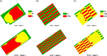
An indirect method for identifying uniform management zones, purportedly linked to yield potential and soil variability, was developed through a field-based clustering of multi-temporal satellite data, in the context of the European FP7 Project ERMES (www.ermes-fp7space.eu; Busetto et al., Reference Busetto, Casteleyn, Granell, Pepe, Barbieri and Campos-Taberner2016). The methodology, implemented in IDL and ENVI (Harris Corp., Melbourne, FL, USA) consists of three main processing steps, using spectrally and spatially coherent Landsat 7 and Landsat 8 resampled archive imagery of the last 5 years. In the first step, images were atmospherically corrected using the FLAASH tool based on MODTRAN4 in ENVI. Each image was then spatially resampled (bilinear method) to a higher spatial resolution of 5 m/pixel. Field based cloud masking was applied. Orthorectification and co-registration between the Landsat reflectance images and the field boundaries was performed, to assure geometric consistency between the images of the time-series. The second step was devoted to the separation of the vegetation and soil images in the time series of each agricultural field. To this aim, the Normalized Difference Vegetation Index (NDVI) was calculated using band 3 (red) and 4 (NIR) for Landsat 7 and band 4 (red) and 5 (NIR) for Landsat 8. Each field was classified as vegetation or soil on the basis of the percentage of pixels respectively exceeding or not a threshold NDVI value of 0.6. It should be noted that this procedure does not take into account the type of crop occurring in the field, which change from year to year . The third processing step consists of applying to these layers specific indices, suitable to describe soil and vegetation variability at the field scale. In the present study, targeted at developing N fertilization prescription maps, only vegetation images were employed, using NDVI as an index. Before applying a clustering procedure, a Z-score spatial normalization (Huang et al., Reference Huang, Goward, Masek, Zhiliang Zhu and Vogelmann2010) was performed on the NDVI layers, to allow comparability of images acquired on different dates and years. By using this normalization, the pixels of each field have zero mean and standard deviation of one on each date, making them independent from the crop species and growth stages and satellite acquisition conditions. The last step of the procedure consisted of applying the standard K-means algorithm, a simple but effective non-hierarchical clustering algorithm (Jain, Reference Jain2010). For each field three constant pattern classes were thus obtained (Fig. 1A): low mean values (L), median mean values (M), high mean values (H). It was assumed that these areas represented respectively low, average and high yield potential uniform management zones (UMZ).
Constant pattern maps (A) of fields B011 (top) and B012 (bottom), showing high (H), median (M) and low (L) yield potential zones; experimental layout (B) showing plots receiving the variable rate (VRA) or uniform (U) fertilisation treatments; the N rates finally applied (C): 92, 138 or 161 kg N ha−1, i.e. an intersection between (A) and (B). The U treatment received 138 kg N ha−1.

Field experiment on N fertilisation
The potential use of the results from the clustering procedure described above, for drawing N fertilization prescription maps was evaluated in a field trial on silage maize in 2016. The experiment took place in the commercial farm Maccarese S.p.A. (Fiumicino, Roma, Italy) (lat 41°52’38’’N, long 12°13’51’’E, 8.7 m a.s.l.), in two fields, coded as B011 and B012, of 7.88 ha and 13.48 ha respectively. The sites were located in a flat coastal land area and irrigated by a fixed system. The B011 field had on average 52.7% clay, 33.6% silt and 13.7%, sand, with an average soil organic matter of 3%, in the tilled layer (0-30 cm). B012 had 44.3% clay, 39.4% silt and 16.2% sand, with an average SOM of 3.3%. Both fields were cultivated in the same way according to the standard farm practice and sown on the 20th of May 2016 with the silage maize hybrid DKC 6237.
Prescription maps for the nitrogen fertilization were created for the B011 and B012 fields, assuming UMZs to be coincident with the constant patterns retrieved by the satellite data clustering procedure described above. The farm manager decided empirically, for both B011 and B012, the fertilization rates to be allocated to the different UMZs at the first application, i.e. at the two leaf stage (V2): the low yield potential areas (L clusters) received 92 kg N ha−1, M areas 138 kg N ha−1 and the H clusters 161 kg N ha−1 as urea.
This variable rate application (VRA) was compared to the uniform fertilization rate of 138 kg N ha−1 carried out at the farm. An experimental design was laid out, optimized for the subsequent geospatial analysis of the results by means of a pseudo cross-variogram and a standardized ordinary co-kriging methodology (Bishop and Lark, Reference Bishop and Lark2006). Both fields were subdivided into rectangular plots, each with an area of 20 mx100 m, according to a regular grid, alternating between variable rate and uniform fertilization treatments (Fig. 1B). This method enables the extrapolation over the whole fields of the yields resulting from both VR and uniform fertilized strips, in order to analyse, on a spatial basis, the statistical significance of the differences between the two treatments.
Prescription maps (Fig. 1C), drawn according to such experimental design, were uploaded to a tractor equipped with an Amazone ZA-M Profis Hydro S500 variable rate spreader, with an Amatron 3 control terminal. On June the 16th 2016 the first fertilisation was performed on B011 and B012 according to the prescription map. The second fertilisation was applied at the V6 stage on July the 10th 2016 with a uniform rate of 92 kg N ha−1 as urea throughout the whole field.
The two fields were harvested on 14-15 September 2016 by a forage harvester (New Holland FR700) equipped with a yield monitoring system composed by a volumetric sensor, a NIR moisture sensor, DGPS navigating and control system. Yield maps were post-processed filtering out errors and then pseudo-cross variograms were computed and a standardized ordinary co-kriging was applied. Yield maps for both the uniform and VRA fertilization treatments were also obtained, as well as maps of their differences and of their statistical significance.
Assessment of soil properties of constant pattern classes
After harvest, both B011 and B012 fields were surveyed with the aim to characterise, for each UMZ, soil particle fractions (according to ISSS classification), organic matter content and total soil nitrogen content, using respectively the Spinger-Klee and the Kjeldhal method. A total of 60 soil sampling points was identified in the two fields, collecting 3 cores at 30 cm depth for each point. Samples falling within a yield potential class were then bulked, before carrying out soil analyses, which were replicated 3 times for each bulked sample. Soil analyses results were then assessed by one-way-ANOVA in order to examine possible differences in soil properties among the classes (UMZs).
Results
Constant patterns as related to soil properties
The results of the multi-temporal clustering procedure of Landsat images for the study area are presented in Fig. 1A. Showing the areas identified as potentially high (H), average (M) or low (L) yielding for the two fields. The first issue is to know whether these classes reflect differences in soil properties. The soil survey revealed that for the B011 field, no significant differences for clay, silt or sand values were found among the three areas, whereas significant differences emerged for soil organic matter (SOM) and total soil N. On average SOM was 2.78% for the L area, 2.81% for the M and 3.29% for the H area (though significant differences existed only between H and the other areas). Soil N was 0.23 g kg−1 for L, 0.25 g kg−1 for M and 0.29 g kg−1 for H, similarly showing significant differences only between the high class and the others.
For B012, the ANOVA revealed significant differences for particle size distribution among the different areas: low and medium yield potential areas had significantly lower clay content (38.8% and 40.6%), as compared to the high potential, with 53.6% clay. Conversely, L and M had significantly higher silt (41.5% and 41.7%), than the H area which averaged 35.1% silt content. No significant differences were found for sand. Concerning the organic matter content, significant differences were found with higher values in areas classified as medium and high potential, (3.59% and 3.66% respectively), whereas a lower SOM of 2.73% was found in the L area. No significant differences appeared for total soil N in field B012 though.
Fertilization experiment results
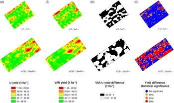
Using the pseudo co-kriging approach, the silage maize yields maps of the two fields for each fertilization treatment, i.e. uniform (U) or variable rate (VRA), were obtained (Fig. 2A and B). They represent the yield maps that would have been obtained if the U or the VRA treatments had been applied to the whole fields, respectively. For the B011 field, the maps for the two treatments showed an average yield estimate of 46.4 t ha−1 with the uniform rate treatment (Fig. 2A, top row), while for the variable rate fertilization (Fig. 2B, top row) the average yield was equal to 45.6 t ha−1, i.e. slightly less.
Results of the N fertilisation comparison between the VRA and U treatments, obtained from the pseudo co-kriging analysis for field B011 (top row) and B012 (second row), legends for the different maps are reported in the bottom row. (A): yield maps extrapolated to the whole field, from values collected in U strips. (B): yield maps extrapolated to the whole field, from values collected in VRA fertilization strips. (C): difference map between the (A) and (B) yield maps. (D): statistical significance map for yield differences of map (C).

Yields were highest in the H areas followed by M and L, in both fields and for both the VRA and U maps. Since the latter represent the case of a uniform fertilisation, this confirms the validity of the within-field constant patterns clustering method based on remote sensing data. In the U map of the B011 field, average yields of 48.7, 47.1 and 40.9 t ha−1 were obtained respectively in the H, M and L areas. In the B012 field yields were 49, 42.3 and 40.9 t ha−1 in the H, M and L areas, respectively.
A difference yield map (Fig. 2C) was calculated from the difference between the VRA and U yield maps. This map highlights areas performing better with the U (depicted in black) or with the VRA (depicted in white) treatment. In the B011 as a whole, higher yield for uniform fertilization accounted for 58% of the field area, while VRA performed better than U in 42% of the field. The differences between the VRA and U yields were statistically significant only in some areas of the field, as shown by a map of the level of significance (Fig. 2D). Areas with no significant differences between the two fertilization approaches are depicted in blue in Fig. 2D (top row) accounting for 85% of the overall B011 field area, whereas areas with a significant difference, depicted in orange or red in Fig. 2D, represent only 15% of the area. Of the areas showing a significant difference, only 6% show a positive difference, i.e. the VR fertilization outperforms the U, whereas for the remaining 9% it is the opposite.
For the B012 field, the uniform (Fig. 2A, second row) fertilisation provided an average yield estimate of 45 t ha−1, while the variable rate fertilization treatment (Fig. 2B, second row) resulted in an average yield of 45.4 t ha−1. For this field, the yield difference map (Fig. 2C, second row), showed that in 52% of the area VRA yields were higher than U, whereas for 48% it was the opposite. The significance map (Fig. 2D, second row) revealed that these differences were not significant for 51% of the field area. Significant differences, depicted in orange or red in Fig. 2D, represent in this case 49% of the field surface, of which 28% with variable rate fertilization outperforming the uniform one (positive difference), whereas 21% with a negative difference.
Discussion and conclusions
The clustering procedure based on the analysis of field-normalized NDVI time series from Landsat imagery, although taking into account only vegetation images, could identify areas with different soil properties. In general, the areas identified as potentially high yielding had higher soil organic matter as compared to medium or low potential areas. These preliminary results call for further and more extensive studies to better understand the relationship between soil properties and the constant patterns revealed by the clustering procedure. It could be argued that soils are only one component of the information contributing to the constant pattern map creation, but it cannot be neglected that they are a major factor controlling the vegetation vigour, which is the other multi-annual information exploited in the clustering procedure.
The field trial had the purpose of investigating whether the patterns identified could be used as prescription maps for VRA of N fertiliser in silage maize. This assessment of the usefulness of VRA fertilization regulated by constant patterns maps cannot be considered conclusive. In fact, the yield differences between those estimated for variable rate against those for the uniform fertilization, do not demonstrate significant advantages for VRA. Only 49% of the B012 field area show a significant difference in maize yield (of which 28% was positive), whereas for B011 this is reduced to merely 15% (with 6% positive).
It is evident, considering the confidence map results that the different N rates did not bring about large significant variability in yield. It should be noted that urea fertilizer quantities where empirically determined by the farm manager and not planned according to an N balance. The N rates chosen, actually differed only by 20-25 kg N ha−1. Small yield difference might have also passed undetected due to the error introduced by the harvest recording system, in the order of 16% as assessed by a specific calibration activity on the forage harvester carried out at the farm.
These results could be considered encouraging regarding fertilization based on constant patterns for silage maize, particularly as other proximal and remote sensing techniques are hindered by the early development stages (V2 and V6) when fertilization has to be performed. In addition, this study could represent a starting point for the use of satellite time series to recognise yield potentials, and suggest a further testing on other sites for the application of precision agriculture practises, in order to improve crop production whilst reducing environmental impact.