





Non-technical Summary
Studying the relationship between morphological traits and their ecological context provides a means to predict how extinct species interacted with their environments. Traditional statistical approaches for comparing morphological differences among ecological groups and classifying fossils, however, are limited, especially with the increasing prevalence of complex, multidimensional datasets. These methods often require unrealistic sample sizes and do not always account for the influence of shared ancestry on traits. To address these key challenges, we present Bayesian ordinal regression models to classify modern African bovids (cows, goats, antelopes, and their relatives) among four habitat categories, based on differences in shape in the astragalus, one of the bones of the ankle. Our results show that the Bayesian models can correctly classify bovids at rates either meeting or exceeding traditional methods such as canonical variates analysis, especially when including information about species relatedness. However, without information about the species’ ancestry, classification success rates decrease dramatically. These results suggest that removing information about how species relatedness influences shape can be detrimental to the aim of generating accurate predictions. Deciding whether to correct for the influence of shared ancestry thus depends on the study aim. The Bayesian modeling results presented here highlight how this methodology can lead to more robust, nuanced conclusions about the relationship between traits and ecology, which can be applied to improve our understanding of the evolution of extinct species.
Introduction
Ecomorphology, or the study of how morphology relates to the functional demands of certain ecological variables (Karr and James Reference Karr, James, Cody and Diamond1975; Bock Reference Bock1990), is a powerful tool in paleontology and neontology. Ecomorphology is rooted in concepts of adaptation and convergence that are fundamental to evolutionary biology and assume that species will evolve in response to their environments to maximize performance and, ultimately, their reproductive fitness (Darwin Reference Darwin1859; Arnold Reference Arnold1983). This implies that species should convergently evolve similar features if they inhabit similar environments. As a result, links between specific morphological features and ecological variables of interest in extant taxa, such as habitat preference, diet, or locomotor behavior, can be used to infer those traits that cannot be directly observed in fossil species.
To describe the ways in which morphological features are linked to function, and to predict function in extinct taxa, researchers often employ canonical variates analysis (CVA). CVA, also commonly referred to as linear discriminant function analysis (DFA or LDA; e.g., Rencher Reference Rencher1992) is a multivariate classification method that estimates linear dimensions of maximal separation among specified groups in a dataset by maximizing the ratio of between-group variance to within-group variance (Mitteroecker and Bookstein Reference Mitteroecker and Bookstein2011; Zelditch et al. Reference Zelditch, Swiderski and Sheets2012). The use of CVA is particularly common in the context of 3D geometric morphometric (GM) analyses, as it facilitates interpretations of morphological variation within complex, high-dimensional datasets (Bookstein Reference Bookstein1991; Adams et al. Reference Adams, Rohlf and Slice2004; Mitteroecker and Bookstein Reference Mitteroecker and Bookstein2011). However, CVA is unlikely to be the most appropriate method for analyzing high-dimensional 3D GM data, as its underlying assumptions are frequently violated in biological datasets (Mundry and Sommer Reference Mundry and Sommer2007; Kovarovic et al. Reference Kovarovic, Aiello, Cardini and Lockwood2011; Mitteroecker and Bookstein Reference Mitteroecker and Bookstein2011). Despite this, CVA remains commonly applied to investigate ecomorphological questions (e.g., Chen and Wilson Reference Chen and Wilson2015; Grossnickle et al. Reference Grossnickle, Chen, Wauer, Pevsner, Weaver, Meng, Liu, Zhang and Luo2020; Anderson et al. Reference Anderson, Kovarovic and Barr2024; Malherbe et al. Reference Malherbe, Webb, Palisson-Kramer, Ndiema, Braun, Haeusler and Forrest2025b; Orgebin et al. Reference Orgebin, Dziomber, Aiglstorfer and Mennecart2025), and as a result it is imperative to apply new methods that allow more appropriate inferences to be drawn from such complex datasets.
One major limitation of applying CVA in ecomorphology pertains to its large sample size requirements. Because CVA seeks to identify axes that maximally separate group centroids, with enough variables, a dataset can always be rotated in such a way that separates groups, even if the variation upon which groups are separated is biologically irrelevant (Mitteroecker and Bookstein Reference Mitteroecker and Bookstein2011). Therefore, if the number of observations is not greater than the number of variables, it is more likely that the analysis will produce spurious results. To obtain robust discrimination among groups and reliable predictions of unknowns, CVA therefore requires that the number of observations be much greater than the number of variables in the dataset and, specifically, that the number of observations per group exceed the number of variables (Williams and Titus Reference Williams and Titus1988; Friedman Reference Friedman1989; Kovarovic et al. Reference Kovarovic, Aiello, Cardini and Lockwood2011; Mitteroecker and Bookstein Reference Mitteroecker and Bookstein2011). In 3D GM analyses of Procrustes-aligned landmark data, the number of variables is equal to 3k − 7, where k is the number of landmarks (Zelditch et al. Reference Zelditch, Swiderski and Sheets2012). When using a large number of landmarks to describe the shape of a particular structure, this sample size threshold for CVA is difficult if not impossible to meet, especially when analyzing fossil data (Kovarovic et al. Reference Kovarovic, Aiello, Cardini and Lockwood2011).
As a result, it is common practice in paleontology to first conduct a principal components analysis (PCA) on the landmark data and use a subset of the resulting principal components (PCs) as predictors in a CVA. Typical strategies for selecting which PCs to use include using only the first N PCs that account for a certain percentage of the sample variance (e.g., 90% or 95%), or using a broken stick algorithm to determine the number of PCs that account for a greater proportion of variance than expected by chance (Jackson Reference Jackson1993; Zelditch et al. Reference Zelditch, Swiderski and Sheets2012). However, this dimensionality reduction assumes that the most meaningful variance for discriminating among groups is thoroughly represented by the first few PCs, which can be true, but may not be generalizable to every dataset or question under investigation (Cardini and Elton Reference Cardini and Elton2008; Kovarovic et al. Reference Kovarovic, Aiello, Cardini and Lockwood2011).
The application of CVA to ecomorphology is further complicated by phylogeny. It is well established that species, or multiple observations of the same species, are not statistically independent because of their shared ancestry (Felsenstein Reference Felsenstein1985). Therefore, the discriminatory ability of a CVA can be inflated as a result of taxa belonging to the same ecological group and having similar morphologies due to their phylogenetic relatedness (Rohlf Reference Rohlf2006; Mundry and Sommer Reference Mundry and Sommer2007). In other words, CVA results cannot inform whether traits associated with a particular ecological group are functional, convergent, or simply due to ancestral retention (Uyeda et al. Reference Uyeda, Zenil-Ferguson and Pennell2018). One way of controlling for the phylogenetic non-independence of characters in a dataset is to first use phylogenetic generalized least squares (PGLS) regressions to examine relationships between predictor and grouping variables after adjusting for phylogenetic signal, and then only include the variables that show a significant correlation with the grouping variable in the CVA (Barr Reference Barr2014; Barr and Scott Reference Barr and Scott2014). This approach provides a useful means of establishing which variables have a significant functional relationship with the grouping variable even after adjusting for phylogeny and limits overfitting of the CVA by focusing on traits that show a signal of convergent evolution along distantly related branches of a phylogeny. However, this method may also be overly conservative, as functional traits associated with a particular ecology can be inherited from a common ancestor, and thus phylogenetic signal in a trait does not necessarily make it uninformative for ecomorphology (Plummer et al. Reference Plummer, Ferraro, Louys, Hertel, Alemseged, Bobe and Bishop2015; Elton et al. Reference Elton, Jansson, Meloro, Louys, Plummer and Bishop2016).
An alternative means of adjusting for phylogenetic signal in discriminant analyses is a phylogenetic flexible discriminant analysis (pFDA) (Motani and Schmitz Reference Motani and Schmitz2011). A flexible discriminant analysis (FDA) is a nonparametric form of discriminant analysis in which the linear regression used to define maximal separation among groups is replaced by a nonlinear regression function (Hastie et al. Reference Hastie, Tibshirani and Buja1994). In pFDA, the linear regression is replaced by PGLS (Motani and Schmitz Reference Motani and Schmitz2011; Serio et al. Reference Serio, Brown, Clauss and Meloro2024) making it not a true FDA, as PGLS is a linear function, though it could be extended as such. Thus, like CVA, the aim of pFDA is to estimate axes of maximal separation among groups within the data, but unlike CVA, pFDA corrects for phylogenetic signal by rescaling the data using an estimated optimal Pagel’s λ value (Motani and Schmitz Reference Motani and Schmitz2011). This method is advantageous, because it adjusts for phylogenetic signal in the grouping variable, not just the predictors, as ecological categories are also likely to be passed from ancestors to descendants (Motani and Schmitz Reference Motani and Schmitz2011; Elton et al. Reference Elton, Jansson, Meloro, Louys, Plummer and Bishop2016). Additionally, application of pFDA permits inclusion of the full dataset, without the removal of variables that do not meet a significant p-value threshold in PGLS. However, pFDA requires that each species only be represented by a single observation (Motani and Schmitz Reference Motani and Schmitz2011; Elton et al. Reference Elton, Jansson, Meloro, Louys, Plummer and Bishop2016; Serio et al. Reference Serio, Brown, Clauss and Meloro2024), meaning that potentially informative intraspecific variation in a dataset must be averaged in order to apply the analysis. Additionally, using pFDA to predict ecological traits for fossils is only possible when the fossils can be assigned to a species within the phylogeny. This means that its application in ecomorphological studies is limited, as often the elements used for ecomorphology in the fossil record cannot be identified to the species level (e.g., isolated bovid postcranial elements).
Existing methods applied to ecomorphological questions are thus limited in their ability to handle uneven sampling and confounding phylogenetic factors while also being unable to account for important intraspecific variation. Here, we present an alternative approach using Bayesian multilevel modeling to address the aforementioned concerns. Bayesian methods describe model parameters in terms of probability distributions, which are estimated given a set of assumptions about the data called priors (McElreath Reference McElreath2020). Bayesian models are not limited by sample size or model assumptions in the same way that traditional statistical methods are, as the uncertainty caused by limited sampling will be reflected in the width of the posterior probability distribution of the model estimates, and assumptions about the underlying distribution of the data given existing knowledge are explicitly defined as priors. Multilevel Bayesian models provide an additional advantage for handling uneven sampling among groups and repeat sampling without averaging the data, as they pool information across clusters in the data to improve parameter estimates and reduce overfitting (McElreath Reference McElreath2020). This means that models can analyze multiple samples per species by including a grouping variable that corresponds to species and can covary according to phylogeny. A Bayesian multilevel framework is thus well suited for investigating ecomorphology using 3D GM data, as the models can account for sampling of multiple individuals per species and incorporate information about phylogenetic covariance in the dataset in the model priors (Nations et al. Reference Nations, Heaney, Demos, Achmadi, Rowe and Esselstyn2019; McElreath Reference McElreath2020). For example, previous studies have used Bayesian multilevel modeling with phylogenetic effects to obtain insights into the dietary ecology of fossil primates (Fulwood et al. Reference Fulwood, Shan, Winchester, Gao, Kirveslahti, Daubechies and Boyer2021) and carnivorans (Wisniewski et al. Reference Wisniewski, Nations and Slater2023) using tooth morphology and to investigate which skeletal traits best predict locomotor mode in rodents after accounting for phylogenetic relatedness (Nations et al. Reference Nations, Heaney, Demos, Achmadi, Rowe and Esselstyn2019). This modeling approach thus provides a promising method for disentangling the influences of phylogeny and ecology on morphology to generate more informed predictions of ecology in fossils.
As a case study, we generate Bayesian ordinal models to investigate the relationship between extant African bovid astragalus morphology and habitat category. Bovids are commonly analyzed in the context of ecomorphology and paleoenvironmental reconstruction owing to their abundance in extant and fossil assemblages and their habitat specificity, which is the tendency for each extant species to occupy a generally predictable habitat within the continuum of open grassland and closed forests in Africa (Scott Reference Scott1979; Greenacre and Vrba Reference Greenacre and Vrba1984; Kappelman Reference Kappelman1988; Plummer and Bishop Reference Plummer and Bishop1994; DeGusta and Vrba Reference DeGusta and Vrba2003; Plummer et al. Reference Plummer, Bishop and Hertel2008; Barr Reference Barr2014). A wealth of research confirms that because of this broadly defined habitat specificity, several elements of the bovid postcranial skeleton, including the astragalus, demonstrate functional relationships with habitat (Kappelman Reference Kappelman1988; DeGusta and Vrba Reference DeGusta and Vrba2003; Plummer et al. Reference Plummer, Bishop and Hertel2008; Barr Reference Barr2014; Dunn and Avery Reference Dunn and Avery2021; Anderson et al. Reference Anderson, Kovarovic and Barr2024; Malherbe et al. Reference Malherbe, Webb, Palisson-Kramer, Ndiema, Braun, Haeusler and Forrest2025b). Importantly, too, while there is a significant influence of allometry on astragalus shape, astragalus size does not vary among habitat categories, and several metrics of the astragalus have been shown to still significantly vary with habitat after correcting for body size (Barr Reference Barr2014; Wimberly Reference Wimberly2023; Orgebin et al. Reference Orgebin, Dziomber, Aiglstorfer and Mennecart2025; Kelly and Alemseged Reference Kelly and Alemseged2026). Therefore, we first develop models that examine the relationship between habitat and astragalus shape with the expectation that there should be clear distinctions in astragalus shape that are related to habitat-specific functional demands. We also apply CVA to the same data to compare with the predictive ability of our Bayesian models.
Bovids also demonstrate high phylogenetic signal in their morphology and habitat preferences, and as a result, much of the debate on how to appropriately address phylogenetic signal in ecomorphological studies centers around bovids (Klein et al. Reference Klein, Franciscus and Steele2010; Louys et al. Reference Louys, Montanari, Plummer, Hertel and Bishop2013; Barr and Scott Reference Barr and Scott2014; Scott and Barr Reference Scott and Barr2014; Elton et al. Reference Elton, Jansson, Meloro, Louys, Plummer and Bishop2016; Orgebin et al. Reference Orgebin, Dziomber, Aiglstorfer and Mennecart2025). We generate additional Bayesian models that include a phylogenetic grouping variable to assess the impact of accounting for phylogeny on their predictive ability. For comparison, we also apply a pFDA to the data. We expect that including a phylogenetic parameter in the Bayesian model will improve predictions, given the known association between habitat and phylogeny in bovids, but it may not improve habitat predictions for unknown species, as the phylogenetic signal will be separated from the predictor variables. Altogether, we aim to provide a more robust framework for analyzing ecomorphological data and discriminating among groups and to shed new light on the question of whether phylogenetically non-independent characters should be used to investigate ecomorphology.
Materials and Methods
Dataset
We analyzed a sample of 136 adult, wild African bovid astragali from the mammal collections of the Field Museum of Natural History, representing 36 species across 10 tribes (Kelly and Alemseged Reference Kelly and Alemseged2026). Each individual was assigned to one of four habitat categories: Open (n = 52), Light Cover (n = 48), Heavy Cover (n = 24), or Forest (n = 12), according to its species assignment and corresponding habitat groupings used in the literature (Kappelman et al. Reference Kappelman, Plummer, Bishop, Duncan and Appleton1997; DeGusta and Vrba Reference DeGusta and Vrba2003; Kovarovic and Andrews Reference Kovarovic and Andrews2007; Plummer et al. Reference Plummer, Bishop and Hertel2008; Barr Reference Barr2014). Specimens were surface scanned using a Creaform Go!Scan 3D scanner at 0.3 mm resolution, and 3D meshes were generated in VXElements (Creaform Inc. Reference Inc2023). Astragali from Madoqua species (n = 5) were too small to scan using the Go!Scan, and were therefore instead scanned using a Capture Mini Scanner, and 3D meshes were generated using Geomagic Design X (3D Systems, Inc. 2023). Any small holes in the meshes were filled, and any connective tissue was digitally removed from all specimens in Geomagic Design X (3D Systems, Inc. 2023). All 3D meshes used in this study are archived on MorphoSource (https://doi.org/10.17602/M2/L861199).
In a previous paper (Kelly and Alemseged Reference Kelly and Alemseged2026), we captured the shape of the astragalus using 20 fixed landmarks (Supplementary Fig. 1) placed on each 3D mesh, and we use the same landmark data here. All subsequent statistical analyses were performed on the landmark data using R v. 4.4.3 (R Core Team 2025), and all code generated to run the analyses is available on Zenodo (https://doi.org/10.5281/zenodo.22680231). We performed a generalized Procrustes analysis on the landmark coordinates to scale them to a uniform centroid size and correct for transformations, translations, and rotations in the data (Gower Reference Gower1975; Webster and Sheets Reference Webster and Sheets2010), using the R package geomorph (Adams et al. Reference Adams, Collyer, Kaliontzopoulou and Baken2021). The resulting Procrustes coordinates were subjected to a PCA to summarize the shape variation in the sample in terms of a set of derived orthogonal axes, or PCs (Zelditch et al. Reference Zelditch, Swiderski and Sheets2012). A broken stick algorithm was then used to determine which PCs represented a greater proportion of sample variance than expected by chance (Jackson Reference Jackson1993).
Bayesian Ordinal Regression Models
We generated Bayesian ordinal regression models to test how well the PC scores derived from the Procrustes-aligned 3D landmarks of bovid astragali can predict habitat group. We use ordinal regressions here, as the four habitat categories have a natural order in terms of the amount of tree cover in the habitat, ranging from lowest in the Open category, to highest in the Forest category, and ordinal models assume that change in one direction in any predictor variable should be associated with progression through the categories (McElreath Reference McElreath2020). For example, increasingly proximodistally short astragali are expected to be associated with increasingly open habitats (DeGusta and Vrba Reference DeGusta and Vrba2003; Plummer et al. Reference Plummer, Bishop and Hertel2008; Barr Reference Barr2014). This relationship can be modeled with a linear equation, where change in the predictor variables determines the cumulative probability of belonging to one of the four habitat categories.
We first generated three models to investigate the influence of including different numbers of PCs as predictor variables, without including a phylogenetic effect in the model, thereby treating each sampled individual as an independent observation, irrespective of species identity. The first model used all PCs to consider the full extent of shape variation in the sample. The second model used only those PCs that cumulatively account for 95% of the sample variance to mimic a typical percent variance cutoff used in GM studies (Zelditch et al. Reference Zelditch, Swiderski and Sheets2012). The third model used only the PCs that were deemed significant according to the broken stick algorithm, as these PCs are more likely to represent signal versus noise in the data (Jackson Reference Jackson1993). Values along each PC were centered at zero and scaled to a standard deviation of one (z-score) to facilitate each model’s exploration of the posterior distribution (McElreath Reference McElreath2020). The distribution of habitat categories is described as an ordered categorical distribution:

The vector p represents the set of probabilities of membership in each habitat category and is derived from the vector of cumulative probabilities q, which represent the probability of membership in each category or those below it. The cumulative distribution is divided into K = 4 groups separated by K – 1 = 3 thresholds, or intercepts, which mark the borders between groups (Bürkner and Vuorre Reference Bürkner and Vuorre2019; McElreath Reference McElreath2020). The probability (p) of each successive habitat category (k) is described as:


The linear model to describe the cumulative probability of membership in each habitat group in relation to astragalus morphology is given by the equation:


The logit link function is used here to restrict cumulative probabilities between zero and one, and as a result, the parameters estimated by the model are given in the log-odds scale. The α k parameter represents the intercept for each successive habitat category (k). The φ i parameter represents the linear model that describes the relationship between the PC scores for each individual, i, multiplied by the slope for each PC (β). Finally, we set regularizing priors on the model parameters as follows, and conducted prior predictive checks to confirm that the priors were constrained to realistic values and not biased in any direction:


One benefit of Bayesian multilevel models over traditional classification procedures is that it is trivial to estimate and account for both phylogenetic and intraspecific effects using group-level effects. To evaluate the degree to which phylogenetic covariance may influence predictions of habitat use in bovids, we generated a second suite of models that include a phylogenetic group-level effect defined by a phylogenetic covariance matrix derived from a time-calibrated molecular phylogeny of Cetartiodactyla (Zurano et al. Reference Zurano, Magalhães, Asato, Silva, Bidau, Mesquita and Costa2019). One rare species that is present in our morphological dataset, Ammodorcas clarkei, was not included in this phylogeny and was inserted as a sister taxon to Litocranius walleri, according to its placement in a separate phylogeny of the tribe Antilopini (Bärmann et al. Reference Bärmann, Rössner and Wörheide2013; Bärmann Reference Bärmann2014). With this phylogeny, we then computed a scaled phylogenetic covariance matrix in which diagonal elements represent evolutionary variances (root-to-tip distances for each taxon) and off-diagonal elements represent evolutionary covariances (shared root-to-common ancestor distances for each pair of taxa) using the vcv.phylo function from the ape R package (Paradis and Schliep Reference Paradis and Schliep2019). The model syntax remained the same as the non-phylogenetic models, except for the φ i parameter, which was updated to include a phylogenetic group-level effect (Rphylo) which varies according to the phylogenetic covariance matrix and an additional species group-level effect (Sspecies) to account for any additional variability resulting from sampling multiple individuals per species (de Villemereuil and Nakagawa Reference Villemereuil, Nakagawa and Garamszegi2014):

The Rphylo and Sspecies parameters are both normally distributed, with means of zero and standard deviations σ phylo and σ species, respectively. The difference between the two parameters is that the σ phylo parameter is multiplied by the scaled covariance matrix derived from the phylogeny so that the Rphylo effects are correlated based on the phylogeny, while the Sspecies effects vary independently of the phylogeny (de Villemereuil and Nakagawa Reference Villemereuil, Nakagawa and Garamszegi2014). Both σ parameters are given a prior that allows both group-level effects to vary widely:

Using the posterior parameters from the phylogenetic models, we also estimated the phylogenetic signal in the data by calculating the variance of the phylogenetic terms in the model divided by the sum of the variance in the phylogenetic and non-phylogenetic terms (Bürkner Reference Bürkner2021; Pearse et al. Reference Pearse, Davies and Wolkovich2025). This provides an estimate of the proportion of sample variance attributable to phylogeny, and it can be interpreted similarly to Pagel’s λ, where values closer to one indicate greater phylogenetic signal, although the two metrics are not computationally equivalent (Pearse et al. Reference Pearse, Davies and Wolkovich2025).
All models were fit using the R package brms (Bürkner Reference Bürkner2017, Reference Bürkner2018, Reference Bürkner2021). Each model was fit using four Markov chain Monte Carlo (MCMC) chains with 3000 posterior draws each, with the first 1500 warm-up draws excluded. Convergence of MCMC chains was assessed using the R-hat
$ \left(\hat{R}\right) $
 statistic, where a value of one indicates convergence and successful exploration of the posterior distribution (Gelman and Rubin Reference Gelman and Rubin1992).
Predictive performance of each model was assessed in several ways. For each model, we used parameters derived from 1000 random draws from the posterior to classify each specimen in the dataset according to the habitat category with the maximum posterior probability. Based on these posterior predictions, we calculated the percentage of correct re-classifications for each model. We also calculated a weighted sum posterior probability of group membership for each specimen as:

This indicates where each specimen lies within the full cumulative probability distribution and provides an estimate of the uncertainty around categorical predictions. For the phylogenetic models, we calculated the percentage of correct classifications and weighted sums both including and excluding the phylogenetic group-level effects from the predictions. Phylogenetic group-level effects were excluded to mimic predictions in cases where the taxonomy is unknown, as is the norm for fossil bovid astragali. Additionally, as leave-one-out cross-validation is computationally intensive for Bayesian models, we approximated how well each model is expected to predict out-of-sample observations using the widely applicable information criterion (WAIC; McElreath Reference McElreath2020). This metric provides an assessment of overfitting risk and penalizes models that include greater numbers of parameters.
CVA
To compare our Bayesian models with traditional statistical approaches, we also ran CVAs on the PC scores of all 136 individuals, as well as on species mean PC scores. To generate species mean PC scores, we first estimated species mean astragalus shapes. We conducted a generalized Procrustes analysis on the astragali within each species, then computed a mean shape based on the species-specific Procrustes-aligned coordinates using the mshape function in geomorph (Adams et al. Reference Adams, Collyer, Kaliontzopoulou and Baken2021). We then conducted a second generalized Procrustes analysis on the species mean shapes, then ran a PCA on the resulting Procrustes coordinates. A broken stick algorithm was then applied to the resulting species mean PCs. With both datasets, we conducted three CVAs: one using all the PCs, which is equivalent to using the full Procrustes shape; a second using the first PCs that account for 95% of sample variance, a commonly adopted cutoff; and a third using only the broken stick significant PCs. All CVAs were subjected to leave-one-out cross-validation to assess their correct classification ability.
pFDA
As CVA does not permit any means of accounting for phylogenetic signal in the data, we performed a pFDA to assess how correcting for phylogenetic non-independence of data points influences discriminatory ability. pFDA is similar to a linear canonical variates or discriminant analysis, but accounts for the phylogenetic non-independence of data points by defining the discriminant axes based on PGLS regression, rather than ordinary least squares (OLS) regression (Motani and Schmitz Reference Motani and Schmitz2011; Serio et al. Reference Serio, Brown, Clauss and Meloro2024). To perform the pFDA, we used species mean PC scores, as pFDA requires that each species be represented by a single observation. The same phylogeny as was used in the Bayesian models was used for the pFDA. When applied to the data, the pFDA procedure estimates an optimal Pagel’s λ for both the predictor and categorical variables that minimizes the residual sum of squares error in the model. This optimal λ is then used to transform the branch lengths of the phylogeny and generate discriminant axes (DAs) using PGLS that maximize separation among groups (Motani and Schmitz Reference Motani and Schmitz2011). As with the CVA, we ran the pFDA on all of the PCs; the first PCs that account for 95% of the species mean sample variance; and the PCs that were significant according to a broken stick model. Leave-one-out cross-validation was performed on all three pFDAs to assess their classification performance.
Results
Non-phylogenetic Models
The Bayesian models that do not include phylogenetic or species-level effects reliably classify bovids into the four ranked habitat categories based on astragalus shape (Fig. 1). Moreover, the non-phylogenetic models highlight that ecomorphologically important shape variation is not limited to the first few PCs. For each model, predictive performance was assessed by applying the model to the input data to classify each individual using parameters generated from 1000 random draws from the model. Individuals were classified into the group for which they had the greatest posterior probability of membership. Increasing the number of PCs included as predictors generally increased predictive accuracy. The model using only the PCs that were significant according to a broken stick algorithm, PCs 1–8, had a 67.6% correct classification rate. Increasing the number of PCs to the first 30, which represent 95% of the sample variance, yields a correct classification rate of 73.5%. The model that used all 53 PCs had the highest correct classification rate, at 80.9%. WAIC scores for the three models are very similar, but the model using PCs 1–30 has the lowest score, and therefore the least overfitting risk (Table 1).
Posterior predictive plots for three Bayesian ordinal regression models that do not include a phylogenetic grouping variable and thus consider each astragalus as an independent observation irrespective of species identity. The plots depict reconstructed habitat categories for the astragali used to generate the model (n = 136). Models varied in the number of principal components (PCs) included as predictors: PCs 1–8, which were significant according to a broken stick algorithm (A, D); PCs 1–30, which represent 95% of sample variance (B, E); and PCs 1–53, which are the full dataset (C, F). The percentage of individuals reclassified correctly by the model is shown below each column. (A–C) Bar plots separating the dataset according to known habitat category, with each bar colored according to the model’s predicted habitat for the members of that habitat group. Across the three models that used varying numbers of PCs as predictors, posterior predictions are most accurate for the Open group, and least accurate for Forest habitat bovids. (D–F) Scatter plots indicating the range of weighted sum posterior probabilities of group membership for each individual bovid within each habitat group. Points are colored according to the habitat group that had the greatest individual posterior probability for that individual. F, Forest; HC, Heavy Cover; LC, Light Cover; O, Open.

Figure 1. Long description
A six-panel figure organized into two rows and three columns.
Top Row (Panels A, B, C): Stacked bar charts showing the count of individuals on the y-axis (0 to 50) against known habitat on the x-axis (O for Open, L C for Light Cover, H C for Heavy Cover, F for Forest), colored according to predicted habitat.
- Panel A (P Cs 1-8): Shows high misclassification in the Forest group, with many individuals predicted as L C or H C. The correct posterior classification rate is 67.6 percent.
- Panel B (P Cs 1-30): Shows improved classification, particularly in the Forest group. The correct posterior classification rate is 73.5 percent.
- Panel C (P Cs 1-53): Shows the highest alignment between known and predicted habitats, with the Forest group showing a dominant dark green segment for correct prediction. The correct posterior classification rate is 80.9 percent.
Bottom Row (Panels D, E, F): Scatter plots showing the weighted sum of posterior probabilities on the y-axis (1 to 4) against known habitat on the x-axis.
- Panel D (P Cs 1-8): Points are widely dispersed vertically within each habitat category, indicating lower confidence.
- Panel E (P Cs 1-30): Points begin to cluster more tightly at higher y-axis values for their respective categories.
- Panel F (P Cs 1-53): Points show the tightest vertical clustering and highest separation between groups.
Legend: Colors represent predicted habitats: Brown for O, Tan for L C, Light Green for H C, and Dark Green for F.
Widely applicable information criterion (WAIC) scores, effective number of parameters (pWAIC), and standard error of WAIC scores for the three models using principal components (PCs) only to predict habitat category. Models are arranged from lowest to highest WAIC score, with the lowest WAIC scores indicating the least overfitting risk

Table 1. Long description
The table consists of four columns: Model, W A I C, p W A I C, and S E W A I C.
* Row 1: Model P Cs 1–30 has a W A I C of 232.2, a p W A I C of 24.3, and an S E W A I C of 14.1.
* Row 2: Model P Cs 1–8 has a W A I C of 234.5, a p W A I C of 7.5, and an S E W A I C of 14.5.
* Row 3: Model P Cs 1–53 has a W A I C of 235.0, a p W A I C of 39.2, and an S E W A I C of 15.1.
The models are ordered by increasing W A I C score, indicating that the P Cs 1–30 model has the lowest risk of overfitting.
We also examined where each individual falls along the cumulative distribution by calculating its weighted sum posterior probability (Fig. 1D–F). The weighted sums indicate that although an individual may correctly have the highest probability of membership in its known habitat group, its cumulative probability can vary, and there is considerable overlap among groups. Notably, in the model with all 53 PCs, some individuals in the Forest group were correctly reclassified as Forest when the highest individual probability was considered, but their weighted sum probability overlaps with individuals that were correctly classified in the Heavy Cover category (Fig. 1F).
All three models performed best at classifying astragali in the Open habitat category. The addition of more PCs improved predictions most notably for the Heavy Cover and Forest groups. This indicates that the PCs that represent the greatest proportion of sample variance (the lower PCs) primarily capture the difference between Open habitat bovids and all others, while the differences separating the other three groups are more subtle and are represented on higher PCs that individually capture a smaller proportion of sample variance.
The percentage of correct posterior predictions from the Bayesian results are comparable to, and sometimes greater than, the cross-validated classification rates of the CVAs generated with the same subsets of PCs. As with the Bayesian models, classification accuracy improves with the addition of more PC variables (Fig. 2). Compared with the Bayesian models using the same PCs, the CVA with the first 8 PCs returned a similar, but slightly greater leave-one-out cross-validated classification rate of 69.1%, as did the CVA using the first 30 PCs, which had a classification rate of 74.3%. The CVA with all 53 PCs, however, had a lower cross-validated classification rate than the Bayesian model using all PCs, at 76.5%. The variation along CV1, which represents the greatest proportion of the variance in all three analyses, also suggests that bovid astragali in the Open category are the most distinct from all others, as they are consistently separated from the other three groups with little overlap.
Results from three canonical variates analyses (CVAs) using all individuals (n = 136) that vary in the number of principal components (PCs) used as input variables. In all scatter plots, individual points represent a single astragalus and are colored according to their known habitat category. The shape of each point indicates its tribe-level taxonomy. Leave-one-out cross-validation success rates are included for each model at the bottom of each column. (A, D) CV 1 vs. CV 2 and CV 1 vs. CV 3 for a model using only the PCs that were significant according to a broken stick algorithm (PCs 1–8). (B, E) CV 1 vs. CV 2 and CV 1 vs. CV 3 when the first 30 PCs, which represent 95% of the sample variance, are used as predictor variables. (C, F) CV 1 vs. CV 2 and CV 1 vs. CV 3 for a model using all 53 PCs as predictor variables.

Figure 2. Long description
A multi-panel figure containing six scatter plots arranged in two rows and three columns.
Top Row (C V 1 vs. C V 2):
* Panel A (P C s 1-8): X-axis C V 1 (88.7 percent), Y-axis C V 2 (8.9 percent). Shows significant overlap between habitat clusters.
* Panel B (P C s 1-30): X-axis C V 1 (71.5 percent), Y-axis C V 2 (17.3 percent). Clusters begin to separate, particularly the Open habitat group.
* Panel C (P C s 1-53): X-axis C V 1 (60.2 percent), Y-axis C V 2 (24.1 percent). Shows the clearest separation between Forest, Heavy Cover, Light Cover, and Open habitats.
Bottom Row (C V 1 vs. C V 3):
* Panel D (P C s 1-8): X-axis C V 1 (88.7 percent), Y-axis C V 3 (2.3 percent). High overlap among all groups.
* Panel E (P C s 1-30): X-axis C V 1 (71.5 percent), Y-axis C V 3 (11.1 percent). Improved separation of clusters.
* Panel F (P C s 1-53): X-axis C V 1 (60.2 percent), Y-axis C V 3 (15.7 percent). Distinct clustering with minimal overlap.
Classification Rates:
* Column 1 (A, D): 69.1 percent correct cross-validated classification rate.
* Column 2 (B, E): 74.3 percent correct cross-validated classification rate.
* Column 3 (C, F): 76.5 percent correct cross-validated classification rate.
Legend Details:
* Habitat (Colors/Hulls): Forest (dark green), Heavy Cover (light green), Light Cover (tan), and Open (brown).
* Tribe (Shapes): 11 distinct symbols representing Aepycerotini, Alcelaphini, Antilopini, Bovini, Caprini, Cephalophini, Hippotragini, Neotragini, Reduncini, and Tragelaphini.
Phylogenetic Models
When a phylogenetic group-level effect is included in the Bayesian ordinal regression models, the posterior predictions become extremely accurate (Fig. 3). The model fit with the first 8 PCs has a 97.8% correct posterior classification rate, similar to that of the model using PCs 1–30 (97.1%), and the model using all 53 PCs correctly classifies individuals into their habitat category 99.3% of the time. Comparison of WAIC scores among the three phylogenetic models suggests that the model using only PCs 1–8 has the least overfitting risk (Table 2). Estimates of phylogenetic signal from all three models, suggest that phylogenetic signal is moderate in the dataset, with mean estimated values between 0.59 and 0.66 (Table 3).
Posterior predictive plots for the three Bayesian ordinal regression models which account for phylogenetic covariance by including a phylogenetic grouping variable. The plots show reconstructed habitat categories for the astragali used to generate the model (n = 136). Models varied in the number of principal components (PCs) included as predictors: PCs 1–8, which were significant according to a broken stick algorithm (A, D); PCs 1–30, which represent 95% of sample variance (B, E); and PCs 1–53, which are the full dataset (C, F). The percentage of individuals reclassified correctly by the model is shown below each column. (A–C) Bar plots indicating the proportion of the dataset belonging to each habitat category, with each bar colored according to the model’s predicted habitat for the members of that habitat group. (D–F) Scatter plots indicating the range of weighted sum posterior probabilities of group membership for each individual bovid within each habitat group. Points are colored according to the habitat group that had the greatest individual posterior probability for that individual. F, Forest; HC, Heavy Cover; LC, Light Cover; O, Open.

Figure 3. Long description
The figure contains six panels arranged in a two-by-three grid.
Top Row: Bar charts showing counts of individuals in four known habitat categories and colored according to predicted habitat: O (Open, brown), L C (Light Cover, tan), H C (Heavy Cover, light green), and F (Forest, dark green).
* Panel A (P C s 1-8): Shows high classification accuracy with minor misclassifications in L C and F categories. 97.8 percent correct posterior classification rate.
* Panel B (P C s 1-30): Shows similar distribution to A, with slight variations in misclassification within H C. 97.1 percent correct posterior classification rate.
* Panel C (P C s 1-53): Shows nearly perfect classification with solid color bars matching the known habitat labels. 99.3 percent correct posterior classification rate.
Bottom Row: Scatter plots showing the weighted sum of posterior probabilities on the y-axis against known habitat on the x-axis.
* Panel D (P C s 1-8): Points are clustered by habitat with some overlap in probability scores.
* Panel E (P C s 1-30): Shows slightly more spread in the probability clusters.
* Panel F (P C s 1-53): Points are tightly clustered with almost no overlap between habitat groups.
Legend: A color key on the right indicates predicted habitat and maximum individual probability for categories O, L C, H C, and F.
Widely applicable information criterion (WAIC) scores, effective number of parameters (pWAIC), and standard error of WAIC scores for the three phylogenetic Bayesian models. Models are arranged from lowest to highest WAIC score, with the lowest WAIC scores indicating the least overfitting risk. PC, principal component

Table 2. Long description
The table consists of four columns: Model, W A I C, p W A I C, and S E W A I C. The data is organized into three rows representing different models:
* Row 1: Model P Cs 1 to 8 plus phylogeny has a W A I C of 107.7, a p W A I C of 11.2, and an S E W A I C of 8.6.
* Row 2: Model P Cs 1 to 30 plus phylogeny has a W A I C of 117.0, a p W A I C of 17.5, and an S E W A I C of 9.1.
* Row 3: Model P Cs 1 to 53 plus phylogeny has a W A I C of 125.8, a p W A I C of 24.0, and an S E W A I C of 8.9.
The models are ordered by increasing W A I C scores, indicating that the model using P Cs 1 to 8 has the lowest risk of overfitting.
Phylogenetic signal estimates with lower and upper 95% confidence intervals for each Bayesian ordinal regression model that included phylogenetic covariance as a parameter. PC, principal component

Table 3. Long description
The table consists of four columns and three data rows.
Column headers are: Model, Estimate, Lower 95 percent confidence interval, and Upper 95 percent confidence interval.
* Row 1: Model P C s 1 to 8 plus phylogeny. Estimate 0.59. Lower 95 percent confidence interval 0.38. Upper 95 percent confidence interval 0.75.
* Row 2: Model P C s 1 to 30 plus phylogeny. Estimate 0.63. Lower 95 percent confidence interval 0.43. Upper 95 percent confidence interval 0.78.
* Row 3: Model P C s 1 to 53 plus phylogeny. Estimate 0.66. Lower 95 percent confidence interval 0.49. Upper 95 percent confidence interval 0.79.
We also generated posterior predictions with the phylogenetic group-level effects excluded to mimic a scenario in which the taxonomy of the individuals was unknown, as is typically the case with fossil bovid astragali. Without the phylogenetic information, each model’s predictive performance decreased considerably (Fig. 4). Across all three models, posterior predictions were almost exclusively within the Light Cover and Heavy Cover categories, regardless of known group membership. Predictions improved only slightly with the inclusion of additional PCs, but the maximum correct classification rate was only 42.6% in the model with all 53 PCs.
Posterior predictive plots for the three Bayesian ordinal regression models that account for phylogenetic covariance, but where posterior predictions excluded the phylogenetic group-level effects. By ignoring the phylogenetic group-level effects, these results demonstrate how the phylogenetic models would perform when predicting habitat for astragali of unknown species identity, or in other words, how separating the effect of phylogeny from the principal component (PC) predictor variables impacts model predictions. Plots indicate reconstructed habitat categories for the astragali used to generate the model (n = 136). Models varied in the number of PCs included as predictors: PCs 1–8, which were significant according to a broken stick algorithm (A, D); PCs 1–30, which represent 95% of sample variance (B, E); and PCs 1–53, which are the full dataset (C, F). The percentage of individuals reclassified correctly by the model is shown below each column. (A–C) Bar plots indicating the proportion of the dataset belonging to each habitat category, with each bar colored according to the model’s predicted habitat for the members of that habitat group. (D–F) Scatter plots indicating the range of weighted sum posterior probabilities of group membership for each individual bovid within each habitat group. Points are colored according to the habitat group that had the greatest individual posterior probability for that individual. F, Forest; HC, Heavy Cover; LC, Light Cover; O, Open.

Figure 4. Long description
The figure is organized into two rows and three columns. The top row (A, B, C) contains stacked bar charts showing the count of individuals in known habitats (O, L C, H C, F) on the x-axis, colored by predicted habitat. The bottom row (D, E, F) contains scatter plots showing the weighted sum of posterior probabilities on the y-axis (scale 1 to 4) against known habitat on the x-axis.
* Column 1 (A and D): P C s 1-8. Panel A shows a 37.5 percent correct classification rate. Most individuals are incorrectly predicted as L C (tan). Panel D shows overlapping probability clusters between 1.5 and 3.0.
* Column 2 (B and E): P C s 1-30. Panel B shows a 33.1 percent correct classification rate. There is a slight increase in H C (light green) predictions for the F habitat group. Panel E shows similar probability distributions to D.
* Column 3 (C and F): P C s 1-53. Panel C shows the highest accuracy at 42.6 percent. It shows the first instances of correct F (dark green) predictions in the F habitat column. Panel F shows more distinct vertical separation in probability scores, with F habitat reaching values above 3.0.
Legend for colors: O (brown), L C (tan), H C (light green), and F (dark green).
This decrease in posterior predictive accuracy is a result of the reduction in effect sizes for the PC parameters when phylogenetic and species group-level effects are included in the model (Fig. 5, Supplementary Figs. 2, 3). PC 1, PC 6, PC 5, and PC 7 tend to have the largest effect sizes in both the phylogenetic and non-phylogenetic models. PC 1 is associated with variation in proximodistal length and mediolateral width and represents 17.2% of total sample variance (Supplementary Fig. 4). PC 6, representing 5.3% of sample variance, primarily depicts variation in the mediolateral width at the distal end of the astragalus (Supplementary Fig. 4). PC 5 is associated with differences in dorsoplantar depth of the astragalus and captures 5.9% of sample variance, and PC 7, which represents 4.3% of sample variance, depicts variation in proximal trochlea morphology (Supplementary Fig. 4). However, with the inclusion of the phylogenetic effect, the amount of variance in the Bayesian models that can be explained by the PCs decreases (Fig. 5, Supplementary Figs. 2, 3), indicating that some of the effect size of the PCs in the non-phylogenetic models is not independent of phylogeny. This further suggests that much of the morphological variation represented by the PCs is not independent of phylogeny. Additionally, examining the phylogenetic and species group-level effects indicates that the phylogenetic effects have a strong influence on model outcomes, with parameter estimates far exceeding those of the PC variables (Fig. 6, Supplementary Fig. 5). Open habitat bovids have the strongest phylogenetic effects relative to the other three groups. Thus, when the taxonomic attribution is unknown, or in other words, when the phylogenetic effect is removed, the model is left to classify individuals using only the relatively weak PC terms. Conversely, if the species identity is known for an astragalus, most of the predictive power lies in the phylogenetic term of the model, while the PC terms provide little additional explanatory effect.
Posterior estimates of beta (slope) coefficients for each principal component (PC) predictor variable in the non-phylogenetic PC 1–8 model (purple) and the PC 1–8 model, which includes a phylogenetic group-level effect (orange). The inclusion of a phylogenetic group-level effect in the model reduces the mean effect size of the PC variables, pulling the distributions closer to a mean of zero (gray vertical line), and increases the width of the probability distributions of those effects.

Figure 5. Long description
A ridge plot with a vertical y-axis listing eight variables from top to bottom: P C 6, P C 1, P C 5, P C 7, P C 3, P C 8, P C 4, and P C 2. The horizontal x-axis represents the posterior probability of beta coefficients in log-odds, ranging from negative 2 to positive 2. A solid gray vertical line marks the zero point.
Each variable has two overlapping density distributions:
* Purple distributions represent the P C 1-8 model.
* Orange distributions represent the phylogenetic P C 1-8 model.
Trends observed from top to bottom:
* For P C 6, P C 1, and P C 5, the purple distributions are centered near negative 1, while the orange distributions are shifted right, closer to zero, and are wider.
* For P C 7 and P C 3, both distributions are centered closer to zero, with the orange distributions showing slightly more spread.
* For P C 8, P C 4, and P C 2, the purple distributions are centered on the positive side between 0.5 and 1. The corresponding orange distributions are shifted left toward the zero line and exhibit increased width compared to the purple ones.
Below the x-axis, a legend identifies the purple square as the P C 1-8 model and the orange square as the Phylo P C 1-8 model.
Posterior estimates of (A) phylogenetic group-level effects and (B) species-specific group effects for the model including principal components (PCs) 1–8. Each density plot is colored according to the known habitat category for each species. Phylogenetic group-level effects range widely in values, with some modeled as having very large effects. The species-specific grouping variables all approach zero, suggesting that after phylogeny is accounted for, there is no more non-phylogenetic, species-specific variation left to be explained by the model. F, Forest; HC, Heavy Cover; LC, Light Cover; O, Open.

Figure 6. Long description
A two-panel density plot titled posterior estimates of species grouping variables in P C s 1-8 plus phylogeny model.
* Legend: Located on the right, labeled known habitat. It contains four categories: O (brown), L C (tan), H C (light green), and F (dark green).
* Panel A: Titled A. The x-axis is labeled posterior probability of phylogenetic scaled species intercepts (log-odds) with a scale from -10 to 10. The y-axis lists species names. The data consists of horizontal density plots (joyplot style) for each species. The distributions are widely spread across the x-axis. Top species like Damaliscus lunatus and Alcelaphus buselaphus (brown, O habitat) show peaks shifted to the left of zero. Middle species like Gazella spekei and Ourebia ourebi (tan, L C habitat) are centered near zero. Bottom species like Cephalophus silvicultor and Tragelaphus scriptus (dark green, F habitat) show peaks shifted to the right of zero.
* Panel B: Titled B. The x-axis is labeled posterior probability of species intercepts (log-odds) with a scale from -5 to 5. The y-axis lists the same species names. In this panel, all density plots for all species, regardless of habitat, are tightly clustered and vertically aligned at the zero mark on the x-axis, showing almost no variation within species once phylogeny is accounted for.
Accounting for the effect of phylogeny differently, using a pFDA, produced similarly poor predictions. Three pFDAs were run using three subsets of the species mean PCs. The PCA on the species mean dataset returned 35 PCs, as the number of PC axes cannot exceed n − 1, where n is the number of observations, and the dataset included 36 species. The first pFDA, using only the first two PCs, which were found to be significant according to a broken stick model, had an estimated optimal Pagel’s λ of 0.13, and a leave-one-out cross-validation success rate of 22.2% (Fig. 7). Increasing the number of PCs to include the first 19 PCs, which account for 95% of the sample variance, improved leave-one-out cross-validation success to 52.8%. However, including all 35 PCs in the pFDA and CVA returned multicollinearity errors due to the inclusion of eigenvectors (PCs) of zero length, which result from a PCA conducted on a dataset in which the number of variables is greater than the number of observations (Zelditch et al. Reference Zelditch, Swiderski and Sheets2012). The maximum number of non-zero length PCs was 32. While increasing the number of PCs up to 32 visually improved the discrimination among groups (Fig. 7C,E) leave-one-out cross-validation success was only 33.3%. Additionally, the optimal Pagel’s λ values estimated for the pFDAs with PCs 1–19 and with PCs 1–32 were zero. This generates discriminant functions that are equivalent to CVAs conducted on species mean data, as with λ = 0, there is no transformation of the data according to phylogeny (Supplementary Fig. 6), and in the absence of phylogenetic signal, PGLS is equivalent to OLS regression, which is used to estimate CVA axes (Symonds and Blomberg Reference Symonds, Blomberg and Garamszegi2014).
Results from phylogenetic flexible discriminant analyses (pFDAs) using species means (n = 36). Analyses varied in the number of principal components (PCs) used as input variables. In all scatter plots, individual points represent a species mean astragalus and are colored according to their known habitat categories. The shape of each point indicates its tribe-level taxonomy. Leave-one-out cross-validation success rates are included for each model at the bottom of each column. (A) Discriminant axis (DA) 1 vs. DA 2, for a pFDA using only the PCs that were significant according to a broken stick algorithm (PC 1, PC 2). (B, D) DA 1 vs. DA 2 and DA 1 vs. DA 3 when the first 19 PCs, which represent 95% of the sample variance, are used as predictor variables. (C, E) DA 1 vs. DA 2 and DA 1 vs. DA 3 for a model using PCs 1–32 as predictor variables.

Figure 7. Long description
A multi-panel scatter plot display organized into two rows and three columns.
* Panel A (top-left): D A 1 versus D A 2 using P C s 1 and 2. Data points are highly overlapping in a central cluster between negative 2 and 2 on both axes. Cross-validated classification rate is 22.2 percent.
* Panel B (top-center): D A 1 versus D A 2 using P C s 1 through 19. Three distinct clusters emerge: one centered at D A 1 equals negative 4, one at D A 1 equals 1, and one at D A 1 equals 3. Cross-validated classification rate for this column is 52.8 percent.
* Panel C (top-right): D A 1 versus D A 2 using P C s 1 through 32. Data points form four tight, isolated clusters at the corners of the plot. Cross-validated classification rate for this column is 33.3 percent.
* Panel D (bottom-center): D A 1 versus D A 3 using P C s 1 through 19. Similar clustering to Panel B but with more vertical spread on the D A 3 axis.
* Panel E (bottom-right): D A 1 versus D A 3 using P C s 1 through 32. Similar isolated clustering to Panel C.
Legend (bottom-left):
* Tribe symbols: Aepycerotini (solid circle), Alcelaphini (crossed circle), Antilopini (triangle), Bovini (inverted triangle), Caprini (square), Cephalophini (squared plus), Hippotragini (six-pointed star), Neotragini (diamond), Reduncini (crossed square), and Tragelaphini (asterisk).
* Habitat colors: Forest (dark green), Heavy Cover (light green), Light Cover (tan), and Open (brown). Each habitat group is enclosed by a shaded convex hull polygon of the corresponding color.
Discussion
An ecomorphological perspective provides a powerful framework for estimating features of the ecology of extinct taxa. Statistically establishing links between morphology and ecology in living species makes it possible to characterize aspects of trophic and locomotor ecology and patterns of habitat use in clades or communities of interest and to make inferences regarding the paleoenvironmental context in which they evolved. However, individual species are not independent data points; their morphology and ecological roles exhibit varying degrees of covariation due to phylogeny, and any appropriate statistical models for predicting ecology from morphology must also be able to estimate and disentangle the joint effects of adaptation and shared ancestry on morphology (Felsenstein Reference Felsenstein1985). This challenge has become increasingly salient with the widespread adoption of multivariate 3D GM methods. The Bayesian approach to astragalus ecomorphology presented here provides an alternative, robust, and flexible modeling framework that can, with confidence, classify extant bovids into their habitat categories without the sample size requirements or assumptions about the structure of the data that other statistical methods like CVA impose. It is thus a more accurate and appropriate method for testing ecomorphological hypotheses with high-dimensional datasets such as those derived from 3D GM. However, our results also underscore the inherent challenges that phylogenetic signal poses for ecomorphology, suggesting that the inclusion of a phylogenetic covariance term or, equivalently, phylogenetic transformation of predictor variables may not always be advisable when the aim of the study is to maximize predictive accuracy of specimens with unknown taxonomic attribution.
Strengths of the Bayesian Ordinal Modeling Approach for Ecomorphology
While CVA is commonly applied to predict the ecology of fossil taxa from morphology (e.g., Kovarovic et al. Reference Kovarovic, Aiello, Cardini and Lockwood2011; Chen and Wilson Reference Chen and Wilson2015; Grossnickle et al. Reference Grossnickle, Chen, Wauer, Pevsner, Weaver, Meng, Liu, Zhang and Luo2020; Anderson et al. Reference Anderson, Kovarovic and Barr2024; Malherbe et al. Reference Malherbe, Webb, Palisson-Kramer, Ndiema, Braun, Haeusler and Forrest2025b; Orgebin et al. Reference Orgebin, Dziomber, Aiglstorfer and Mennecart2025), its application to high-dimensional datasets is problematic because of its requirement for large sample size. CVA works by maximizing the ratio of between-group to within-group variances, where the within-group variance is a pooled within-group covariance matrix (Webster and Sheets Reference Webster and Sheets2010; Mitteroecker and Bookstein Reference Mitteroecker and Bookstein2011; Zelditch et al. Reference Zelditch, Swiderski and Sheets2012). This pooled within-group covariance matrix is a weighted average of the covariance matrices for each group, meaning that unless each group shares the same covariance structure, groups with small sample sizes can heavily bias the estimate of the pooled within-group covariance matrix (Friedman Reference Friedman1989). As a result, large sample sizes are required to achieve stable and robust estimates of these matrices, with the sample size within groups recommended to be at least three times greater than the number of variables (Williams and Titus Reference Williams and Titus1988; Friedman Reference Friedman1989). This recommendation is seldom met in paleobiological and ecomorphological studies, especially when utilizing high-dimensional 3D GM datasets to investigate morphological variation (Kovarovic et al. Reference Kovarovic, Aiello, Cardini and Lockwood2011). Our results indicate that typical methods used to address this issue and reduce data dimensionality, like PCA, are limited, as some ecologically important variation is captured by higher PCs that individually capture small percentages of sample variance. This suggests that in some cases, including a greater number of variables relative to within-group sample size is necessary. For example, the Bayesian ordinal model using the first 30 PCs has the lowest WAIC score among the non-phylogenetic models, suggesting that aspects of morphological variation useful for separating among the more closed habitat groups are represented on higher PCs that would have otherwise been excluded to avoid violating the assumptions of CVA.
Bayesian models, however, do not require a minimum sample size to produce valid, interpretable results (McElreath Reference McElreath2020), making them particularly appealing given the constraints associated with analyzing morphological variation with limited sample sizes, as is the case with paleontological data. Instead of generating single-point estimates for model parameters as in traditional multiple regression, Bayesian methods estimate model parameters as posterior probability distributions, which represent an updating of prior probabilities based on the sampled data (McElreath Reference McElreath2020). This means that when sample sizes are low, the likelihood term contributed by the data will have a limited effect on the posterior distribution. Thus, provided that a suitable prior distribution is selected, a Bayesian model applied to a dataset with small sample sizes will simply estimate parameters with wider posterior probability distributions than one applied to large sample sizes, which provides an intuitive measure of uncertainty and reduces the risk of overfitting a model to the data.
This flexibility of the Bayesian approach means that the ordinal models can incorporate a larger number of variables than CVA without failing to meet fundamental assumptions of the method. Our results indicate that this flexibility is useful when analyzing high-dimensional GM data, as higher-order PCs can provide important insight into the aspects of variation that are useful for discriminating among groups despite representing only a small proportion of sample variance. The ordinal models presented here, both with and without phylogeny included, consistently recover the same set of PC variables as having the strongest relationship with habitat category: PCs 6, 1, 5, and 7 (Fig. 5, Supplementary Figs. 2, 3). These same PCs are also strongly loaded along the axes of the CVAs. Importantly, these PCs represent morphological variation that corresponds to the varying functional demands of each habitat category (Kelly and Alemseged Reference Kelly and Alemseged2026). Higher scaled scores along these PC axes multiplied by their associated negative coefficients result in a lower cumulative posterior probability, and thus higher scores along these PCs are associated with more open habitats, while lower scores are associated with bovids in more forested habitats. For example, the maximum end of PC 1 represents proximodistally short and mediolaterally wide astragali (Supplementary Fig. 4). Previous work has consistently found that proximodistally short astragali are associated with more open habitats, even after accounting for the influence of body size and phylogeny, as proximodistally shorter astragali facilitate a greater range of rotational motion, which generates higher running speeds that are advantageous for predator avoidance in open habitats (Kappelman et al. Reference Kappelman, Plummer, Bishop, Duncan and Appleton1997; Hildebrand and Goslow Reference Hildebrand and Goslow2001; Plummer et al. Reference Plummer, Bishop and Hertel2008; Barr Reference Barr2014; Orgebin et al. Reference Orgebin, Dziomber, Aiglstorfer and Mennecart2025; Kelly and Alemseged Reference Kelly and Alemseged2026). Similarly, higher PC 5 scores represent dorsoplantarly deeper astragali (Supplementary Fig. 4). A deeper astragalus, particularly at the proximal end, has been suggested to be advantageous in more open habitats, as it provides a greater degree of angular excursion during ankle rotation, which can in turn increase running speeds by producing greater thrust (Schaeffer Reference Schaeffer1947; Hamrick Reference Hamrick1996; Barr Reference Barr2014; Kelly and Alemseged Reference Kelly and Alemseged2026). PC 7 is also associated with variation in proximal trochlear morphology. Higher scores along PC 7 correspond to a greater dorsoplantar depth of the proximal trochlea and a more robust tuberculum talus, the medial projection where the talotibial ligament attaches. The talotibial ligament provides joint stability and limits flexion (Schaeffer Reference Schaeffer1947; Alexander and Bennett Reference Alexander and Bennett1987), and thus a more robust ligament attachment site at the tuberculum talus may be advantageous in open-habitat bovids for providing greater stability at high speeds, while a smaller ligament attachment may provide more joint flexibility in more forested habitats (Kelly and Alemseged Reference Kelly and Alemseged2026). Along PC 6, lower scores represent relatively wider distal trochleae and are associated with bovids in more forested habitats. A mediolaterally wider distal trochlea has been previously suggested as an adaptation to provide greater mediolateral support for lateral movements in forested environments (Plummer et al. Reference Plummer, Bishop and Hertel2008). Together, these PCs highlight important axes of variation in astragalus dimensions, articular surface morphology, and robusticity of ligament attachments that correspond to differing functional demands across the spectrum of open to forested habitats. However, if CVA had been conducted following the recommendation that the number of observations within groups be at least three times the number of variables (Williams and Titus Reference Williams and Titus1988), this would have restricted the analysis to only the first four PCs (or arbitrarily selecting four PCs from the set of 53) as the smallest group in the dataset is composed of only 12 individuals. Many of the most informative aspects of variation may have thus been excluded. The Bayesian framework is preferable over CVA in this case, as the Bayesian ordinal models permit the examination of more subtle aspects of morphological variation that are useful for discriminating among groups, without the risk of over-interpreting potentially spurious associations.
Importantly, however, Bayesian models are not immune to the phenomenon whereby incorporating a greater number of variables will improve the model’s fit to the data but can diminish its ability to accurately predict out-of-sample data (McElreath Reference McElreath2020). The non-phylogenetic ordinal models indicate that while the model including all 53 PCs performs best for predicting the habitat category of the sample, the model using just the first 30 PCs has the lowest WAIC score, suggesting that this model has the least overfitting risk and will produce the most reliable out-of-sample predictions (Table 1). Similarly, the phylogenetic ordinal model with the lowest WAIC score is the model using PCs 1–8 (Table 2). These results underscore the importance of carefully selecting the variables to include in a model, and the ability to estimate overfitting risk in Bayesian models using an information criterion such as WAIC provides an objective method of doing so. Together, the flexibility to include subtle aspects of morphological variation in the models without needing to reach sample sizes that may be unattainable, as well as the ability to quantify and compare out-of-sample prediction accuracy among models, makes the Bayesian ordinal modeling framework a robust method for studying ecomorphology using high-dimensional 3D GM datasets.
Confounding Influence of Phylogeny
The strength of ecomorphology is that it relies on identifying features that are assumed to be functionally relevant, or that improve performance, in a specific ecological context relatively independently of taxonomic affiliation (Bock and von Wahlert Reference Bock and von Wahlert1965; Arnold Reference Arnold1983). However, because species are not wholly statistically independent (Felsenstein Reference Felsenstein1985), testing the relationship between morphology and performance and inferring its effects on fitness are strongest when the phylogeny for the clade under investigation includes multiple independent origins of the same relationship between morphology and ecology (Uyeda et al. Reference Uyeda, Zenil-Ferguson and Pennell2018). Otherwise, the set of comparisons on which to base inferences of any ecomorphological relationship is limited, and the resulting inferences can be biased by singular evolutionary transitions (Uyeda et al. Reference Uyeda, Zenil-Ferguson and Pennell2018).
Several solutions have been proposed to disentangle phylogenetic covariation and adaptation to generate more robust conclusions about ecomorphology. These focus primarily on removing or correcting for phylogenetic signal in the data, then analyzing the remaining variation using traditional statistical approaches. For example, one approach is to first use PGLS to identify predictor variables that are significantly correlated with the ecological variable after adjusting for phylogenetic signal, then to only include those predictors in subsequent analyses (Barr Reference Barr2014; Barr and Scott Reference Barr and Scott2014). This workflow may be overly conservative in its exclusion of traits that may be ecomorphologically informative but are inherited from a common ancestor rather than independently evolved. An alternative approach is pFDA (Motani and Schmitz Reference Motani and Schmitz2011). In this method, phylogenetic signal is estimated in terms of Pagel’s λ, and an optimal λ is identified that minimizes the residual sum of squares error associated with a linear regression of the phylogenetically transformed predictor and response variables (Motani and Schmitz Reference Motani and Schmitz2011). Then, a DFA is run on the phylogenetically transformed data using that optimal λ (Motani and Schmitz Reference Motani and Schmitz2011). While statistically robust, this method still relies on removing phylogenetic signal from the data. Additionally, by optimizing λ by minimizing the residual sum of squares error in the model, it does so in a way that prioritizes discrimination among groups, rather than providing an interpretable estimate of the amount of variance in the data attributable to phylogeny. As a result, the pFDA may identify an optimal λ of zero, but this does not necessarily indicate an absence of phylogenetic signal in the data. In our results, for the pFDAs using PCs 1–19 and PCs 1–32, the estimated optimal λ is zero, indicating that the residual sum of squares error is minimized when no phylogenetic signal is assumed (i.e., when species are considered independent). This result is difficult to reconcile with previous work that detected high phylogenetic signal in linear dimensions of the astragalus (Barr Reference Barr2014; Scott and Barr Reference Scott and Barr2014), coupled with the fact that our Bayesian multilevel models found that a moderate proportion of the sample variance is attributable to phylogeny. An optimal λ of zero in this case thus indicates that phylogenetic correction reduces classification performance in the dataset, a conclusion that has very different implications than inferring no phylogenetic signal. Moreover, the pFDA including PCs 1–19, which account for 95% of the sample variance, has a relatively low cross-validated classification rate (52.8%), suggesting that the current sample size (n = 36 species) is too low relative to the number of predictors to reliably discriminate among groups. Future increased sampling of a greater number of species may resolve this issue, but a more fundamental limitation of pFDA remains. That is, applying a phylogenetic correction based on minimizing residual sum of squares error when phylogeny and ecology are confounded can remove between-group signal useful for discrimination and decrease predictive performance.
Bayesian multilevel models estimate and account for phylogenetic effects in a very different way to approaches like pFDA, which can lead to more intuitive results and new insights into evolution and ecology. By treating phylogenetic signal simply as a component of variation, multilevel models allow for simultaneous estimation of phylogenetic and residual components of variation. Thus, the variation attributed to phylogeny reflects actual evolutionary variation that might otherwise be interpreted as primarily due to adaptation, a distinction that pFDA cannot make. Additionally, rather than generating a point estimate of phylogenetic signal with which to transform the data, Bayesian methods estimate a posterior distribution, thereby better accommodating uncertainty in the amount of variance attributable to phylogeny and its effects on the model and classifications. While our non-phylogenetic Bayesian multilevel models can predict habitat based on astragalus morphology relatively accurately, the inclusion of a phylogenetic grouping variable generates the most accurate habitat predictions for the bovids in our dataset. The addition of a phylogenetic group-level effect improves posterior predictions from 67.6–80.9% correct to 97.1–99.3% correct (Figs. 1, 3). In the phylogenetic models, the effect sizes of the PC variables shrink, and the most informative parameters with the largest effects become the phylogenetic grouping variables (Figs. 5, 6). Thus, with knowledge of the species-level taxonomy of a specimen, it is almost always possible to correctly predict its habitat, with little influence of the number of other predictor variables. This result is unsurprising given that extant bovid species are known to be fairly habitat specific (Greenacre and Vrba Reference Greenacre and Vrba1984; Kappelman et al. Reference Kappelman, Plummer, Bishop, Duncan and Appleton1997; Kingdon and Hoffmann Reference Kingdon and Hoffmann2013), a fact that makes the relative abundance of bovid taxa a useful paleoenvironmental proxy (e.g., Behrensmeyer et al. Reference Behrensmeyer, Todd, Potts and McBrinn1997; Bobe and Eck Reference Bobe and Eck2001; Alemseged Reference Alemseged2003; Patterson et al. Reference Patterson, Braun, Behrensmeyer, Merritt, Zliobaite, Reeves, Wood, Fortelius and Bobe2017). Because of this habitat specificity, each bovid individual in the dataset is assigned to a habitat category based on its species, and the model is correctly identifying that each species is only associated with a single habitat. This effect on the model suggests that perhaps a less coarse, non-taxonomy-based habitat classification is necessary for further exploring the nuances of the relationship between habitat and astragalus morphology in the context of phylogeny.
When the bovids in the sample are classified as if they were of unknown taxonomy by ignoring phylogenetic group-level effects, the percentage of correct posterior predictions generated from each model drops significantly (Fig. 4). Most of the sample is classified as light cover or heavy cover, as the slopes for the PC variables are much weaker, with most posterior distributions overlapping zero (Fig. 5). The model classifies most specimens in the intermediate two categories as a result of a phenomenon called shrinkage, whereby the model will by default predict a value near the mean in the absence of strong information on where in the distribution a sample is drawn from, as this generally minimizes overfitting risk and improves inferences for out-of-sample observations (McElreath Reference McElreath2020). Including a phylogenetic grouping variable does not always have this effect, however, as other studies have successfully used similar Bayesian models to generate reasonable out-of-sample predictions of dietary traits among carnivorans (Wisniewski et al. Reference Wisniewski, Nations and Slater2023) and fossil primates (Fulwood et al. Reference Fulwood, Shan, Winchester, Gao, Kirveslahti, Daubechies and Boyer2021) and of locomotor mode in rodents (Nations et al. Reference Nations, Heaney, Demos, Achmadi, Rowe and Esselstyn2019). Rather, the relatively poor out-of-sample prediction accuracy in our phylogenetic models can be attributed to the strong phylogenetic conservatism in bovid habitat use at the genus and tribe levels, such that integrating out the phylogenetic effect leaves little morphological signal to support habitat predictions at the species level. Recent work supports this conclusion, as a non-phylogenetic multivariate analysis of variance (MANOVA) investigating the relationship between habitat and 3D astragalus shape in a broad sample of artiodactyls was significant, but a PGLS was not (Orgebin et al. Reference Orgebin, Dziomber, Aiglstorfer and Mennecart2025), suggesting that much of the variance in astragali that seems to be correlated with habitat is tied to phylogeny. This evidence suggests that utilizing bovid astragali for ecomorphology is biased by phylogeny unless traits with phylogenetic signal are removed, but that bias may be helpful for making accurate predictions of habitat.
Implications for Future Work on Bovid Astragalus Ecomorphology
Our results indicate that, for bovid astragali, removing the influence of phylogeny from predictor variables comes at the expense of greater error in habitat predictions for individuals of unknown taxonomy. If the aim of an ecomorphological study is to predict ecology of unknowns in the absence of taxonomic information, not to understand the evolutionary history of a specific skeletal element (which must be done in the context of phylogeny), then it can be useful to include traits that carry phylogenetic signal in the model, as our non-phylogenetic ordinal models demonstrate. Evolutionary contingency is always a factor when interpreting morphological variation. The way in which a feature evolves and the range of morphospace that a species can explore in its evolution is constrained by its ancestral morphology, and therefore the baseline expectation is that the form–function relationship in any feature is influenced by phylogeny to some degree (Wainwright et al. Reference Wainwright, Alfaro, Bolnick and Hulsey2005; Motani and Schmitz Reference Motani and Schmitz2011; Lungmus and Angielczyk Reference Lungmus and Angielczyk2021).
Bovids are generally constrained to a single locomotor mode as ungulates, and thus the ability to distinguish habitat groups relies on identifying very subtle morphological variation among those groups. This is a much narrower scale than, for example, identifying convergent features that correspond to locomotor mode across mammals (Chen and Wilson Reference Chen and Wilson2015). This functional constraint in bovids, coupled with their relatively recent diversification in the Miocene and Pliocene (Hernández Fernández and Vrba Reference Hernández Fernández and Vrba2005), provides little opportunity for distinct aspects of astragalus morphological variation to evolve convergently in response to habitat. As a result, much of the morphological variation observed in the astragalus that is related to habitat is also very closely tied to phylogeny, as has been noted in other bovid postcranial elements (Klein et al. Reference Klein, Franciscus and Steele2010; Scott and Barr Reference Scott and Barr2014). Given the degree to which phylogeny, function, and habitat-related features are intertwined in bovid astragali, our results suggest that ecomorphological methods applied with the aim of accurately predicting habitat for individuals of unknown taxonomy benefit from the inclusion of features that carry phylogenetic signal. Functional traits useful for understanding ecomorphology can be evolved independently, but they can also be retained from a common ancestor. This is particularly relevant for bovid ecomorphology, as it is typically employed in a Plio-Pleistocene context to reconstruct paleoenvironmental conditions using isolated postcranial elements that cannot be identified to species or even tribe (e.g., Kappelman et al. Reference Kappelman, Plummer, Bishop, Duncan and Appleton1997; Barr Reference Barr2015; Plummer et al. Reference Plummer, Ferraro, Louys, Hertel, Alemseged, Bobe and Bishop2015; Malherbe et al. Reference Malherbe, Webb, Palisson-Kramer, Ndiema, Braun, Haeusler and Forrest2025b). The concern that species that do not have modern analogues were present in the past should not be ignored, and it is important to acknowledge that some fossil bovids may have been more generalist in their dietary ecology than their modern counterparts (Blondel et al. Reference Blondel, Merceron, Rowan, Surault and Boisserie2022, Malherbe et al. Reference Malherbe, Haeusler, Pickering and Stynder2025a). However, the extant bovid tribes are well established by the Plio-Pleistocene (Hernández Fernández and Vrba Reference Hernández Fernández and Vrba2005; Zurano et al. Reference Zurano, Magalhães, Asato, Silva, Bidau, Mesquita and Costa2019), and thus despite these caveats, including phylogenetically informed traits presents relatively little risk for generating reasonable habitat classifications in the context of astragalus ecomorphology.
Future modeling work can continue to improve upon our understanding of the utility of bovid astragalus morphology for reconstructing habitat. For example, the association of each specimen with a single, species-wide habitat category likely contributes to overinflation in the predictive performance of the phylogenetic models. The habitat of each individual could instead be assigned based on the locality where it was found, potentially also using a more continuous measure of habitat variation, such as percent woody cover. Such a dataset could facilitate a more nuanced understanding of the ways in which astragalus variation corresponds to habitat and phylogeny, while providing a more realistic characterization of the range of habitat variation that each bovid species is associated with. Ultimately, the use of flexible Bayesian modeling techniques presented here provides a promising new avenue for developing a clearer understanding of the interplay between form, function, phylogeny, and ecology across taxa, with valuable implications for paleoenvironmental reconstruction.
Broader Implications for Ecomorphological Studies
The methodology presented here is not only applicable to bovids and has important implications for ecomorphological questions in other taxonomic groups, particularly studies involving high-dimensional GM data. First, our results highlight that when sample sizes exceed the number of variables, higher-order PCs should not necessarily be immediately discounted as noise, as they may capture subtle aspects of ecologically relevant morphological variation. We thus advocate for the use of a Bayesian approach such as the one presented here to identify which shape variables are related to the ecological variable under investigation. Comparing the posterior probabilities of effect sizes among the different shape variables can be used to differentiate between those that represent ecologically relevant morphological variation and those that do not. The width of those posterior distributions additionally provides a means of assessing uncertainty in the strength of the relationships between shape variables and ecological variables, which is particularly useful at small sample sizes that are the norm for fossil data. This approach can thus facilitate a greater understanding of the suite of morphological features that evolved in an organism or clade as adaptations to their environment, with a reduced risk of overinterpreting spurious or weakly supported correlations. Second, a major implication of the results presented here is that whether correcting the data for phylogenetic signal or removing traits with high phylogenetic signal is appropriate is dependent upon the aim of the ecomorphological study. If the aim of a study is to understand the process of evolution of certain traits within an ecological context, for instance, to determine to what degree convergence versus shared ancestry is responsible for producing the observed patterns of variation, then it is imperative to include a phylogenetic parameter in the models. Alternatively, if the aim of a study is to classify fossil specimens of unknown ecology with the greatest accuracy, then including a phylogenetic parameter in those predictive models may not always be advisable, as the phylogenetic signal in the data may be informative for predicting ecology. Our results highlight that a Bayesian framework is particularly useful for informing on the degree of phylogenetic influence on the data, as Bayesian models simultaneously estimate the phylogenetic and non-phylogenetic components of variation in a sample. When the phylogeny is known for fossils, including the phylogenetic covariance can be useful for generating more accurate predictions, but when the taxonomy of fossil specimens is indeterminate and the clade under study exhibits strong phylogenetic conservatism in ecology, as in the case of bovids, the separation of phylogenetic and non-phylogenetic components of variation may weaken predictive accuracy. Additionally, the extent of phylogenetic signal may have implications for how deep in time a model can be applied, as for example, traits that are functional in a certain ecological context today may not have initially emerged in earlier branches of a clade for the same function. Regardless, when developing models to predict ecological variables for unknowns, it is critical to first investigate the degree of phylogenetic signal in the modern comparative dataset to develop a baseline understanding of how phylogeny may impact model predictions, and our results highlight the utility of a Bayesian framework for addressing this question.
Conclusions
The results presented here suggest that Bayesian ordinal modeling provides a statistically robust method to study ecomorphology and thus can improve the inferences that can be drawn from high-dimensional GM datasets. The results further suggest that phylogenetic signal should always be considered when using ecomorphology to make predictions about fossil taxa, but the exclusion of features with high phylogenetic signal may not always be required for generating realistic predictions of ecological variables. The Bayesian approach is thus recommended over traditional linear discriminant methods such as CVA, as Bayesian models can appropriately handle limited, uneven samples that are unavoidable when analyzing paleontological datasets and can identify the extent to which phylogenetic signal influences ecomorphological interpretations. These advantages, combined with the careful consideration of model assumptions and variable selection required within a Bayesian framework, promote the development of novel, nuanced insights regarding links between morphology and ecology in extant and fossil taxa, which will ultimately improve our understanding of the evolution of fossil communities.
Acknowledgments
This work was supported by funding from the Leakey Foundation (grant no. S202410519), U.S. Department of Education GAANN (grant no. P200A220020), and Margaret and Will Hearst through the Alemseged Lab. We thank A. Ferguson and L. Heaney at the Field Museum of Natural History for facilitating access to the bovid skeletal material. We also thank Z. Tsegai, W. Reda, H. Farrell, A. Lawrence, L. Hunter, and R. Van Sessen for their thoughtful feedback and contributions throughout this research. Finally, we thank J. Cantalapiedra and the two anonymous reviewers whose constructive comments greatly improved this article.
Author Contribution
M.K.: Conceptualization; data curation; formal analysis; methodology; software; visualization; writing–original draft; writing–review and editing. G.J.S.: Conceptualization; methodology; supervision; writing–review and editing. Z.A.: Conceptualization; funding acquisition; resources; supervision; writing–review and editing.
Competing Interests
The authors declare no competing interests.
Data Availability Statement
All 3D mesh files derived from African bovid astragali in the Field Museum of Natural History collection and used in this analysis are archived on MorphoSource: https://doi.org/10.17602/M2/L861199. The 3D landmark data derived from the meshes used in this analysis are available on Dryad: https://doi.org/10.5061/dryad.vmcvdnd8c. All R scripts necessary to conduct the analysis are available on Zenodo: https://doi.org/10.5281/zenodo.22680231.
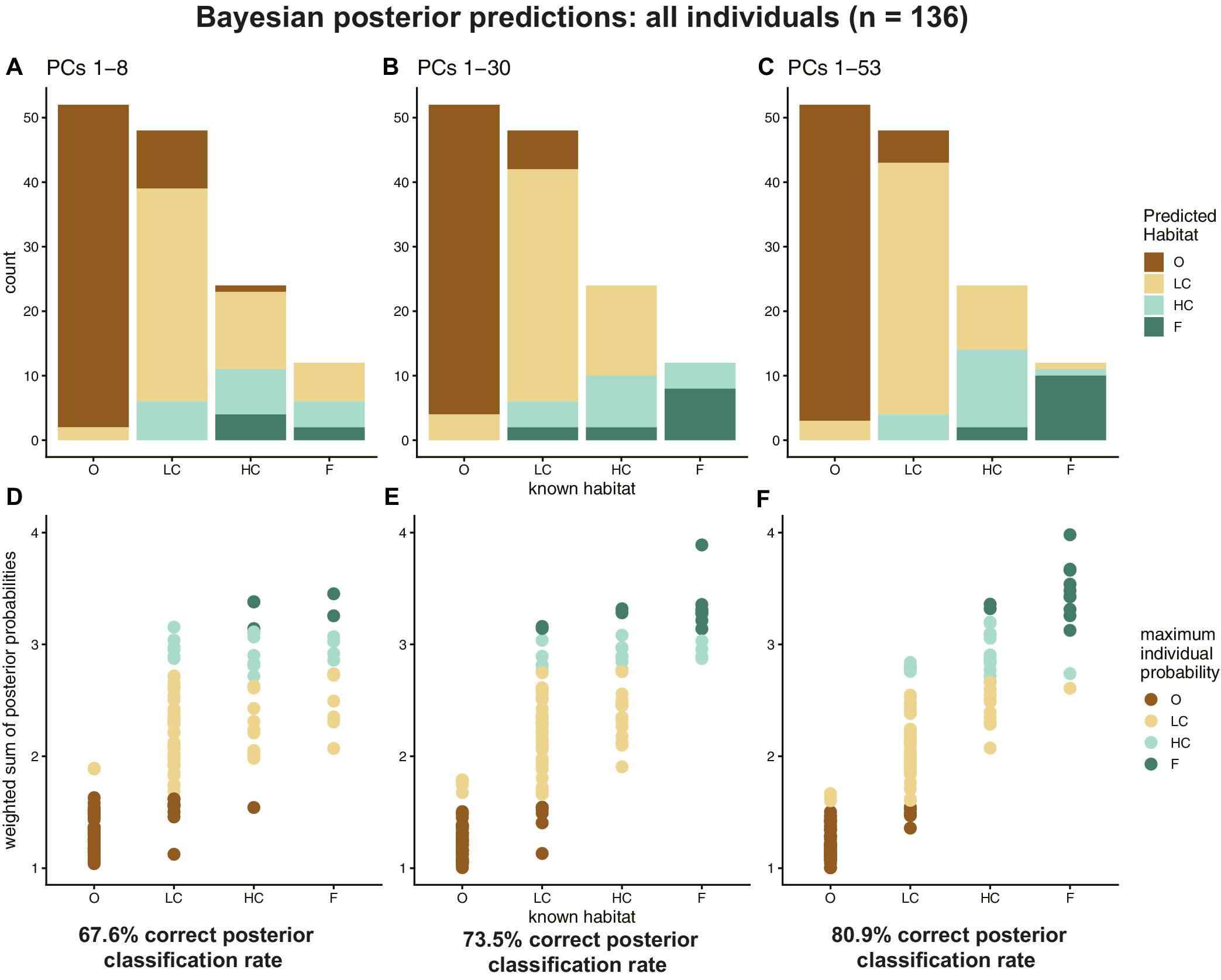
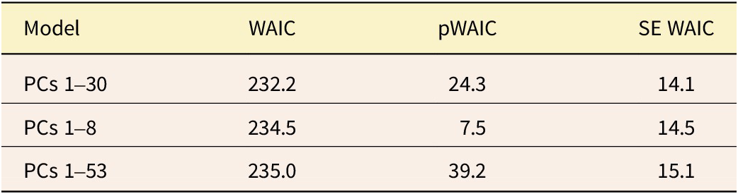

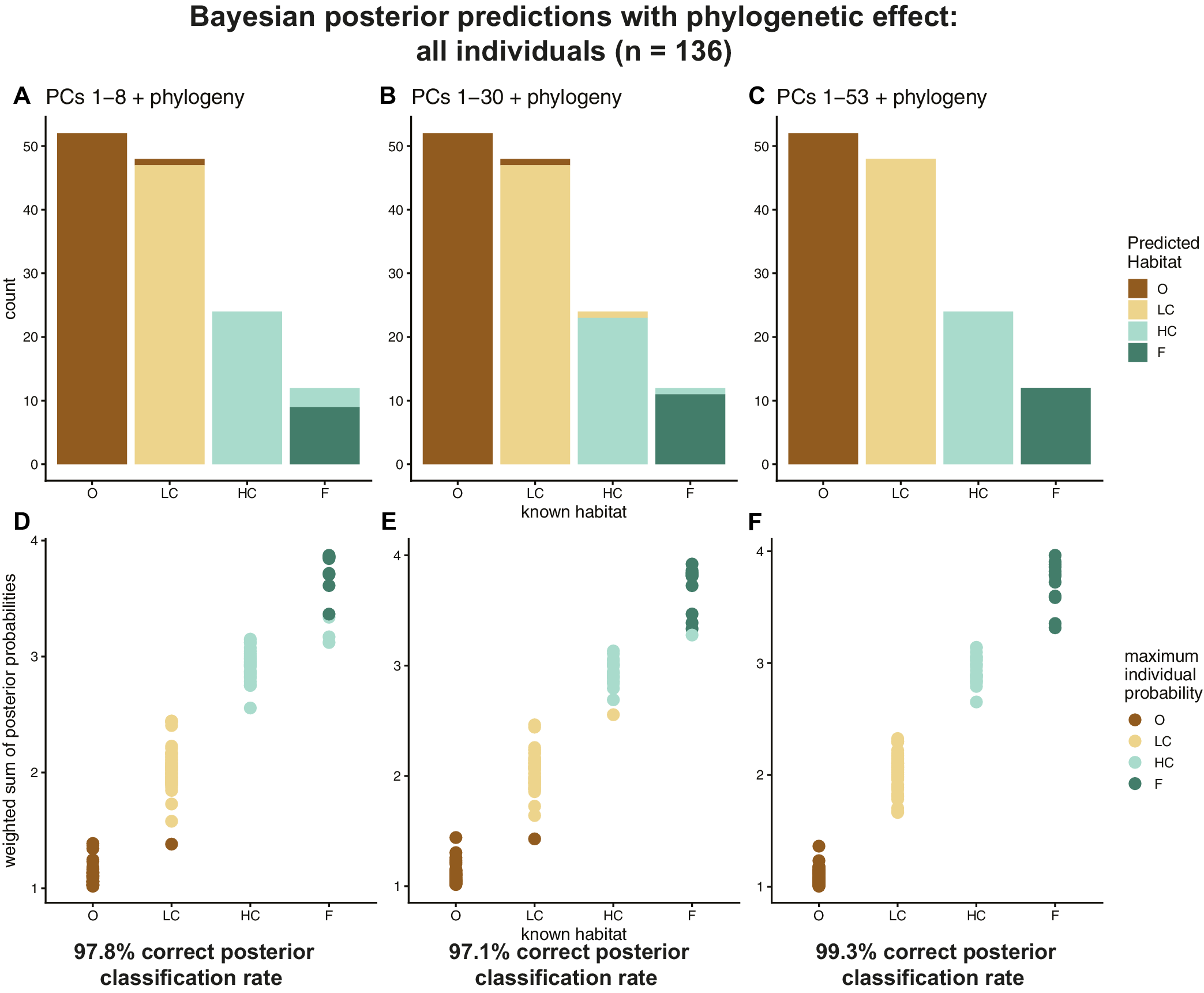
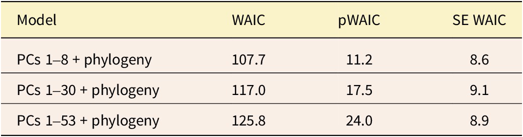
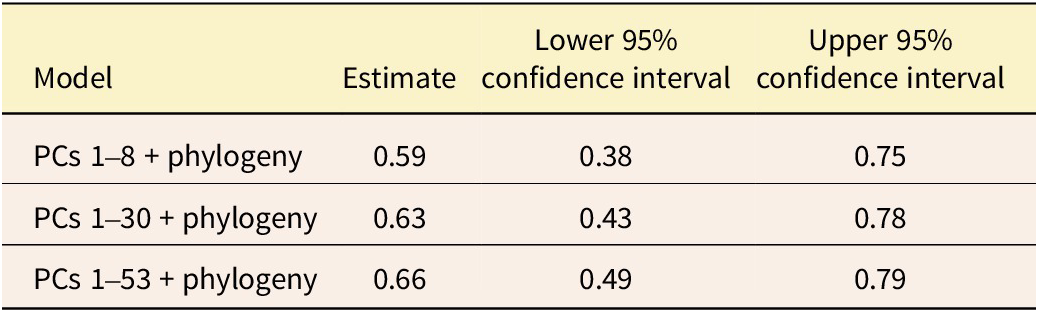
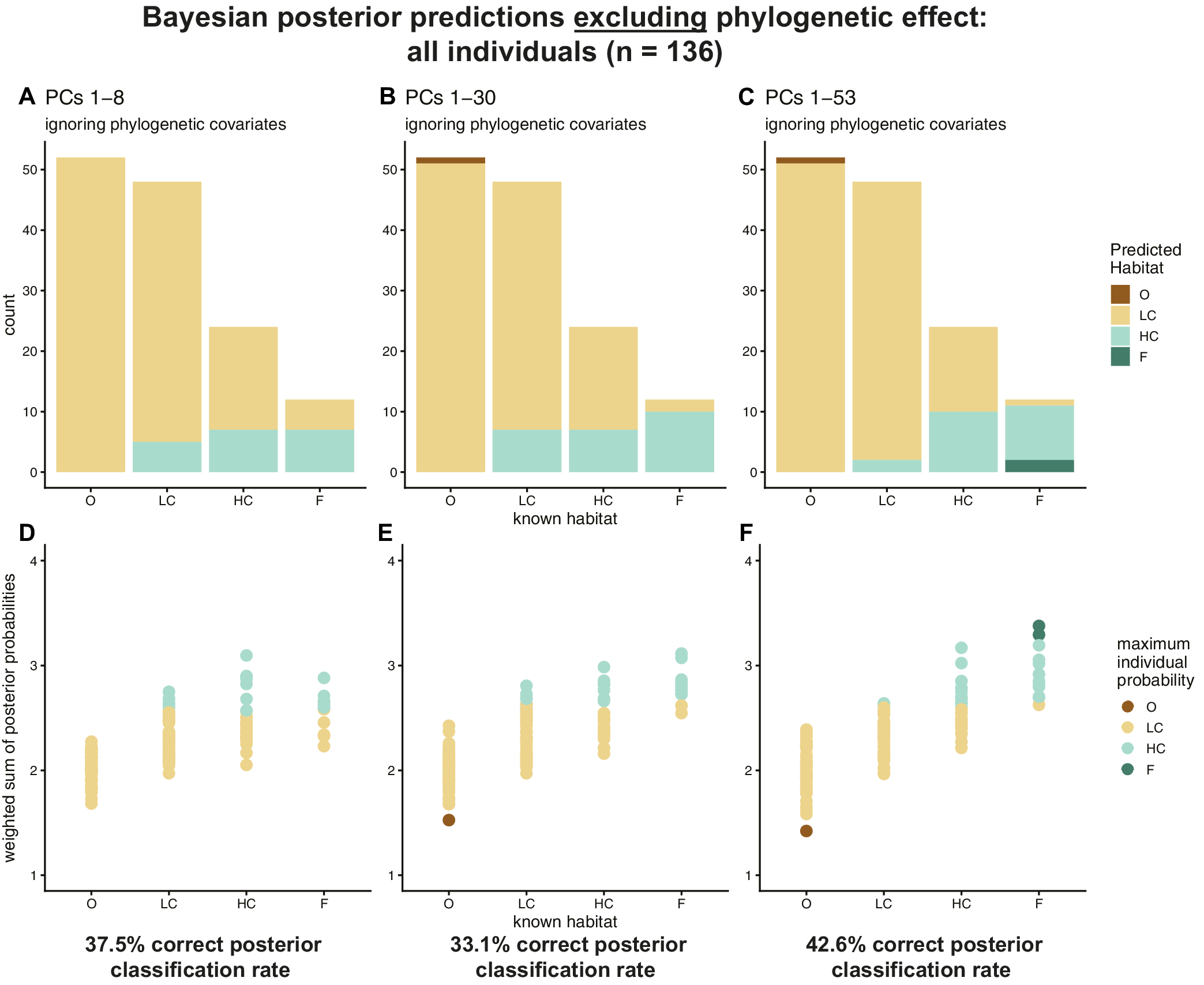
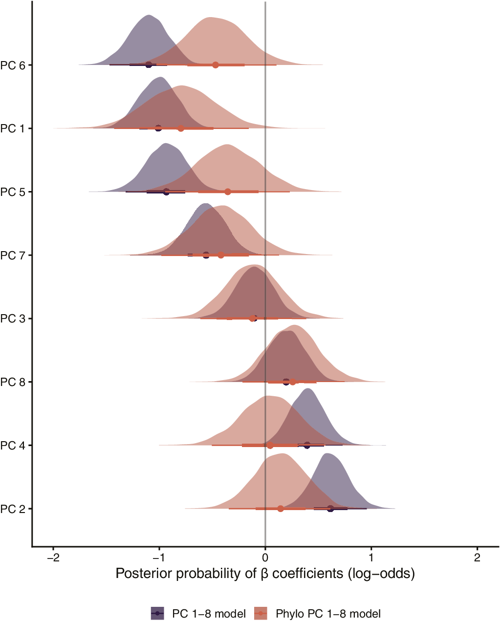
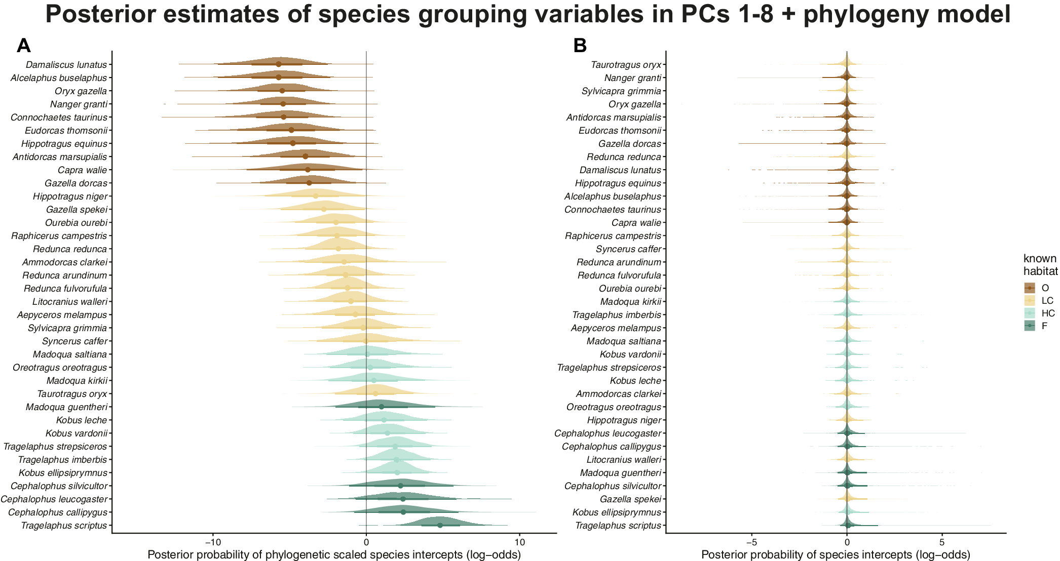


 Open access

