2. NOTATION

For any function g, let g^(m)(x) = (d^m/dx^m)g(x) denote its mth derivative. Let φ(x), φ_σ(x) = σ⁻¹φ(x/σ), and φ_σ^(m)(x) = σ^−1−mφ^(m)(x/σ) denote the standard normal density, the scaled normal density, and its mth derivative, respectively.

We call K(x) a symmetric kernel function if K(x) = K(−x) and ∫_R K(x) dx = 1. Following Müller (1984), we say that K is s-smooth if K^(s−1) is absolutely continuous on R. If the kernel has bounded support, this requires that the (s − 1)th derivative equals zero at the boundaries.

For integer r ≥ 1, a kernel function K is of order 2r if

for all k < 2r yet

. In particular, a kernel is second-order if

.

Pochhammer's symbol is denoted by

A useful result is Legendre's duplication formula:

We will be making extensive use of special functions, for which a useful reference is Magnus, Oberhettinger, and Soni (1966). Many can be represented as generalized hypergeometric functions

For a review of the latter see Abadir (1999). In particular, for integer m ≥ 0, our results will make use of the Gegenbauer polynomials

and the spherical Bessel function

The Gegenbauer polynomials have several hypergeometric representations, including

See Magnus et al. (1966, p. 220).

3. SMOOTH POLYNOMIAL KERNELS

Using a random sample with n real observations X₁,…,X_n drawn independently from a distribution with density f (x), the nonparametric Rosenblatt kernel estimator of f (x) is

where K is a kernel function and h is a bandwidth. The MISE of f_n is

For the moment, restrict attention to s-smooth, second-order kernels with bounded support. Müller (1984) and Granovsky and Müller (1991) found that the MISE of f_n^(s) is minimized by setting K to equal

This class includes the uniform (s = 0), Epanechnikov (s = 1), biweight (s = 2), and triweight (s = 3). Furthermore, as s diverges, the optimal smooth kernel approaches the Gaussian kernel, as

Now consider the more general case of s-smooth bounded-support kernels of order 2r. Müller (1984) and Granovsky and Müller (1991) found that the MISE of f_n^(s) is minimized by using a polynomial kernel of order s + r − 1 in x². We now present several alternative representations for this kernel.

THEOREM 1. Müller's s-smooth, 2rth-order kernel on [−1,1] is

where

Furthermore

Equation (8) gives an explicit formula for the kernel, whereas (9)–(11) give alternatives. For numerical computation, the formula (7)–(8) is numerically reliable.

Granovsky and Müller (1991) examined the limit as s → ∞. They showed that

Here G_2r are the higher order Gaussian kernels of Wand and Schucany (1990) and Marron and Wand (1992).

We now show that as the order 2r increases, both classes of kernels approach the infinite-order Dirichlet kernel D(x) = sin(x)/(πx).

THEOREM 2.

THEOREM 3.

4. CHARACTERISTIC FUNCTION AND ROUGHNESS

For any function g, let

denote the characteristic function of g(x). For example, the characteristic function of the normal density is

.

For the higher order Gaussian kernels, the characteristic function

is given by Wand and Schucany (1990, p. 200). However, the characteristic function has not been calculated previously for the smooth polynomial kernels M_2r,s. We now show that they consist of linear combinations of spherical Bessel functions as defined in (4).

THEOREM 4.

THEOREM 5.

where

For computational purposes, when t is large, the series (4) can be numerically unstable, in which case it is preferable to compute j_m(t) using the recurrence

with the initial conditions

Combining this with Parseval's equality, we can use (15) to calculate the roughness of M_2r,s.

THEOREM 6.

Politis and Romano (1999) introduced a class of infinite-order “general flat-top kernels” that have flat characteristic functions at the origin. Their preferred kernel is

which has the trapezoidal characteristic function

where (t)⁺ = max(t,0). We thus call λ₂(t) the trapezoid kernel. It is easy to calculate that R(λ₂) = 4/(3π).

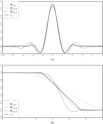
Figure 1a displays the four kernels M_4,8, M_10,8, M_20,8, and λ₂. The kernels have been rescaled and normalized so that all have equal roughness. The basic shapes of the kernels are similar, with the waviness of the kernels increasing in kernel order. The second panel displays the characteristic functions of the same kernels (again normalized to have equal roughness). Here it is easier to see the contrasts. As the kernel order increases, the characteristic functions are increasingly flat at the origin, with the high-order polynomial characteristic function developing a significant negative lobe.

(a) Polynomial and Trapezoid Kernel Functions. (b) Polynomial and Trapezoid Characteristic Functions.

5. EXACT MISE

The exact MISE of the kernel density estimator f_n can be written as

where

with

denoting the characteristic functions of K and f. Equation (19) is shown, for example, in equation (3.1) of Chiu (1991). We write I₀(h,K,f) = I₀(f) because it is independent of K and h.

Marron and Wand (1992) proposed a test set of mixture-normal density functions for which (19) is feasible to calculate. The Marron–Wand densities take the form

The characteristic function of (21) is

with square

where σ_ik² = σ_i² + σ_k² and μ_ik = μ_i − μ_k. We follow Marron and Wand and restrict attention to this class of density functions for our calculation of exact MISE.

From (22) and equation (A.7) in the Appendix, or Theorem 2.1 of Marron and Wand (1992), we find that

. To calculate MISE_n(h,K,f) we also need the integrals I₁(h,K,f) and I₂(h,K,f), which may be calculated by numerical or analytic integration. Although we use numerical integration to calculate MISE in the next section we use analytic integration to verify their accuracy.

Our first result is the integrals for the smooth polynomial kernels.

THEOREM 7. For the mixture-normal densities (21),

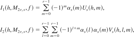
where α_s(m) are defined in (16), and

Our second result is the integrals for the trapezoid and Dirichlet kernels. This extends the work of Davis (1981), who made similar calculations for D when f = φ.

THEOREM 8. For the mixture-normal densities (21),

where

is the incomplete gamma function.

Theorems 7 and 8 express the integrals I₁(h,K,f) and I₂(h,K,f) as convergent infinite series. Methods to numerically evaluate infinite series and other special functions are discussed in detail in Zhang and Jin (1996). As they discuss, numerical evaluation of infinite series can fail as a result of accumulated round-off error when there are alternating signs, which occurs in our expressions. To investigate their accuracy, we numerically compared the expressions in Theorems 7 and 8 with numerical integration for the Marron–Wand densities. We used Gauss–Legendre quadrature with 8,000 grid points over [0,T] where T was selected so that the numerical integral of

was within 0.01% of the exact value

. The results were plotted against h. (See Hansen, 2003.) We found that in some cases the terms in the series expansions grow sufficiently large such that the numerical results are unreliable. This occurred for the polynomial kernels for large h, r, and/or s and also for the trapezoid kernel for very small h in a few cases. We concluded that numerical integration was more reliable for evaluation of I₁(h,K,f) and I₂(h,K,f) for these kernels.

6. ANALYSIS OF MISE

For each kernel we computed MISE_n(h,K,f) on a grid of 3,000 values of h over the region [0,3h*], where h* is the Silverman rule-of-thumb bandwidth for a sample size of 50. Plots of MISE_n(h,K,f) against h for each model and kernel indicated that this region appeared to contain the global minimum for all cases. (See Hansen, 2003.) For given K and f the optimal finite-sample MISE is

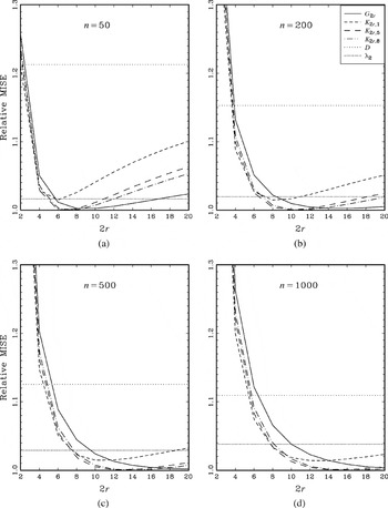
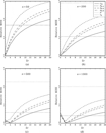
For the kernel classes G_2r and M_2r,s, MISE_n(K,f) was plotted as a function of r. Figures 2 and 3 display these plots for the Marron–Wand densities 1 (the Gaussian density) and 3 (strongly skewed density). These densities are shown here because are they are extreme cases regarding the gain or loss from the use of higher order kernels. Plots for other densities can be seen in Hansen (2003). Plotted are the MISE for the Gaussian kernels G_2r and the smooth polynomial kernels M_2r,1, M_2r,5, and M_2r,8, for 2r = 2,…,20, and for the sample sizes of n = 50, 200, 500, and 1,000. The dotted flat lines are the MISE of D and λ₂, which are independent of r. For each plot, the MISE_n(K,f) is normalized relative to min_K MISE_n(K,f).

MISE, Density 1.

MISE, Density 3.

First examine the flat-top kernels D and λ₂. In nearly all cases, the trapezoid kernel λ₂ does much better than the Dirichlet kernel D, and in most cases λ₂ performs quite well relative to other kernel choices. However, it never has as low MISE as the best Gaussian or polynomial kernel.

Second, compare the smooth polynomial kernels M_2r,s across the smoothness index s. We observe that increasing the smoothness order typically improves the MISE, but the difference diminishes in larger samples. Indeed, for very large samples (not shown), the best MISE is for small s, but the gain is minimal. There also appears to be little gain achieved by increasing s above s = 8 (again not shown), so setting s = 8 emerges as a practical recommendation.

Third, compare the MISE of the smooth polynomial kernel M_2r,8 and the Gaussian kernel G_2r. In most cases the difference in MISE is quite small, with the Gaussian kernels achieving lower MISE in small samples and the reverse in large samples.

Examining the plots of MISE_n(K,f), it is clear that there is no uniformly optimal choice of kernel K (including kernel order) across sample sizes n and densities f. For any given f there may be a best choice of kernel among those we consider, but this choice will vary across f. A data-dependent method such as cross-validation can possibly be used to select kernel order, which might enable estimation to adapt to the unknown density f. This is a difficult problem, however, and is not pursued further in this paper.

7. MINIMAX REGRET KERNELS

Let

denote a class of kernels, such as the Gaussian class {G_2r; r ≥ 1} or the polynomial class {M_2r,s; r ≥ 1;s ≥ 1}. The problem raised at the end of the previous section is how to select a kernel

when it is known that the finite-sample optimal choice varies with the true underlying density f. This section proposes a pragmatic solution based on minimax regret, a concept in statistical decision theory dating back to Savage (1951).

For any density f and sample size n, there is a best possible kernel choice that can be defined as

Note that we implicitly define our loss function as ln MISE_n*(K,f) to eliminate scale effects. The regret associated with the use of an arbitrary kernel K is

the percentage deviation of the realized MISE from the optimal value.

For a compact class of density functions

the maximal regret associated with K is the maximum over

The minimax regret rule is to pick K to minimize the maximum regret

with the associated minimized regret

Note that whereas the small-sample optimal kernel K_n(f) depends on the unknown density f in addition to n, the minimax regret kernel K_n* only depends on the sample size n. The kernel K_n* guarantees that if the true density f belongs to

, the percentage deviation of the MISE from the optimum is bounded by Regret_n*.

For the density class

we use the Marron–Wand mixture-normal class (21) with q = 2:

Many of the Marron–Wand test densities are in this class, and two normal components are sufficient to generate most density shapes of interest. Because the regret criterion is invariant to location and scale, we select μ₂ and σ₂ so that EX = 0 and Var(X) = 1, so the density class is fully described by the remaining parameters (w,μ₁,σ₁). We use a grid over these parameters, varying each in increments of 0.1 over all feasible values. This results in a density class with 1,887 elements.

Setting

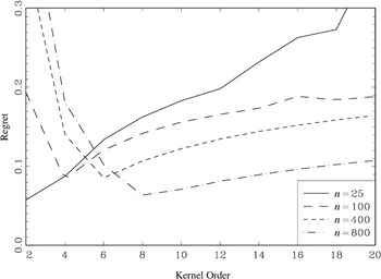
to equal the Gaussian kernel class G_2r, Figure 4 plots Regret_n(G_2r) as a function of 2r for n = 25, 100, 400, and 800. The minimax regret solution r_n* locates its lowest value for any curve. We can see that this solution r_n* varies from 2 to 8 for the four sample sizes.

Regret of Gaussian Kernels.

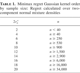
We calculated the minimax regret r_n* for the Gaussian kernels G_2r as a function of sample size, and we present the findings in Table 1. The optimal kernel order r_n* is strictly increasing with n. The magnitudes may be surprising to many readers, as the minimax kernel orders are higher than typically used in practice.

Minimax regret Gaussian kernel order by sample size: Regret calculated over two-component normal mixture densities

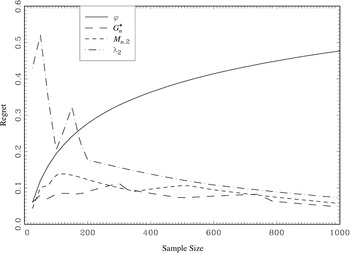
Let G_n* denote the Gaussian higher order kernel with r = r_n*, and similarly M_n,s*. These are feasible kernel choices as they vary only with sample size. We now compare the regret of the feasible kernel choices φ, G_n*, M_n,2*, and λ₂. Figure 5 plots Regret_n* for these kernels as a function of n where the general kernel class includes G_2r, M_2r,2, and λ₂. We see that the standard normal kernel φ has regret that is increasing in n and is clearly dominated by the other choices except when the sample size is very small. The trapezoid kernel λ₂ has high regret for small samples but has comparable regret with the optimal Gaussian and polynomial kernels for large samples. The optimal Gaussian and polynomial kernels have similar regret for most sample sizes, with that for G_n* slightly lower. Because G_n* is somewhat easier to manipulate numerically, it is our recommendation for empirical practice. A sensible alternative choice is the trapezoidal kernel λ₂, as long as n ≥ 500 (its regret is bounded below 12% for such samples).

Regret across Kernel Classes.

Finally, from Figure 5 we find that the regret of G_n* is uniformly bounded below 12%. This means that this kernel choice guarantees that regardless of f (in the class of two-component mixture-normal distributions) the MISE_n*(G_n*,f) cannot differ from the optimal MISE_n*(K_n(f),f) by more than 12%.