2.1. Computational domain

A schematic diagram of the present computational domain is shown in figure 1(a). The inflow is a spatially developing 2-D ZPG TBL over a flat plate (this point will be detailed in § 2.3). After the inlet, the present TBL develops under the ZPG in the region $0 \le x \le {L_{{W_S}1}}$. The flow is then subjected to a sudden imposition of the surface spanwise velocity ${W_S}$ in the region ${L_{{W_S}1}} \le x \le {L_{{W_S}2}}$ (this latter region is referred to as the ‘3DTBL region’ in this paper). The streamwise extent of imposing ${W_S}$, i.e. ${L_{x,{W_S}}} = {L_{{W_S}2}} - {L_{{W_S}1}}$, will be examined in § 3.1 in light of Lohmann's (Reference Lohmann1976) condition on the near-equilibrium 3DTBL state. Note that different values of ${L_{x,{W_S}}}$ are used for $R{e_{{\theta _0}}} = 300$ and for $R{e_{{\theta _0}}} = 600$ and 900 (see table 1) since a longer ${L_{x,{W_S}}}$ is required for a lower ${L_{x,{W_S}}}$ to obtain a near-plateau in both the streamwise and spanwise skin friction coefficients (see §§ 3–5). At x = ${L_{{W_S}2}}$, ${W_S}$ is turned off. There is again a sudden change of the surface condition there. The present flow recovers to a ZPG TBL in the region ${L_{{W_S}2}} \le x \le {L_x}$ (referred to as the ‘recovery region’ in this paper).

Table 1.

Domain size, grid points, spatial resolution and sampling time period. Note that $\delta_{out}$ denotes the outlet 99% boundary layer thickness.

2.2. Numerical methodology

Numerical methodology is briefly as follows. The current DNS code has been developed based on a DNS code for a TBL with separation and reattachment by Abe (Reference Abe2017). A fractional step method is used with semi-implicit time advancement. The Crank–Nicolson method is used for the viscous terms in the y direction, and the third-order Runge–Kutta method is used for the other terms. A finite difference method is used as a spatial discretization. A fourth-order central scheme (Morinishi et al. Reference Morinishi, Lund, Vasilyev and Moin1998) is used in the x and z directions, whilst a second-order central scheme is used in the y direction.

As for the boundary condition for W at the wall (y = 0), a slip boundary condition (i.e. $W = {W_S}$) is used in the 3DTBL region (i.e. ${L_{{W_S}1}} \le x \le {L_{{W_S}2}}$), whereas a no-slip boundary condition is used in the other x locations. For U and V at the wall, a no-slip boundary condition is used across the x stations. On the other hand, we impose the following boundary conditions at the upper boundary:

(2.1a–c)\begin{equation}\frac{{\partial U}}{{\partial y}} = 0,\quad V = {U_0}\overline {\frac{{\partial {\delta _2}}}{{\partial x}}} ,\quad \frac{{\partial W}}{{\partial y}} = 0,\end{equation}

which are the same ones as for a ZPG TBL by Lund, Wu & Squires (Reference Lund, Wu and Squires1998). Note that (2.1b) (i.e. the wall-normal velocity at the upper boundary) consists of the product of ${U_0}$ and $\partial {\delta _2}/\partial x$ (i.e. the gradient of the displacement thickness at each x station) averaged over the x direction. In the z direction, a periodic boundary condition is used; the spatial averaging for mean and turbulence statistics has been made for this direction. For the outlet, a convective boundary condition is used.

2.3. Inflow 2DTBL simulation

The present inflow is a spatially developing 2-D ZPG TBL over a flat plate, which is generated by the rescaling–recycling method (Lund et al. Reference Lund, Wu and Squires1998) with a spanwise constant shift (Spalart, Strelets & Travin Reference Spalart, Strelets and Travin2006). This simulation has been time-advanced simultaneously with the shear-driven 3DTBL DNS, i.e. the ZPG data at a target $R{e_\theta }$ are provided as the inlet data of a shear-driven 3DTBL DNS. In the inflow simulations, the domain size used for $R{e_{{\theta _0}}} = 300$ and 600 is L_x × L_y × L_z = 400θ ₀ × 80θ ₀ × 160θ ₀ where the inlet momentum thickness Reynolds number is set to 300 and 600. On the other hand, the domain size used for $R{e_{{\theta _0}}} = 900$ is L_x × L_y × L_z = 1200θ ₀ × 240θ ₀ × 480θ ₀ where the inlet momentum thickness Reynolds number is set to 300. Referring to the seminal DNS by Kong, Choi & Lee (Reference Kong, Choi and Lee2000), the recycling location has been set to approximately 100θ ₀ for all the inflow simulations. The validation of the inflow simulation has been presented in Abe (Reference Abe2017). Overall agreement with the existing DNS in a ZPG TBL (Spalart Reference Spalart1988; Simens et al. Reference Simens, Jimenez, Hoyas and Mizuno2009; Wu & Moin Reference Wu and Moin2009; Schlatter & Örlü Reference Schlatter and Örlü2010) is satisfactory (see § 2 of Abe Reference Abe2017). In the following sections, statistics and turbulence structures for a 2DTBL will be compared with those for a 3DTBL.

2.4. Flow parameters for the shear-driven 3DTBL DNS

The computational domain size (L_x × L_y × L_z), number of grid points (N_x × N_y × N_z), spatial resolution at the inlet ($\Delta {x_0},\Delta {y_0},\Delta {z_0}$) and sampling time period (T) for the shear-driven 3DTBL simulations are given in table 1. The present streamwise domain size (i.e. ${L_x}/{\theta _0} = 400$ or, equivalently, $48{\delta _0}$) is comparable with ${L_x}/{\theta _0} \approx 350$ (note that this latter domain size does not involve a buffer region of a fringe) of Kannepalli & Piomelli (Reference Kannepalli and Piomelli2000), whereas the spanwise domain size (i.e. ${L_z}/{\theta _0} = 160$ or, equivalently, $19{\delta _0}$) is a factor of 4 larger than in Kannepalli & Piomelli (Reference Kannepalli and Piomelli2000) – a small spanwise domain (i.e. ${L_z}/{\theta _0} \approx 40$ or, equivalently, 5δ ₀) is used in their work. Once the velocity field reaches the fully developed and statistically steady state (i.e. time-independent profiles of the skin friction coefficients), the Navier–Stokes equations are integrated further in time to obtain mean flow and turbulence statistics (we have also checked one-point statistics for the first sampling time period (0–T/2) and those for the second sampling time period (T/2–T) and confirmed that the difference is negligibly small).

In the present study, we examine the effects of cross-flow and Reynolds number in a shear-driven 3DTBL. The former effect is examined for $R{e_{{\theta _0}}} = 300$ with varying ${W_S}/{U_0}$ (= 0, 0.1, 0.5, 1, 1.5 and 2). On the other hand, the latter effect is investigated for three values of $R{e_{{\theta _0}}}$ (= 300, 600 and 900) with two different magnitudes of ${W_S}/{U_0}$ (= 1 and 2). The three values of the inlet momentum thickness Reynolds number, $R{e_{{\theta _0}}} = 300$, 600 and 900, correspond to those of the friction Reynolds number, ${Re _{{\tau _0}}} \equiv {U_{{\tau _0}}}{\delta _{{{99}_0}}}/\nu = 140$, 250 and 350, respectively (here ${U_{{\tau _0}}}$ and ${\delta _{{{99}_0}}}$ denote the inlet friction velocity and 99 % boundary layer thickness, respectively). In the present flow, the momentum thickness Reynolds number increases with increasing x (see figure 13a). Also shown in table 2 is the momentum thickness Reynolds number $R{e_\theta }$ in the 3DTBL ($x/{\theta _0} = 175$) and recovery ($x/{\theta _0} = 300$) regions. At $x/{\theta _0} = 175$, the largest $R{e_\theta }$ (= 1255) is attained for $R{e_{{\theta _0}}} = 900$ with ${W_S}/{U_0} = 2$, the latter magnitude of $R{e_\theta }$ being close to that (i.e. $R{e_\theta } = 1450$) in the PIV measurement of Kiesow & Plesniak (Reference Kiesow and Plesniak2003). In § 5, the effects of Reynolds number will be discussed mainly at these two stations.

Table 2.

The momentum thickness Reynolds number $R{e_\theta }$ in the 3DTBL ($x/{\theta _0} = 175$) and recovery ($x/{\theta _0} = 300$) regions. The values tabulated have been obtained with ${L_{x,{W_S}}} = 100{\theta _0}$.

3.1. Value of ${L_{x,{W_S}}}$ and approach to the collateral state

We first discuss the value of ${L_{x,{W_S}}}$ in the current 3DTBL simulation. Given that Lohmann (Reference Lohmann1976) reported in his spinning cylinder experiment that the transverse mean velocity and wall shear-stress component attain an asymptotic state in the streamwise distance of approximately 10δ ₀, we here examine three cases with different values of ${L_{x,{W_S}}}$, i.e. ${L_{x,{W_S}}} = 100{\theta _0}$, 200θ ₀ and 300θ ₀ (or, equivalently, 12δ ₀, 24δ ₀ and 36δ ₀), where ${L_{{W_S}1}} = 100{\theta _0}$ and ${L_{{W_S}2}} = 200{\theta _0}$, 300θ ₀ and 400θ ₀.

Figure 2(a,b) shows the distributions of the streamwise and spanwise skin friction coefficients, ${C_{f,x}} \equiv {\tau _{w,x}}/\textrm{(}\rho U_0^2/2)$ and ${C_{f,z}} \equiv {\tau _{w,z}}/\textrm{(}\rho U_0^2/2)$, as a function of $x/{\theta _0}$. Note that ${\tau _{w,x}} \equiv \mu \textrm{(}\partial \bar{U}/\partial y){\textrm{|}_w}$ and ${\tau _{w,z}} \equiv \mu \textrm{(}\partial \textrm{(}\bar{W} - {W_S})/\partial y){|_w}$, where $\mu = \nu /\rho $. After imposing ${W_S}$, ${C_{f,x}}$ decreases abruptly, due to a non-equilibrium effect (disorganization of the near-wall turbulence). This drop would not appear in a laminar flow since the independence principle, traditionally proposed for swept wings, holds exactly there (this was pointed out by Dr P. R. Spalart, private communication 2019) (see also McLean Reference McLean2013; Coleman et al. Reference Coleman, Rumsey and Spalart2019). After this drop, ${C_{f,x}}$ and ${C_{f,z}}$ increase significantly with increasing x. We then see a near-plateau in the region $x \ge 250{\theta _0}$ and $x \ge 200{\theta _0}$ for ${C_{f,x}}$ and ${C_{f,z}}$, respectively. The angle of the mean wall shear stress, i.e. ${\tan ^{ - 1}}({C_{f,z}}/{C_{f,x}})$ (figure 2c), however, does not approach −45°, the latter angle being expected when the collateral state is established. Also, the magnitude of ${C_{f,x}}$ in the collateral boundary layer is estimated to be a factor of 2^1/2 (i.e. $2\cos ( - 45^\circ )$) larger than that in a 2DTBL since, in the collateral boundary layer, $U_0^2$ is replaced by $U_0^2 + W_S^2$. Figure 2(a) highlights that the approach to a normal 2DTBL is slow for ${C_{f,x}}$. An estimate of ${L_{x,{W_S}}}$ from figure 2 for reaching the collateral state for $R{e_{{\theta _0}}} = 300$ would be approximately 1000θ ₀ (or, equivalently, approximately 100δ ₀). This condition is a factor of 10 larger than that of Lohmann (Reference Lohmann1976).

Figure 2.

Distributions of (a) ${C_{f,x}}$, (b) ${C_{f,z}}$ and (c) ${\tan ^{ - 1}}({C_{f,z}}/{C_{f,x}})$ as functions of $x/{\theta _0}$ for $R{e_{{\theta _0}}} = 300$ with ${W_S}/{U_0} = 1$. The data shown have been obtained with ${L_{x,{W_S}}} = 100{\theta _0}$, 200θ ₀ and 300θ ₀.

Figure 3 shows the distribution of the mean velocity magnitude normalized by the friction velocity, $Q_r^{+}( = {Q_r}/{U_\tau })$, at a downstream station $x/{\theta _0} = 350$ for the case with ${L_{x,{W_S}}} = 300{\theta _0}$. Note that the friction velocity in a non-zero cross-flow ($\overline W \ne 0$) region (i.e. ${L_{{W_S}1}} \le x \le {L_x}$) is obtained such that

(3.1)\begin{equation}{U_\tau } \equiv ([\tau _{w,x}^2 + \tau _{w,z}^2]^{1/2}/\rho)^{1/2}.\end{equation}

While ${C_{f,x}}$ exhibits a near-plateau at this station, the agreement between ${Q_r}/{U_\tau }$ and $\overline U /{U_{\tau,x}}$ is confined to the near-wall region, i.e. there is a departure from the collateral state (i.e. (1.5) and (1.6)) away from the wall. In particular, the magnitude of $Q_r/U_\tau$ is smaller than that of $\overline{U}/ U_{\tau ,x}$ obtained from the 2DTBL simulation. On the other hand, the distribution of $\overline W /{U_{\tau ,z}}$ follows the collateral relation (1.4) reasonably well (note that ${U_{\tau,z}} \equiv {\left( {{\tau _{w,z}}/\rho } \right)^{1/2}} $). This indicates that the mean spanwise velocity develops faster than the mean streamwise velocity. This latter behaviour will also be discussed further in § 5.

Figure 3.

Distributions of the normalized mean velocity magnitude $Q_r^{}$ for $R{e_{{\theta _0}}} = 300$ with ${W_S}/{U_0} = 1$ at a downstream station of a 3DTBL ($x/{\theta _0} = 350$). The data shown have been obtained with ${L_{x,{W_S}}} = 300{\theta _0}$.

3.2. Relationship between the streamwise velocity deficit and inviscid skewing

As was mentioned in the introduction, there is close association between the mean streamwise velocity deficit $\partial \overline U /\partial x \lt 0$ and inviscid skewing $\partial \overline W /\partial x$ (see (1.5) and (1.6)).

Figure 4 shows the contours in the x–y plane of non-dimensionalized ${\overline \varOmega _x}$, $\partial \overline U /\partial x$ and $\partial \overline W /\partial x$. In the region where ${W_S}$ is imposed, ${\overline \varOmega _x}$ (i.e. mean streamwise vorticity) increasingly diffuses towards the outer region until $x/{\theta _0} = 250$. In the region $x/{\theta _0} \le 250$, there is indeed a close relationship between inviscid skewing ($\partial \overline W /\partial x \gt 0$) and mean streamwise velocity deficit ($\partial \overline U /\partial x \lt 0$). After $x/{\theta _0} = 250$, the development of ${{\overline \varOmega } _x}$ becomes increasingly small as we move downstream for the two cases using ${L_{x,{W_S}}} = 200{\theta _0}$ and 300θ ₀, where the regions of $\partial \overline U /\partial x \lt 0$ and $\partial \overline W /\partial x \gt 0$ become small, and ${C_{f,x}}$ exhibits near-constancy. Note that, when ${L_{x,{W_S}}} = 100{\theta _0}$ and 200θ ₀, there are two transitions from a 2DTBL to a 3DTBL and from a 3DTBL to a 2DTBL. Even in these transitions, we do not observe mean streamwise circulation in the 3DTBL region, but see a streamwise development of the mean streamwise vorticity (see figure 4).

Figure 4.

Contours in the x–y plane of the normalized ${\overline \varOmega _x}$, $\partial \overline U /\partial x$ and $\partial \overline W /\partial x$ for $R{e_{{\theta _0}}} = 300$ with ${W_S}/{U_0} = 1$ using ${L_{x,{W_S}}} = 100{\theta _0}$ (a–c), 200θ ₀ (d–f) and 300θ ₀ (g–i): (a,d,g) $({\theta _0}/{U_0}){\overline \varOmega _x}$; (b,e,h) $({\theta _0}/{U_0})(\partial \overline U /\partial x)$; and (c,f,i) $({\theta _0}/{U_0})(\partial \overline W /\partial x)$.

The degree of skewing (turning) of the present 3DTBL can readily be confirmed in mean velocity hodographs (figure 5a). At a downstream station of a 3DTBL where ${C_{f,x}}$ starts to exhibit a plateau (i.e. $x = 250{\theta _0}$), the profiles (the red lines) follow the linear solid line with the slope of −1.25. The value of arctan (−1.25) is approximately $- 51\mathrm{^\circ }$, which agrees well with the direction of the surface shear stress, i.e. ${\tan ^{ - 1}}({C_{f,z}}/{C_{f,x}})$ (see figure 2c). This result indicates that the mean flow has a constant flow angle near the wall. It is well recognized that, for a small turning angle, the spanwise velocity gradient angle is often approximated by the Squire–Winter–Hawthorne equation, i.e.

(3.2)\begin{equation}\frac{\partial }{{\partial x}}\left( {\frac{{\partial \overline{W}/\partial y}}{{\partial \overline{U}/\partial y}}} \right) = \frac{\partial }{{\partial x}}\left( {\frac{{\overline{W}}}{{\overline{U}}}} \right)\end{equation}

(see Bradshaw Reference Bradshaw1987). Note that the minus sign is omitted on the right-hand side of (3.2) since $\partial \overline W /\partial y \lt 0$ in the present flow. Figure 5(a,b) indicates that relation (3.2) holds reasonably at a downstream station of a 3DTBL (see the red lines representing the profiles at $x = 250{\theta _0}$). The same is, however, not true for the Reynolds shear stress, i.e. there is a larger departure from the −1.25 slope for the Reynolds stress hodograph (figure 5c) than for the mean strain-rate one (figure 5b). This underlines that the Reynolds shear stress lags behind the mean strain rate in the 3DTBL region.

Figure 5.

Hodograph plots in the 3DTBL region for $R{e_{{\theta _0}}} = 300$ with ${W_S}/{U_0} = 1$: (a) mean velocity hodograph; (b) mean strain-rate hodograph; and (c) Reynolds shear-stress hodograph. The red lines refer to the data at $x/{\theta _0} = 250$ where a near-plateau has been established in ${C_{f,x}}$. The data shown have been obtained with ${L_{x,{W_S}}} = 300{\theta _0}$. In (b), normalization is made with $U_0\ \textrm{and}\ \theta_0.$

3.3. Basic statistics in the present non-equilibrium 3DTBL

Here, we explain the basic features of the present non-equilibrium 3DTBL by showing mean velocities and some turbulence statistics for the case using ${L_{x,{W_S}}} = 300{\theta _0}$.

Figure 6 shows the distributions of outer-normalized mean velocities (i.e. $\overline U /{U_0}$ and $\overline W /{U_0}$) and Reynolds shear stresses (i.e. $- \overline {uv} /U_0^2$ and $\overline {vw} /U_0^2$) at several x stations in a 3DTBL region. After imposing ${W_S}$, $\overline W$ (i.e. cross-flow) increasingly develops from the near-wall region to the outer layer (see figure 6b), where the secondary Reynolds shear stress $\overline {vw}$ builds up – this quantity is amplified due to the production term $- \overline {vv} (\partial \overline W /\partial y)$ (the distribution is not shown here) – and the latter magnitude increases as x increases (figure 6d). On the other hand, the magnitude of $\overline U$ is decreased in a 3DTBL region (see figure 6a) where there is reduction in the magnitude of $\overline {uv}$; the decreased $\overline {uv}$ propagates outwards with increasing x (see figure 6c). Lohmann (Reference Lohmann1976) noted that the increase in Reynolds stress causes an increasing velocity deficit to develop in the inner part of a 3DTBL. Kiesow & Plesniak (Reference Kiesow and Plesniak2003) explained that the deficit of $\overline U$ results from an increase in the streamwise wall shear stress. The present results indicate that the decreased magnitude of $\overline U /{U_0}$ is intrinsically associated with inviscid skewing (see figure 4, where the region of $\partial \overline W /\partial x \gt 0$ corresponds well with that of $\partial \overline U /\partial x \lt 0$), consistent with the finding of Coleman et al. (Reference Coleman, Kim and Spalart2000) in their temporally developing DNS for an idealization of pressure-driven TBLs.

Figure 6.

Distributions of normalized $\overline U$, $\overline W$, $\overline {uv}$ and $\overline {vw}$ in the 3DTBL region for $R{e_{{\theta _0}}} = 300$ with ${W_S}/{U_0} = 1$: (a) $\overline U /{U_0}$; (b) $\overline W /{U_0}$; (c) $- \overline {uv} /U_0^2$; and (d) $\overline {vw} /U_0^2$. The red lines refer to the data at $x/{\theta _0} = 250$ where a near-plateau has been established in ${C_{f,x}}$. The data shown have been obtained with ${L_{x,{W_S}}} = 300{\theta _0}$.

At a downstream station of a 3DTBL, the magnitude of $- \overline {uv} /U_0^2$ is smaller than that of $\overline {vw} /U_0^2$ (see figure 6c,d), which is intrinsically associated with the inefficiency in extracting energy from mean flow, as will be discussed in §§ 4.1 and 5.1. The decreased magnitude of $- \overline {uv} /U_0^2$ implies a lag between the Reynolds shear stress and mean strain-rate vectors (see the discussion in § 3.2). Note that the reduced $\overline {uv}$ is not observed in the 3-D channel DNS of Lozano-Durán et al. (Reference Lozano-Durán, Giometto, Park and Moin2020) at a low Reynolds number (i.e. Re_τ = 180), although in both the present and their simulations, ${\overline \varOmega _x}$ propagates from the near-wall region to the outer layer. This difference seems to be that between internal and external flows (i.e. channel and boundary layer) since a channel flow has two walls and is likely to suffer from the effect of insufficient scale separation at low Reynolds number. On the other hand, the present 3DTBL increasingly develops from the near-wall region towards the outer region (this latter region is initially a 2DTBL) by inviscid skewing (i.e. three-dimensionality). The reduced $\overline {uv}$ is thus observed independent of Reynolds number. The reason for the decrease in $\overline {uv}$ will be discussed in § 5.4.

As for the turbulence statistics, there is a sudden decrease in the magnitudes of the turbulent kinetic energy k (figure 7a), the total Reynolds shear stress $\tau \equiv {({\overline {vw} ^2} + {\overline {uv} ^2})^{1/2}}$ (figure 7b) and the energy dissipation rate $\overline \varepsilon \equiv \nu \overline {{u_{i,j}}({u_{i,j}} + {u_{j,i}})}$ (figure 7c) in the region $x/{\theta _0} = 100\sim125$. A similar decrease is found for the temporally developing DNS of Moin et al. (Reference Moin, Shih, Driver and Mansour1990) and Coleman et al. (Reference Coleman, Kim and Le1996), which is attributed to a non-equilibrium effect. After this drop, the near-wall magnitudes of $k/U_0^2$, $\tau /U_0^2$ and $\overline \varepsilon {\delta_{99}}/U_0^3$ increase with x. In particular, $\overline \varepsilon {\delta_{99}}/U_0^3$ exhibits a larger magnitude close to a wall than that for a 2DTBL (figure 7c), qualitatively similar to those observed in the temporally developing DNS of Moin et al. (Reference Moin, Shih, Driver and Mansour1990). At $x/{\theta _0} = 250$ (see the red lines in figure 7), the increase in $k/U_0^2$ and $\tau /U_0^2$ from a 2DTBL is approximately a factor of 2. The latter factor is estimated by considering the collateral boundary layer where $U_0^2$ is replaced by $U_0^2 + W_S^2$. This indicates that the turbulence develops by cross-flow (arising from ${W_S}$) effectively in a 3DTBL, although the Reynolds stress anisotropy is not altered adequately with this short transition length (see figure 6, where the peak magnitude of $- \overline {uv} /U_0^2$ is smaller than that of $\overline {vw} /U_0^2$).

Figure 7.

Distributions of (a) $k/U_0^2$, (b) $\tau /\rho U_0^2$, (c) $\overline \varepsilon {\delta _{99}}/U_0^3$ and (d) ${a_1}$ in the 3DTBL region for $R{e_{{\theta _0}}} = 300$ with ${W_S}/{U_0} = 1$. The red lines refer to the data at $x/{\theta _0} = 250$ where a near-plateau has been established in ${C_{f,x}}$. The data shown have been obtained with ${L_{x,{W_S}}} = 300{\theta _0}$.

Also, it would be instructive to address how the structure parameter ${a_1}$ varies on moving downstream in the present 3DTBL given that significant attention has been paid to this quantity in the earlier experimental and DNS works. Figure 7(d) shows the distributions of the structure parameter ${a_1}$ in terms of $y/{\delta _{99}}$ in the 3DTBL region (note that ${\delta _{99}}$ denotes the 99 % boundary layer thickness). After the initial drop, the magnitude of ${a_1}$ tends to approach that of a 2DTBL at $x/{\theta _0} = 250$ below $y/{\delta _{99}} = 0.2$, consistent with the behaviour of $k/U_0^2$ and $\tau /U_0^2$. The approach to the 2DTBL is also observed in the equilibrium 3DTBL simulations (Spalart Reference Spalart1989; Wu & Squires Reference Wu and Squires1997). There is, however, a decrease in the magnitude of ${a_1}$ away from the wall (figure 7d) owing to the reduction of $\tau$ (figure 7b). Note that the y location at which ${a_1}$ exhibits a decreased magnitude moves outwards with increasing x, whereas for $\overline {uv}$, the decrease is not observed for ${a_1}$ at a low Reynolds number in a 3-D channel DNS of Lozano-Durán et al. (Reference Lozano-Durán, Giometto, Park and Moin2020).

4.1. Skin friction coefficients

Figure 8(a,b) shows the distributions of the streamwise and spanwise skin friction coefficients, ${C_{f,x}}$ and ${C_{f,z}}$, as a function of $x/{\theta _0}$. After imposing ${W_S}$, ${C_{f,x}}$ decreases abruptly in the 3DTBL region (i.e. $100 \le x/{\theta _0} \le 300$) when ${W_S}/{U_0} \ge 0.5$. This is due to a non-equilibrium effect. After this decrease, ${C_{f,x}}$ and ${C_{f,z}}$ increase significantly with increasing ${W_S}$. The rates of increase in ${C_{f,x}}$ and ${C_{f,z}}$ from ${W_S}/{U_0} = 1$ and 2 (i.e. ${\tan ^{ - 1}}({{W_S}/{U_0}} )={-} 45^\circ$ and $- 63^\circ$) are approximately 1.2 and 2.5, respectively, at $x/{\theta _0} \approx 250$, while 1.5 ($= 5\cos ( - 63^\circ )/2\cos ( - 45^\circ )$) and 3.0 ($= 5\sin ( - 63^\circ )/2\sin ( - 45^\circ )$) are estimated from the collateral state. The approach to the collateral state is slower for ${C_{f,x}}$ than for ${C_{f,z}}$, which is intrinsically associated with the inefficiency in extracting energy from mean flow by the Reynolds shear stress $- \overline {uv}$. This point will be discussed below.

Figure 8.

Distributions of (a) ${C_{f,x}}$, (b) ${C_{f,z}}$ and (c) ${C_{f,z\,mixed}}$ as functions of $x/{\theta _0}$ for $R{e_{{\theta _0}}} = 300$ with varying ${W_S}$. The data shown have been obtained with ${L_{x,{W_S}}} = 200{\theta _0}$.

For ${C_{f,z}}$, Kannepalli & Piomelli (Reference Kannepalli and Piomelli2000) proposed a mixed scaling such that

(4.1)\begin{equation}{C_{f,z\,mixed}} = {\tau _{w,z}}/\textrm{(}\rho {U_0}{W_S}/2).\end{equation}

Figure 8(c) demonstrates that this scaling holds reasonably well for ${W_S}/{U_0} \le 1$, but not for ${W_S}/{U_0} \gt 1$ inside the 3DTBL region ($100 \le x/{\theta _0} \le 300$). This is essentially associated with the departure from the half-power law of ${\theta _z}$, as will be discussed in § 5 (see figure 13b). On the other hand, (4.1) holds excellently in the recovery region ($300 \le x/{\theta _0} \le 400$) independent of ${W_S}$. The forcing (i.e. the imposition of ${W_S}$) thus most likely yields the departure from (4.1).

To gain further insight into the behaviour of the skin friction coefficients, we here examine the mean energy balance, by referring to the work of Renard & Deck (Reference Renard and Deck2016) in a 2DTBL, for the streamwise skin friction coefficient ${C_{f,x}}$, i.e.

(4.2)\begin{equation}\begin{array}{ccccc} {C_{f,x}} & =\underbrace{{\dfrac{2}{{U_0^3}}\int_0^\infty {\nu {{\left( {\dfrac{{\partial \overline U }}{{\partial y}}} \right)}^2}} \,\textrm{d}y}}_{{{C_{f,x\,vis}}}} + \underbrace{{\dfrac{2}{{U_0^3}}\int_0^\infty {\left( { - \overline {uu} \dfrac{{\partial \overline U }}{{\partial x}} - \overline {uv} \dfrac{{\partial \overline U }}{{\partial y}}} \right)} \,\textrm{d}y}}_{{{C_{f,x\,turb}}}}\\ & + \underbrace{{\dfrac{2}{{U_0^3}}\int_0^\infty {({\overline U - {U_0}} )\left( {\overline U \dfrac{{\partial \overline U }}{{\partial x}} + \overline V \dfrac{{\partial \overline U }}{{\partial y}}} \right)\,} \textrm{d}y}}_{{{C_{f,x\,conv}}}}. \end{array}\end{equation}

Note that the x derivative term is included in the second term on the right-hand side in (4.2) since this term may not be dismissed in a 3DTBL. Using a boundary layer approximation and by multiplying the relation for the total streamwise shear stress, viz.

(4.3)\begin{equation}\frac{{{\tau _{x\,total}}}}{\rho } = \nu \left( {\frac{{\partial \overline U }}{{\partial y}}} \right) - \overline {uv} ,\end{equation}

by $\partial \overline U /\partial y$, Rotta (Reference Rotta1962) obtained the following relation:

(4.4)\begin{equation}\frac{1}{\rho }\frac{{\partial {\tau _{w,x}}\bar{U}}}{{\partial y}} ={-} \overline {uv} \frac{{\partial \bar{U}}}{{\partial y}} + \nu {\left( {\frac{{\partial \bar{U}}}{{\partial y}}} \right)^2}.\end{equation}

Here, $(1/\rho )(\partial {\tau _{w,x}}\overline U /\partial y)$ represents the rate of energy transfer from the outer part of the boundary layer to the inner region. The energy is partly dissipated directly by viscosity (the second term on the right-hand side of (4.4)) and partly extracted to turbulence via the work done by the primary Reynolds shear stress $- \overline {uv}$ (the first term on the right-hand side of (4.4)). The integrals of (4.2) thus represent the amounts of direct viscous dissipation (the first term on the right), the energy extracted from the mean flow by the work of the Reynolds stress (the second term on the right) and that associated with convection (the third term on the right).

Similarly, the transverse skin friction coefficient ${C_{f,z}}$ may be expressed as

(4.5)\begin{equation}\begin{array}{ccccc} {C_{f,z}} & =- \underbrace{{\dfrac{2}{{U_0^2{W_S}}}\int_0^\infty {\nu {{\left( {\dfrac{{\partial \overline W - {W_S}}}{{\partial y}}} \right)}^2}} \,\textrm{d}y}}_{{{C_{f,z\,vis}}}} - \underbrace{{\dfrac{2}{{U_0^2{W_S}}}\int_0^\infty {\left( { - \overline {uw} \dfrac{{\partial \overline W }}{{\partial x}} - \overline {vw} \dfrac{{\partial \overline W }}{{\partial y}}} \right)} \,\textrm{d}y}}_{{{C_{f,z\,turb}}}}\\ & - \underbrace{{\dfrac{2}{{U_0^2{W_S}}}\int_0^\infty {\overline W \left( {\overline U \dfrac{{\partial \overline W }}{{\partial x}} + \overline V \dfrac{{\partial \overline W }}{{\partial y}}} \right)\,\textrm{d}y} }}_{{{C_{f,z\,conv}}}}. \end{array}\end{equation}

Note that the total spanwise shear stress may be written as

(4.6)\begin{equation}\frac{{{\tau _{z\,total}}}}{\rho } = \nu \left( {\frac{{\partial \overline W - {W_S}}}{{\partial y}}} \right) - \overline {vw} .\end{equation}

In (4.5) and (4.6), W_S = 0 outside the 3DTBL region (i.e. $100 \le x/{\theta _0} \le 300$).

Figure 9(a) shows the distributions of normalized ${C_{f,x\,vis}}$, ${C_{f,x\,turb}}$ and ${C_{f,x\,conv}}$ in (4.2) as a function of $x/{\theta _0}$ for $R{e_{{\theta _0}}} = 300$ with ${W_S}/{U_0} = 1.0$. While the magnitude of ${C_{f,x\,turb}}$ is smaller than that of ${C_{f,x\,vis}}$ in a 2DTBL, the relative magnitude of ${C_{f,x\,turb}}$ to ${C_{f,x\,vis}}$ is increased in a 3DTBL due to the increased mean straining, so that they are nearly equal at a downstream station of a 3DTBL. The magnitudes of ${C_{f,z\,turb}}$ and ${C_{f,z\,viz}}$ are also almost the same in a 3DTBL for $R{e_{{\theta _0}}} = 300$ with ${W_S}/{U_0} = 1.0$ (the distributions are not shown here). The magnitudes of the viscous and turbulent parts in (4.2) and (4.5), however, depend intrinsically on ${W_S}$ in a 3DTBL. Here, we normalize the skin friction coefficients by $(C_f^{3/2}/{2^{1/2}})$, which yields the inner-normalized integral (i.e. ${U_0}/{U_\tau }$) and may readily be compared with the analysis in 2-D flows by Renard & Deck (Reference Renard and Deck2016), Abe & Antonia (Reference Abe and Antonia2016) and Wei (Reference Wei2018). Figure 9(b) shows the distributions of $({2^{1/2}}/C_f^{3/2}){C_{f,x\,vis}}$ for $R{e_{{\theta _0}}} = 300$ with varying ${W_S}$. In the 2DTBL region ($0 \le x/{\theta _0} \le 100$), the current result is essentially identical with that (= 9.13) in a 2-D flow by Renard & Deck (Reference Renard and Deck2016), Abe & Antonia (Reference Abe and Antonia2016) and Wei (Reference Wei2018). In the 3DTBL region ($100 \le x/{\theta _0} \le 300$), the magnitude of $({2^{1/2}}/C_f^{3/2}){C_{f,x\,vis}}$ decreases significantly with increasing ${W_S}$ due to the change of the surface shear-stress direction.

Figure 9.

Distributions of terms on the right-hand side of (4.2) and (4.5) as functions of $x/{\theta _0}$ for $R{e_{{\theta _0}}} = 300$: (a) ${C_{f,x\,vis}}$, ${C_{f,x\,turb}}$ and ${C_{f,x\,conv}}$ with ${W_S}/{U_0} = 1$; (b) $({{2^{1/2}}/{C_f}^{3/2}} ){C_{f,x\,vis}}$ with varying ${W_S}$; (c) $({{2^{1/2}}/{C_f}^{3/2}} ){C_{f,x\,turb}}$ with varying ${W_S}$; and (d) $({{2^{1/2}}/{C_f}^{3/2}} ){C_{f,z\,turb}}$ with varying ${W_S}$. The data shown have been obtained with ${L_{x,{W_S}}} = 200{\theta _0}$.

As for the turbulent parts in (4.2) and (4.5), the magnitudes of $({2^{1/2}}/C_f^{3/2}){C_{f,x\,turb}}$ and $({2^{1/2}}/C_f^{3/2}){C_{f,z\,turb}}$ are decreased and increased, respectively, in a 3DTBL with increasing ${W_S}$ for ${W_S}/{U_0} \le 1.0$ (see figure 9c,d). When ${W_S}/{U_0} = 1$, the magnitude of $({2^{1/2}}/C_f^{3/2}){C_{f,z\,turb}}$ is 30 % greater than $({2^{1/2}}/C_f^{3/2}){C_{f,x\,turb}}$ (note that ${C_{f,x\,turb}} = {C_{f,z\,turb}}$ is expected in the collateral state). This result highlights that, in a non-equilibrium 3DTBL, the primary Reynolds shear stress $\overline {uv}$ is less efficient in extracting energy from the mean flow than the secondary Reynolds shear stress $\overline {vw}$. For ${W_S}/{U_0} \ge 1.0$, the increase in $({{2^{1/2}}/C_f^{3/2}} ){C_{f,z\,turb}}$ seems to be saturated. This is probably associated with a reduced magnitude of the pressure strain term for $\overline {vv}$ (active motion) as ${W_S}$ increases given that the production for $\overline {vw}$ consists of the product of $\overline {vv}$ and $(\partial \overline W /\partial y)$. The Re dependence will be discussed in § 5.

4.2. Near-wall streaks and vortical structures

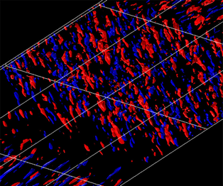
The increased drag in the 3DTBL region has a close relationship with the energized near-wall vortical structures by cross-flow. Figure 10 shows the isosurfaces of the instantaneous streamwise velocity fluctuation u and a positive value of the second invariant of the velocity gradient tensor $Q\textrm{(} \equiv{-} {u_{i,j}}{u_{j,i}}/2)$ with a magnified view in the near-wall region. After imposing ${W_S}$ at $x/{\theta _0} = 100$, the near-wall streaks and quasi-streamwise vortices are weakened due to a non-equilibrium effect. The latter becomes more pronounced as ${W_S}$ increases. On moving downstream, they then reappear and rotate their directions to those of the surface shear stress. Both the streaks and vortical structures become more energetic with increasing ${W_S}$ due to the increased straining by cross-flow, indicating that turbulence develops efficiently by cross-flow. In particular, near-wall vortices show a clustering for larger ${W_S}$. These behaviours can be quantified by examining the streamwise normal Reynolds stress $\overline {uu} /U_0^2$ and the enstrophy $\overline {\omega _i^\ast \omega _i^\ast }$ in the 3DTBL region (see figure 11) (note that a superscript * denotes the normalization by ${U_0}$ and ${\delta _{99}}$). Indeed, near-wall $\overline {\omega _i^\ast \omega _i^\ast }$ is more increased than $\overline {uu} /U_0^2$ as ${W_S}$ increases, consistent with the experimental results of Kiesow & Plesniak (Reference Kiesow and Plesniak2003). The increase is also observed for the energy dissipation rate ${\overline \varepsilon ^\ast }$ (distributions not shown here). This indicates that small scales are affected efficiently by cross-flow due to the increased mean straining. The behaviour of $\overline {\omega _i^\ast \omega _i^\ast }$ is also linked to the increased magnitude of the pressure fluctuation (distribution of ${p_{rms}}/\rho U_0^2$ not shown here), although their characteristic y scales are different (see Abe et al. Reference Abe, Antonia and Toh2018).

Figure 10.

Isosurfaces of u and Q for $R{e_{{\theta _0}}} = 300$ with ${W_S}/{U_0} = 0.5$, 1.0 and 1.5 : (a,c,e) red, $u/{U_0} \gt 0.15$; blue, $u/{U_0} \lt - 0.15$; (b) white, $Q\theta _0^2/U_0^2 \gt 0.01$; (d) white, $Q\theta _0^2/U_0^2 \gt 0.02$; (f) white, $Q\theta _0^2/U_0^2 \gt 0.04$. The fluid flows from bottom left to top right. The magnitudes of ${W_S}/{U_0}$ are 0.5 (a,b), 1.0 (c,d) and 1.5 (e,f), respectively. Note that the data below $y/{\delta _{99,0}} \approx 0.2$ have been plotted for highlighting the near-wall structures. The data shown have been obtained with ${L_{x,{W_S}}} = 200{\theta _0}$.

Figure 11.

Distributions of $\overline {uu} /U_0^2$ and $\overline {\omega _i^\ast \omega _i^\ast }$ in the 3DTBL region ($x/{\theta _0} = 275$) for $R{e_{{\theta _0}}} = 300$ with varying ${W_S}$: (a) $\overline {uu} /U_0^2$; and (b) $\overline {\omega _i^\ast \omega _i^\ast }$. The data shown have been obtained with ${L_{x,{W_S}}} = 200{\theta _0}$.

4.3. Reynolds stress and energy redistribution

We now discuss the near-wall distributions of the Reynolds stress and the energy redistribution. Figure 12(a–d) shows the distributions of the inner-normalized Reynolds normal stresses (i.e. $\overline {{u^ + }{u^ + }}$, $\overline {{v^ + }{v^ + }}$ and $\overline {{w^ + }{w^ + }}$) and Reynolds shear stress (i.e. $- \overline {{u^ + }{v^ + }}$) at a downstream station of the 3DTBL region ($x/{\theta _0} = 275$). Whilst all the Reynolds normal stresses normalized by $U_0^2$ increase with cross-flow, the inner-normalized Reynolds normal stresses exhibit a different behaviour. That is, $\overline {{u^ + }{u^ + }}$ decreases and $\overline {{w^ + }{w^ + }}$ increases (figure 12a,c) with increasing ${W_S}$; and $\overline {{v^ + }{v^ + }}$ (figure 12b) decreases slightly. Also, ${k^ + }$ (not shown here) increases gradually with increasing ${W_S}$ due to the increase in Reynolds number in a 3DTBL. This indicates that the anisotropy in the Reynolds normal stress is altered with increasing ${W_S}$. The primary Reynolds shear stress ($- \overline {{u^ + }{v^ + }}$) also decreases with increasing ${W_S}$, as observed in the recent DNS work by Lozano-Durán et al. (Reference Lozano-Durán, Giometto, Park and Moin2020) in a turbulent channel flow with a sudden spanwise pressure gradient. Not only the inactive motion ($\overline {{u^ + }{u^ + }}$ and $\overline {{w^ + }{w^ + }}$) but also the active motion ($\overline {{v^ + }{v^ + }}$ and $- \overline {{u^ + }{v^ + }}$) are changed in a 3DTBL. Note that, given the original idea of Townsend's (Reference Townsend1976) hypothesis, ‘inactive’ denotes a smaller contribution of larger motions to the Reynolds shear stress compared to that of smaller motions, while ‘active’ refers to the contribution exclusively to the Reynolds shear stress; see § 5.3 of Hwang (Reference Hwang2015). In this sense, large scales contain half of the Reynold shear stress in the log region or the outer region of a pipe flow (Guala, Hommema & Adrian Reference Guala, Hommema and Adrian2006) and of a channel and 2DTBL (Balakumar & Adrian Reference Balakumar and Adrian2007) (see also the spectral analysis in § 5.3).

Figure 12.

Distributions of the inner-normalized Reynolds stresses and the pressure strain terms in the 3DTBL region ($x/{\theta _0} = 275$) for $R{e_{{\theta _0}}} = 300$ with varying ${W_S}$: (a) $\overline {{u^ + }{u^ + }}$; (b) $\overline {{v^ + }{v^ + }}$; (c) $\overline {{w^ + }{w^ + }}$; (d) $-\overline{u^+v^+}$; (e) $\phi _{11}^ +$; (f) $\phi _{22}^ +$; (g) $\phi _{33}^ +$; and (h) $\phi _{12}^ +$. The data shown have been obtained with ${L_{x,{W_S}}} = 200{\theta _0}$.

To gain further insight into the variation of the Reynolds stresses, we here examine the pressure strain term (see figure 12e–h), which can be obtained by splitting the VPG ($\varPi _{ij}^ +$) into the pressure strain ($\phi _{ij}^ +$) and pressure diffusion ($\varphi _{ij}^ +$) terms, respectively:

(4.7)\begin{equation}\varPi _{ij}^ +{=} \underbrace{{\overline {{p^ + }\left( {\frac{{\partial u_i^ + }}{{\partial x_j^ + }} + \frac{{\partial u_j^ + }}{{\partial x_i^ + }}} \right)} }}_{{\phi _{ij}^ + }}\underbrace{{ - \left( {\frac{\partial }{{\partial x_i^ + }}\overline {u_j^ + {p^ + }} + \frac{\partial }{{\partial x_j^ + }}\overline {u_i^ + {p^ + }} } \right)}}_{{\varphi _{ij}^ + }}.\end{equation}

The pressure strain term is responsible for the energy redistribution for the Reynolds normal stress but for the destruction for the Reynolds shear stress. In a 2DTBL, the pressure strain plays a role in redistributing the energy from $\overline {uu}$ to $\overline {vv}$ and $\overline {ww}$. In the present 3DTBL, once the magnitude of $\overline {ww} /U_\tau ^2$ exceeds that of $\overline {uu} /U_\tau ^2$, the pressure strain for $\overline {uu}$ and $\overline {ww}$ show negative and positive values, respectively The energy redistribution for the inactive motion ($\overline {uu}$ and $\overline {ww}$) is indeed varied as the magnitude of cross-flow increases, whereas $\phi _{22}^ +$ for the active motion ($\overline {vv}$) decreases slightly. This indicates that the energy redistributes from $\overline {ww}$ to $\overline {uu}$ in the 3DTBL region when ${W_S}$ becomes sufficiently large. The largest values of $\phi _{11}^ +$ and $\phi _{33}^ +$ (≈ 0.08) are approximately one-fifth of the maximum value of $P_{11}^ +$ (≈ 0.5) in a 2DTBL. The magnitude of $\phi _{12}^ +$ (and thus the active motion) also decreases with increasing ${W_S}$, which was recently pointed out by Lozano-Durán et al. (Reference Lozano-Durán, Giometto, Park and Moin2020) in a turbulent channel flow with a sudden spanwise pressure gradient. They associated this behaviour with the self-similar behaviour in a 3DTBL. The self-similarity will be discussed in the next section. The present results indicate that the pressure strain term may not be dismissed when considering the modelling of $\overline {{u_i}{u_j}}$ in a 3DTBL.

5.1. Momentum thickness and skin friction coefficients

Figure 13 shows the distributions of the streamwise and spanwise momentum thicknesses, $\theta$ and ${\theta _z}$ (viz. (1.7) and (1.8)), and the momentum thickness Reynolds number, $R{e_\theta }$, as a function of $x/{\theta _0}$. For the streamwise momentum thickness $\theta$, the magnitude increases almost linearly with $x/{\theta _0}$. The imposition of ${W_S}$ yields an increase in $\theta$, where the rate of increase is greater for a larger ${W_S}$ (see figure 13b). The increased momentum thickness is essentially associated with inviscid skewing since the latter yields the deficit of $\overline U$. The increased magnitude of $\theta$ is also linked to that of ${C_{f,x}}$ (see figure 14a) as $\partial \theta /\partial x = {C_{f,x}}/2$ in the present flow due to the absence of the streamwise mean pressure gradient. The momentum thickness Reynolds number $R{e_\theta }$ thus depends intrinsically on both cross-flow and Reynolds number (see figure 13a). For the largest $R{e_{{\theta _0}}}$ and ${W_S}$ (i.e. $R{e_{{\theta _0}}} = 900$ and ${W_S}/{U_0} = 2$), $R{e_\theta }$ indeed varies from 900 (at the inlet) to 1550 (at the outlet). For the spanwise momentum thickness ${\theta _z}$, on the other hand, the magnitude for ${W_S}/{U_0} = 1$ increases with a ${x^{1/2}}$ dependence in the 3DTBL region for all three Reynolds numbers (see figure 13c), which corroborates the LES result of Kannepalli & Piomelli (Reference Kannepalli and Piomelli2000) for $R{e_\theta } \approx 1100$. The rate of increase for ${W_S}/{U_0} = 1$ is identical with that of Antonia & Luxton (Reference Antonia and Luxton1971) in their experiment in TBLs on the sudden change of the surface condition. However, ${\theta _z}$ develops more significantly for ${W_S}/{U_0} = 2$ than for ${W_S}/{U_0} = 1$, the former showing a departure from a ${x^{1/2}}$ dependence (see figure 13d). This latter trend seems to hold for a further larger ${W_S}$. The ${x^{1/2}}$ behaviour is essentially associated with the Stokes layer ${\theta _z} = \sqrt {\nu t}$, whereas the departure from the ${x^{1/2}}$ behaviour is due to the increased turbulent eddy viscosity ${\theta _z} = \sqrt {{\nu_{t,z}}t}$ (see figure 22(b) where the magnitude of ${\nu _{t,z}}/{\nu _{t,x}}$ increases with cross-flow at a large Re). The latter behaviour was also reported in the recent temporally developing DNS work of Lozano-Durán et al. (Reference Lozano-Durán, Giometto, Park and Moin2020).

Figure 13.

Distributions of $R{e_\theta }$, $\theta /{\theta _0}$ and ${\theta _z}/{\theta _0}$ as functions of $x/{\theta _0}$: (a) $R{e_\theta }$; (b) $\theta /{\theta _0}$ for $R{e_{{\theta _0}}} = 900$ with ${W_S}/{U_0} = 1$ and 2; (c) ${\theta _z}/{\theta _0}$ for $R{e_{{\theta _0}}} = 300$, 600 and 900 with ${W_S}/{U_0} = 1$; and (d) ${\theta _z}/{\theta _0}$ for $R{e_{{\theta _0}}} = 900$ with ${W_S}/{U_0} = 1$ and 2. The data shown have been obtained with ${L_{x,{W_S}}} = 100{\theta _0}$.

Figure 14.

Distributions of ${C_{f,x}}$ and ${C_{f,z}}$ as functions of $x/{\theta _0}$: (a) ${C_{f,x}}$ for $R{e_{{\theta _0}}} = 300$, 600 and 900 with ${W_S}/{U_0} = 1$; (b) ${C_{f,x}}$ for $R{e_{{\theta _0}}} = 900$ with ${W_S}/{U_0} = 1$ and 2; (c) ${C_{f,z}}$ for $R{e_{{\theta _0}}} = 300$, 600 and 900 with ${W_S}/{U_0} = 1$; and (d) ${C_{f,z}}$ for $R{e_{{\theta _0}}} = 900$ with ${W_S}/{U_0} = 1$ and 2. The data shown have been obtained with ${L_{x,{W_S}}} = 100{\theta _0}$.

Figure 14(a,c) shows the distributions of the streamwise and spanwise skin friction coefficients, ${C_{f,x}}$ and ${C_{f,z}}$, as a function of $x/{\theta _0}$ for all three Reynolds numbers with ${W_S}/{U_0} = 1$. Also compared are the LES data of Kannepalli & Piomelli (Reference Kannepalli and Piomelli2000) and the experimental data of Driver & Hebbar (Reference Driver and Hebbar1987) – their Reynolds numbers in a near-trailing edge of the 3DTBL region are $R{e_\theta } \approx 1100$ and 6000, respectively. After imposing ${W_S}$, we see a sudden decrease in the magnitudes of ${C_{f,x}}$ and ${C_{f,z}}$ for all three Reynolds numbers. The streamwise locations at which both ${C_{f,x}}$ and ${C_{f,z}}$ attain near-plateaus become smaller in terms of $x/{\theta _0}$ as the Reynolds number increases, while that for ${C_{f,x}}$ is not obtained for $R{e_{{\theta _0}}} = 300$ using ${L_{x,{W_S}}} = 100{\theta _0}$. The streamwise extent for obtaining a plateau in ${C_{f,x}}$ is $150{\theta _0}$, $165{\theta _0}$ and $40{\theta _0}$ (or, equivalently, 18δ ₀, 8δ ₀ and 5δ ₀) for $R{e_{{\theta _0}}} = 300$, 600 and 900, respectively (note that 150θ ₀ for $R{e_{{\theta _0}}} = 300$ has been obtained from the data using ${L_{x,{W_S}}} = 200{\theta _0}$ and 300θ ₀ shown in § 3.1). Note that ${C_{f,x}}$ obtained from the LES of Kannepalli & Piomelli (Reference Kannepalli and Piomelli2000) does not exhibit a plateau in the 3DTBL region, which seems to be due to the coarse streamwise spatial resolution in their simulation given that the agreement with the data for $R{e_{{\theta _0}}} = 600$ is excellent except for the 3DTBL region. The streamwise extent for $R{e_{{\theta _0}}} = 900$ (i.e. 5δ ₀ or $40{\theta _0}$) is approximately half that of Lohmann (Reference Lohmann1976) in this spinning cylinder experiment. The reason for the difference is likely to be because the imposition of ${W_S}$ yields a 3DTBL more efficiently over a flat plate than over a spinning cylinder. With increasing ${W_S}$, the streamwise locations at which both ${C_{f,x}}$ and ${C_{f,z}}$ attain near-plateaus remain essentially unchanged, whereas the magnitudes for ${W_S}/{U_0} = 2$ is greater than that for ${W_S}/{U_0} = 1$ (see figure 14b,d) as observed in Lohmann's (Reference Lohmann1976) experiment. The increased magnitudes of ${C_{f,x}}$ and ${C_{f,z}}$ are intrinsically associated with the energized vortical structures, as will be discussed in § 5.3.

In the recovery region, the magnitude of ${C_{f,x}}$ tends to approach that of a 2DTBL when $x/{\theta _0}$ reaches approximately 300. The Reynolds-number dependence of ${C_{f,x}}$ is also significant. In the latter context, Kannepalli & Piomelli (Reference Kannepalli and Piomelli2000) used a power-law relation on the basis of a 1/7 power-law mean velocity in a 2DTBL, i.e.

(5.1)\begin{equation}{C_{f,x}} = 0.020Re _\delta ^{ - 1/6}\textrm{,}\end{equation}

(see (6-68) of White Reference White1991), for estimating the Reynolds-number dependence (here ${Re _\delta }$ denotes the Reynolds number based on ${U_0}$ and ${\delta _{99}}$). They noted that, if the experimental ${C_{f,x}}$ by Driver & Johnston (Reference Driver and Johnston1990) is multiplied by ${\textrm{(}{Re _{\delta ,exp }}/{Re _{\delta ,LES}})^{1/6}}$, the resulting ${C_{f,x}}$ agrees well with the LES data of Kannepalli & Piomelli (Reference Kannepalli and Piomelli2000). Close inspection of the present DNS data at $x/{\theta _0} = 300$ has shown that, while the prediction of (5.1) is excellent for $R{e_{{\theta _0}}} = 300$, (5.1) underestimates ${C_{f,x}}$ by approximately 14 % for $R{e_{{\theta _0}}} = 900$. The latter result is attributed to the increased momentum thickness and Reynolds number in the 3DTBL and recovery regions owing to the effect of three-dimensionality (see figure 13c,d), whilst the boundary layer thickness remains invariably unchanged by cross-flow (the distribution is not shown here). Indeed, the power-law relation of Smits, Matheson & Joubert (Reference Smits, Matheson and Joubert1983), viz.

(5.2)\begin{equation}{C_{f,x}} = 0.024Re _\theta ^{ - 1/4}\textrm{,}\end{equation}

which predicts ${C_{f,x}}$ in a 2DTBL excellently over a wide range of Reynolds number (see Schlatter & Örlü Reference Schlatter and Örlü2010), leads to a better prediction of ${C_{f,x}}$ for $R{e_{{\theta _0}}} = 900$ in the recovery region (i.e. the difference between the DNS data and (5.2) is approximately 5 % for $R{e_{{\theta _0}}} = 900$ at $x/{\theta _0} = 300$).

To examine the Re dependence of ${C_{f,x}}$ and ${C_{f,z}}$ further, figure 15 shows the distributions of inner-normalized viscous (${C_{f,x\,vis}}$ and ${C_{f,z\,vis}}$) and turbulent (${C_{f,x\,turb}}$ and ${C_{f,z\,turb}}$) parts in the mean energy balances (i.e. (4.2) and (4.5)) as a function of $x/{\theta _0}$ for $R{e_{{\theta _0}}} = 300$, 600 and 900 with ${W_S}/{U_0} = 1$. In the 2DTBL region ($0 \le x/{\theta _0} \le 100$), $({2^{1/2}}/C_f^{3/2}){C_{f,x\,vis}}$ remains essentially unchanged independently of the Reynolds number (figure 15a), whilst $({2^{1/2}}/C_f^{3/2}){C_{f,x\,turb}}$ increases with increasing Reynolds number (figure 15b). This latter behaviour is consistent with the Re dependence in a 2-D flow by Renard & Deck (Reference Renard and Deck2016), Abe & Antonia (Reference Abe and Antonia2016) and Wei (Reference Wei2018). In the 3DTBL region ($100 \le x/{\theta _0} \le 200$), the magnitudes of both the viscous and turbulent parts decrease significantly due to the change of the surface shear-stress direction, and depend less on the Reynolds number at a downstream station of a 3DTBL. The latter Re independence is most likely due to the effect of the mean spanwise shear resulting from the imposition of ${W_S}$. For all three Reynolds numbers, the magnitude of ${C_{f,z\,turb}}$ is greater than that of ${C_{f,x\,turb}}$, which highlights that, in a 3DTBL, $\overline {uv}$ is less efficient in extracting energy from mean flow than $\overline {vw}$. Also, the increase in ${W_S}$ yields less extraction of energy from $\overline {uv}$, while ${C_{f,z\,turb}}$ (i.e. the energy extracted from $\overline {vw}$) contributes almost exclusively to ${C_{f\,turb}}$ (the distributions for ${W_S}/{U_0} = 2$ are not shown here). In the recovery region (${200 \le x/{\theta _0} \le 400}$), there is an increased magnitude of the turbulent part (${C_{f,x\,turb}}$) for a larger Reynolds number (figure 15b). Also, non-zero values of ${C_{f,z\,vis}}$ and ${C_{f,z\,turb}}$ are observed for the three Reynolds numbers. These behaviours underline that the effect of three-dimensionality propagates into the recovery region. This point will be discussed further in § 5.5.

Figure 15.

Distributions of terms on the right-hand side of (4.2) and (4.5) as functions of $x/{\theta _0}$ for $R{e_{{\theta _0}}} = 300$, 600 and 900 with ${W_S}/{U_0} = 1$: (a) $({{2^{1/2}}/C_f^{3/2}} ){C_{f,x\,vis}}$ and $({{2^{1/2}}/C_f^{3/2}} ){C_{f,z\,vis}}$; and (b) $({{2^{1/2}}/C_f^{3/2}} ){C_{f,x\,turb}}$ and $({{2^{1/2}}/C_f^{3/2}} ){C_{f,z\,turb}}$. The data shown have been obtained with ${L_{x,{W_S}}} = 100{\theta _0}$.

5.2. Departure from the ‘law of the wall’ in a non-equilibrium 3DTBL

Here, we discuss the ‘law of the wall’ in a non-equilibrium 3DTBL. In this context, the inner-layer scaling of the relative mean velocity (or, equivalently, the mean velocity magnitude), i.e.

(5.3)\begin{equation}{Q_r} \equiv {({\overline U ^2} + {(\overline W - {W_S})^2})^{1/2}},\end{equation}

has been intensively examined in a 3DTBL. There have been a number of observations indicating that the law of the wall, viz. (1.3), holds approximately in a shear-driven 3DTBL but with a larger magnitude of the von Kármán constant κ (see, for example, Bissonnette & Mellor Reference Bissonnette and Mellor1974; Pierce & McAllister Reference Pierce and McAllister1983; Moin et al. Reference Moin, Shih, Driver and Mansour1990) than $\kappa = 0.39$ in a 2DTBL (see Marusic et al. Reference Marusic, Monty, Hultmark and Smits2013). Given that the present 3DTBL will eventually approach the collateral state at a far-downstream station, the departure from the classical log law is intrinsically associated with a 3-D effect in a 3DTBL where there is a close relationship between a deficit of $\overline U$ and inviscid skewing (i.e. three-dimensionality) (see § 3.2).

Also, the classical inner scaling for the energy dissipation rate $\overline \varepsilon $ may be expressed as

(5.4)\begin{equation}{\overline \varepsilon ^ + } \equiv \overline \varepsilon \nu /U_\tau ^4 = 1/\kappa {y^ + }.\end{equation}

In the latter context, Abe & Antonia (Reference Abe and Antonia2016) made the matching argument to $\overline \varepsilon $ in a turbulent channel flow on the basis of the scaling arguments of Townsend (Reference Townsend1976) (see § 8.8 of his book). They obtained the following relation by assuming that the Reynolds number is large enough to have a clear distinction between inner and outer regions, and there is a region where the inner and outer scalings overlap, viz.

(5.5)\begin{equation}\overline \varepsilon y/U_\tau ^3 = 1/{\kappa _\varepsilon },\end{equation}

where ${\kappa _\varepsilon }$ is a constant. In (5.5), the relevant length scale is the distance from the wall, y, to be distinguished unambiguously. Note that ${\kappa _\varepsilon }$ is identical with $\kappa$ when the Reynolds number is sufficiently large enough to establish the velocity log law, where the constant shear stress (i.e. $\tau \simeq \rho U_\tau ^2$) and energy equilibrium (i.e. ${P_k} \simeq \overline \varepsilon $) assumptions also hold. Abe & Antonia (Reference Abe and Antonia2016) noted that $\overline \varepsilon y/U_\tau ^3$ approaches 2.54 (i.e. $1/{\kappa _\varepsilon } = 1/0.39$) in a channel, pipe and ZPG 2DTBL where the finite Re correction is required for a channel and a pipe due to the presence of the mean pressure gradient (see relations (4.22) and (4.23) of their paper).

Figure 16(a,b) shows the distributions of the inner-normalized mean velocity magnitude ${Q_r}$ and energy dissipation rate $\overline \varepsilon $, respectively, with the semi-logarithmic coordinates, for $R{e_{{\theta _0}}} = 300$, 600 and 900 with ${W_S}/{U_0} = 1.0$ and for $R{e_{{\theta _0}}} = 900$ with ${W_S}/{U_0} = 2.0$ in a near-equilibrium 3DTBL ($x/{\theta _0} = 175$). As the Reynolds number increases, the magnitude of $Q_r^ + \textrm{(} = {Q_r}/{U_\tau })$ becomes smaller away from the wall than in a 2DTBL. For $R{e_{{\theta _0}}} = 900$, the velocity log law (i.e. (1.3)) tends to hold but with a larger magnitude of the von Kármán constant $\kappa = 0.44$, in particular, for a larger ${W_S}$, i.e. ${W_S}/{U_0} = 2$ (see figure 16a), where the experimental data of Lohmann (Reference Lohmann1976) for ${W_S}/{U_0} = 1.75$ agree reasonably well with the present distribution for $Q_r^ +$ for ${W_S}/{U_0} = 2.0$; the constant shear stress (i.e. $\tau \simeq \rho U_\tau ^2$) and energy equilibrium (i.e. ${P_k} \simeq \overline \varepsilon $) assumptions also hold approximately for $R{e_{{\theta _0}}} = 900$ with ${W_S}/{U_0} = 2.0$ (the distributions are not shown here). In the latter region, the production of k (i.e. ${P_k} \equiv{-} \overline {{u_i}{u_j}} {S_{ij}}$) shows a smaller magnitude than for a 2DTBL (see figure 16c) (note that ${S_{ij}} \equiv ({\overline U _{i,j}} + {\overline U _{j,i}})/2$), which indicates that the present 3DTBL is less efficient in extracting energy from the mean velocity than in a 2DTBL.

Figure 16.

Distributions of $Q_r^ +$, ${\overline \varepsilon ^ + }$, ${P_k}y/U_\tau ^3$ and $\overline \varepsilon y/U_\tau ^3$ in the 3DTBL region ($x/{\theta _0} = 175$): (a) $Q_r^ +$ for $R{e_{{\theta _0}}} = 300$, 600 and 900 with ${W_S}/{U_0} = 1$ and for $R{e_{{\theta _0}}} = 900$ with ${W_S}/{U_0} = 2$; (b) ${\overline \varepsilon ^ + }$ or $R{e_{{\theta _0}}} = 300$, 600 and 900 with ${W_S}/{U_0} = 1$ and for $R{e_{{\theta _0}}} = 900$ with ${W_S}/{U_0} = 2$; (c) ${P_k}y/U_\tau ^3$ for $R{e_{{\theta _0}}} = 900$ with ${W_S}/{U_0} = 1$ and 2; and (d) $\overline \varepsilon y/U_\tau ^3$ for $R{e_{{\theta _0}}} = 900$ with ${W_S}/{U_0} = 1$ and 2. The data shown have been obtained with ${L_{x,{W_S}}} = 100{\theta _0}$. Also plotted for comparison are the DNS data of a ZPG 2DTBL for $R{e_\theta } = 1000$ obtained in the present work.

We also note that ${\overline \varepsilon ^ + }$ shows a better collapse for ${y^ + } \gt 20$ than $Q_r^ +$, where (5.5) with ${\kappa _\varepsilon } = 0.44$ provides a good fit to the DNS data (see figure 16b,d). Indeed, an apparent plateau appears in the distribution of $\overline \varepsilon y/U_\tau ^3$ in the region y⁺ = 20 to $y/{\delta _{99}} = 0.15$ (see figure 16d). This underlines that the overlap scaling holds more clearly for small scales than for large scales. The constant value of $\overline \varepsilon y/U_\tau ^3$ (i.e. (5.5)) is approximately 2.27, i.e. $1/{\kappa _\varepsilon } = 1/0.44$. Indeed, ${\kappa _\varepsilon }$ is identical with $\kappa$ when $R{e_{{\theta _0}}} = 900$. The implication at higher Reynolds number is that small scales are likely to lose the Re dependence more rapidly than large scales given a more distinct overlap scaling for $\overline \varepsilon $ than for $\overline U$; see also the DNS works in a turbulent channel flow by Abe & Antonia (Reference Abe and Antonia2016, Reference Abe and Antonia2017), who noted that the overlap scaling for the energy and scalar dissipation rates is in fact established at a smaller value of Re_τ than that at which the mean velocity and scalar log laws hold. Also, the clear plateau of $\overline \varepsilon y/U_\tau ^3$ (see the distribution in figure 16(d) for a larger ${W_S}$ case) indicates self-similarity in small scales, which is intrinsically due to the mean spanwise shear arising from ${W_S}$. This point will be discussed further in the next subsection by focusing on the most energetic spanwise wavelengths of velocity fluctuations.

5.3. Turbulence structures and energetic spanwise scales in a non-equilibrium 3DTBL

In this subsection, we first discuss asymmetric turbulence structures observed in the present 3DTBL. Figure 17 shows the contours in the y–z plane of the instantaneous streamwise velocity fluctuation u together with those of a positive value of Q for the three Reynolds numbers in a near-equilibrium 3DTBL ($x/{\theta _0} = 175$). As the Reynolds number increases, large-scale toppling u structures dominate in the outer region where the negative u structures preferentially correlate with the positive Q structures, the latter being stretched by cross-flow. Indeed, not only near-wall streaks but also outer-layer structures exhibit asymmetries due to the straining by cross-flow, which are reminiscent of the ‘toppling structures' hypothesized by Bradshaw & Pontikos (Reference Bradshaw and Pontikos1985). The energized vortical structures are intrinsically associated with the abruptly increased drag (figure 14). We note that, for the largest $R{e_{{\theta _0}}}$ with a large ${W_S}$ (i.e. $R{e_{{\theta _0}}} = 900$ and ${W_S}/{U_0} = 2$), both the u and Q structures are stretched significantly by cross-flow, showing asymmetries with approximately −30° (see figure 17d). The asymmetric vortical structures are most likely associated with the excellent overlap scaling established for the energy dissipation rate $\overline \varepsilon $ (figure 16d). This figure also highlights an intrinsic difference between the shear-driven and pressure-driven 3DTBLs, i.e. both the near-wall and outer-layer structures are affected by cross-flow in the shear-driven 3DTBL, whilst the outer-layer structures are exclusively altered in the pressure-driven 3DTBL (see figure 5 of Schlatter & Brandt Reference Schlatter, Brandt, Armenio, Geurts and Fröhlich2010).

Figure 17.

Contours in the y–z plane of u (colour) and a positive value of Q (line) in the 3DTBL region ($x/{\theta _0} = 175$) for $R{e_{{\theta _0}}} = 300$, 600 and 900: (a) $u/U_0\ \textrm{for}\ R{e_{{\theta _0}}} = 300$ with ${W_S}/{U_0} = 1$; (b) $u/U_0\ \textrm{for}\ R{e_{{\theta _0}}} = 600$ with ${W_S}/{U_0} = 1$; (c) $u/U_0\ \textrm{for}\ R{e_{{\theta _0}}} = 900$ with ${W_S}/{U_0} = 1$; and (d) $u/U_0\ \textrm{for}\ R{e_{{\theta _0}}} = 900$ with ${W_S}/{U_0} = 2$. The data shown have been obtained with ${L_{x,{W_S}}} = 100{\theta _0}$.

In figure 17, we also see an interface between the 2-D and 3-D structures at $y/{\delta _{99}} = 0.3\sim0.4$ for all three Reynolds numbers, which indicates that there is a reduced interaction between the inner and outer regions due to inviscid skewing. A similar behaviour was observed in the recent experimental work of Kevin et al. (Reference Kevin, Monty and Hutchins2019) in a 3DTBL with an angled ribbed surface. In this context, wall-normal two-point correlations, defined such that

(5.6)\begin{equation}{R_{aa}}({y_r},y) = \frac{{\overline {a({{y_r}} )a(y )} }}{{\,\overline {a({{y_r}} )a({{y_r}} )} }},\end{equation}

where y_r is a reference y location and $a \equiv u$, v or w, have been examined. Figure 18 shows the distributions of ${R_{uu}}({y_r},y)$ and ${R_{ww}}({y_r},y)$ in the 2DTBL and 3DTBL regions ($x/{\theta _0} = 50$ and 175) at two reference stations (i.e. ${y_r}/{\delta _{99}} \approx 0.1$ and 0.4). Note that, for this quantity, the data have been obtained for $R{e_{{\theta _0}}} = 300$ with ${W_S}/{U_0} = 1$, using ${L_{x,{W_S}}} = 100{\theta _0}$; averaging is based on a time period of t⁺ ≈ 2332. This figure indicates that the u and w correlations in the 3DTBL region approach zero at a smaller separation than those in the 2-D region (a similar trend is observed for the v correlations (not shown here)). This result highlights that there is a reduced correlation of velocity fluctuations in the present 3DTBL.

Figure 18.

Wall-normal two-point correlations for $R{e_{{\theta _0}}} = 300$ with ${W_S}/{U_0} = 1$: (a) ${R_{uu}} ({y_r},y)$; and (b) ${R_{ww}}({y_r},y)$. The averaging is based on a time period t⁺ ≈ 2332. The data have been obtained in both the 2DTBL and 3DTBL regions ($x/{\theta _0} = 50$ and 175) at two reference stations (i.e. ${y_r}/{\delta _{99}} \approx 0.1$ and 0.4). The data shown have been obtained with ${L_{x,{W_S}}} = 100{\theta _0}$.

It was also reported that in a 2DTBL (Hutchins & Marusic Reference Hutchins and Marusic2007) and a channel flow (Abe, Kawamura & Choi Reference Abe, Kawamura and Choi2004), large-scale footprints exist in the near-wall region as a consequence of the interaction between the inner and outer regions. Footprints are, however, not observed clearly in the present 3DTBL, which is most likely due to the reduced interaction between the inner and outer regions (the instantaneous u contours in the x–z plane near a wall are not shown here).

To provide further statistical evidence regarding the reduced interaction, one-dimensional spanwise spectra, i.e.

(5.7)\begin{equation}\int_0^\infty {{\phi _{aa}}({k_z})} \,\textrm{d}{k_z} = \int_0^\infty {{k_z}{\phi _{aa}}({k_z})} \,\textrm{d}(\log {k_z}) = \overline {aa} ,\end{equation}

have been investigated, where $\phi$ denotes the spectral density, k_z the spanwise wavenumber, λ_z  = 2π/k_z being the corresponding wavelengths, and $a \equiv u$, v or w. Figure 19(a,b) shows the ${\lambda _z}-y$ contours of the normalized premultiplied spanwise u spectra ${k_z}{\phi _{uu}}({k_z})$ (line) and uv co-spectra ${k_z}C{o_{uv}}({k_z})$ (colour) in the 2DTBL and 3DTBL regions ($x/{\theta _0} = 50$ and 175). Note that the uv co-spectra denote the real part of the cross-spectra; the same dataset as for the wall-normal two-point correlations has been used for this spectral analysis. In the 2-D region, the global spectral mode is observed in the outer region for both the u spectra and the uv co-spectra at large λ_z ($\ge 0.6{\delta _{99}}$) where the correspondence between the two spectra is reasonably good (see figure 19a). This behaviour highlights that the large-scale u structures are active for transporting the momentum.

Figure 19.

Contours in the ${\lambda _z}-y$ plane of normalized premultiplied spanwise u spectra ${k_z}{\phi _{uu}}({k_z})$, uv co-spectra ${k_z}C{o_{uv}}({k_z})$ and weighted uv co-spectra $- 4{k_z}(y/{\delta _{99}})C{o_{uv}}({k_z})(1 - y/{\delta _{99}})$ in the 2DTBL and 3DTBL regions ($x/{\theta _0} = 50$ and 175) for $R{e_{{\theta _0}}} = 300$ with ${W_S}/{U_0} = 1$: (a) ${k_z}{\phi _{uu}}({k_z})/U_0^2$ (line) and ${k_z}C{o_{uv}}({k_z})/U_0^2$ (colour) at $x/{\theta _0} = 50$; (b) ${k_z}{\phi _{uu}}({k_z})/U_0^2$ (line) and ${k_z}C{o_{uv}}({k_z})/U_0^2$ (colour) at $x/{\theta _0} = 175$; (c) $- 4{k_z}(y/{\delta _{99}})C{o_{uv}}({k_z})(1 - y/{\delta _{99}})/U_0^2$ at $x/{\theta _0} = 50$; and (d) $- 4{k_z}(y/{\delta _{99}})C{o_{uv}}({k_z})(1 - y/{\delta _{99}})/U_0^2$ at $x/{\theta _0} = 175$. The averaging is based on a time period t⁺ ≈ 2332. The data shown have been obtained with ${L_{x,{W_S}}} = 100{\theta _0}$.

The global mode, however, becomes weakened in the 3-D region, indicating the reduced interaction between the inner and outer regions (see figure 19b) – note that the reduced spectral energy in the outer layer is also observed for the premultiplied spanwise v and w spectra, ${k_z}{\phi _{vv}}({k_z})$ and ${k_z}{\phi _{ww}}({k_z})$ (not shown here) in the 3DTBL region. In particular, we observe the decreased magnitude of ${k_z}C{o_{uv}}({k_z})/U_0^2$ at $y/{\delta _{99}} = 0.3 \sim 0.4$ in the 3DTBL region, consistent with the reduced magnitude of $- \overline {uv}$ in the outer region. This reduced ${k_z}{\phi _{uu}}({k_z})/U_0^2$ is intrinsically associated with a smaller magnitude of ${C_{f,x\,turb}}$ than in the collateral state and thus the lower efficiency in extracting energy from the mean flow (see § 4.1).

In the latter context, it would also be instructive to pay attention to the spectral analysis by Deck et al. (Reference Deck, Renard, Laraufie and Weiss2014), who discussed how ${C_{f,x\,}}$ in a 2DTBL is related to the spatial changes in turbulence motions. They focused on the contribution of the $\overline {uv}$ term to ${C_{f,x\,}}$ in the FIK identity (Fukagata et al. Reference Fukagata, Iwamoto and Kasagi2002), and examined the streamwise weighted uv co-spectra, i.e. $- 4{k_x}(y/{\delta _{99}})C{o_{uv}}({k_x})(1 - y/{\delta _{99}})$. Note that k_x denotes the streamwise wavenumber; the factor of $(y/{\delta _{99}})$ arises from the $\overline {uv}$ term in the FIK identity. Deck et al. (Reference Deck, Renard, Laraufie and Weiss2014) noted that in a 2DTBL, large scales in the outer region make a major contribution to ${C_{f,x\,}}$. A similar inspection has been made for the present spanwise weighted spectra, i.e. $- 4{k_z}(y/{\delta _{99}})C{o_{uv}}({k_z})(1 - y/{\delta _{99}})$ (see figure 19c,d), which display an outer energetic mode more clearly than ${k_z}C{o_{uv}}({k_z})$ (see figure 19a,b) in both the 2DTBL and 3DTBL regions. Also, we see in figure 19(c,d) that the weighted co-spectra in a 3DTBL exhibit a decreased magnitude of the global energetic mode at large λ_z ($\ge 0.6{\delta _{99}}$) compared with those in a 2DTBL. This result underlines the close relationship between the reduced ${C_{f,x\,}}$ and the decreased interaction between the inner and outer regions in the 3DTBL region.

We next quantify the spanwise organization of the u structures in a 3DTBL with the use of the energy spectra. Figure 20(a) shows the spanwise spectral density of u, $k_z \phi_{uu}(k_z)$, normalized by $\overline{uu}$, at y/δ ₉₉ ≈ 0.2, compared with those in a 2DTBL (present DNS; Tomkins & Adrian Reference Tomkins and Adrian2005), channel flow (Hoyas & Jiménez Reference Hoyas and Jiménez2008; Abe et al. Reference Abe, Antonia and Toh2018) and pipe flow (Ahn et al. Reference Ahn, Lee, Lee, Kang and Sung2015). Abe et al. (Reference Abe, Antonia and Toh2018) noted that, while the outer flow is completely different between the internal and external flows (e.g. the presence of the λ_z/h = 1.3–1.6 or λ_z/R = 1.3 mode in the internal flows, where R denotes the pipe radius), there is some similarity in the spectral peak at a lower wavelength (λ_z/h = 0.8–0.9 (channel), λ_z/R = 0.7 (pipe) and λ_z/δ ₉₉ = 0.8 (boundary layer)). They associated this similarity with the fact that the magnitude of the von Kármán constant κ does not differ significantly between the three flows and is approximately 0.39 at extremely large Reynolds number (Marusic et al. Reference Marusic, Monty, Hultmark and Smits2013). Figure 20(a) highlights that the peak wavelength of ${k_z}{\phi _{uu}}({k_z})$ in a 3DTBL appears at a shorter wavelength than that in a 2DTBL, due to the turning of large-scale u structures by inviscid skewing (see figure 21, where the contours in the x–z plane of the instantaneous streamwise and spanwise velocity fluctuations, u and w, are shown for $R{e_{{\theta _0}}} = 900$ with ${W_S}/{U_0} = 1$ and 2 together with those in a 2DTBL).

Figure 20.

One-dimensional premultiplied spanwise u spectra at $y/{\delta _{99}} = 0.2$ of a 3DTBL and the most energetic spanwise scales, ${\lambda _{z,max}}$, obtained from peaks of premultiplied spanwise spectra below $y/{\delta _{99}} = 0.2$: (a) ${k_z}{\phi_{uu}}\left( {{k_z}} \right)/\overline {uu}$ for $R{e_{{\theta _0}}} = 900$ with ${W_S}/{U_0} = 1$ and 2; (b) ${\lambda_{z,max}}/{\delta_{99}}$ for u for $R{e_{{\theta _0}}} = 300$, 600 and 900 with ${W_S}/{U_0} = 1$ and 2; and (c) ${\lambda_{z,max}}/{\delta_{99}}$ for w for $R{e_{{\theta _0}}} = 300$, 600 and 900 with ${W_S}/{U_0} = 1$. In (a), the spectra are compared with those in a turbulent channel flow of Abe et al. (Reference Abe, Antonia and Toh2018) (black solid line) and Hoyas & Jiménez (Reference Hoyas and Jiménez2008) (black dashed line) for h⁺ = 1020 and 2003 at y/h = 0.2, respectively. Also included are the spectra of Tomkins & Adrian (Reference Tomkins and Adrian2005) in a ZPG TBL for δ⁺ = 2216 at y/δ = 0.2 (circle) and those of Ahn et al. (Reference Ahn, Lee, Lee, Kang and Sung2015) in a turbulent pipe for R⁺ = 3008 at y/R = 0.1 (triangle). In (b,c), the dashed lines denote the linear fittings. In (a–c), the data shown have been obtained with ${L_{x,{W_S}}} = 100{\theta _0}$.

Figure 21.

Contours in the x–z plane of u (colour) (a,c,e) and w (colour) (b,d,f) together with those of a positive value of Q (line) in 2DTBLs and 3DTBLs: (a) $u/U_0$ in a 2DTBL for $R{e_\theta } \approx 1000$; (b) $w/U_0$ in a 2DTBL for $R{e_\theta } \approx 1000$; (c) $u/U_0$ in a 3DTBL for $R{e_{{\theta _0}}} = 900$ with ${W_S}/{U_0} = 1$; (d) $w/U_0$ in a 3DTBL for $R{e_{{\theta _0}}} = 900$ with ${W_S}/{U_0} = 1$; (e) $u/U_0$ in a 3DTBL for $R{e_{{\theta _0}}} = 900$ with ${W_S}/{U_0} = 2$; and (f) $w/U_0$ in a 3DTBL for $R{e_{{\theta _0}}} = 900$ with ${W_S}/{U_0} = 2$. In (c–f), structures in the 3DTBL region have been visualized with an enlarged view; the data shown in these panels have been obtained with ${L_{x,{W_S}}} = 100{\theta _0}$. In (c,d) and (e,f), the solid lines denotes the direction of $\alpha ={-} 45^\circ$ and $- 60^\circ$, respectively, which correspond to the surface shear-stress direction in the collateral state.

We now examine the most energetic spanwise scales of the asymmetric u structures, ${\lambda _{z,max}}$, by plotting the peak wavelengths of the premultiplied spectra ${k_z}{\phi _{uu}}({k_z})$ below y/δ ₉₉ ≈ 0.2 in figure 20(b). Also plotted in figure 20(c) is the distribution of ${\lambda _{z,max}}$ for w for comparison. Note that the peak wavelength of the premultiplied spectrum corresponds to the most energetic scale contributing to the mean-square value; a least-squares fitting has been made for the spectral peak to obtain ${\lambda _{z,max}}$. While the self-similar behaviour is not observed clearly in a 2DTBL due to the effect of large scales (see Jiménez & Hoyas Reference Jiménez and Hoyas2008; Abe et al. Reference Abe, Antonia and Toh2018), the linear increase in ${\lambda _{z,max}}$ is indeed observed for the u spectra in a 3DTBL below y/δ ₉₉ = 0.2 for both ${W_S}/{U_0} = 1$ and 2. Note that in a 3DTBL, there is also a linear increase in ${\lambda _{z,max}}$ for the w spectra with ${W_S}/{U_0} = 1$ (figure 20c), but not with ${W_S}/{U_0} = 2$ (not shown here) due to the presence of large-scale elongated w structures (see figure 21f).

Given the notion of Nickels et al. (Reference Nickels, Marusic, Hafez, Hutchins and Chong2007) that any eddy with a size that scales with its distance from the wall may be considered to be attached to the wall, the well-established linear dependence of ${\lambda _{z,max}}$ for u in a 3DTBL is intrinsically associated with the attached-eddy hypothesis of Townsend (Reference Townsend1976). Inspection of the instantaneous u contours in the x–z plane (figure 21a,c,e) indicates that large-scale u structures become less anisotropic with increasing ${W_S}$. These results underline that the spanwise mean shear resulting from the imposition of ${W_S}$ yields a self-similar behaviour in the asymmetric u structures. The departure from self-similarity due to the large-scale contamination was indeed reported in a turbulent channel flow by Jiménez & Hoyas (Reference Jiménez and Hoyas2008), Hwang (Reference Hwang2015) and Abe, Antonia & Toh (Reference Abe, Antonia and Toh2018). Note that, while some u structure are aligned with the shear-stress direction in the collateral state (i.e. $\alpha ={-} 45^\circ$ and $- 60^\circ$) (see the black solid lines in figure 21c–f), most of the u structures are altered slowly compared with the w structures. This slow turning of the u structures is most likely associated with the slower approach to the collateral state for $\overline U$ than $\overline W$. We also note that ${\lambda _{z,max}}$ for w also shows a linear increase with respect to y for ${W_S}/{U_0} = 1$, but not for ${W_S}/{U_0} = 2$ (see figure 20c) since large scales dominate for w for a larger ${W_S}$ (see figure 21f).

As for vortical structures in a 2DTBL, Adrian, Meinhart & Tomkins (Reference Adrian, Meinhart and Tomkins2000) reported hairpin vortical structures and noted the relationship with the negative u structures. In the present 3DTBL, Kiesow & Plesniak (Reference Kiesow and Plesniak2003) hypothesized skewing of hairpin vortices. Inspection of the contours in the x–y plane (not shown) and x–z plane (figure 21) has revealed that, as observed in a 2DTBL by Adrian et al. (Reference Adrian, Meinhart and Tomkins2000), the low-momentum regions preferentially correlate with vortical structures. With increasing ${W_S}$, the correlation between the u structures and vortical structures becomes weaker due to the breakdown of large-scale u structures (figure 21c,e). On the other hand, the w structures tend to exhibit elongated structures in the shear-stress direction (see also the black solid line in figure 21f) where vortical structures are aligned with the w structures (figure 21d,f). Indeed, the vortical structures change their directions due to inviscid skewing.

5.4. Behaviour of the primary Reynolds shear stress $\overline {uv}$ in a non-equilibrium 3DTBL

Recently, Lozano-Durán et al. (Reference Lozano-Durán, Giometto, Park and Moin2020) discussed the reduced behaviour of the primary Reynolds shear stress $\overline {uv}$ in their 3-D channel DNS with a sudden imposition of mean spanwise pressure gradient. They explained it as a non-equilibrium effect rather than three-dimensionality. Here, we examine the behaviour of $\overline {uv}$ in the present 3DTBL and the implication for turbulence modelling.

Figure 22(a) shows the distributions of $\overline {uv}$, respectively, at a downstream station of the 3DTBL region ($x/{\theta _0} = 175$) for $R{e_{{\theta _0}}} = 900$ with ${W_S}/{U_0} = 1$ and 2. The magnitude of $- \overline {uv} /U_0^2$ in the inner region ($y/{\delta _{99}} \le 0.2$) is increased significantly with cross-flow, whereas there is a reduced magnitude of $- \overline {uv} /U_0^2$ in the outer region. The latter decrease is also observed in the recent experiment by Kevin et al. (Reference Kevin, Monty and Hutchins2019) in their 3DTBL on a ribbed surface. Close inspection of the instantaneous product uv (not shown here) shows a decrease in magnitude at the interface between the 2-D and 3-D structures (see figure 17 where the u contours in the y–z plane are shown), which supports the hypothesis of Bradshaw & Pontikos (Reference Bradshaw and Pontikos1985) that rapid decreases of shear stress are caused by the sideways tilting of the large eddies away from their preferred orientation. In the $uv$ co-spectra (see figure 19), we also see the statistical evidence on a decreased global mode at large λ_z ($\ge 0.6{\delta _{99}}$) in the 3DTBL region. These results indicate that the reduction in $\overline {uv} /U_0^2$ in the present shear-driven flow is intrinsically associated with a reduced interaction between the inner and outer regions due to inviscid skewing. Inspection of figure 22(a) has revealed that the relative reduction of $\overline {uv} /U_0^2$ (i.e. the dip at $y/{\delta _{99}} \approx 0.4$) to the value of a 2DTBL is approximately 25 %, the latter value being identical with the result of Lozano-Durán et al. (Reference Lozano-Durán, Giometto, Park and Moin2020) in the 3-D channel DNS. In the latter DNS, a mean spanwise pressure gradient is imposed, which is equivalent to applying a spanwise motion to the walls, in the opposite directions (this was pointed out by Dr G. N. Coleman, private communication 2019). There is thus a similarity between the present 3DTBL and that of Lozano-Durán et al. (Reference Lozano-Durán, Giometto, Park and Moin2020). In both 3DTBLs, the mean streamwise vorticity ${\overline \varOmega _x}$ propagates from the near-wall region to the outer layer. Also, a self-similar behaviour is observed. Given these similarities, a non-equilibrium effect reported by Lozano-Durán et al. (Reference Lozano-Durán, Giometto, Park and Moin2020) may involve a reduced interaction between the inner and outer regions due to three-dimensionality.

Figure 22.

Distributions of the outer-normalized $- \overline {uv}$, the correlation coefficient $- {R_{uv}}$, the turbulent eddy viscosity ratio ${\nu_{t,z}}/{\nu_{t,x}}$ and the structure parameter ${a_1}$ in the 3DTBL region ($x/{\theta _0} = 175$): (a) $- \overline {uv} /U_0^2$ for $R{e_{{\theta _0}}} = 900$ with ${W_S}/{U_0} = 1$ and 2; (b) ${\nu_{t,z}}/{\nu_{t,x}}$ for$R{e_{{\theta _0}}} = 900$ with ${W_S}/{U_0} = 1$ and 2; (c) $- {R_{uv}}$ for $R{e_{{\theta _0}}} = 300$, 600 and 900 with ${W_S}/{U_0} = 1$ and $R{e_{{\theta _0}}} = 900$ with ${W_S}/{U_0} = 2$; and (d) ${a_1}$ for $R{e_{{\theta _0}}} = 300$, 600 and 900 with ${W_S}/{U_0} = 1$ and $R{e_{{\theta _0}}} = 900$ with ${W_S}/{U_0} = 2$. The data shown have been obtained with ${L_{x,{W_S}}} = 100{\theta _0}$. Also plotted for comparison are the DNS data of a ZPG 2DTBL for $R{e_\theta } = 1000$ obtained in the present work.

At this x station ($x/{\theta _0} = 175$), there appear a deficit of $\overline U$ (not shown here) and also a decreased magnitude of the correlation coefficient $- {R_{uv}}({ ={-} \overline {uv} /{u_{rms}}{v_{rms}}} )$ as in the APG TBL (see figure 22c where the present $- {R_{uv}}$ is nearly identical with that of Gungor et al. (Reference Gungor, Maciel, Simens and Soria2014) in a strong APG 2DTBL; see also figure 11 from Abe (Reference Abe2019)). This result, however, does not imply the similarity between the present 3DTBL and APG 2DTBL. Figure 22(d) shows the distributions of the structure parameter ${a_1}$ in the 3DTBL region ($x/{\theta _0} = 175$). This figure highlights that the present magnitude attains ${a_1} \approx 0.14$ at $y/{\delta _{99}} \approx 0.1$ where there is a maximum streamwise mean velocity deficit (the distribution of $\overline U$ is not shown here). The present value of ${a_1}({\approx} 0.14)$ is greater than ${a_1} = 0.11$ in the APG TBL by Spalart & Watmuff (Reference Spalart and Watmuff1993). This result supports the finding of Coleman et al. (Reference Coleman, Kim and Spalart2000) that the impact of the APG on the outer-layer structure is more pronounced than that of the mean three-dimensionality. Also, the present distribution of ${a_1}$ in the inner region of a 3DTBL ($y/{\delta _{99}} \le 0.2$) agrees well with the experimental results of Littell & Eaton (Reference Littell and Eaton1994) in the rotating disk and the DNS and LES results of Spalart (Reference Spalart1989) and Wu & Squires (Reference Wu and Squires1997) in the equilibrium 3DTBL (see figure 22d).

On the other hand, as for $\overline {uv} /U_0^2$, the significant decrease in magnitude of ${a_1}$ is observed in the present 3DTBL, as in a ‘pressure-driven’ skewed TBL by Anderson & Eaton (Reference Anderson and Eaton1989). This supports the notion of Eaton (Reference Eaton1995) that the reduction of the Reynolds shear stress by the mean flow three-dimensionality is a common feature in 3DTBLs. Note that the reduction is also observed in the Reynolds normal stresses in the outer region – see figure 23(c,d) where the present DNS data for $\overline {uu} /U_0^2$ and $\overline {vv} /U_0^2$ agree well with the experiment by Kiesow & Plesniak (Reference Kiesow and Plesniak2003). As noted by Kiesow & Plesniak (Reference Kiesow and Plesniak2003), the near-wall Reynolds normal stresses, normalized by $U_0^2$, increase with the magnitude of cross-flow (the distribution of $\overline {ww} /U_0^2$ is not shown here). In particular, the two wall-parallel inactive motions (i.e. $\overline {uu} /U_0^2$ and $\overline {ww} /U_0^2$) increase significantly with ${W_S}$. For all three Reynolds numbers (i.e. $R{e_{{\theta _0}}} = 300$, 600 and 900), the energy redistribution between the Reynolds normal stresses is also altered when ${W_S}/{U_0} = 2$, i.e. the energy redistributes from $\overline {ww}$ to $\overline {uu}$ away from the wall independently of the Reynolds number (the distributions of the pressure strain for $R{e_{{\theta _0}}} = 600$ and 900 are not shown here).

Figure 23.

Distributions of the normalized mixing and dissipation lengths (${\ell _m}$ and ${\ell _d}$) and Reynolds normal stresses in the 3DTBL region ($x/{\theta _0} = 175$) for $R{e_{{\theta _0}}} = 300$, 600 and 900 with ${W_S}/{U_0} = 1$ and for $R{e_{{\theta _0}}} = 900$ with ${W_S}/{U_0} = 2$: (a) ${\ell _m}/{\delta _{99}}$; (b) ${\ell _d}/{\delta _{99}}$; (c) $\overline {uu} /U_0^2$; and (d) $\overline {vv} /U_0^2$. In (c,d), the triangle denotes the experimental data of Kiesow & Plesniak (Reference Kiesow and Plesniak2003) for $R{e_\theta } = 1450$. The data shown have been obtained with ${L_{x,{W_S}}} = 100{\theta _0}$. Also plotted for comparison are the DNS data of a ZPG 2DTBL for $R{e_\theta } = 1000$ obtained in the present work.

We now discuss the implication of the reduced $\overline {uv}$ for the turbulence modelling. The reduced magnitude of $\overline {uv}$ (figure 22a) implies a lag between the Reynolds stress vector and the mean strain-rate one, which is intrinsically linked to the anisotropy of the turbulent eddy viscosity (see Anderson & Eaton Reference Anderson and Eaton1989; Ӧlcmen & Simpson Reference Ӧlcmen and Simpson1995; Johnston & Flack Reference Johnston and Flack1996). The ratio of the spanwise eddy viscosity,

(5.8)\begin{equation}{\nu _{t,z}} = -\overline{vw} /(\partial \overline W /\partial y),\end{equation}

to the streamwise eddy viscosity,

(5.9)\begin{equation}{\nu _{t,x}} ={-} \overline {uv} /(\partial \overline U /\partial y),\end{equation}

has been intensively examined in 3DTBLs, where the magnitude is often below unity (see Anderson & Eaton Reference Anderson and Eaton1989; Ӧlcmen & Simpson Reference Ӧlcmen and Simpson1995; Johnston & Flack Reference Johnston and Flack1996). Figure 22(b) demonstrates that the present magnitude of ${\nu _{t,z}}/{\nu _{t,x}}$ is indeed below unity in the outer region of a near-equilibrium 3DTBL and decreases down to 0.6 at $y/{\delta _{99}} = 0.4 \sim 0.5$ since $\overline {vw} \gt \overline {uv}$ there.

On the other hand, the magnitude of ${\nu _{t,z}}/{\nu _{t,x}}$ is greater than unity in the inner region of a 3DTBL. These behaviours highlight the anisotropy of the turbulent eddy viscosity in the present non-equilibrium 3DTBL. In this context, Rotta (Reference Rotta, Durst, Launder, Schmidt and Whitelaw1979) introduced an empirical parameter T (being identical with the ratio ${\nu _{t,z}}/{\nu _{t,x}}$) into a mixing length model for predicting a non-equilibrium 3DTBL. While his model is not Galilean-invariant, it indeed provides an improved prediction (see Anderson & Eaton Reference Anderson and Eaton1989; Ӧlcmen & Simpson Reference Ӧlcmen and Simpson1993). In Rotta's (Reference Rotta, Durst, Launder, Schmidt and Whitelaw1979) model, the primary Reynolds shear stress is calculated such that

(5.10)\begin{equation}- \overline {uv} = {\nu _{t,xx}}(\partial \overline U /\partial y) + {\nu _{t,xz}}(\partial \overline W /\partial y),\end{equation}

where two anisotropic forms of the turbulent eddy viscosity, i.e.

(5.11)\begin{equation}{\nu _{t,xx}} = {\nu _t}({\overline U ^2} + T{\overline W ^2})/Q_r^2\end{equation}

and

(5.12)\begin{equation}{\nu _{t,xz}} = {\nu _t}(1 - T)\overline{U}\ \overline{W}/Q_r^2,\end{equation}

are used. Here, we test Rotta's T model for the present 3DTBL by inserting the current DNS datasets into the right-hand sides of (5.10)–(5.12). Note that in (5.11) and (5.12), the effective turbulent eddy viscosity ${\nu _t} ={-} \overline {{u_i}{u_j}} {S_{ij}}/2{S_{kl}}{S_{kl}}$ (Spalart & Strelets Reference Spalart and Strelets2000) is used, which is a coordinate-invariant form and can be described as a least-squares fit to the Reynolds stress tensor. The optimal value of T differs in different flows (see Anderson & Eaton Reference Anderson and Eaton1989; Ӧlcmen & Simpson Reference Ӧlcmen and Simpson1993). In the present study, T = 0.9 is used for yielding the closest prediction to the DNS data. Indeed, the calculated $\overline {uv}$ agrees reasonably well with the DNS data in the present flow (see figure 22a), which indicates that the effect of three-dimensionality (i.e. the Reynolds stress lags behind the mean strain) cannot be dismissed when predicting the present flow.

Also, the mixing length ${\ell _m}$ for a 3DTBL may be obtained as

(5.13)\begin{equation}{\ell _m} = {{{({{\overline {vw} }^2} + {{\overline {uv} }^2})}^{1/4}}} \left/\left[{{{\left( {\frac{{\partial \overline U }}{{\partial y}}} \right)}^2} + {{\left( {\frac{{\partial \overline W }}{{\partial y}}} \right)}^2}}\right]^{1/2}\right.\end{equation}

(see Rotta Reference Rotta, Durst, Launder, Schmidt and Whitelaw1979; Bradshaw Reference Bradshaw1987), which is a coordinate-invariant form. Figure 23(a) shows the distributions of normalized ${\ell _m}$ in the 3DTBL region ($x/{\theta _0} = 175$).Clearly, the distributions follow the relation ${\ell _m} \approx 0.4y$ in the inner region ($y/{\delta _{99}} \le 0.1$), whereas the magnitudes are reduced significantly in the outer region (i.e. $0.1 \le y/{\delta _{99}} \le 0.6$) and the latter are below the value of a 2DTBL (i.e. ${\ell _m}/{\delta _{99}} \approx 0.1$). This result also agrees reasonably well with the PIV measurement by Kiesow & Plesniak (Reference Kiesow and Plesniak2003) in the present flow (see figure 23a). A similar decrease is observed in the dissipation length scale, viz.

(5.14)\begin{equation}{\ell _d} = {({\overline {vw} ^2} + {\overline {uv} ^2})^{3/2}}/\overline \varepsilon \end{equation}

(see figure 23b). This result is not surprising given that a near-energy-equilibrium condition (i.e. ${P_k} \simeq \overline \varepsilon $) is satisfied approximately there (the distribution is not shown here). These results indicate that the effect of three-dimensionality dominates in the 3DTBL region, which has an important implication for turbulence modelling, viz. the length scale reduction needs to be taken into account when developing a turbulence model for a 3DTBL given that the turbulent eddy viscosity is represented by ${\nu _t} \propto {k^{1/2}}\ell$.

5.5. Recovery to a 2DTBL

Finally, we discuss the recovery of a 3DTBL to a normal 2DTBL in light of the seminal work of Antonia & Luxton (Reference Antonia and Luxton1971) on a sudden change of a surface condition given the presence of the internal boundary layer (i.e. after turning off ${W_S}$, a new boundary layer develops inside a 3DTBL).

Figure 24 shows the distributions of the inner-normalized ${Q_r}$ for $R{e_{{\theta _0}}} = 300$, 600 and 900 with ${W_S}/{U_0} = 1$ and for $R{e_{{\theta _0}}} = 900$ with ${W_S}/{U_0} = 2$ at a downstream station of the recovery region ($x/{\theta _0} = 300$) in which the spanwise friction coefficient becomes negligibly small (figure 14c,d). While the near-wall distributions become closer to those in a 2DTBL, we see a discernible departure from the classical log law in ${Q_r}$ away from the wall. The reason for the departure is due to the effect of a 3DTBL persisting in this region, in particular, for a larger ${W_S}$ (i.e. the cross-flow (the distribution of $\overline W$ is not shown here) is still present away from the wall). On the other hand, there is rather quick recovery to a 2DTBL in the inner region. In this context, Bassina, Strelets & Spalart (Reference Bassina, Strelets and Spalart2001) examined the performance of several eddy viscosity models, i.e. SA (Spalart & Allmaras Reference Spalart and Allmaras1994) and SST (Menter Reference Menter1994) models, in the recovery region of the present flow. They noted that, while the eddy viscosity models cannot reproduce the significant deviation between the Reynolds stress and mean shear-stress vectors present in the recovery region, the agreement of the computations with the data on the mean flow characteristics is unexpectedly good. They pointed out that the inner layer has much control over the skin friction and does not contain protracted 3-D effects. This latter behaviour is consistent with that observed in the present DNS.

Figure 24.

Distributions of the normalized $Q_r^{}$, ${\ell _m}$, k, ${p_{rms}}$ in the recovery region ($x/{\theta _0} = 300$): (a) $Q_r^ +$ for $R{e_{{\theta _0}}} = 300$, 600 and 900 with ${W_S}/{U_0} = 1$ and $R{e_{{\theta _0}}} = 900$ with ${W_S}/{U_0} = 2$; (b) ${\ell _m}/{\delta _{99}}$ for $R{e_{{\theta _0}}} = 300$, 600 and 900 with ${W_S}/{U_0} = 1$ and for $R{e_{{\theta _0}}} = 900$ with ${W_S}/{U_0} = 2$; (c) ${k^ + }$ for $R{e_{{\theta _0}}} = 900$ with ${W_S}/{U_0} = 1$ and 2; and (d) $p_{rms}^ +$ for $R{e_{{\theta _0}}} = 900$ with ${W_S}/{U_0} = 1$ and 2. The data shown have been obtained with ${L_{x,{W_S}}} = 100{\theta _0}$. Also plotted for comparison are the DNS data of a ZPG 2DTBL for $R{e_\theta } = 1000$ obtained in the present work.

As for turbulence statistics, a large outer peak appears for ${k^ + }$ (figure 24c) and $p_{rms}^ +$ (figure 24d) especially for a larger ${W_S}$, where the distribution of $p_{rms}^ +$ shows a larger magnitude than that for a 2DTBL. Inspection of the instantaneous fields shows that vortical structures are energized in the outer layer compared with those in a 2DTBL (see figure 25). Also, whilst the negative region of the large-scale u structures is preferentially associated with vortical structures in the outer region of a 2DTBL (see figures 21a and 25a; also Adrian et al. Reference Adrian, Meinhart and Tomkins2000), both the positive and negative regions of the u structures tend to correlate with vortical structures in the outer layer of the recovery region (see figure 25b), which are also active in generating the Reynolds shear stress (the instantaneous product uv is not shown here). This latter behaviour is intrinsically linked to the increased outer peaks of ${k^ + }$ (figure 24c) and ${\tau ^ + }$ (not shown here) in the recovery region, which indicates that the recovery to the ZPG TBL state is slow due to the effect of three-dimensionality. Also, wall-attached structures with a size of ${\delta _{99}}$ are observed for the pressure fluctuation p (see figure 25c), which are not only inclined in the z direction but also become energetic due to the effect of three-dimensionality. This behaviour is consistent with the significant increase in $p_{rms}^ +$ in the recovery region (see figure 24d).

Figure 25.

Contours in the y–z plane of u and p (colour) and a positive value of Q (line) in the recovery region compared with those in a ZPG 2DTBL: (a) $u/U_0$ for a ZPG 2DTBL for $R{e_\theta } = 1000$; (b) $u/U_0$ at $x/{\theta _0} = 300$ for $R{e_{{\theta _0}}} = 900$ with ${W_S}/{U_0} = 2$; and (c) $p/\rho U_0^2$ at $x/{\theta _0} = 300$ for $R{e_{{\theta _0}}} = 900$ with ${W_S}/{U_0} = 2$. The data shown have been obtained with ${L_{x,{W_S}}} = 100{\theta _0}$.

We also note that, in the outer region of the recovery region, the magnitude of the mixing length ${\ell _m}/{\delta _{99}}$ is smaller than the value of a 2DTBL (i.e. ${\ell _m}/{\delta _{99}} \approx 0.1$) (see figure 24b). The magnitude of ${a_1}$ is also smaller than those for a 2DTBL (not shown here) since the Reynolds normal stress is more enhanced by the effect of three-dimensionality than the Reynolds shear stress (see the large outer peak in the distribution of ${k^ + }$ shown in figure 24c). A similar trend is observed in the experiment of Antonia & Luxton (Reference Antonia and Luxton1972) on the sudden change of the surface condition (i.e. a rough to smooth wall surface), while the data of Antonia & Luxton (Reference Antonia and Luxton1972) show a much larger decrease than the present DNS data. The difference between the present study and that of Antonia & Luxton (Reference Antonia and Luxton1972) is most likely because the effect of a rough wall diffuses more significantly into the outer region than that of inviscid skewing. These results underline that the effect of three-dimensionality persists in the recovery region.