1 Introduction
Flow over an inclined plate easily separates from the sharp leading edge and generates a leading-edge vortex. For translating two-dimensional (2-D) plates, the leading-edge vortex grows and starts shedding (Sarpkaya Reference Sarpkaya1975; Beem, Rival & Triantafyllou Reference Beem, Rival and Triantafyllou2012; Mancini et al.
Reference Mancini, Manar, Granlund, Ol and Jones2015), but for three-dimensional (3-D) rotating plates it remains stable (Ellington et al.
Reference Ellington, den berg, Wilmott and Thomas1996; Tangler Reference Tangler2004; Shyy & Liu Reference Shyy and Liu2007; Muijres et al.
Reference Muijres, Johansson, Barfield, Wolf, Spedding. and Hedenström2008; Lentink et al.
Reference Lentink, Dickson, van Leeuwen and Dickinson2009). The stable leading-edge vortex has also been reported in aquatic swimming (Borazjani & Daghooghi Reference Borazjani and Daghooghi2013; Bottom et al.
Reference Bottom, Borazjani, Blevins and Lauder2016; Liu et al.
Reference Liu, Ren, Dong, Akanyeti, Liao and Lauder2017). For translating plates, at a low angle of attack and moderate Reynolds numbers (
 $10^{6}>Re>10^{4}$
), the separated flow transitions to turbulent and flow reattaches due to the mixing of the high-momentum flow in the shear layer with the low-momentum flow near the wall (Alam & Sandham Reference Alam and Sandham2000). Flow separation decreases lift and increases drag, leading to the aerodynamic stall of aerial vehicles. To overcome this drawback, passive flow control methods such as vortex generators (Lin Reference Lin2002), boundary layer trip (Braslow, Hicks & Harris Reference Braslow, Hicks and Harris1966), etc., and active flow control methods such as periodic excitation (Greenblatt & Wygnanski Reference Greenblatt and Wygnanski2000) or steady blowing (Lachmann Reference Lachmann2014) are employed. With the development of smart materials, surface actuators are becoming practicable as active flow control tools. DeMauro et al. (Reference DeMauro, DellOrso, Zaremski, Leong and Amitay2015) and Jones et al. (Reference Jones, Santer, Debiasi and Papadakis2018) improved aerodynamic performance by producing a standing-wave oscillation on the suction side of an airfoil. Recently, travelling waves have been created experimentally on flexible structures using multiple piezoelectric actuators (Bani-Hani & Karami Reference Bani-Hani and Karami2015). The amplitudes of such travelling waves are low, which has motivated us to numerically investigate the effects of low-amplitude travelling waves on flow separation and aerodynamic performance of a thin inclined plate.
The inspiration to use travelling waves for reducing flow separation comes from aquatic animals. Large-amplitude travelling waves are used by aquatic animals for propulsion, which is also thought to reattach the flow on their bodies (Anderson, McGillis & Grosenbaugh Reference Anderson, McGillis and Grosenbaugh2001). Borazjani & Sotiropoulos (Reference Borazjani and Sotiropoulos2008) showed that the travelling waves over a fish body reattach the flow and decrease the form drag but increase the viscous drag. Also, Wu, Wang & Wu (Reference Wu, Wang and Wu2007) controlled the flow separation of a circular cylinder by employing a travelling wave over the cylinder. Lighthill (Reference Lighthill1960) and Wu (Reference Wu1961) analytically investigated the propulsion characteristics of a plate undergoing an undulatory motion to understand the basic principle of fish swimming hydrodynamics. Lighthill (Reference Lighthill1960) proposed elongated body theory (EBT), in which the instantaneous lift of an undulating slender body (low thickness) is scaled with the added-mass force (reactive force). The reactive force produced by the undulation generates a thrust that increases as wave speed (
 $C$
) is increased. It also predicts zero net lateral force (force perpendicular to the body) as the flow is assumed potential, which remains periodic. Furthermore, the investigations of Taneda (Reference Taneda1976) and Shen et al. (Reference Shen, Zhang, Yue and Triantafyllou2003) also show that travelling waves reattach the flow on wavy surfaces. Taneda (Reference Taneda1976) experimentally observed that, when the wave speed is less than the flow speed (
 $C<U$
), the flow separates from the first crest of the horizontal plate, but it becomes attached when it is more than the flow speed (i.e.
 $C>U$
). These visualizations were confirmed by the simulations of Shen et al. (Reference Shen, Zhang, Yue and Triantafyllou2003) for a turbulent channel flow. They also reported that turbulence intensity reduces by the increase in
 $C/U$
. Although they reported
 $C$
to be the main parameter for flow reattachment of an undulating flat plate, the effect of wavelength (
 $\unicode[STIX]{x1D706}$
) was not considered separately. In fact, our results (§ 3) show that the separation can decrease when
 $C$
is reduced, in contrast to the theory, by decreasing wavelength. Note that the nature of separation for flow over an inclined plate is completely different from that for wavy bodies with zero angle of attack (Taneda Reference Taneda1976; Shen et al.
Reference Shen, Zhang, Yue and Triantafyllou2003; Borazjani & Sotiropoulos Reference Borazjani and Sotiropoulos2008; Quinn, Lauder & Smits Reference Quinn, Lauder and Smits2014) as will be discussed in § 4.
To investigate if low-amplitude travelling waves, which can be generated experimentally using piezoelectric actuators (Bani-Hani & Karami Reference Bani-Hani and Karami2015), can reduce flow separation, the flow separation and aerodynamic performance of 3-D undulating thin inclined plates are numerically investigated. The effect of different wavelengths (
 $\unicode[STIX]{x1D706}$
) and frequencies
 $(f)$
is discussed and compared with the scaling of vorticity and thrust derived by EBT. The time-averaged, phase-averaged and instantaneous results are presented in § 3. The results are discussed in § 4, and § 5 summarizes the findings of this work. The validations and the derivation of scalings are presented in appendices.
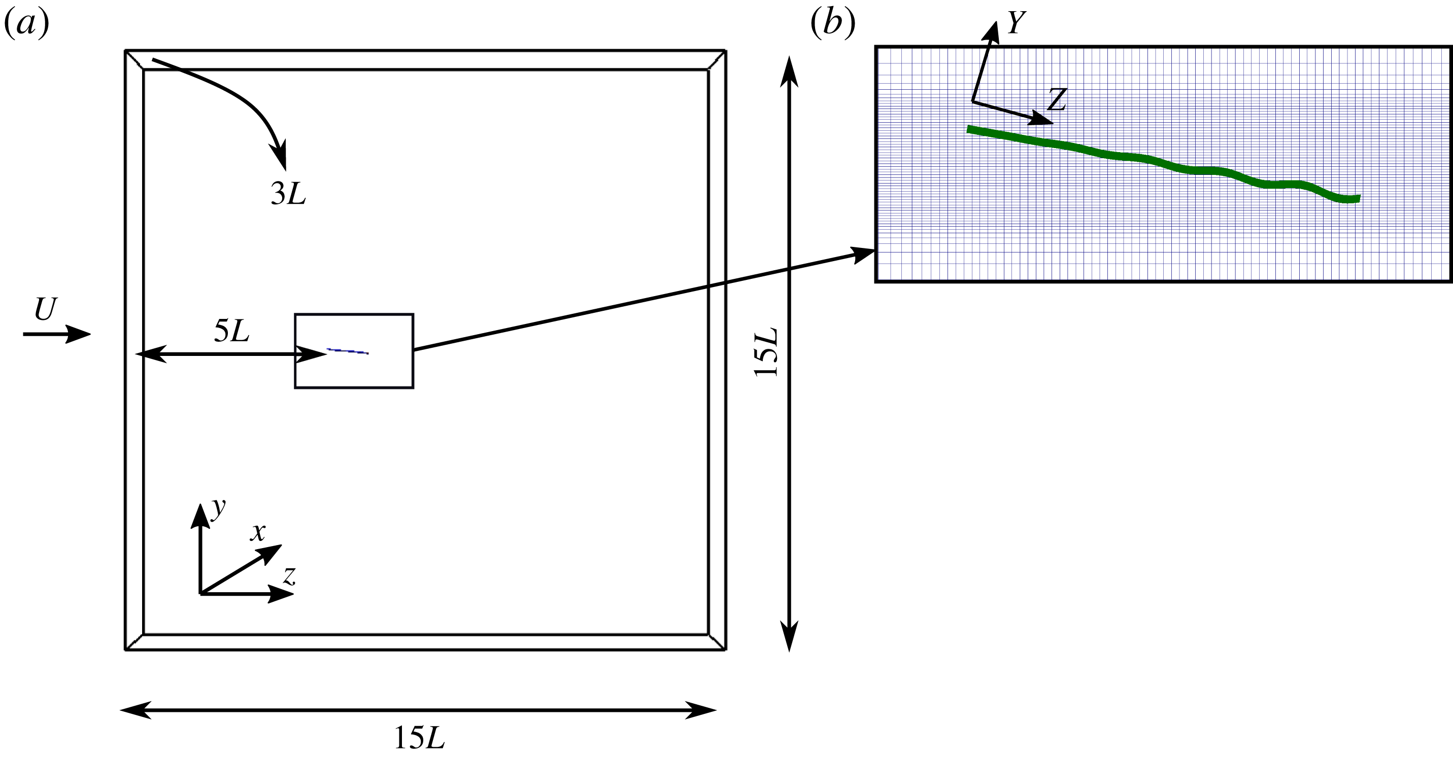
(a) The computational domain and immersed body. (b) The 2-D section of the undulating plate in the computational grid. The motion is defined in the rotated frame and then transformed into the flow frame. Every fifth and every other grid line is shown in the
 $y$
and
 $z$
directions, respectively.

2 Materials and methods
Numerical simulations are performed for an inclined 3-D plate of aspect ratio 2 at the angle of attack of
 $10^{\circ }$
. The angle of attack is chosen to be
 $10^{\circ }$
because it is high enough to generate an unstable leading-edge vortex (LEV) for a wing with an aspect ratio of 1.5–3 (Pelletier & Mueller Reference Pelletier and Mueller2000; Visbal Reference Visbal2011). The plate chord length is
 $L$
, its thickness is
 $0.02L$
and the spanwise length is
 $2L$
. The free-stream velocity (
 $U$
) and the chord length (
 $L$
) are the reference velocity and length scales for non-dimensionalization, respectively. As shown in figure 1(a), flow is in the frame
 $(x,y,z)$
where
 $x$
,
 $y$
and
 $z$
are the spanwise, vertical and streamwise coordinates, respectively. Simulations are performed for both flat and undulatory inclined plates. The prescribed undulatory motion is a backward travelling wave that starts from
 $0.1L$
of the leading edge with a linearly increasing amplitude towards the trailing edge. To calculate the new position of the inclined plate under motion in the flow frame, a local frame
 $(X,Y,Z)$
is defined, which is rotated by the angle of attack (figure 1
b). The undulations
 $h$
are prescribed perpendicular to the plate, i.e. along the
 $Y$
direction in the rotated frame, based on the travelling wave equation
 $$\begin{eqnarray}h(Z,t)=a(Z)\sin (\unicode[STIX]{x1D6FA}^{\ast }t^{\ast }-2\unicode[STIX]{x03C0}Z^{\ast }/\unicode[STIX]{x1D706}^{\ast }),\end{eqnarray}$$
where
 $h$
is the lateral undulation,
 $Z^{\ast }=Z/L$
is the non-dimensional chordwise length in local coordinates and
 $a(Z)$
is the amplitude of the wave. The origin is at the top surface of the leading edge such that
 $Z=0$
and
 $Z=L$
are the leading edge and trailing edge, respectively. Frequency (
 $f$
) and wavelength (
 $\unicode[STIX]{x1D706}$
) are the varying terms of the wave, where
 $\unicode[STIX]{x1D706}^{\ast }=\unicode[STIX]{x1D706}/L$
is non-dimensionalized with
 $L$
. The amplitude envelope of the travelling wave is
 $a(Z)=0$
for
 $Z<0.1L$
and
 $a(Z)=a_{max}(Z-0.1L)/0.9L$
for
 $Z>0.1L$
, where
 $a_{max}=0.01L$
is the dimensional maximum amplitude of the wave. The reduced frequency is
 $f^{\ast }=fL/U$
,
 $\unicode[STIX]{x1D6FA}^{\ast }=2\unicode[STIX]{x03C0}f^{\ast }$
,
 $\unicode[STIX]{x1D703}=10^{\circ }$
is the angle of attack and
 $t^{\ast }=tU/L$
is the non-dimensional time, where
 $t$
is the dimensional time. The maximum amplitude
 $a_{max}$
is chosen to be small because travelling waves generated by smart structures have small amplitudes (Bani-Hani & Karami Reference Bani-Hani and Karami2015). Herein, symbol
 $^{\ast }$
denotes non-dimensional parameters, including length, time, velocity and vorticity. However, the notation for non-dimensional pressure and
 $Q$
-criterion are
 $p$
and
 $Q$
, respectively.
The Reynolds number in this study is
 $Re=LU/\unicode[STIX]{x1D708}=20\,000$
(where
 $\unicode[STIX]{x1D708}$
is kinematic viscosity). Varying parameters in these simulations are
 $f^{\ast }$
and
 $\unicode[STIX]{x1D706}^{\ast }$
, which have the ranges of (0–30) and (0.15–2.0), respectively. The Strouhal number, defined as
 $St=2a_{max}\,f/U$
, is in the range of (0.0–0.6), which is close to the range (0.2–0.7) typically observed in nature (Triantafyllou, Triantafyllou & Yue Reference Triantafyllou, Triantafyllou and Yue2000). More specifically, the simulations for undulating cases are carried out for three reduced frequencies,
 $f^{\ast }=(6,20,30)$
and six wavelengths
 $\unicode[STIX]{x1D706}^{\ast }=(0.15,0.2,0.5,1.0,2.0,1000.0)$
. The different
 $f^{\ast }$
and
 $\unicode[STIX]{x1D706}^{\ast }$
for each case are presented later in table 2. Case 1 is a flat inclined plate and case 9 (
 $\unicode[STIX]{x1D706}=1000.0$
) is a pitching plate. It should be noted that, when the wavelength is increased, the wave speed (
 $C/U=f^{\ast }\unicode[STIX]{x1D706}^{\ast }$
) increases and the wave steepness (
 $a_{max}^{\ast }/\unicode[STIX]{x1D706}^{\ast }$
) decreases.
To discuss the impact of undulations on the flow over the plate, scalings for velocity, vorticity and thrust are derived based on EBT (Lighthill Reference Lighthill1960) in appendix C. EBT is based on inviscid slender-body theory, i.e. the flow perturbation in the lateral direction is much smaller than in the axial direction. In addition, the pressure of the adjacent fluid on to the swimmer scales with the reactive force that is related to the fluid acceleration. Although EBT is based on the inviscid flow assumption and low velocity undulation, it will be demonstrated in § 3 that such scalings can predict the patterns of the simulations for flow characteristics such as lateral velocity, out-of-plane vorticity and relative drag force compared to the flat inclined plate (thrust force) because the main mechanism for thrust generation in EBT, i.e. the added mass, is dominant in high-frequency undulations.
2.1 Numerical method and computational details
The equations governing the flow are the unsteady 3-D incompressible Navier–Stokes and continuity equations. The governing equations are discretized via a central scheme and integrated in time using a second-order fractional methodology on hybrid staggered/non-staggered grids (Ge & Sotiropoulos Reference Ge and Sotiropoulos2007; Borazjani, Ge & Sotiropoulos Reference Borazjani, Ge and Sotiropoulos2008). The momentum equations are solved with a Newton–Krylov solver and the pressure Poisson equation is solved using a GMRES solver with a multigrid preconditioner (Ge & Sotiropoulos Reference Ge and Sotiropoulos2007; Borazjani et al. Reference Borazjani, Ge and Sotiropoulos2008). The moving boundaries are handled using the sharp-interface immersed boundary (IB) method described in detail in previous publications (Ge & Sotiropoulos Reference Ge and Sotiropoulos2007; Borazjani et al. Reference Borazjani, Ge and Sotiropoulos2008). In this method, the background grid is fixed and does not move with the boundaries, i.e. the plate with the prescribed motion (2.1) is discretized by the triangular mesh and placed as a sharp-interface IB over the fixed background grid. The grid nodes inside the immersed boundary (solid nodes) are blanked out, while the velocity on the nodes that are exterior, but adjacent, to the immersed boundary (IB nodes) are reconstructed using an interpolation along the normal to the boundary (Gilmanov & Sotiropoulos Reference Gilmanov and Sotiropoulos2005). The background grid nodes are classified into solid, fluid and IB nodes by an efficient ray-tracing algorithm (Borazjani et al. Reference Borazjani, Ge and Sotiropoulos2008). The method is fully validated for flows with moving boundaries (Borazjani et al. Reference Borazjani, Ge and Sotiropoulos2008, Reference Borazjani, Sotiropoulos, Tytell and Lauder2012; Asgharzadeh & Borazjani Reference Asgharzadeh and Borazjani2017) and also has been used in different applications (Daghooghi & Borazjani Reference Daghooghi and Borazjani2015; Hedayat, Asgharzadeh & Borazjani Reference Hedayat, Asgharzadeh and Borazjani2017; Asadi, Asgharzadeh & Borazjani Reference Asadi, Asgharzadeh and Borazjani2018; Akbarzadeh & Borazjani Reference Akbarzadeh and Borazjani2019; Asgharzadeh et al. Reference Asgharzadeh, Asadi, Meng and Borazjani2019; Hedayat & Borazjani Reference Hedayat and Borazjani2019).
For large-eddy simulation (LES) modelling, a dynamic Smagorinsky model (Lilly Reference Lilly1992) is employed to compute the subgrid stress tensor. The details of our LES modelling are described in previous publications (Kang et al.
Reference Kang, Borazjani, Colby and Sotiropoulos2012; Bottom et al.
Reference Bottom, Borazjani, Blevins and Lauder2016). To show the validity of our LES for separated flows and computing the hydrodynamic forces, a LES validation study is performed by simulating the flow over a 2-D flat inclined plate at various angles of attack in appendix A. To further validate the LES for moving boundaries, simulations of a pitching NACA0012 airfoil at
 $Re=12\,600$
are performed. The results and detail of this simulation are given in appendix B.
The computational domain of the simulation (figure 1
a) is a cuboid with dimensions
 $3L\times 15L\times 15L$
, which is discretized with
 $81\times 421\times 301$
grid nodes in
 $x$
,
 $y$
and
 $z$
directions, respectively. The thin plate is placed
 $5L$
from the inlet boundary and centred in the lateral (
 $y$
) and spanwise (
 $x$
) directions as shown in figure 1(a). To resolve the flow near the thin plate, a curvilinear grid is built with a constant resolution of
 $0.0013L$
and
 $0.01L$
in a rectangle of
 $0.34L\times L$
in the
 $y$
and
 $z$
directions, respectively, which contains the undulating plate and stretches out to the domain boundaries using a hyperbolic function as shown in figure 1(b). The grid resolution is constant in the
 $x$
direction and grid spacing normal to the wall is 1.5 wall units (
 $y^{+}=u_{\unicode[STIX]{x1D70F}}\unicode[STIX]{x1D6FF}/\unicode[STIX]{x1D708}=1.5$
, where
 $u_{\unicode[STIX]{x1D70F}}$
is the friction velocity and
 $\unicode[STIX]{x1D6FF}$
is the normal distance of the IB node to the plate). The first grid point is within the viscous sublayer (
 $y^{+}<5$
) of the turbulent boundary layer, which is enough for reconstructing the velocity of the IB nodes with a linear interpolation (Pope & Pope Reference Pope and Pope2000). The non-dimensional time step for the flat inclined plate is 0.0025 and for the rest of the cases is
 $1/(240f^{\ast })$
. The sensitivity of the simulations to the grid and time-step size is investigated in the next subsection.
The boundary condition on the lateral and spanwise boundaries is the slip wall, the inlet is uniform (plug) flow, and the outlet is a Neumann boundary with a correction to satisfy the conservation of mass. All simulations in which the plate is undulating are initialized by the flow field of the flat inclined plate where both leading- and trailing-edge vortices are shedding. Furthermore, the hydrodynamic forces (lift and thrust) are computed by integrating the pressure and viscous forces acting on the plate.
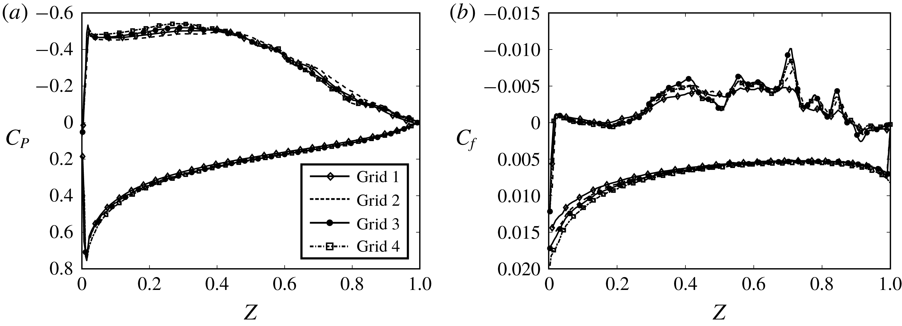
The (a) pressure and (b) skin-friction coefficient along the chord on the midplane of the flat inclined plate for four different grids. The upper and lower curves are the coefficients on the suction and pressure sides of the plate, respectively.

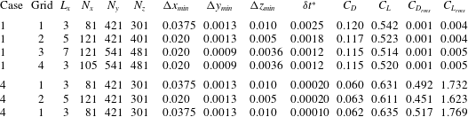
The details of grid and time-step size for the grid sensitivity studies. A grid sensitivity study for a flat inclined plate (case 1) with four grids is performed. A grid sensitivity study with two grids as well as a time-step sensitivity study are performed for a high-frequency undulating plate (case 4,
 $f^{\ast }=20,~\unicode[STIX]{x1D706}^{\ast }=0.2$
). Here
 $\unicode[STIX]{x1D6FF}t^{\ast }$
is the non-dimensional time-step size,
 $L_{x}$
is the domain spanwise length,
 $C_{D_{rms}}$
and
 $C_{L_{rms}}$
are the root mean square (r.m.s.) values of lift fluctuations for drag and lift coefficients, respectively, and all hydrodynamic forces are non-dimensionalized with
 $\unicode[STIX]{x1D70C}U^{2}L^{2}$
, as the spanwise length of the plate is
 $2L$
(plate area is
 $L^{2}$
).

2.2 Grid and time-step sensitivity studies
A grid sensitivity study is performed to investigate the effect of mesh size and domain spanwise size on the pressure distribution and skin friction for the flat inclined plate with four grids (figure 2
a,b). In addition, a grid sensitivity study and a time-step sensitivity study are performed to ensure that the results of the simulations are time-step- and grid-independent for undulating cases. The details of grids, time step, mean lift and drag coefficients with their corresponding root-mean-square (r.m.s.) values of fluctuations are presented in table 1. Grid 2 has a higher resolution along the streamwise and spanwise directions, while grids 3 and 4 have a higher resolution in three directions, i.e. the grid spacing has decreased to 0.53, 0.69 and 0.33 of that of grid 1 in
 $x$
,
 $y$
and
 $z$
directions, respectively. The spanwise length of the domain has increased from 3 for grid 1 to 5 and 7 for grids 2 and 3, respectively, whereas grid 4 has the same domain size as grid 1. In fact, grid 4 has the same grid resolution near the thin plate as grid 3, while the same domain size as grid 1. Consequently, comparing the results of grids 1 and 4 (same domain size) reveals the effect of grid resolution, while comparing the results of grids 3 and 4 (same resolution) reveals the effect of the spanwise length of the numerical domain.
The grid sensitivity study for the flat inclined plate shows that the drag coefficient as well as the r.m.s. value of fluctuations vary less than 4 % for all four grids (table 1), and the lift coefficient decreases slightly (less than 6 %) as the grid becomes finer. Nevertheless, even the lift coefficient of the coarsest grid (
 $C_{L}=0.54$
for grid 1) is within the range of 0.48–0.54 reported for Reynolds numbers of
 $6\times 10^{4}$
to
 $20\times 10^{4}$
(Anderson Reference Anderson1985; Pelletier & Mueller Reference Pelletier and Mueller2000). Figure 2(a) shows the time-averaged pressure coefficient (
 $C_{p}=2p/\unicode[STIX]{x1D70C}U^{2}$
) on both sides of the plate for grids 1, 2, 3 and 4. As can be observed, the pressure coefficient is similar between the four grids. Figure 2(b) shows the skin-friction coefficient
 $C_{f}=(2/Re)(\unicode[STIX]{x2202}u_{z}^{\ast }/\unicode[STIX]{x2202}y^{\ast })$
along the plate on both sides of the plate, where
 $u_{z}^{\ast }$
is the non-dimensional streamwise velocity. As can be observed in figure 2(b), the curves of
 $C_{f}$
for all of the grids on the pressure side of the plate are approximately identical, but there are some discrepancies on the suction side where the flow is separated. The
 $C_{f}$
of grids 3 and 4 shows slightly higher fluctuations of the skin friction on the suction side, as they have a higher resolution. These discrepancies, nevertheless, do not influence the force coefficients (see table 1) because the friction force is significantly (an order of magnitude) smaller than the pressure force (
 $C_{f}\ll C_{p}$
, as observed in figure 2) and also the magnitude of
 $C_{f}$
on the suction side is small compared to that on the pressure side (see the profile of
 $C_{f}$
on both sides of the plate in figure 2
b). Based on these results, i.e. similarity of the pressure coefficients on the midplane for these grids (figure 2
a), observing very close lift coefficients (less than 6 % difference) and the similarity between skin-friction coefficients (figure 2
b), the spatial and spanwise lengths are enough to capture the flow physics and forces.
Another grid sensitivity study is also carried out for an undulating case with grids 1 and 2 by comparing the lift and drag coefficients and their corresponding r.m.s. fluctuations. The difference between the aerodynamic performances of the two grids is less than 6 %, and the difference between their r.m.s. values is less than 10 %. Based on the averaged forces and their r.m.s. values, we conclude that the undulating simulations are grid-insensitive as well. The time-step sensitivity study is performed with a time-step size
 $\unicode[STIX]{x1D6FF}t^{\ast }=1/(480f^{\ast })$
that is half of the original time-step size
 $\unicode[STIX]{x1D6FF}t^{\ast }=1/(240f^{\ast })$
used in this study. The averaged forces obtained from the time-step sensitivity study are similar and the difference between the r.m.s. values of the forces is around 5 % (table 1), which shows that the time step is small enough to capture the correct physics.
3 Results
To see the effect of undulation on flow separation, time-averaged results, including mean flow field and turbulence intensity, are presented in §§ 3.1 and 3.2. The mean and instantaneous aerodynamic forces are shown in § 3.3 and compared with the scalings obtained using EBT. Afterwards, the trends observed for mean flow separation and aerodynamic forces for different frequencies and wavelengths are discussed based on the phase-averaged flow in § 3.4 to identify the mechanisms affecting flow reattachment by the travelling waves.
3.1 The effect of travelling waves on the flow separation of the mean flow
In this section, the mean flow is visualized to see the impact of both frequency and wavelength of travelling waves on flow separation. The impact of frequency and wavelength of the travelling wave on flow separation is reported quantitatively by defining a reattachment length for the separated flow. The reattachment length is defined here as the distance between the leading edge and the point where the time-averaged streamwise velocity becomes greater than zero (
 $u_{z}>0$
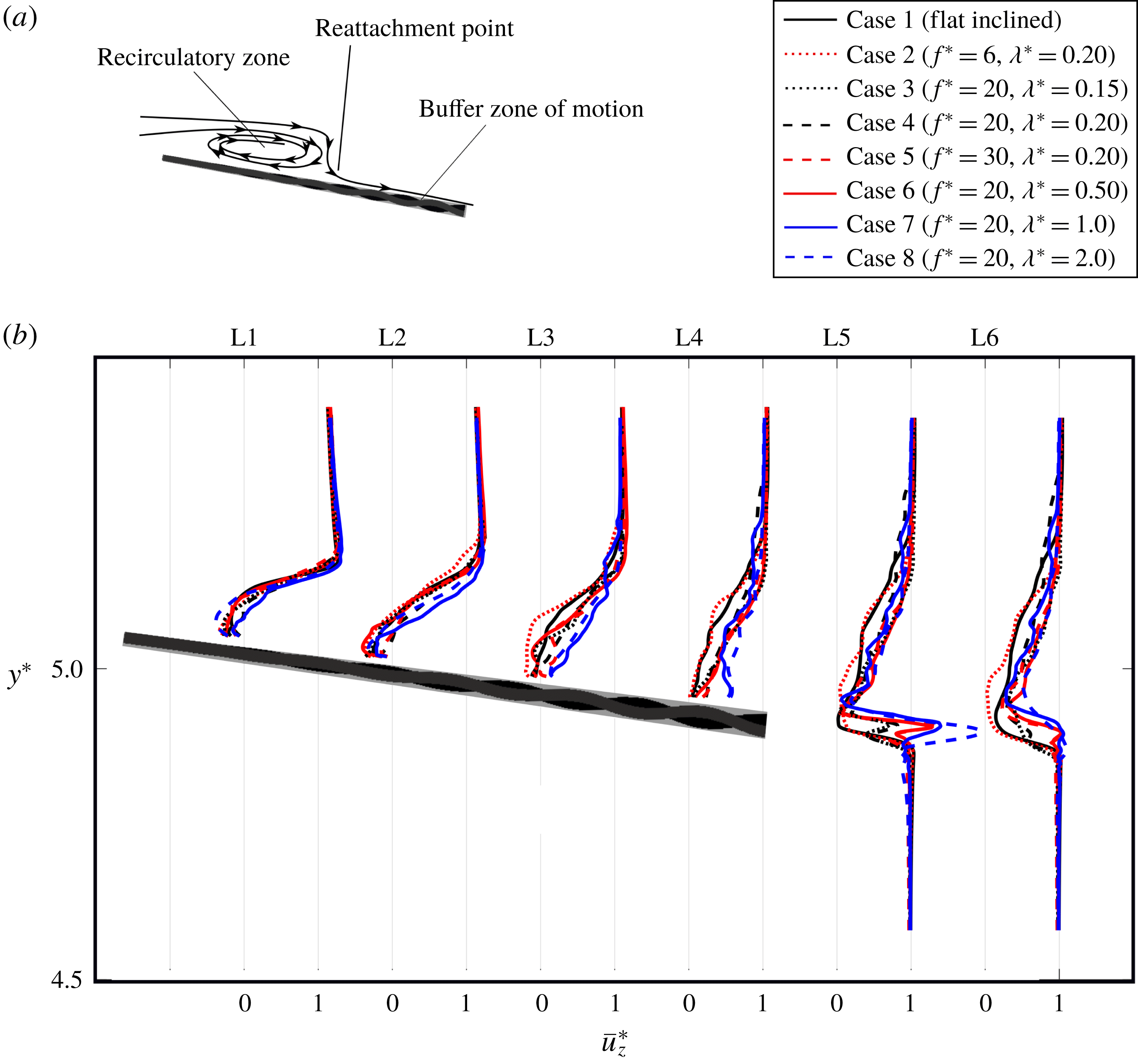
) on the midplane. For oscillating plates, the reattachment point is found over the buffer zone of motion, which contains all the points that the moving plate has passed through at least once in a cycle. This buffer zone is shown schematically by the grey region in figure 4(a). This buffer zone is defined because the time averaging of values, e.g. velocities, is valid only for the fluid nodes and not the solid nodes. Therefore, the time-averaged values in this study, including the pressure and velocity values, are for the nodes that are out of this buffer zone. The reattachment point can be visually detected by the streamline normal to the plate, as shown schematically in figure 4(a). The exact reattachment length, denoted by
 $R$
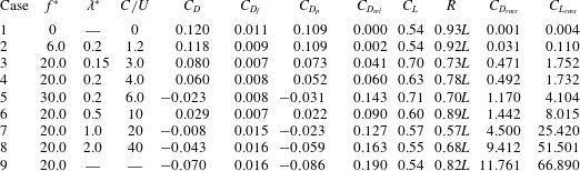
, is reported in table 2.
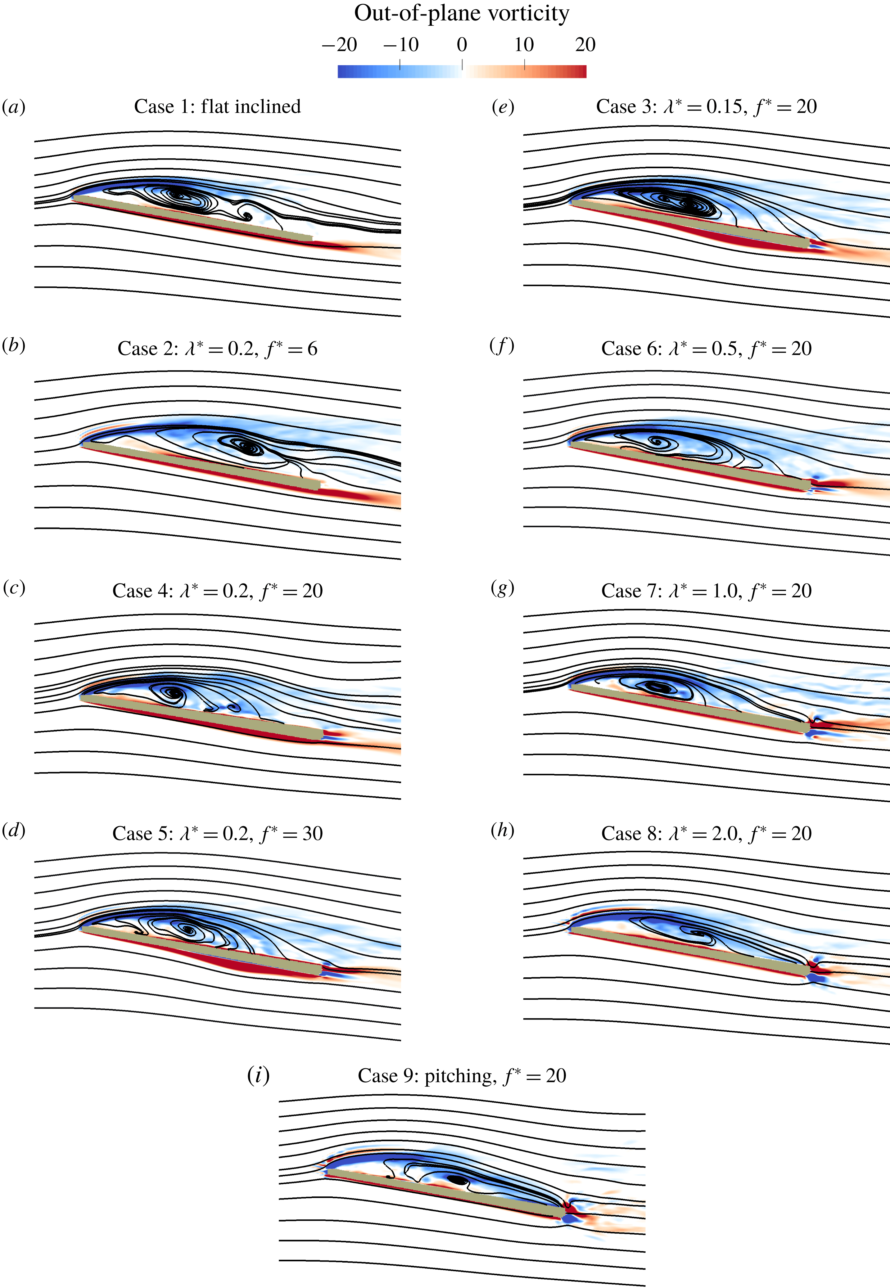
Out-of-plane vorticity contours and streamlines of the mean flow on the midplane for nine cases. The left and right columns show the effect of frequency and wavelength on flow separation, respectively.

Values of the mean drag coefficient
 $(C_{D})$
, relative drag coefficient
 $(C_{D_{rel}})$
, viscous drag
 $(C_{D_{f}})$
, form drag
 $(C_{D_{p}})$
, relative drag
 $(C_{D_{rel}})$
, lift coefficient
 $(C_{L})$
, reattachment length (
 $R$
) and the r.m.s. values of drag and lift coefficients for different cases. The relative drag
 $(C_{D_{rel}})$
is defined as the drag reduction relative to case 1 (flat inclined) along the plate chord (
 $C_{D_{rel}}=(C_{D}^{flat\,inclined}-C_{D}^{undulating})/\cos \unicode[STIX]{x1D703}$
), which is a measure of the thrust force produced by the wave. All force coefficients are non-dimensionalized with
 $\unicode[STIX]{x1D70C}U^{2}L^{2}$
, as the area of the plate is
 $2L^{2}$
. Case 1 is the non-moving flat inclined plate and case 9 is the pitching inclined plate, for which the wave speed is not defined.

To visualize the flow separation, the time-averaged streamlines and out-of-plane vorticity on the midplane of the nine cases (table 2) are presented in figure 3. Figure 3(a–d) shows the cases with similar wavelength but different frequency, i.e. the effect of frequency, while figure 3(e–h) shows the cases with similar frequency but different wavelength, i.e. the effect of wavelength. Owing to the sharp leading edge of the plate, the flow separates from the leading edge for all cases and forms a clockwise recirculatory region near the leading edge (figure 3), which is depicted schematically in figure 4(a). This recirculatory (separation) region is represented by the negative (clockwise) vorticity (figure 3).
Over the flat inclined plate (figure 3
a), the separated shear layer, which is inviscidly unstable, transitions to turbulence and reattaches near the trailing edge (
 $0.93L$
) as the turbulent flow energizes the near-wall flow (Mueller & Batil Reference Mueller and Batil1982). The travelling wave at low frequency
 $f^{\ast }=6$
does not affect the flow separation (figure 3
b) and the reattachment length is similar to that for the flat inclined plate (table 2). By increasing
 $f^{\ast }$
from 6 to 20 and 30 (
 $C/U$
from 1.2 to 4 and 6), however, the separated shear layer reattaches earlier at
 $0.78L$
and
 $0.70L$
from the leading edge (table 2), respectively, as observed in figure 3(c,d). In fact, comparing the streamlines in the left column of figure 3 shows that increasing the wave speed by increasing the frequency in this range reduces flow separation monotonically.
(a) Schematic of the average flow field. The grey zone is the buffer zone of the motion, which includes all points the plate passes through at least once in a cycle. (b) The non-dimensional time-averaged streamwise velocity profile
 $\overline{u_{z}^{\ast }}$
at midplane.

The wavelength variation at constant frequency did not produce a monotonic pattern for decrease/increase of the flow separation (figure 3
e–h). Increasing
 $\unicode[STIX]{x1D706}^{\ast }$
from 0.15 (case 3) to 0.2 (case 4) and 0.5 (case 6) at constant
 $f^{\ast }=20$
, i.e. increasing
 $C/U$
from 3 to 4 and 10, increases the separation length from
 $0.73L$
to
 $0.78L$
and
 $0.89L$
, respectively (table 2 and compare figure 3
e, c and f). By increasing the wavelength further from 0.5 (case 6) to 1.0 (case 7) and 2.0 (case 8) (
 $C/U$
from 10 to 20 and 40), however, the reattachment length reduces to
 $0.57L$
and then increases to
 $0.68L$
(table 2), respectively, as observed in figure 3(f–h). For the pitching plate (case 9), the flow separation increases compared to case 8 (
 $\unicode[STIX]{x1D706}^{\ast }=2.0$
), i.e. reattachment length increases to
 $0.82L$
(table 2 and figure 3
h,i). In summary, when the wave speed increases by increasing the wavelength (figure 3
e–h), in contrast to the trend observed for frequency (figure 3
a–d), the flow reattachment length neither decreases nor increases monotonically.
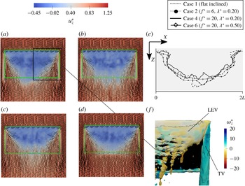
Streamwise velocity field over the plane adjacent to the top surface of the buffer zone of the motion: (a) flat inclined plate, (b) undulating plate case 2 (
 $f^{\ast }=6$
,
 $\unicode[STIX]{x1D706}^{\ast }=0.2$
), (c) undulating plate case 4 (
 $f^{\ast }=20$
,
 $\unicode[STIX]{x1D706}^{\ast }=0.2$
) and (d) undulating plate case 6 (
 $f^{\ast }=20$
,
 $\unicode[STIX]{x1D706}^{\ast }=0.5$
). The green rectangle is the plate. (e) The corresponding reattachment line plotted along the span of the plate by detecting the zero streamwise velocity for these cases. Here
 $x=0$
and
 $x=2L$
are tips, and
 $x=L$
is the midplane of the plate. (f) Time-averaged vortices on the suction side, including LEV and tip vortex (TV) identified by
 $Q$
-criterion with
 $Q=10$
and coloured with non-dimensional streamwise vorticity (
 $\unicode[STIX]{x1D714}_{z}^{\ast }$
).

To clearly show the reattaching and reverse flows, figure 4(b) presents the time-averaged streamwise velocity profile at six sections on the midplane. The time-averaged streamwise velocity profile of cases 1 and 2 are approximately identical in all sections of figure 4(b), which agrees with the results of table 2, indicating that low
 $f^{\ast }$
(case 2) does not change the reattachment length compared to the flat inclined one (case 1). As
 $f^{\ast }$
increases to 20, the reverse flow increases slightly near the leading edge, in sections L1 and L2 of figure 4(b), for cases 6 and 8, whereas it decreases in section L2 for case 7, which has the minimum reattachment length (table 2). Near the trailing edge, at section L4 of figure 4(b), the time-averaged streamwise velocity of cases 3–8 is higher than for cases 1 and 2 as the flow has reattached earlier for cases 3–8 (table 2).
To investigate the flow reattachment at different spanwise locations, the time-averaged streamwise velocity field on the plane that is adjacent to the top surface of the buffer zone of the motion is shown for cases 1, 2, 4 and 6 in figure 5(a–d). The velocity vectors in figure 5(a–d) are the projected velocity field to this plane. It can be observed in figure 5(a–d) that the reverse flow is higher near the midplane (
 $x=L$
) for all cases and decreases towards the tips of the plate as the spanwise velocity increases. Figure 5(e) shows the reattachment lines of cases 1, 2, 4 and 6, which are plotted by detecting the boundary of zero streamwise velocity of figure 5(a–d), and the time-averaged tip vortex (TV) and LEV of the flat inclined plate are visualized using the
 $Q$
-criterion in figure 5(f). The profile of the reattachment length (figure 5
e) shows that the flow reattaches earlier as we move towards the tips from the midplane due to the impact of the tip vortex. The tip vortex, which has a higher streamwise vorticity compared to the LEV, induces a spanwise velocity near the tips (figure 5
a–d), which contributes to the earlier flow reattachment near the tips of the plate (Kim & Gharib Reference Kim and Gharib2010).
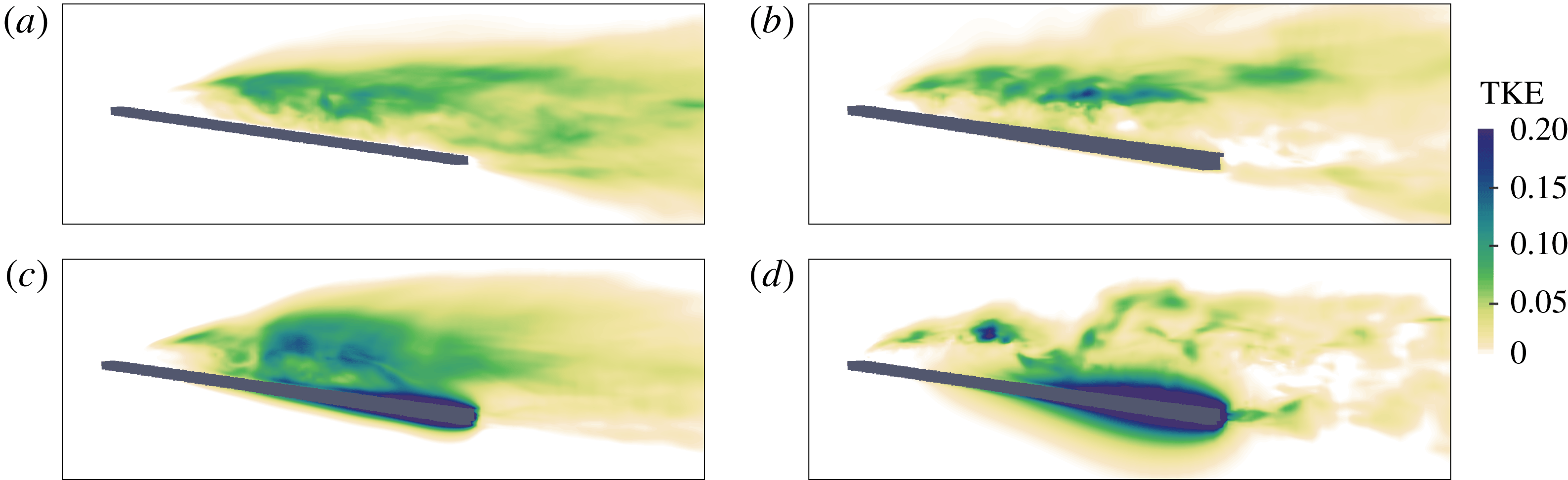
Distribution of the non-dimensional turbulent kinetic energy in (a) flat inclined plate, (b) undulating plate case 2 (
 $f^{\ast }=6$
,
 $\unicode[STIX]{x1D706}^{\ast }=0.2$
), (c) undulating plate case 4 (
 $f^{\ast }=20$
,
 $\unicode[STIX]{x1D706}^{\ast }=0.2$
) and (d) undulating plate case 6 (
 $f^{\ast }=20$
,
 $\unicode[STIX]{x1D706}^{\ast }=0.5$
). The undulations increase the TKE over the plate, but decrease it in the wake downstream of the trailing edge.

3.2 The effect of travelling waves on turbulence intensity
Travelling waves are known to reduce the turbulence intensity of turbulent boundary layers, e.g. turbulent channel flows (Shen et al. Reference Shen, Zhang, Yue and Triantafyllou2003; Nakanishi, Mamori & Fukagata Reference Nakanishi, Mamori and Fukagata2012; Mamori, Iwamoto & Murata Reference Mamori, Iwamoto and Murata2014), by decreasing the random component of the flow (Mamori et al. Reference Mamori, Iwamoto and Murata2014). However, the effect of travelling waves on the turbulent intensity in external flows, e.g. flow over an inclined plate, where the boundary layer is not fully turbulent, is unknown. Here, we investigate the effect of travelling waves on the turbulence intensity of the flow.
To investigate the effects of travelling waves on turbulence intensity, the turbulent kinetic energy (TKE) is shown for cases 1, 2, 4 and 6 in figure 6(a–d), respectively. The TKE of the flat inclined plate is non-zero on the plate’s suction side where the separated shear layer mixes with reverse flow near the wall, but zero on the pressure side. Similarly, the TKE is non-zero only on the suction side of the low-frequency case (case 2) (figure 6
b). The TKE of the flow adjacent to both sides of the undulating plate increases as
 $f^{\ast }$
and
 $\unicode[STIX]{x1D706}^{\ast }$
increase (figure 6
c,d). However, in case 4, which has the lowest reattachment length among these cases, the TKE over the plate at the separation zone is higher than in other cases (figure 6
c). In addition, the TKE is lower in the wake downstream of the plate for cases 4 and 6 compared to the flat inclined plate.
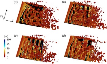
Three-dimensional vortical structures visualized by the instantaneous isosurfaces of the
 $Q$
-criterion (
 $Q=20$
) from midplane to the tip. (a) Flat inclined plate, (b) undulating plate case 2 (
 $f^{\ast }=6$
,
 $\unicode[STIX]{x1D706}^{\ast }=0.2$
), (c) undulating plate case 4 (
 $f^{\ast }=20$
,
 $\unicode[STIX]{x1D706}^{\ast }=0.2$
) and (d) undulating plate case 6 (
 $f^{\ast }=20$
,
 $\unicode[STIX]{x1D706}^{\ast }=0.5$
).

The decrease of TKE in the downstream wake for high-frequency undulatory cases (figure 6
c,d) can also be observed by the instantaneous 3-D vortical structures. Figure 7 shows the 3-D vortical structures visualized by the isosurface of the
 $Q$
-criterion. Comparing the wake of cases 4 and 6 with the flat inclined one (figure 7
a,c,d) reveals that the number of vortical structures have decreased for cases 4 and 6 compared to case 1, which confirms the decrease of turbulence intensity in the wake (figure 6
a,c,d). Furthermore, it can be observed that the shear layer separates from the sharp leading edge and breaks down into small vortices as it becomes unstable. The vortical structures of the flat inclined plate resemble the vortices visualized by Visbal (Reference Visbal2011) whose plate had the same aspect ratio (
 $=2$
) but the angle of attack was
 $8^{\circ }$
. It can also be observed that the flow is more spread laterally at the midplane compared to the regions near the tips of the plate.
3.3 The effect of travelling waves on the aerodynamic performance
The flow visualizations in the previous section showed that travelling waves can reduce flow separation, which can impact both the drag and lift forces. A reduction in drag force is expected because backward travelling waves are known to generate thrust, which propels aquatic swimmers forwards (Lighthill Reference Lighthill1960; Fish & Lauder Reference Fish and Lauder2006; Borazjani & Sotiropoulos Reference Borazjani and Sotiropoulos2010). However, the effect of travelling waves on the lift coefficient cannot be predicted purely based on the thrust generation because travelling waves completely change the pressure field by creating a low-pressure region on both sides of the plate at high frequencies, as will be discussed below. In addition, the effects of travelling waves on the mean and instantaneous aerodynamic forces are discussed by comparing the trend of computed forces and the analytically derived ones using EBT (Lighthill Reference Lighthill1960).
To quantify the aerodynamic performance, the drag (
 $C_{D}$
), relative drag (
 $C_{D_{rel}}$
) and lift (
 $C_{L}$
) coefficients, and the r.m.s. values of fluctuations of drag and lift coefficients, are reported in table 2. The drag coefficient (
 $C_{D}=F_{drag}/(\unicode[STIX]{x1D70C}U^{2}L^{2})$
) is the total non-dimensional drag force, which consists of the viscous (
 $C_{D_{f}}$
) and form (
 $C_{D_{p}}$
) drag acting on the plate along the incoming flow (
 $z$
direction); and the lift coefficient (
 $C_{L}=F_{lift}/(\unicode[STIX]{x1D70C}U^{2}L^{2})$
) is the total non-dimensional force acting normal to the incoming flow in the
 $y$
direction. The relative drag coefficient for each case is defined as the drag reduction relative to the flat inclined case along the plate (
 $C_{D_{rel}}=(C_{D}^{flat\,inclined}-C_{D}^{undulating})/\cos \unicode[STIX]{x1D703}$
), which is almost equivalent to the thrust force produced by the oscillations. The time-averaged results for the oscillating plates are averaged over 60 cycles and the averaging is started after 50 cycles.
Table 2 shows that the viscous drag is approximately 10 % of the form (pressure) drag. When the plate undulates at a high reduced frequency
 $(f^{\ast }\geqslant 20)$
, e.g. cases 3–8, the ratio of the viscous to the form drag increases because the form drag is reduced by the undulations (undulations generate thrust) while viscous drag is negligibly changed. In fact, the change in the viscous drag with respect to the flat inclined plate is less than 0.005 for all cases (
 $|\unicode[STIX]{x0394}C_{D_{f}}|<0.005$
, where
 $\unicode[STIX]{x0394}C_{D_{f}}=C_{D_{f}}^{flat\,inclined}-C_{D_{f}}^{undulating}$
is the difference between the viscous drag of the flat inclined plate and an undulating one). Consequently, the reduction in form drag accounts for the majority of the reduction in drag coefficient (
 $C_{D}$
).
Comparing the time-averaged values, table 2 shows that in case 2 (
 $f^{\ast }=6$
,
 $C/U=1.2$
) the travelling wave does not improve the aerodynamic performance compared to the flat inclined plate. However, increasing the wave speed by increasing the reduced frequency to
 $f^{\ast }=20$
(
 $C/U=4$
) and
 $f^{\ast }=30$
(
 $C/U=6$
) increases the lift force by 16.7 % and 31.4 % and decreases the drag force by 50 % and 119.2 % (generates thrust), respectively. It is interesting to note that when the travelling wave generates thrust (positive relative drag in table 2) at high
 $f^{\ast }$
, e.g. cases 3–8, a jet-like profile velocity is observed in the wake (sections L5 of figure 4
b). In addition, the thrust produced in cases 5, 7, 8 and 9 is high, such that the drag (
 $C_{D}$
) is negative (thrust type). In these cases a streamwise flow can be observed in the middle of the plate (section L3 of figure 4
b), i.e. jet-like profile is initiated earlier (closer to the leading edge).
When the frequency is kept the same (
 $f^{\ast }=20$
), increasing the wave speed by increasing the wavelength from
 $\unicode[STIX]{x1D706}^{\ast }=0.15$
(
 $C/U=3$
) in case 3 to
 $\unicode[STIX]{x1D706}^{\ast }=0.2$
(
 $C/U=4$
) in case 4 decreases the lift by 10 % (case 3 is 29 % higher than the flat inclined plate) but increases the relative drag by 33 %. Similarly, when the wave speed is further increased by increasing the wavelength to 0.5 in case 6 (
 $f^{\ast }=20$
,
 $C/U=10$
), lift decreases but thrust (relative drag) increases compared to case 4. Nevertheless,
 $C_{L}$
is still 9.2 % higher than the lift of the flat inclined plate. Similar results such as the increase of thrust (relative drag) and the decrease of lift are observed by increasing the wavelength to 1.0 and 2.0 in cases 7 and 8, respectively. It can also be observed that the pitching motion (case 9) produces the maximum relative drag but it does not change the lift compared to the flat inclined case.
Theoretically, the time-averaged thrust (relative drag) increases with both frequency and wavelength as wave speed
 $C$
increases according to EBT (Lighthill Reference Lighthill1960) – see appendix C for the derivation:
 $$\begin{eqnarray}C_{T}=0.11\unicode[STIX]{x03C0}(2\unicode[STIX]{x03C0}f^{\ast }a_{max}^{\ast })^{2}\left(1-\left(\frac{1}{\unicode[STIX]{x1D706}^{\ast }f^{\ast }}\right)^{2}\right).\end{eqnarray}$$
Note that
 $1/(\unicode[STIX]{x1D706}^{\ast }f^{\ast })=U/C$
. The calculated relative drag (table 2) follows the trend predicted by EBT, i.e. the thrust (relative drag) increases with increasing wave speed through increasing
 $f^{\ast }$
and/or
 $\unicode[STIX]{x1D706}^{\ast }$
. However, the lift force does not follow the same trend.
(a) Spanwise-averaged distribution of the lift coefficient along the plate with three points along the span of the plate. The symbols ○, ▪ and
 $+$
are the lift coefficient at
 $0.3L$
,
 $L$
(midplane) and
 $0.1L$
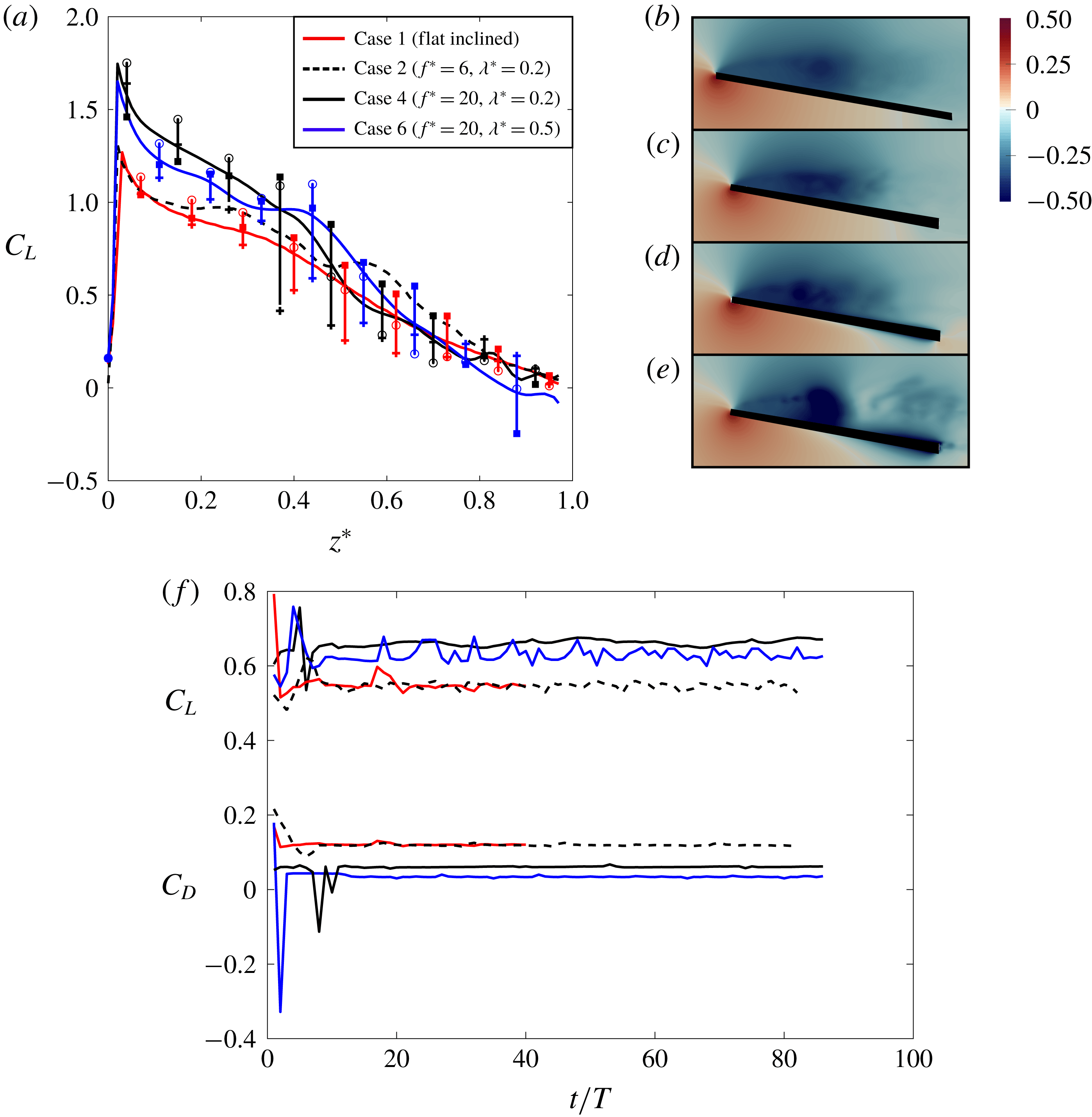
from the tip of the plate, respectively, for cases 1, 4 and 6. (b–e) Time-averaged pressure field at midplane for cases 1, 2, 4 and 6, respectively. (f) Time history of cycle-averaged lift (upper curve) and drag coefficient (lower curve), for cases 2, 4 and 6. Here,
 $T$
is the period of the wave for undulating cases, which is
 $1/f$
, and
 $T$
is defined as
 $T=L/U$
for the flat inclined plate.

The lift force of cases 3–7 (undulating at high
 $f^{\ast }$
) has increased compared to the flat inclined plate (case 1) as observed in table 2. A simple explanation is that the travelling waves on the plates generate thrust along the
 $Z$
direction (figure 1
b), which has a component in the lift (
 $y$
) direction, i.e. enhances lift. The contribution of thrust force, generated by travelling waves, to the lift coefficient (denoted by
 $\unicode[STIX]{x0394}C_{L}$
here) can be approximated by the component of the thrust force in the lift (
 $y$
) direction, i.e.
 $\unicode[STIX]{x0394}C_{L}=C_{T}\sin \unicode[STIX]{x1D703}$
, where
 $\unicode[STIX]{x1D703}$
is the angle of attack (the angle between
 $Z$
and
 $z$
directions in figure 1). Therefore, for case 3,
 $\unicode[STIX]{x0394}C_{L}=0.06\times \sin (10^{\circ })\approx 0.005$
. This is two orders of magnitude smaller than the lift enhancement of cases 3–6 (
 ${\approx}0.1$
) relative to the flat inclined plate (table 2). Therefore, the
 $z$
component of the generated thrust is not the main reason for such lift enhancement. The lift enhancement is due to the modification of the pressure distribution around the plate, which is further investigated below.
To see how the lift force along the plate is modified by the travelling waves, the mean spanwise-averaged lift distribution along the plate for the flat inclined plate and three undulating cases (2, 4 and 6) is presented in figure 8(a). To see the spatial dependence of the lift force, the spanwise averages are shown along with the lift coefficient at three sections across the span of the plate,
 $X=0.1L$
,
 $X=0.3L$
and
 $X=L$
, where
 $X$
is the spanwise distance between the section and the tip of the plate (see figure 5
e). It can be observed that the range of spanwise variation of the lift is higher in the recirculatory (separated) zone (see the error bars (vertical lines) in figure 8
a) because the lift is high on the midplane but decreases more near the tips of the plate (
 $X=0.1L$
) due to the tip vortex (figure 5
f) (Kim & Gharib Reference Kim and Gharib2010; Beem et al.
Reference Beem, Rival and Triantafyllou2012). In addition, it can be observed that these variations are higher for the undulating cases.
To show that the lift force along the plate has reached quasi-steady state, the time histories of the cycle-averaged lift and drag coefficients for flat inclined (case 1) and three undulating cases (2, 4 and 6) are shown in (figure 8
f). Figure 8(f) shows that the cycle-averaged forces for undulating cases become steady after approximately 12 cycles. The lift forces of undulating cases 2, 4 and 6 plotted in figure 8(a) are averaged over 20 cycles, and averaging is started after 50 cycles, as the forces are steady as shown in figure 8(f). The time averaging for the flat inclined plate is performed for
 $10t/T$
, which is equivalent to 4000 iterations.
Comparing the mean spanwise-averaged lift coefficient of undulating plates with the flat inclined one (figure 8
a) shows that
 $C_{L}$
does not change significantly for the low-frequency undulating case (case 2), but it becomes higher near the leading edge and slightly decreases near the trailing edge for high-frequency undulatory cases. This indicates that the total lift of cases 4 and 6 has increased compared to the lift of the flat inclined plate (case 1) due to the increase of the generated lift near the leading edge. In fact, case 4, which has the largest
 $C_{L}$
near the leading edge (figure 8
a), has the highest total lift coefficient among these four cases (table 2).
The lift of high-
 $f^{\ast }$
cases (4 and 6) has increased near the leading edge because of the lower pressure in the recirculatory zone relative to the pressure side (figure 8
d,e). The reason for the slightly lower lift coefficient of the high-
 $f^{\ast }$
cases in the vicinity of the trailing edge (figure 8
a) is the symmetric time-averaged pressure distribution (figure 8
d,e). It can be observed in figure 8(d,e) that a low pressure exists on both suction and pressure sides of the undulating plate near the trailing-edge area, which can be explained by the scaling of pressure on an undulating surface at high frequency. The pressure on an undulating inclined plate is generated by two mechanisms: (i) the angle of the plate, which pushes the incoming flow downwards (downwash), generating a higher pressure on the lower surface and a lower pressure on the upper surface; and (ii) the pressure created by the undulations of the plate, which accelerates the fluid near the plate (appendix D). The pressure due to undulations (undulating pressure) increases as frequency increases. In fact, for the undulating pressure, the normal component of the time-averaged pressure gradient along the lateral direction pointing outwards from the plate
 $\unicode[STIX]{x2202}\bar{p}/\unicode[STIX]{x2202}n$
, near the trailing edge, scales with
 $(a_{max}^{\ast })^{2}(f^{\ast }-1/\unicode[STIX]{x1D706}^{\ast })^{2}$
, which is derived by simplifying the time-averaged Navier–Stokes equations (see appendix D). Note that the positive
 $\unicode[STIX]{x2202}\bar{p}/\unicode[STIX]{x2202}n$
indicates that the pressure increases as we move away from the plate in the normal direction, i.e. a low pressure near the undulating plate. At high frequencies (cases 3–8), the undulating component dominates the pressure created by downwash (flat inclined plate). In fact, the magnitude of pressure near the trailing edge of an undulating plate at higher frequencies is one order of magnitude larger than the pressure over the trailing edge of the flat inclined plate (case 1). Therefore, the pressure near the trailing edge on both sides of the plate becomes similar at high
 $f^{\ast }$
, i.e. results in a low symmetric time-averaged pressure distribution (figure 8
d,e), because (i) the pressure at the trailing edge is dominated by the undulating pressure at high
 $f^{\ast }$
and (ii) the undulating pressure is similar (low) on both sides of the plate.
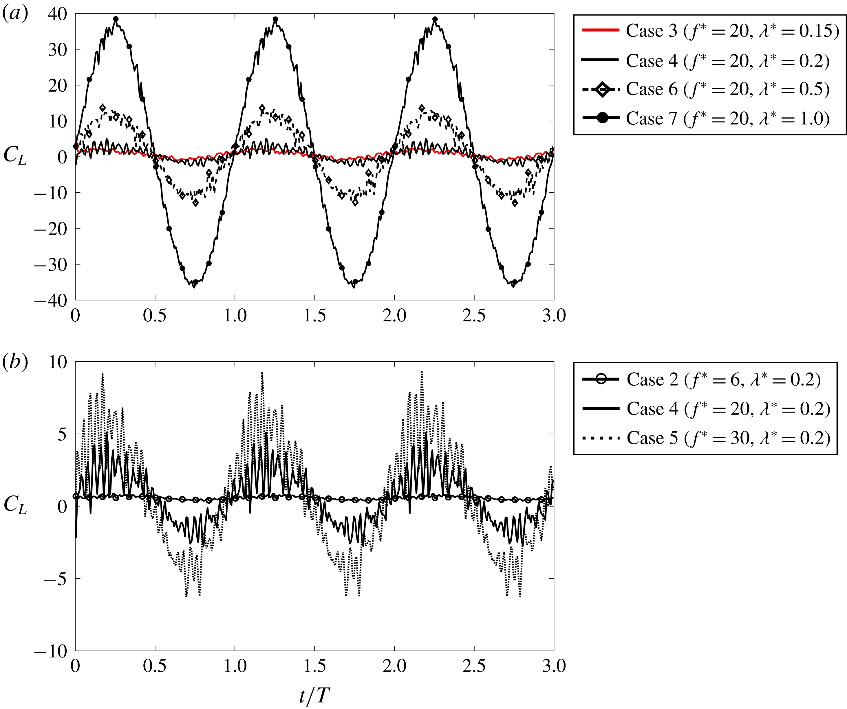
(a) The effect of wavelength on the instantaneous lift coefficient. Instantaneous lift coefficients for three cycles at quasi-steady state for four oscillating cases with the same
 $f^{\ast }=20$
: case 3 (
 $f^{\ast }=20$
,
 $\unicode[STIX]{x1D706}^{\ast }=0.15$
), case 4 (
 $f^{\ast }=20$
,
 $\unicode[STIX]{x1D706}^{\ast }=0.2$
), case 6 (
 $f^{\ast }=20$
,
 $\unicode[STIX]{x1D706}^{\ast }=0.5$
) and case 7 (
 $f^{\ast }=20$
,
 $\unicode[STIX]{x1D706}^{\ast }=1.0$
). (b) The effect of frequency on the instantaneous lift coefficient. Instantaneous lift coefficient for three cycles at quasi-steady state for three undulating cases with the same
 $\unicode[STIX]{x1D706}^{\ast }=0.2$
and different
 $f^{\ast }$
: case 2 (
 $f^{\ast }=6$
,
 $\unicode[STIX]{x1D706}^{\ast }=0.2$
), case 4 (
 $f^{\ast }=20$
,
 $\unicode[STIX]{x1D706}^{\ast }=0.2$
) and case 5 (
 $f^{\ast }=30$
,
 $\unicode[STIX]{x1D706}^{\ast }=0.2$
). Here,
 $T=1/f$
is the period of the wave for undulating cases.

Although EBT does not predict any mean lift generation when the plate is undergoing an undulatory oscillation, it predicts a sinusoidal profile for instantaneous lift and thrust, similar to aquatic swimmers (Triantafyllou et al.
Reference Triantafyllou, Triantafyllou and Yue2000; Borazjani & Sotiropoulos Reference Borazjani and Sotiropoulos2009), which increases the r.m.s. value of the forces. The r.m.s. values of lift and drag coefficients are presented in table 2. It can be observed that the r.m.s. values for fluctuations of both lift and drag coefficients are small for the flat inclined plate (
 $C_{L_{rms}}=0.004,~C_{D_{rms}}=0.001$
). When the plate undulates with a low frequency (case 2,
 $f^{\ast }=6$
,
 $\unicode[STIX]{x1D706}^{\ast }=0.2$
), the r.m.s. values increase compared to the flat inclined plate, but the r.m.s. values are still less than the mean values (
 $C_{L_{rms}}/C_{L}\approx 0.2$
and
 $C_{D_{rms}}/C_{D}\approx 0.25$
). By increasing the reduced frequency, however, in case 4 (
 $f^{\ast }=20$
,
 $\unicode[STIX]{x1D706}^{\ast }=0.2$
),
 $C_{L_{rms}}/C_{L}$
and
 $C_{D_{rms}}/C_{D}$
increase approximately to 3 and 6, respectively. It can be observed that, when the wavelength increases, the r.m.s. values increase more intensely, e.g. in case 6 (
 $f^{\ast }=20$
,
 $\unicode[STIX]{x1D706}=0.5$
)
 $C_{L_{rms}}/C_{L}$
increases to 50. The high r.m.s. values of the forces in high-frequency oscillating cases 3–9 can be explained by the instantaneous forces. The effect of
 $\unicode[STIX]{x1D706}^{\ast }$
and
 $f^{\ast }$
on the instantaneous lift coefficient after reaching quasi-steady state is shown in figure 9(a) and 9(b), respectively. When the frequency increases, the intensity of the fluctuations increases (figure 9
b) and consequently the r.m.s. value of the forces increases as well (table 2). Increasing the wavelength, however, increases the amplitude of the forces more intensely (figure 9
a), e.g. the amplitude of the lateral force has increased from 14 to 37 by increasing the wavelength from 0.5 to 1.0. It can be noted that, although the net reduced drag generated by the wave is higher for case 5 than for cases 6 and 7 (table 2), the amplitude of the fluctuation is higher for cases 6 and 7. The observed trends are consistent with the theoretical trend for the amplitude of instantaneous lateral (reactive) force, according to EBT (Lighthill Reference Lighthill1960). In fact, the amplitude of the lateral force of an undulating plate scales with
 $O(\unicode[STIX]{x1D706}^{\ast }(f^{\ast }-1/\unicode[STIX]{x1D706}^{\ast })^{2})$
, according to (C 6) derived in appendix C.
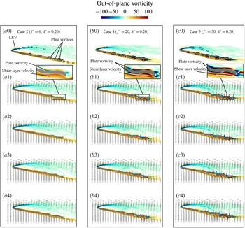
The effect of frequency on the phase-averaged flow field of undulating cases with similar wavelength (
 $\unicode[STIX]{x1D706}^{\ast }=0.2$
) on the midplane. The first row for each case visualizes the contours of out-of-plane vorticity and the footprint of the
 $Q$
-criterion (
 $Q=40$
) by black lines for phase angle
 $t/T=0$
. The second to fifth rows for each case visualize the vorticity and velocity vectors of the flow close to the plate for four phase angles. (a0–a4) The undulating plate case 2 (
 $f^{\ast }=6$
,
 $\unicode[STIX]{x1D706}^{\ast }=0.2$
), (b0–b4) the undulating plate case 4 (
 $f^{\ast }=20$
,
 $\unicode[STIX]{x1D706}^{\ast }=0.2$
) and (c0–c4) the undulating plate case 5 (
 $f^{\ast }=30$
,
 $\unicode[STIX]{x1D706}^{\ast }=0.5$
). The inset shows the shear layer vorticity over the pressure side, and the plate vorticity over the pressure and suction sides of the plate. The visualizations of the second to fifth rows of each case are for phase angle of (1)
 $t/T=0.0$
, (2)
 $t/T=0.25$
, (3)
 $t/T=0.5$
and (4)
 $t/T=0.75$
, respectively; and
 $T=1/f$
is the period of each case.

The effect of wavelength on the phase-averaged flow field of undulating cases with similar frequency (
 $f^{\ast }=20$
) on the midplane. The first row for each case visualizes the contours of out-of-plane vorticity and the footprint of the
 $Q$
-criterion (
 $Q=40$
) by black lines for phase angle
 $t/T=0$
. The second to fifth rows for each case visualize the vorticity and velocity vectors of flow close to the plate for four phase angles. (a0–a4) The undulating plate case 6 (
 $f^{\ast }=20$
,
 $\unicode[STIX]{x1D706}^{\ast }=0.5$
), (b0–b4) the undulating plate case 7 (
 $f^{\ast }=20$
,
 $\unicode[STIX]{x1D706}^{\ast }=1.0$
) and (c0–c4) the undulating plate case 8 (
 $f^{\ast }=20$
,
 $\unicode[STIX]{x1D706}^{\ast }=2.0$
). The inset shows the shear layer vorticity over the pressure side, and the plate vorticity over the pressure and suction sides of the plate. The visualizations of the second to fifth rows of each case are for phase angle of (1)
 $t/T=0.0$
, (2)
 $t/T=0.25$
, (3)
 $t/T=0.5$
and (4)
 $t/T=0.75$
, respectively; and
 $T=1/f$
is the period of each case.

3.4 Travelling waves and the mechanisms of flow reattachment
Travelling waves were shown to reduce turbulence intensity in the wake but increase it near the plate (§ 3.2). In addition, they were shown to reduce flow separation of the mean flow at high frequency while the wavelength effect was not monotonic (§ 3.1). To explain the effect of wave parameters on turbulence intensity, reattachment and detachment of the flow, the phase-averaged flow along with their corresponding scalings, e.g. lateral velocity (
 $u_{Y}$
), are investigated in this section, which will reveal the main mechanisms governing flow reattachment by travelling waves.
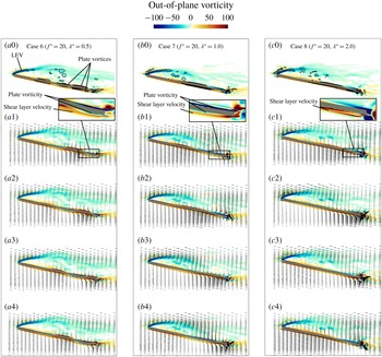
Figures 10 and 11 represent the effect of frequency and wavelength, respectively, on the phase-averaged flow field visualized by out-of-plane vorticity and velocity vectors for four phase angles. The first row of each case (figures 10 and 11) shows the contours of vorticity and the footprints of the 3-D vortices identified by the isolines of the
 $Q$
-criterion for the first phase angle (
 $t/T=0$
). The four rows below it show the velocity vectors and vorticity contours near the plate at four other time instants in the cycle. In all cases, an attached and a separated shear layer are formed on the pressure and suction sides of the plate, respectively. The shear layer on the suction side, which has been separated at the leading edge, forms an LEV that sheds into the wake.
In addition to the vortices shed to the wake by the LEV, there are vortices on the plate that travel by the travelling wave along the plate and into the wake (see figure 10
a0). The vorticity of these vortices (the non-dimensional out-of-plane vorticity of the fluid on the plate) is composed of the plate vorticity (
 $\unicode[STIX]{x2202}u_{Y}^{\ast }/\unicode[STIX]{x2202}Z^{\ast }$
) and the shear layer vorticity (
 $\unicode[STIX]{x2202}u_{Z}^{\ast }/\unicode[STIX]{x2202}Y^{\ast }$
), i.e.
 $\text{out-of-plane vorticity}=-\text{in-plane vorticity}=-\unicode[STIX]{x1D714}_{x}^{\ast }=-(\unicode[STIX]{x2202}u_{Y}^{\ast }/\unicode[STIX]{x2202}Z^{\ast }-\unicode[STIX]{x2202}u_{Z}^{\ast }/\unicode[STIX]{x2202}Y^{\ast })$
. The plate vorticity is obtained by taking the derivative of the lateral velocity with respect to the streamwise length (
 $\unicode[STIX]{x2202}u_{Y}^{\ast }/\unicode[STIX]{x2202}Z^{\ast }$
) because the plate has no streamwise motion (
 $u_{Z}=0$
). The plate vorticity scales with
 $O((a_{max}^{\ast }/\unicode[STIX]{x1D706}^{\ast })(f^{\ast }-1/\unicode[STIX]{x1D706}^{\ast }))$
while the shear layer vorticity scales with
 $O(\sqrt{Re})$
for an attached boundary layer of the plate based on Blasius skin-friction coefficient (Schlichting & Gersten Reference Schlichting and Gersten2016) – see appendix C.
If the flow is separated, e.g. on the suction side, the shear layer vorticity is low and the plate vorticity dominates. Consequently, the vorticity of the fluid near the plate follows the same trend as the plate vorticity on the suction side as observed in figures 10 and 11, e.g. the vorticity on the suction side is anticlockwise (positive) and clockwise (negative) on the peaks and valleys of the wave, respectively, similar to the plate vorticity for all cases (figures 10 and 11). On the pressure side, however, the shear layer is attached and creates an anticlockwise (positive) vorticity. The shear layer vorticity is approximately
 $0.3\sqrt{Re}\approx 45$
, which is much higher than the plate vorticity at low frequency (case 2), which is approximately
 $4\unicode[STIX]{x03C0}^{2}(a_{max}^{\ast }/\unicode[STIX]{x1D706}^{\ast })(f^{\ast }-1/\unicode[STIX]{x1D706}^{\ast })\approx 2$
. Similarly, for case 8, which has a high wavelength (
 $\unicode[STIX]{x1D706}^{\ast }$
), the approximation of plate vorticity
 $(\unicode[STIX]{x2202}u_{Y}^{\ast }/\unicode[STIX]{x2202}Z^{\ast }\approx 4\unicode[STIX]{x03C0}^{2}(a_{max}^{\ast }/\unicode[STIX]{x1D706}^{\ast })(f^{\ast }-1/\unicode[STIX]{x1D706}^{\ast })\approx 5)$
is much smaller than the shear layer vorticity
 $(\unicode[STIX]{x2202}u_{Z}^{\ast }/\unicode[STIX]{x2202}Y^{\ast }\approx 0.3\sqrt{Re}\approx 45)$
. Therefore, no clockwise (negative) vorticity is observed on the valleys on the pressure side for case 2 (figure 10
a0–a4) and case 8 (figure 11
c0–c4). For other cases (4–6), however, the clockwise (negative) vorticity is observed on the pressure side for cases 4–6 on the valleys of the wave close to the plate while the anticlockwise (positive) shear layer is still present and stretches from the leading to the trailing edge on the pressure side (figures 10
b,c and 11
a). This agrees with the trend predicted by the scaling because the order of plate vorticity increases with increase of
 $f^{\ast }$
and decrease of
 $\unicode[STIX]{x1D706}^{\ast }$
(cases 4–6) and becomes similar to the order of the shear layer vorticity on the pressure side.
The anticlockwise and clockwise vortices, which are on the suction side for case 2 and on both sides for cases 4–8, travel on the peaks and valleys of the travelling wave, respectively, to the wake (figure 10
a0). The anticlockwise (positive) vortices, identified by the isolines of the
 $Q$
-criterion, are visible in the wake of case 2 (figure 10
a0), but neither the clockwise nor the anticlockwise vortices are observed in the wake (after the trailing edge) of cases 4–8 (figures 10
b,c and 11
a–c). The reason for the annihilation of these vortices in the wake of cases 4–8 is the interaction of the clockwise and anticlockwise vortices due to the sudden reduction in their speed in the wake. In fact, these vortices are convected on the peaks and valleys of the wave towards the wake with the wave speed
 $C$
. However, their speed suddenly reduces when they reach the wake, as the speed in the wake is much smaller (
 $U\ll C$
). Therefore, shortly after a clockwise vortex enters the wake and slows down, the adjacent anticlockwise one (travelling with the wave speed
 $C$
) reaches the wake as well. Owing to the short distance between these vortices, afterwards, they interact and cancel each other out. For case 2, the clockwise (negative) vortices are dissipated in the wake due to the interaction with the turbulent flow of the wake. However, the attached shear layer on the pressure side amplifies the anticlockwise (positive) ones, so they are still visible in the wake (figure 10
a0). Note that, for values of
 $Q>10$
at which the coherent structures can be distinguished, the annihilation of these vortices is found to be independent of the value of
 $Q$
used for the visualization (
 $Q=40$
in figures 10 and 11). The cancellation of these vortices in the wake for
 $C\gg U$
is the main reason for the observed lower turbulence intensity in the wake of travelling waves (§ 3.2).
The flow reattachment can better be observed by the phase-averaged velocity field, which is shown for four phase angles in figures 10 and 11. The velocity and vorticity above the trailing edge and into the wake of case 2 are very small (figure 10
a), which indicates that the plate does not impart enough momentum into the flow because of its low frequency (
 $f^{\ast }=6$
). By increasing the frequency to
 $f^{\ast }=20$
in case 4, both the velocity in the wake above the trailing edge and the plate vorticity (figure 10
b1–b4) are much higher than in case 2 (figure 10
a1–a4), which indicates a higher momentum transfer into the wake because of higher
 $f^{\ast }$
of the plate. By increasing the frequency further to
 $f^{\ast }=30$
in case 5, the streamwise velocity increases near the trailing edge (figure 10
c1–c4) compared to case 4 (figure 10
b1–b4), but the streamwise flow does not change near the leading edge, i.e. the reverse flow can be observed in all phase angles near the leading edge (figure 10). However, increasing the wavelength from 0.5 to 1.0 or 2.0 (figure 11) totally removes the reverse flow near the leading edge in case 7 (figure 11
b3) and case 8 (figure 11
c2), which is probably due to the high instantaneous reactive force generated at high wavelengths (figure 9 and (C 6)), which changes the flow field from the leading to the trailing edge. In addition, by increasing the wavelength, both the lateral and streamwise velocities increase at the trailing edge (figure 11
b,c) where the increase of streamwise velocity was also observed as a jet-like profile of the time-averaged velocities in figure 4(b) at section L5.
When
 $f^{\ast }$
increases from 6 to 20 or 30 in cases 3–8, considerable thrust is generated by the wave (see
 $C_{D_{rel}}$
in table 2) and flow reattaches earlier compared to cases 1 and 2 (see
 $R$
in table 2). Note that the increase in thrust is equivalent to the increase in the axial momentum of the wake here (equation (C 10)) as shown by a simple control volume analysis in appendix C. Such a reduction in flow separation by increasing the frequency is, therefore, due to the increase in the transfer of axial momentum to the fluid by the undulations similar to the steady blowing technique in flow control (Donovan, Kral & Cary Reference Donovan, Kral and Cary1998). Nevertheless, higher axial momentum is not the only consideration for reducing flow separation based on our results. Case 8 compared to case 7, and also case 6 compared to case 4, have a higher
 $\unicode[STIX]{x1D706}^{\ast }$
(similar
 $f^{\ast }$
) but a higher separation as well (table 2). Higher
 $\unicode[STIX]{x1D706}^{\ast }$
indicates a higher momentum transfer to the fluid according to (3.1) and (C 10) as well as the results of relative drag in table 2, i.e. the lower axial momentum is not the reason for larger reattachment length for case 8 compared to case 7 and also for case 6 compared to case 4 (table 2). It is probably due to the higher lateral velocity as it affects the spreading of the wake.
Based on EBT, the lateral velocity of a fluid particle over an undulating plate scales with
 $O(a_{max}^{\ast }(f^{\ast }-1/\unicode[STIX]{x1D706}^{\ast }))$
– see appendix C for details. This scaling shows that, at a given reduced frequency and amplitude, the magnitude of lateral velocity increases as wavelength increases. When the magnitude of the lateral velocity increases, the lateral spreading of the flow increases, which tends to increase the separation. Here, the spreading of the wake is approximated as the ratio of the height (
 $H$
) of the wake at the trailing edge to the chord length. The height (
 $H$
) is defined as the distance between the plate trailing edge and the point above the trailing edge (
 $y$
direction) at which the out-of-plane vorticity is close to zero. The spreading of the wake is 0.44, 0.48 and 0.51 for cases 2, 4 and 6, respectively, which confirms that the spreading of the wake increases as the lateral velocity is increased by either wavelength or frequency. Herein, the vorticity threshold used for distinguishing the height of the wake is a small value (
 $\text{out-of-plane vorticity}=1.0$
) to filter out the vorticity produced by numerical perturbations. Our observation reveals that choosing a higher threshold, such as
 $\text{out-of-plane vorticity}=3.0$
, does not change the pattern observed above, i.e. the spreading of the wake increases by the increase of either wavelength or frequency.
4 Discussion
Previous studies on flow control using surface morphing actuators on airfoils (DeMauro et al. Reference DeMauro, DellOrso, Zaremski, Leong and Amitay2015; Jones et al. Reference Jones, Santer, Debiasi and Papadakis2018) explained reattachment mechanism as follows. The oscillation amplifies the Kelvin–Helmholtz instability, which leads to the earlier rollup of the vortices and generation of a spanwise large coherent structure (LCS). Finally, the breakup of the LCS energizes the near-wall flow and improves flow reattachment. They also reported that the reverse flow near the leading edge of the airfoil will be reduced gradually by transferring the high-momentum flow of the shear layer to the surface. Here, there is no such vortex rollup as flow separates from the sharp leading edge. In addition, there is no such LCS over the plate as observed in figure 7(a–d) for the instantaneous flow of cases 1, 2, 4 and 6. Also, the presence of a jet-like streamwise velocity adjacent to the plate and the fast transition of reverse flow to streamwise flow near the trailing edge has not been reported in surface morphing studies. In this study, therefore, the reattachment is due to the momentum transfer into the flow by the travelling waves, and the amplification of the Kelvin–Helmholtz instability near the leading edge does not contribute to flow reattachment.
Studies on aquatic swimmers have reported that the viscous force increases due to undulation, i.e. viscous force of a swimming fish is higher than of a translating fish stretched straight (Anderson et al.
Reference Anderson, McGillis and Grosenbaugh2001; Borazjani & Sotiropoulos Reference Borazjani and Sotiropoulos2008; Godoy-Diana & Thiria Reference Godoy-Diana and Thiria2018). However, it can be observed in table 2 that the viscous drags of cases 2–6 are smaller than the flat inclined plate (case 1), whereas cases 7 and 8 are higher, i.e. high-frequency undulations have decreased the viscous drag in cases 3–6. The reason for the reduction of the viscous drag in cases 3–6 compared to case 1 might be the stronger clockwise vortices on the plate whose (negative) vorticity is much higher than the shear layer vorticity on the pressure side as discussed in the previous section (figures 10 and 11). These clockwise vortices may reduce the wall shear stress on the peaks of the wave on the pressure side, which may consequently decrease the
 $C_{D_{f}}$
for these cases. Nevertheless, such changes in the viscous drag
 $C_{D_{f}}$
are negligible compared to the variations of the pressure drag
 $C_{D_{p}}$
as observed in table 2. In fact, the thrust generated by the undulations (
 $C_{D_{rel}}$
) mainly reduces the pressure drag (table 2).
Thrust increases by increasing the wave speed
 $C/U=f^{\ast }\unicode[STIX]{x1D706}^{\ast }$
according to EBT (3.1). Taking into account that the increase in thrust is equivalent to the increase of axial momentum in the wake (see (C 10) in appendix C), therefore, the axial momentum exerted by a travelling wave on a fluid increases by increasing the wave speed. The higher axial momentum by increasing
 $C/U$
is thought to decrease flow separation. However, the higher separation of flow in case 6 compared to cases 3 and 4, and in case 8 compared to case 7, shows that separation cannot be decreased just by increasing
 $C/U$
, as the waves with
 $C/U=3$
(case 3) and
 $C/U=4$
(case 4) have lower separation than the waves with
 $C/U=10$
(case 6). These observations are in contrast to the observation of flow reattachment over wavy walls (Taneda Reference Taneda1976; Shen et al.
Reference Shen, Zhang, Yue and Triantafyllou2003) or aquatic swimmers (Borazjani & Sotiropoulos Reference Borazjani and Sotiropoulos2008, Reference Borazjani and Sotiropoulos2009) for
 $C/U>1$
. This is probably due to the fact that the nature of flow separation and reattachment over an inclined plate is different from that of a plate at zero angle of attack. Over a wavy plate at zero angle of attack (Taneda Reference Taneda1976; Shen et al.
Reference Shen, Zhang, Yue and Triantafyllou2003), flow separates over the valleys of the waves. In this study, however, flow separates from the leading edge due to the plate angle of attack (
 $AOA=10^{\circ }$
) and the sharp leading edge of the plate. Increasing
 $\unicode[STIX]{x1D706}^{\ast }$
increases the wave speed (
 $C/U$
) and decreases the wave steepness (
 $a_{max}^{\ast }/\unicode[STIX]{x1D706}^{\ast }$
). Increasing the wave speed and decreasing the wave steepness reduces flow separation over the valleys of the waves (Taneda Reference Taneda1976; Shen et al.
Reference Shen, Zhang, Yue and Triantafyllou2003) but does not necessarily reduce flow separation at the leading edge of an inclined plate.
As discussed above,
 $C/U$
is not the only parameter that affects flow separation on an inclined plate. In fact, both
 $f^{\ast }$
and
 $\unicode[STIX]{x1D706}^{\ast }$
impact the flow separation in highly separated flows. Increasing frequency
 $f^{\ast }$
from 6 to 20 and 30 reduces flow separation (table 2). Increasing
 $\unicode[STIX]{x1D706}^{\ast }$
, however, does not result in monotonic reduction in flow separation, e.g. increasing the wavelength from 0.5 to 1 reduces flow separation, but increasing it from 0.2 to 0.5 increases flow separation (table 2). This indicates that flow separation is not directly related to the thrust generated by an undulating inclined plate because thrust increases by increasing
 $f^{\ast }$
and
 $\unicode[STIX]{x1D706}^{\ast }$
as shown by (3.1) or the computed relative drag in table 2. In fact, based on our results (figures 10 and 11 and table 2), both the generated thrust and the lateral velocity influence flow reattachment: thrust tends to reduce flow separation by increasing the axial momentum (see (C 10) and related derivation in appendix C), whereas the lateral velocity increases flow separation by spreading the wake. Therefore, in some cases, e.g. cases 4, 5 and 7, the effect of axial momentum on flow separation dominates the lateral velocity, and in some cases vice versa, e.g. cases 6 and 8. Note that it is impossible to generate thrust without lateral undulations with a travelling wave because a travelling wave by definition (2.1) only vibrates in the lateral direction. As discussed previously, the lateral velocity scales with
 $O(f^{\ast }-1/\unicode[STIX]{x1D706}^{\ast })$
(C 3), which also appears in scaling of thrust, i.e.
 $O(f^{\ast 2}-1/\unicode[STIX]{x1D706}^{\ast 2})=O(f^{\ast }-1/\unicode[STIX]{x1D706}^{\ast })(f^{\ast }+1/\unicode[STIX]{x1D706}^{\ast })$
according to (3.1). Owing to the nonlinearity of flow separation and the interdependence of lateral velocity and thrust, it might not be possible to predict the flow separation just by the scalings of lateral velocity and thrust a priori. Nevertheless, these scalings provide insights and general guidelines for reducing flow separation.
As a final note, low-amplitude travelling waves, which are recently generated by piezoelectric actuators (Bani-Hani & Karami Reference Bani-Hani and Karami2015), are used in this investigation. It is expected that such low-amplitude travelling waves reduce flow separation on an inclined plate for angles of attack lower than
 $10^{\circ }$
because separation is known to decrease with the decrease of angle of attack for flat inclined plates (Pelletier & Mueller Reference Pelletier and Mueller2000). For higher angles of attack (
 $AOA>10^{\circ }$
), however, flow separation and drag coefficient are higher. Therefore, these low-amplitude travelling waves might not reattach the flow. For higher angles of attack, nevertheless, waves with higher amplitudes might reattach the flow.
5 Conclusions
The impact of low-amplitude travelling waves on flow separation and aerodynamic performances of a thin plate at the angle of attack of
 $10^{\circ }$
is investigated numerically. In addition, the scalings of lateral velocity, thrust and vorticity are derived based on EBT to support and provide insight into the numerical results.
The results of simulations show that flow separation, drag and lift are not changed via a travelling wave with a reduced frequency
 $f^{\ast }=6$
and wavelength
 $\unicode[STIX]{x1D706}^{\ast }=0.2$
, whereas the drag decreases by 50 % and the flow reattaches earlier when the reduced frequency and consequently the wave speed increases (
 $f^{\ast }=20$
,
 $\unicode[STIX]{x1D706}^{\ast }=0.2$
). Further increase of wave speed by increasing frequency from 20 to 30 reduces flow separation further and decreases drag such that the wave produces a net thrust. Increasing the wavelength to 0.5 from 0.2 with frequency
 $f^{\ast }=20$
increases the flow separation, although the drag decreases 75 % compared to the flat inclined plate. Similarly, reducing wavelength from
 $\unicode[STIX]{x1D706}^{\ast }=0.2$
to
 $\unicode[STIX]{x1D706}^{\ast }=0.15$
reduces flow separation and decreases drag by 33 % compared to the flat inclined plate. Increasing the wave speed considerably by increasing wavelength from
 $\unicode[STIX]{x1D706}^{\ast }=0.5$
to
 $\unicode[STIX]{x1D706}^{\ast }=1.0{-}2.0$
, interestingly, decreases flow separation and the drag such that a net thrust is generated. Based on these results, the wave speed, which depends on
 $f^{\ast }$
and
 $\unicode[STIX]{x1D706}^{\ast }$
according to
 $C/U=f^{\ast }\unicode[STIX]{x1D706}^{\ast }$
, should be high enough to reduce flow separation and drag. However, increasing the wave speed does not necessarily reduce flow separation. Consequently, it can be concluded that the wave speed is not the main parameter for flow reattachment, but both
 $f^{\ast }$
and
 $\unicode[STIX]{x1D706}^{\ast }$
individually impact the flow separation.
The thrust force increases with
 $f^{\ast }$
and
 $1/\unicode[STIX]{x1D706}^{\ast }$
, but the lift does not follow the same trend for an inclined undulating plate. This was found to be due to the creation of a low time-averaged pressure on both sides of the undulating plate in the trailing region at high frequencies (figure 8
d,e). In fact, it was shown that the time-averaged pressure gradient scales with
 $\unicode[STIX]{x2202}\overline{p}/\unicode[STIX]{x2202}n=O((a_{max}^{\ast })^{2}(f^{\ast }-1/\unicode[STIX]{x1D706}^{\ast })^{2})$
, but the instantaneous pressure fluctuates periodically with the wave.
It was found that the travelling waves at high frequencies (
 $f^{\ast }=20,30$
) increase the turbulence intensity near the plate but decrease it in the wake (figure 6). The turbulence intensity near the plate increases due to the fluctuation of the lateral velocity by plate undulations. The decrease in the turbulent intensity in the wake is explained by the cancellation of clockwise and anticlockwise vortices advected over the plate in the wake as follows. At high frequencies, the plate vorticity
 $O((a_{max}^{\ast }/\unicode[STIX]{x1D706}^{\ast })(f^{\ast }-1/\unicode[STIX]{x1D706}^{\ast }))$
dominates the shear layer vorticity
 $O(\sqrt{Re})$
. Consequently, the flow vorticity follows the plate vorticity at high frequencies (figures 10 and 11). The clockwise and anticlockwise vortices on the plate are convected with the wave speed
 $C$
into the low-speed wake (
 $C\gg U$
). Therefore, shortly after a clockwise vortex (negative vorticity) enters the wake, the adjacent anticlockwise vortex (positive vorticity) reaches the wake as well, and the interaction of these vortices leads to their cancellation in the wake (figures 10 and 11). The cancellation of these plate vortices in the wake explains the decrease in the turbulence intensity in the wake of undulating plates at high
 $f^{\ast }$
.
The flow visualizations (figures 10 and 11) show that the flow in the separation zone is not affected at low frequency (
 $f^{\ast }=6$
), i.e. when not enough momentum is imparted into the flow. However, when the frequency
 $f^{\ast }$
or the wavelength
 $\unicode[STIX]{x1D706}^{\ast }$
is increased, i.e. higher momentum transfer to the flow, the flow completely changes and even in some cases the reverse flow vanishes during some time instants, e.g. figure 11(b3). This indicates that the axial momentum transfer is one of the important mechanisms that affect flow separation. However, just increasing the axial momentum does not necessarily lead to earlier reattachment, e.g. case 6 versus 4 and case 8 versus 7 (table 2) have higher wavelength and thrust (relative drag) but do not result in earlier reattachment. It was shown that these cases have higher lateral velocity, which increases the lateral spreading of the wake.
In conclusion, flow separation is governed by two interdependent mechanisms, i.e. the lateral velocity and the axial momentum, both of which directly depend on frequency and wavelength. Note that axial momentum cannot be imparted by the travelling waves onto the fluid without the lateral undulations (lateral velocity). The axial momentum of the fluid surrounding the plate, which increases by increasing the thrust (
 $O(f^{\ast 2}-1/\unicode[STIX]{x1D706}^{\ast 2})$
), tends to reattach the flow, but the lateral velocity which scales with
 $O(f^{\ast }-1/\unicode[STIX]{x1D706}^{\ast })$
tends to separate the flow by spreading the wake. Therefore, from the results of the simulations and the scaling of the thrust, it can be concluded that for reducing flow separation the frequency should be high enough (
 $f^{\ast }>1/\unicode[STIX]{x1D706}^{\ast }$
) to produce enough axial momentum to affect the flow. Increasing the wavelength, however, might decrease or increase flow separation based on which mechanism, axial momentum or lateral velocity, respectively, becomes dominant.
Acknowledgements
This work was partly supported by the National Science Foundation (NSF) career grant CBET 1453982. The computational resources were partly provided by the High Performance Research Computing (HPRC) facilities at Texas A&M University.
Appendix A. Validation: large-eddy simulation of a flat inclined plate
In order to further validate our simulations, a flat inclined 2-D plate is simulated at angles of attack ranging from
 $\unicode[STIX]{x1D703}=0^{\circ }$
to
 $12^{\circ }$
with
 $Re=40\,000$
, which is the same
 $Re$
as in the LES of Franck & Breuer (Reference Franck and Breuer2017). The grid dimension and resolution in
 $y$
and
 $z$
directions are the same as grid 2 (table 1), but there are 21 nodes with a constant spacing of
 $0.02L$
along the spanwise direction. Similar to the simulation of the 3-D plate, the inlet is a uniform flow, and boundary condition in the
 $y$
directions are slip walls and outlet is Neumann. However, the spanwise boundary condition is periodic since the plate is 2-D. The time-averaged lift coefficient is plotted in figure 12, where the results for negative angles of attack are extrapolated due to the plate’s symmetry, i.e.
 $C_{L}(-\unicode[STIX]{x1D703})=-C_{L}(\unicode[STIX]{x1D703})$
. In addition, the lift coefficient for an inviscid thin plate is plotted, where lift coefficient is
 $C_{L}=\unicode[STIX]{x03C0}^{2}\unicode[STIX]{x1D703}/90$
(with
 $\unicode[STIX]{x1D703}$
in degrees). The results of this study agree well with the experimental data of Pelletier & Mueller (Reference Pelletier and Mueller2000) and the LES results of Franck & Breuer (Reference Franck and Breuer2017). Until an angle of attack of
 $8^{\circ }$
, the results follow exactly the experimental results, but there are small discrepancies with the experimental results for higher angles of attack (
 $\unicode[STIX]{x1D703}>8$
), which can be related to the effect of Reynolds number, as the Reynolds number in the experiment of Pelletier & Mueller (Reference Pelletier and Mueller2000) is 80 000. Nevertheless, the agreement of our LES with the experimental results is similar to that of Franck & Breuer (Reference Franck and Breuer2017).
Comparing the lift coefficient for
 $\unicode[STIX]{x1D703}=10^{\circ }$
of the 2-D plate and the 3-D flat inclined plate 2 reveals that the
 $C_{L}$
of a 3-D plate is approximately 39 % smaller than
 $C_{L}$
of 2-D plate due to the generation of spanwise flow, which also reduces flow separation, i.e. flow reattaches for a 3-D plate at
 $\unicode[STIX]{x1D703}=10^{\circ }$
but it does not reattach for a 2-D plate at a lower
 $AOA$
,
 $\unicode[STIX]{x1D703}=8^{\circ }$
.
Time-averaged lift coefficient for a flat inclined plate at various angles of attack
 $\unicode[STIX]{x1D703}$
. The solid line is the classic thin airfoil theory.

Appendix B. Validation: large-eddy simulation of a pitching airfoil
To validate our simulations for a moving boundary with high
 $Re$
, we checked the thrust (
 $C_{t}=-C_{D}$
) for a pitching NACA0012 airfoil at
 $Re=12\,600$
. The airfoil pitching motion is given by
 $$\begin{eqnarray}\unicode[STIX]{x1D703}(t)=\unicode[STIX]{x1D703}_{0}\sin (2\unicode[STIX]{x03C0}f^{\ast }t),\end{eqnarray}$$
where
 $\unicode[STIX]{x1D703}_{0}=2^{\circ }$
is the amplitude of the pitching motion and the centre of the rotation is at
 $0.25L$
, the same as in the experiment of Bohl & Koochesfahani (Reference Bohl and Koochesfahani2009). The computational grid used for this simulation is a
 $0.09L\times 15L\times 15L$
box in
 $x$
,
 $y$
and
 $z$
directions, where
 $L$
is the chord length, respectively. The airfoil is placed as an immersed body in the same place of the plate. The
 $x{-}y{-}z$
directions are discretized by
 $21\times 401\times 601\simeq$
5 million nodes. The inlet is a uniform flow and boundary conditions in the
 $x$
and
 $y$
directions are slip walls and outlet is Neumann. The non-dimensional time step is set to 0.0025.
Figure 13(a) shows the variation of mean thrust coefficient (
 $C_{T}=-C_{D}$
) with reduced frequency
 $f^{\ast }$
. Although the thrust coefficient in our simulations is in good agreement with the experimental and numerical results of Lai & Platzer (Reference Lai and Platzer1999), Ramamurti & Sandberg (Reference Ramamurti and Sandberg2001), Bohl & Koochesfahani (Reference Bohl and Koochesfahani2009) and Al-Marouf & Samtaney (Reference Al-Marouf and Samtaney2017) for low reduced frequency (
 $f^{\ast }<3$
), there are discrepancies between our numerical results, the experimental results of Bohl & Koochesfahani (Reference Bohl and Koochesfahani2009) and the numerical results of Lai & Platzer (Reference Lai and Platzer1999) and Al-Marouf & Samtaney (Reference Al-Marouf and Samtaney2017) for higher reduced frequency. That is, our results underestimate the thrust reported by Lai & Platzer (Reference Lai and Platzer1999) by approximately 10 % at
 $f^{\ast }=4$
and overestimate the thrust reported by Bohl & Koochesfahani (Reference Bohl and Koochesfahani2009) by approximately 40 % at
 $f^{\ast }=3.5$
. The reason for the discrepancy between our results and reported thrust of Lai & Platzer (Reference Lai and Platzer1999) and Al-Marouf & Samtaney (Reference Al-Marouf and Samtaney2017) may lie in the difference between the numerical methods, i.e. Al-Marouf & Samtaney (Reference Al-Marouf and Samtaney2017) used a direct numerical simulation compressible flow solver for their 2-D simulations, whereas ours is an incompressible LES flow solver for 3-D simulation (there are 21 nodes in the spanwise direction to handle the 3-D effects of the flow). The reason for the discrepancy between the experimental result of Bohl & Koochesfahani (Reference Bohl and Koochesfahani2009) and the numerical results at high reduced frequency may be the uncertainties in estimating the forces, as Bohl & Koochesfahani (Reference Bohl and Koochesfahani2009) estimated the thrust by applying the integral momentum theorem to a control volume surrounding the airfoil. Although they consider the effect of velocity fluctuations in their estimation, even calculating the fluxes induced by velocity fluctuation has uncertainty, which increases by increasing
 $f^{\ast }$
as reported by Bohl & Koochesfahani (Reference Bohl and Koochesfahani2009). In addition, the spanwise vorticity field is presented for three frequencies (figure 13
b–d), which is similar to the vorticity distribution observed by Bohl & Koochesfahani (Reference Bohl and Koochesfahani2009), Hammer (Reference Hammer2016) and Al-Marouf & Samtaney (Reference Al-Marouf and Samtaney2017). The streamwise spacing between vortices is proportional to
 $1/f^{\ast }$
as also reported by Bohl & Koochesfahani (Reference Bohl and Koochesfahani2009), i.e. the streamwise spacing is
 $0.65L$
,
 $0.52L$
and
 $0.37L$
for reduced frequencies 1.5, 2.0 and 3.5, respectively.
LES of a pitching airfoil. (a) Thrust coefficient for a pitching airfoil with non-dimensional frequency (
 $f\,l/U$
). (b–d) Wake visualization by spanwise vorticity: (b)
 $f^{\ast }=1.5$
, (c)
 $f^{\ast }=2.0$
and (d)
 $f^{\ast }=3.5$
.

Appendix C. Velocity, vorticity, time-averaged thrust and instantaneous reactive force scalings
The scalings for lateral velocity, spanwise vorticity, thrust coefficient and instantaneous reactive coefficient of an undulating plate are derived using EBT (Lighthill Reference Lighthill1960). In the derivations, the effect of angle of attack is neglected because the angle of attack is small (
 $\cos (10^{\circ })\approx 1$
) and to simplify the derivations, i.e. the scalings are for an undulating plate at zero angle of attack. The lateral velocity of fluid adjacent to the plate is composed of plate velocity (
 $\unicode[STIX]{x2202}h/\unicode[STIX]{x2202}t$
) and a velocity induced by the curvy shape of a plate creating an angle of attack with the incoming flow (
 $U\unicode[STIX]{x2202}h/\unicode[STIX]{x2202}Z$
) (Lighthill Reference Lighthill1960):
 $$\begin{eqnarray}u_{Y}=\frac{\text{D}h}{\text{D}t}=\frac{\unicode[STIX]{x2202}h}{\unicode[STIX]{x2202}t}+U\frac{\unicode[STIX]{x2202}h}{\unicode[STIX]{x2202}Z},\end{eqnarray}$$
where
 $u_{Y}$
is the fluid lateral velocity and
 $h$
is the lateral undulation along the plate. Using (2.1) for
 $h=h(Z,t)$
, and non-dimensionalizing (C 1) by
 $U$
, the non-dimensional lateral velocity (
 $u_{Y}^{\ast }$
) becomes
 $$\begin{eqnarray}u_{Y}^{\ast }=a_{max}^{\ast }\frac{Z^{\ast }-0.1}{0.9}(2\unicode[STIX]{x03C0}f^{\ast }-2\unicode[STIX]{x03C0}/\unicode[STIX]{x1D706}^{\ast })\cos (2\unicode[STIX]{x03C0}(f^{\ast }t^{\ast }-Z^{\ast }/\unicode[STIX]{x1D706}^{\ast }))+\frac{a_{max}^{\ast }}{0.9}\sin (2\unicode[STIX]{x03C0}(f^{\ast }t^{\ast }-Z^{\ast }/\unicode[STIX]{x1D706}^{\ast })).\end{eqnarray}$$
Near the trailing edge, the first term in the above equation is dominant because
 $2\unicode[STIX]{x03C0}(f^{\ast }-1/\unicode[STIX]{x1D706}^{\ast })\gg 1$
for the test cases here with
 $f^{\ast }\gg 1$
. Therefore, the lateral velocity at the trailing edge is approximated by
 $$\begin{eqnarray}u_{Y}^{\ast }\approx 2\unicode[STIX]{x03C0}a_{max}^{\ast }(f^{\ast }-1/\unicode[STIX]{x1D706}^{\ast })\cos (2\unicode[STIX]{x03C0}(f^{\ast }t^{\ast }-Z^{\ast }/\unicode[STIX]{x1D706}^{\ast })).\end{eqnarray}$$
According to the above equation, the magnitude of the lateral velocity of the fluid near the trailing edge scales with
 $a_{max}^{\ast }(f^{\ast }-1/\unicode[STIX]{x1D706}^{\ast })$
.
The instantaneous reactive force
 $F_{R}$
is the rate of change of lateral momentum, for which the dimensional form is given as follows (Lighthill Reference Lighthill1960):
 $$\begin{eqnarray}F_{R}(Z,t)=\frac{\text{D}(mu_{Y})}{\text{D}t}=-m(\unicode[STIX]{x1D70C},L)a_{max}(2\unicode[STIX]{x03C0}(f-1/\unicode[STIX]{x1D706}))^{2}\sin (2\unicode[STIX]{x03C0}(ft-Z/\unicode[STIX]{x1D706})).\end{eqnarray}$$
Here
 $F_{R}(Z,t)$
is the reactive force per unit length in the axial
 $(Z)$
direction at distance
 $Z$
from the leading edge; and
 $m=m(\unicode[STIX]{x1D70C},L)$
is the virtual (added) mass per unit length in the axial direction, which is approximated by
 $m=0.25\unicode[STIX]{x1D70C}\unicode[STIX]{x03C0}s^{2}$
, where
 $s$
is the span of the plate, according to EBT. Nevertheless, it has been shown by Payne (Reference Payne1981) and Piñeirua, Godoy-Diana & Thiria (Reference Piñeirua, Godoy-Diana and Thiria2015) that this equation is good only for low-aspect-ratio plates
 $(s/L<0.4)$
; for plates with higher aspect ratio
 $(s/L>0.5)$
, the following equation can be used (Payne Reference Payne1981):
 $$\begin{eqnarray}m=\frac{\unicode[STIX]{x03C0}/4\unicode[STIX]{x1D70C}Ls}{(1+(L/s)^{n})^{1/n}},\end{eqnarray}$$
where
 $n$
is a real number that has been reported to be typically greater than one (Payne Reference Payne1981; Piñeirua et al.
Reference Piñeirua, Godoy-Diana and Thiria2015). Here, the virtual mass is approximated by
 $m=0.44\unicode[STIX]{x1D70C}\unicode[STIX]{x03C0}L^{2}$
by setting
 $n=2$
in (C 5).
Because the local reactive force (C 4) acts along the
 $Y$
direction and the angle of attack is small, it can be an approximation of the local lateral momentum (Lighthill Reference Lighthill1960). The sum (integral) of the local reactive force on the chord provides the total instantaneous reactive force
 $F_{RT}(t)$
. The non-dimensional form of the total reactive force
 $F_{RT}^{\ast }$
is derived by integrating (C 4) along the
 $Z$
direction as follows:
 $$\begin{eqnarray}\displaystyle F_{RT}^{\ast }(t^{\ast }) & = & \displaystyle \frac{1}{\unicode[STIX]{x1D70C}U^{2}L^{2}}\int _{Z=0.1L}^{Z=L}F_{R}(Z,t)\,\text{d}Z\nonumber\\ \displaystyle & = & \displaystyle \int _{Z^{\ast }=0.1}^{Z^{\ast }=1}-m^{\ast }a_{max}^{\ast }(Z^{\ast }-0.1)/0.9(2\unicode[STIX]{x03C0}(f^{\ast }-1\unicode[STIX]{x1D706}^{\ast }))^{2}\sin (2\unicode[STIX]{x03C0}(f^{\ast }t^{\ast }-Z^{\ast }/\unicode[STIX]{x1D706}^{\ast }))\,\text{d}Z^{\ast }\nonumber\\ \displaystyle & = & \displaystyle -0.11m^{\ast }a_{max}^{\ast }\unicode[STIX]{x1D706}^{\ast }(f^{\ast }-1/\unicode[STIX]{x1D706}^{\ast })^{2} [\!\sin (2\unicode[STIX]{x03C0}f^{\ast }t^{\ast }-2\unicode[STIX]{x03C0}/\unicode[STIX]{x1D706}^{\ast })\nonumber\\ \displaystyle & & \displaystyle -\,\cos (2\unicode[STIX]{x03C0}f^{\ast }t^{\ast }-2\unicode[STIX]{x03C0}/\unicode[STIX]{x1D706}^{\ast })+\cos (2\unicode[STIX]{x03C0}f^{\ast }t^{\ast }-0.2\unicode[STIX]{x03C0}/\unicode[STIX]{x1D706}^{\ast })\!]\!.\end{eqnarray}$$
Equations (C 3) and (C 4) show that the velocity and lateral force are periodic, hence their time-averaged value is zero. Lighthill (Reference Lighthill1960) derived thrust
 $T_{R}$
by subtracting the kinetic energy of flow due to lateral motion and the work it has done by lateral motion:
 $$\begin{eqnarray}T_{R}=\frac{1}{2}m\left[\left(\overline{\frac{\unicode[STIX]{x2202}h}{\unicode[STIX]{x2202}t}^{2}}\right)-U^{2}\left(\overline{\frac{\unicode[STIX]{x2202}h}{\unicode[STIX]{x2202}Z}^{2}}\right)\right]_{Z=L},\end{eqnarray}$$
where the quadratic terms in (C 7) are time-averaged, which can be conveniently calculated using (2.1) at the trailing edge (
 $Z=L$
). Now substituting
 $m$
from (C 5) into (C 7), and non-dimensionalizing it with
 $\unicode[STIX]{x1D70C}U^{2}L^{2}$
, the non-dimensional thrust coefficient
 $C_{T}$
is obtained conveniently as
 $$\begin{eqnarray}C_{T}=\left[0.11\unicode[STIX]{x03C0}(2\unicode[STIX]{x03C0}f^{\ast }a_{max}^{\ast })^{2}\left(1-\left(\frac{1}{f^{\ast }\unicode[STIX]{x1D706}^{\ast }}\right)^{2}\right)\right].\end{eqnarray}$$
This equation shows that thrust scales with
 $C_{T}=O((f^{\ast }a_{max}^{\ast })^{2}(1-(1/f^{\ast }\unicode[STIX]{x1D706}^{\ast })^{2}))$
irrespective of how the added mass
 $m$
is approximated.
The relation of thrust (the external force, assuming pressures cancel out) and the axial momentum for a control volume (CV) is given by the Reynolds transport theorem as follows:
 $$\begin{eqnarray}T_{R}=\frac{\unicode[STIX]{x2202}}{\unicode[STIX]{x2202}t}\int _{CV}\unicode[STIX]{x1D70C}u_{Z}\,\text{d}V+\int _{CS}\unicode[STIX]{x1D70C}u_{Z}\boldsymbol{u}\boldsymbol{\cdot }\hat{\boldsymbol{n}}\,\text{d}S.\end{eqnarray}$$
Here
 $\unicode[STIX]{x1D70C}u_{Z}$
is the axial momentum per unit volume,
 $\boldsymbol{u}$
is the velocity vector,
 $\text{d}V$
is the volume differential within CV,
 $\text{d}S$
is the area differential on the CV surfaces, i.e. the control surface (CS), and
 $\hat{\boldsymbol{n}}$
is the outward normal of
 $\text{d}S$
. By averaging the above equation over a cycle, the derivative of the volume integral goes to zero because we reach a quasi-steady (periodic) state. If we consider a cubic CV that is far away from the plate in the lateral and spanwise directions, then the net flux on the lateral and spanwise faces of the CS will be zero. Consequently, the above equation will reduce to only the axial direction:
 $$\begin{eqnarray}\bar{T}_{R}=(\unicode[STIX]{x1D70C}\bar{u}_{Z}^{2}S)_{outlet}-(\unicode[STIX]{x1D70C}\bar{u}_{Z}^{2}S)_{inlet},\end{eqnarray}$$
which indicates that the average thrust is the difference between the time-averaged axial momentum flux at the outlet and inlet. Because
 $u_{Z}$
at the inlet (upstream of the plate) is uniform, the inlet momentum is constant. Consequently, the change in the thrust is directly related to the change in the mean axial momentum at the outlet (wake). Therefore, we have used thrust (force) and the mean axial momentum interchangeably in this paper, e.g. we have used increase in thrust as equivalent to increase in mean axial momentum in the wake.
The non-dimensional plate vorticity (
 $\unicode[STIX]{x1D714}_{x}^{\ast }=\unicode[STIX]{x2202}u_{Y}^{\ast }/\unicode[STIX]{x2202}Z^{\ast }$
) is approximated by calculating the derivative of (C 3) with respect to
 $Z$
:
 $$\begin{eqnarray}\unicode[STIX]{x1D714}_{x}^{\ast }\approx 4\unicode[STIX]{x03C0}^{2}a_{max}^{\ast }\frac{(f^{\ast }-1/\unicode[STIX]{x1D706}^{\ast })}{\unicode[STIX]{x1D706}^{\ast }}\sin (2\unicode[STIX]{x03C0}(f^{\ast }t^{\ast }-Z^{\ast }/\unicode[STIX]{x1D706}^{\ast })).\end{eqnarray}$$
The scaling of the shear layer vorticity on the pressure side of a flat inclined plate can be obtained using the friction coefficient for a laminar boundary layer based on the Blasius solution. The non-dimensional friction coefficient at the trailing edge is
 $C_{f}=0.332/\sqrt{Re_{L}}$
based on the Blasius profile (Schlichting & Gersten Reference Schlichting and Gersten2016). Using the Blasius friction coefficient and
 $C_{f}=(1/Re_{L})(\unicode[STIX]{x2202}u_{Z}^{\ast }/\unicode[STIX]{x2202}Y^{\ast })$
, the non-dimensional shear layer vorticity scaling becomes
 $$\begin{eqnarray}\frac{\unicode[STIX]{x2202}u_{Z}^{\ast }}{\unicode[STIX]{x2202}Y^{\ast }}=0.332\sqrt{Re_{L}}.\end{eqnarray}$$
However, it has been observed that the skin friction of a moving plate is greater than the skin friction of a Blasius boundary layer (Ehrenstein & Eloy Reference Ehrenstein and Eloy2013; Godoy-Diana & Thiria Reference Godoy-Diana and Thiria2018). Therefore, we also extract the skin-friction scaling for the undulating plate using the drag coefficient derived by Ehrenstein & Eloy (Reference Ehrenstein and Eloy2013) and then we compare it with the one derived by Blasius friction coefficient (C 12). The drag force based on Ehrenstein & Eloy (Reference Ehrenstein and Eloy2013) is
 $$\begin{eqnarray}D=1.4\unicode[STIX]{x1D707}URe_{s}^{1/2}\sqrt{\frac{u_{Y}}{U}},\end{eqnarray}$$
where
 $Re_{s}=Us/\unicode[STIX]{x1D708}$
is the Reynolds number based on the span
 $s=2L$
. Non-dimensionalizing
 $D$
(C 13) by
 $s\unicode[STIX]{x1D70C}U^{2}$
, and replacing
 $s$
by
 $2L$
, gives the non-dimensional skin friction as
 $$\begin{eqnarray}C_{f}=1.4\frac{\sqrt{u_{Y}^{\ast }}}{\sqrt{2Re_{L}}}=\frac{1}{Re_{L}}\frac{\unicode[STIX]{x2202}u_{Z}^{\ast }}{\unicode[STIX]{x2202}Y^{\ast }}.\end{eqnarray}$$
Equation (C 14) shows that
 $\unicode[STIX]{x2202}u_{Z}^{\ast }/\unicode[STIX]{x2202}Y^{\ast }$
is proportional to
 $\sqrt{u_{y}^{\ast }}\sqrt{Re_{L}}$
. The maximum non-dimensional lateral velocity (
 $u_{Y}^{\ast }$
) does not exceed 1.6 according to (C 2) even for the high-frequency cases. Therefore, this relation also provides a scaling of
 $O(\sqrt{Re_{L}})$
similar to the Blasius relation. For simplicity, we use the Blasius skin friction for the approximation of shear layer vorticity on the pressure side of the plate, which leads the shear layer vorticity to be approximately
 $\unicode[STIX]{x2202}u_{Z}^{\ast }/\unicode[STIX]{x2202}Y^{\ast }\approx 45$
.
Appendix D. Pressure gradient scaling due to undulations
The lateral averaged pressure gradient over an undulating plate at zero angle of attack is estimated by the 2-D Reynolds-averaged Navier–Stokes equation in the non-dimensional form
 $$\begin{eqnarray}\overline{u_{z}^{\ast }}\frac{\unicode[STIX]{x2202}\overline{u_{y}^{\ast }}}{\unicode[STIX]{x2202}z^{\ast }}+\overline{u_{y}^{\ast }}\frac{\unicode[STIX]{x2202}\overline{u_{y}^{\ast }}}{\unicode[STIX]{x2202}y^{\ast }}=-\frac{\unicode[STIX]{x2202}\overline{p}}{\unicode[STIX]{x2202}y^{\ast }}+\frac{1}{Re}\left(\frac{\unicode[STIX]{x2202}^{2}\overline{u_{y}^{\ast }}}{\unicode[STIX]{x2202}y^{\ast 2}}+\frac{\unicode[STIX]{x2202}^{2}\overline{u_{y}^{\ast }}}{\unicode[STIX]{x2202}z^{\ast 2}}\right)-\frac{\unicode[STIX]{x2202}\overline{u_{y}^{\prime \ast }u_{z}^{\prime \ast }}}{\unicode[STIX]{x2202}z^{\ast }}-\frac{\unicode[STIX]{x2202}\overline{u_{y}^{\prime \ast }u_{y}^{\prime \ast }}}{\unicode[STIX]{x2202}y^{\ast }},\end{eqnarray}$$
where overbar terms are time-averaged, and
 $\overline{u_{y}^{\prime \ast }u_{y}^{\prime \ast }}$
and
 $\overline{u_{y}^{\prime \ast }u_{z}^{\prime \ast }}$
are the non-dimensional Reynolds stresses. Because the velocity of an undulating plate is periodic, the time-averaged lateral velocity over a period is zero. The lateral velocity fluctuation scales with instantaneous lateral velocity expressed in (C 3):
 $$\begin{eqnarray}u_{y}^{\prime \ast }=u_{y}^{\ast }-\overline{u_{y}^{\ast }}\approx (2\unicode[STIX]{x03C0}a_{max}^{\ast }(f^{\ast }-1/\unicode[STIX]{x1D706}^{\ast }))\cos (2\unicode[STIX]{x03C0}(f^{\ast }t^{\ast }-Z^{\ast }/\unicode[STIX]{x1D706}^{\ast })).\end{eqnarray}$$
In fact, the assumption of negligible mean lateral velocity is correct in this study, though it is valid for the turbulent boundary layer of a flat plate, because
 $(u_{y}^{\prime \ast }=u_{y}^{\prime }/U)\approx 1$
, and
 $u_{y}^{\prime }$
is oscillatory, which implies that
 $u_{y}^{\prime \ast }\gg \overline{u_{y}^{\ast }}$
. By this assumption, the lateral velocity fluctuation
 $\overline{u_{y}^{\prime \ast }u_{y}^{\prime \ast }}$
is the dominant term in equation (D 1) because the left-hand side and viscous terms become zero as
 $\overline{u_{y}^{\ast }}\approx 0$
. Therefore, the pressure gradient term can be simplified as
 $$\begin{eqnarray}\displaystyle \frac{\unicode[STIX]{x2202}\overline{p}}{\unicode[STIX]{x2202}y^{\ast }} & {\approx} & \displaystyle -\frac{\unicode[STIX]{x2202}\overline{u_{y}^{\prime \ast }u_{y}^{\prime \ast }}}{\unicode[STIX]{x2202}y^{\ast }}\approx -\frac{1}{\unicode[STIX]{x0394}y^{\ast }}\left[-\frac{1}{T}\int _{0}^{T}(2\unicode[STIX]{x03C0}a_{max}^{\ast }(f^{\ast }-1/\unicode[STIX]{x1D706}^{\ast }))^{2}\cos ^{2}(2\unicode[STIX]{x03C0}(f^{\ast }t^{\ast }-Z^{\ast }/\unicode[STIX]{x1D706}^{\ast }))\,\text{d}t^{\ast }\right]\nonumber\\ \displaystyle & = & \displaystyle \frac{(2\unicode[STIX]{x03C0}a_{max}^{\ast })^{2}(f^{\ast }-1/\unicode[STIX]{x1D706}^{\ast })^{2}}{\unicode[STIX]{x0394}y^{\ast }}.\end{eqnarray}$$
The right-hand side of (D 3) is obtained by assuming that
 $u_{y}^{\prime }$
is negligible at non-dimensional distance
 $\unicode[STIX]{x0394}y^{\ast }$
from the plate (
 $\unicode[STIX]{x0394}y^{\ast }=\unicode[STIX]{x0394}y/L$
), and, consequently, the Reynolds stress is negligible
 $(\overline{u_{y}^{\prime \ast }u_{y}^{\prime \ast }}\approx 0)$
at
 $\unicode[STIX]{x0394}y=L$
. It is also assumed that the Reynolds stress is decreasing linearly and
 $\unicode[STIX]{x0394}y=O(L)$
. Note that the assumption of zero velocity fluctuation (
 $u_{y}^{\prime }\approx 0$
) at
 $\unicode[STIX]{x0394}y\approx L$
is based on the assumption for the boundary layer of a flat plate, in which
 $u_{y}^{\prime }\approx 0$
at
 $\unicode[STIX]{x0394}y=O(L)$
. Similar arguments are applicable to the other (lateral) side of the undulating body, i.e.
 $-y$
direction, because velocity fluctuations decrease on the other side as well when we move away from the body. Therefore, the order of non-dimensional pressure gradient based on (D 3) in the lateral direction
 $n$
, pointing outwards from the body, and assuming zero velocity fluctuation at
 $O(L)$
from the body, is
 $$\begin{eqnarray}\frac{\unicode[STIX]{x2202}\overline{p}}{\unicode[STIX]{x2202}n}=O((a_{max}^{\ast })^{2}(f^{\ast }-1/\unicode[STIX]{x1D706}^{\ast })^{2}).\end{eqnarray}$$
Positive
 $\unicode[STIX]{x2202}\overline{p}/\unicode[STIX]{x2202}n$
requires the pressure to increase as we move away from the plate, i.e. low average pressure near the plate.