1 Introduction
The improvement of the performance of heat exchangers has always been crucial to efficient energy use. What is a flow field with the ability of the most efficient heat transfer? This may be a question in the development of flow control technique aimed at heat transfer enhancement. If we can find an optimal state in which heat transfer will be enhanced while suppressing energy loss, it will serve as the target of flow control.
For buoyancy-driven convection, Malkus (Reference Malkus1954) raised a question of an upper limit to heat transfer and an optimal state realising it, and Howard (Reference Howard1963) formulated a variational problem to derive a theoretical upper bound on a heat flux. In the case of velocity fields satisfying the equation of continuity, Howard obtained the upper bound under the assumption that an optimal state has a single horizontal wavenumber, and subsequently Busse (Reference Busse1969) considered the same problem by using a multiple-boundary-layer approach to derive an asymptotic upper bound in a large Rayleigh number limit. Moreover, by using the same method, Busse (Reference Busse1970) found an upper bound on momentum transfer (or equivalently energy dissipation and so enstrophy), and conjectured an optimal velocity field consisting of hierarchical streamwise vortices in plane Couette flow with the aid of the so-called attached-eddy hypothesis (Townsend Reference Townsend1976). Later Doering and Constantin developed a new variational approach called ‘the background method’ and obtained a rigorous upper bound on energy dissipation in plane Couette flow (Doering & Constantin Reference Doering and Constantin1992, Reference Doering and Constantin1994) and a heat flux in Rayleigh–Bénard convection (Doering & Constantin Reference Doering and Constantin1996). The development of this method has triggered remarkable advancements in identification of optimal momentum transfer in shear flows (Nicodemus, Grossmann & Holthaus Reference Nicodemus, Grossmann and Holthaus1997, Reference Nicodemus, Grossmann and Holthaus1998a ,Reference Nicodemus, Grossmann and Holthaus b ; Plasting & Kerswell Reference Plasting and Kerswell2003) and optimal heat transfer in thermal convection (Kerswell Reference Kerswell2001; Otero et al. Reference Otero, Wittenberg, Worthing and Doering2002; Doering, Otto & Reznikoff Reference Doering, Otto and Reznikoff2006). In these theoretical studies, the upper bounds on heat or momentum transfer have been obtained rigorously; however, they have not demonstrated what is a flow field leading to optimal heat or momentum transfer.
Recently, Hassanzadeh, Chini & Doering (Reference Hassanzadeh, Chini and Doering2014) have reported optimal velocity fields for two-dimensional thermal convection without taking account of the Navier–Stokes equation as a constraint on fluid motion. They considered two-dimensional divergence-free velocity fields under one of the two types of constraints on velocity fields (fixed kinetic energy or fixed enstrophy). On the other hand, Sondak, Smith & Waleffe (Reference Sondak, Smith and Waleffe2015) have taken another approach to optimal heat transfer in the two-dimensional thermal convection, in which they optimised the aspect ratio of the two-dimensional domain for their steady solutions to the Navier–Stokes equation to achieve maximal heat transfer. To our knowledge, however, the velocity field for optimal heat transfer has not been determined in shear flows as yet.
Shear flow turbulence has an ability of significantly high heat transfer in comparison with laminar flow, but it results in friction loss as a consequence of simultaneous promotion of momentum transfer. This is well known as the similarity between heat and momentum transfer in engineering (Reynolds Reference Reynolds1874; Chilton & Colburn Reference Chilton and Colburn1934). Especially, when the Prandtl number, the ratio between thermal and momentum diffusivity, is close to unity, the heat and momentum transfer exhibit strong similarity (Dipprey & Sabersky Reference Dipprey and Sabersky1963). Although one of the ultimate goals in turbulence control is more heat transfer and less friction, their achievement has been extremely difficult due to the similarity. Recently, however, control strategies to break the similarity have been proposed. Momentum transfer by viscous flow obeys the Navier–Stokes equation, whereas heat transfer is governed by the energy equation, i.e. an advection-diffusion equation for temperature. By applying the feedback control using the adjoint equations (Bewley, Moin & Temam Reference Bewley, Moin and Temam2001; Kasagi et al. Reference Kasagi, Hasegawa, Fukagata and Iwamoto2012) to heat transfer in turbulent channel flow with blowing and suction on the wall, Hasegawa & Kasagi (Reference Hasegawa and Kasagi2011) and Yamamoto, Hasegawa & Kasagi (Reference Yamamoto, Hasegawa and Kasagi2013) have numerically achieved the dissimilarity even when the Prandtl number is equal to unity. Experimentally, several practicable passive or active control techniques have been developed using riblets (Sasamori et al. Reference Sasamori, Mamori, Iwamoto and Murata2014), permeable walls (Suga, Mori & Kaneda Reference Suga, Mori and Kaneda2011), micro actuators and sensors (Kasagi, Suzuki & Fukagata Reference Kasagi, Suzuki and Fukagata2009), and so on. Hence, the accomplishment of dissimilar heat transfer enhancement by flow control might be expected in the near future.
The aim of this study is to find the essential properties of the incompressible velocity field in which heat transfer is optimally enhanced. The essence of the optimised velocity field would be useful as a target for heat transfer enhancement. We focus on optimal heat transfer in plane Couette flow. In this flow, the temperature and velocity field exhibit complete similarity in a laminar and conductive state, when a constant temperature difference is imposed between the two parallel walls. Furthermore, when the Prandtl number is set to unity, a turbulent state shows strong similarity between heat and momentum transfer. By taking the excess of the scalar dissipation (or equivalently, a total wall heat flux) over the energy dissipation as an objective functional, an optimal time-independent divergence-free vector field is determined by maximising the functional under the constraint of the advection-diffusion equation for the temperature. The optimised vector field does not satisfy the Navier–Stokes equation, and therefore the strict achievement of the found vector field itself needs an external body force. However, the optimised vector field should be helpful for making a simple and effective strategy of heat transfer enhancement. The essence of the optimised field might be roughly achieved even by much easier flow management (such as passive control) than sophisticated active flow control. The purpose of this paper is to show what is the essence of an optimal velocity field for heat transfer enhancement rather than how to optimally control the flow. In this paper a vector field, which leads to optimal heat transfer enhancement via the advection-diffusion equation, is referred to as a ‘velocity’ field.
This paper is organised as follows. In § 2 we describe the flow configuration and the mathematical relation between scalar (or energy) dissipation and a wall heat (or momentum) flux, and then present the formulation of a variational problem. In § 3, a brief outline of numerical procedures and the dependence of optimal velocity fields on an initial guess and domain size are explained. The spatial structures and the statistics of the optimal states are presented in § 4, and the hierarchical structure of the optimal fields is discussed in § 5. In § 6 we discuss the significant effects of three-dimensional vortical structures on heat transfer enhancement in the optimal state. Section 7 is devoted to the summary and discussion. The details of numerical methods are depicted in appendix A, and the parameter dependence of the optimal state is shown in appendix B. Properties of the external body force to be added for the achievement of the optimal velocity field are described in appendix C. An analytical interpretation of heat transfer intensification mechanisms through the spanwise inclination of a quasi-streamwise tubular vortex is given in appendix D. In appendix E it is demonstrated that dissimilar heat transfer enhancement is really achieved by roughly implementing the essence of the optimised velocity field in the Navier–Stokes system without any extra forcing.
Configuration of the velocity and temperature fields.

2 Mathematical formulation
2.1 Flow configuration
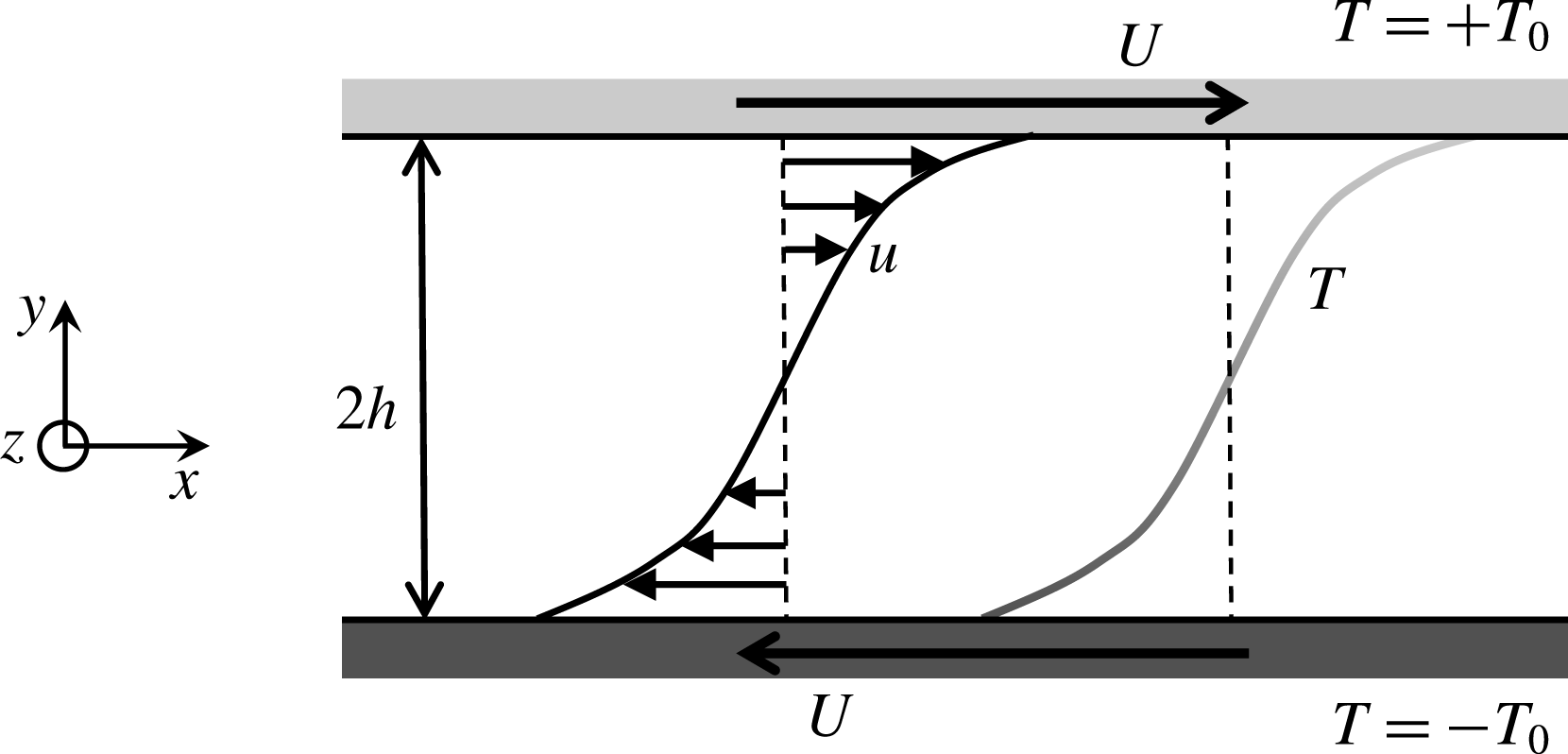
Figure 1 shows the configuration of the velocity and temperature fields. The flow is driven by the two parallel plates moving in the opposite directions at a constant speed
 $U$
. The upper (or lower) wall surface is held at higher (or lower) constant temperature
 $+T_{0}$
(or
 $-T_{0}$
). The coordinates,
 $x$
,
 $y$
and
 $z$
(or
 $x_{1}$
,
 $x_{2}$
and
 $x_{3}$
), are used for the representation of the streamwise, the wall-normal and the spanwise directions, respectively, and their origin is on the midplane of the two plates separated by a distance
 $2h$
. The corresponding components of the velocity
 $\boldsymbol{u}(x,y,z)$
are given by
 $u$
,
 $v$
and
 $w$
(or
 $u_{1}$
,
 $u_{2}$
and
 $u_{3}$
) in the streamwise, the wall-normal and the spanwise directions, respectively.
Let us consider heat transfer in an incompressible time-independent velocity field fulfilling the continuity equation
 $$\begin{eqnarray}\frac{\unicode[STIX]{x2202}u_{i}}{\unicode[STIX]{x2202}x_{i}}=0.\end{eqnarray}$$
Here a question arises: which leads to optimal heat transfer enhancement, a time-independent velocity field or a time-dependent velocity field (see Souza & Doering (Reference Souza and Doering2015a
,Reference Souza and Doering
b
) for the time-dependent version of optimisation problems). In this study, we consider a time-independent velocity field since it is simpler and so much preferable as a target state for flow control. We suppose that the temperature field
 $T(x,y,z)$
is determined as a solution to an advection-diffusion equation
 $$\begin{eqnarray}\frac{\unicode[STIX]{x2202}}{\unicode[STIX]{x2202}x_{j}}(u_{j}T)=\unicode[STIX]{x1D705}\frac{\unicode[STIX]{x2202}^{2}T}{\unicode[STIX]{x2202}x_{j}^{2}},\end{eqnarray}$$
where
 $\unicode[STIX]{x1D705}$
denotes thermal diffusivity. The velocity and temperature fields are supposed to be periodic in the
 $x$
- and
 $z$
-directions with the periods,
 $L_{x}$
and
 $L_{z}$
. The boundary conditions
 $$\begin{eqnarray}u(\,y=\pm h)=\pm U,\quad v(y=\pm h)=w(y=\pm h)=0;\quad T(y=\pm h)=\pm T_{0}\end{eqnarray}$$
are imposed on the walls.
2.2 Scalar dissipation and heat flux
We introduce the
 $xz$
-average and the
 $xyz$
-average given respectively by
 $$\begin{eqnarray}\displaystyle & \displaystyle \langle \cdot \rangle _{xz}=\frac{1}{L_{x}L_{z}}\int _{0}^{L_{x}}\int _{0}^{L_{z}}\cdot \,\text{d}x\,\text{d}z, & \displaystyle\end{eqnarray}$$
 $$\begin{eqnarray}\displaystyle & \displaystyle \langle \cdot \rangle _{xyz}=\frac{1}{2hL_{x}L_{z}}\int _{0}^{L_{x}}\int _{-h}^{h}\int _{0}^{L_{z}}\cdot \,\text{d}x\,\text{d}y\,\text{d}z. & \displaystyle\end{eqnarray}$$
We take the
 $xz$
-average of (2.2) to obtain
 $$\begin{eqnarray}\displaystyle \frac{\text{d}}{\text{d}y}\langle vT\rangle _{xz}=\unicode[STIX]{x1D705}\frac{\text{d}^{2}}{\text{d}y^{2}}\langle T\rangle _{xz}, & & \displaystyle\end{eqnarray}$$
the
 $y$
-integration of which gives us the total heat flux
 $$\begin{eqnarray}\displaystyle \langle vT\rangle _{xz}-\unicode[STIX]{x1D705}\frac{\text{d}}{\text{d}y}\langle T\rangle _{xz}=-\unicode[STIX]{x1D705}\frac{\text{d}}{\text{d}y}\langle T\rangle _{xz}(y=-h)=\text{const}. & & \displaystyle\end{eqnarray}$$
at any wall-normal position
 $y$
. By further taking the average of (2.7) in the
 $y$
-direction we have
 $$\begin{eqnarray}\displaystyle \langle vT\rangle _{xyz}-\unicode[STIX]{x1D705}\frac{T_{0}}{h}=-\unicode[STIX]{x1D705}\frac{\text{d}}{\text{d}y}\langle T\rangle _{xz}(y=-h). & & \displaystyle\end{eqnarray}$$
Now we decompose the temperature into a conductive state and a fluctuation about it as
 $$\begin{eqnarray}\displaystyle T=T_{0}\frac{y}{h}+\unicode[STIX]{x1D703}. & & \displaystyle\end{eqnarray}$$
The boundary conditions of the temperature fluctuation
 $\unicode[STIX]{x1D703}$
are
 $$\begin{eqnarray}\displaystyle \unicode[STIX]{x1D703}(y=\pm h)=0. & & \displaystyle\end{eqnarray}$$
The substitution of decomposition (2.9) in (2.8) yields
 $$\begin{eqnarray}\displaystyle \langle v\unicode[STIX]{x1D703}\rangle _{xyz}=-\unicode[STIX]{x1D705}\frac{\text{d}}{\text{d}y}\langle \unicode[STIX]{x1D703}\rangle _{xz}(y=-h). & & \displaystyle\end{eqnarray}$$
We substitute decomposition (2.9) for (2.2) to have
 $$\begin{eqnarray}\displaystyle \frac{\unicode[STIX]{x2202}}{\unicode[STIX]{x2202}x_{j}}(u_{j}\unicode[STIX]{x1D703})+v\frac{T_{0}}{h}=\unicode[STIX]{x1D705}\frac{\unicode[STIX]{x2202}^{2}\unicode[STIX]{x1D703}}{\unicode[STIX]{x2202}x_{j}^{2}}. & & \displaystyle\end{eqnarray}$$
The product of (2.12) with
 $\unicode[STIX]{x1D703}$
gives us
 $$\begin{eqnarray}\displaystyle \frac{\unicode[STIX]{x2202}}{\unicode[STIX]{x2202}x_{j}}\left(u_{j}\frac{1}{2}\unicode[STIX]{x1D703}^{2}\right)+v\unicode[STIX]{x1D703}\frac{T_{0}}{h}=\unicode[STIX]{x1D705}\frac{\unicode[STIX]{x2202}}{\unicode[STIX]{x2202}x_{j}}\left(\unicode[STIX]{x1D703}\frac{\unicode[STIX]{x2202}\unicode[STIX]{x1D703}}{\unicode[STIX]{x2202}x_{j}}\right)-\unicode[STIX]{x1D705}\left(\frac{\unicode[STIX]{x2202}\unicode[STIX]{x1D703}}{\unicode[STIX]{x2202}x_{j}}\right)^{2}. & & \displaystyle\end{eqnarray}$$
By further taking the
 $xyz$
-average of (2.13) and taking into account boundary conditions (2.10), we obtain
 $$\begin{eqnarray}\displaystyle \frac{T_{0}}{h}\langle v\unicode[STIX]{x1D703}\rangle _{xyz}=-\unicode[STIX]{x1D705}\langle |\unicode[STIX]{x1D735}\unicode[STIX]{x1D703}|^{2}\rangle _{xyz}, & & \displaystyle\end{eqnarray}$$
where the right-hand side represents the dissipation of variance
 $\unicode[STIX]{x1D703}^{2}$
, hereafter referred to as ‘scalar dissipation’. As a consequence, we have the expression of the wall heat flux
 $$\begin{eqnarray}\displaystyle -\unicode[STIX]{x1D705}\frac{\text{d}}{\text{d}y}\langle T\rangle _{xz}(y=+h)=-\unicode[STIX]{x1D705}\frac{\text{d}}{\text{d}y}\langle T\rangle _{xz}(y=-h)=-\frac{\unicode[STIX]{x1D705}h}{T_{0}}\langle |\unicode[STIX]{x1D735}\unicode[STIX]{x1D703}|^{2}\rangle _{xyz}-\unicode[STIX]{x1D705}\frac{T_{0}}{h}. & & \displaystyle\end{eqnarray}$$
2.3 Energy dissipation and momentum flux
The steady motion of a viscous fluid is described by the Navier–Stokes equation
 $$\begin{eqnarray}\displaystyle \frac{\unicode[STIX]{x2202}}{\unicode[STIX]{x2202}x_{j}}(u_{i}u_{j})=-\frac{1}{\unicode[STIX]{x1D70C}}\frac{\unicode[STIX]{x2202}p}{\unicode[STIX]{x2202}x_{i}}+\unicode[STIX]{x1D708}\frac{\unicode[STIX]{x2202}^{2}u_{i}}{\unicode[STIX]{x2202}x_{j}^{2}}+f_{i}, & & \displaystyle\end{eqnarray}$$
where
 $p$
,
 $\unicode[STIX]{x1D70C}$
,
 $\unicode[STIX]{x1D708}$
and
 $f_{i}$
are pressure, mass density, kinematic viscosity and the
 $i$
th component of external body force per unit mass, respectively. The inner product of (2.16) with the velocity yields the local energy budget equation
 $$\begin{eqnarray}\displaystyle \frac{\unicode[STIX]{x2202}}{\unicode[STIX]{x2202}x_{j}}\left(u_{j}\frac{1}{2}|\boldsymbol{u}|^{2}\right)=-\frac{1}{\unicode[STIX]{x1D70C}}\frac{\unicode[STIX]{x2202}}{\unicode[STIX]{x2202}x_{i}}(pu_{i})+\unicode[STIX]{x1D708}\frac{\unicode[STIX]{x2202}}{\unicode[STIX]{x2202}x_{j}}\left(u_{i}\frac{\unicode[STIX]{x2202}u_{i}}{\unicode[STIX]{x2202}x_{j}}\right)-\unicode[STIX]{x1D708}\left(\frac{\unicode[STIX]{x2202}u_{i}}{\unicode[STIX]{x2202}x_{j}}\right)^{2}+u_{i}\,f_{i}. & & \displaystyle\end{eqnarray}$$
By taking the
 $xyz$
-average of (2.17) and taking into account boundary conditions (2.3), we obtain the total energy budget equation
 $$\begin{eqnarray}\displaystyle \frac{\unicode[STIX]{x1D708}}{2}\left[\frac{\text{d}}{\text{d}y}\langle u\rangle _{xz}(y=+h)+\frac{\text{d}}{\text{d}y}\langle u\rangle _{xz}(y=-h)\right]=\frac{\unicode[STIX]{x1D708}h}{U}\langle |\unicode[STIX]{x1D735}\boldsymbol{u}|^{2}\rangle _{xyz}-\frac{h}{U}\langle u_{i}\,f_{i}\rangle _{xyz}, & & \displaystyle\end{eqnarray}$$
where we have supposed a null mean pressure gradient in the wall-parallel (
 $x$
- and
 $z$
-) directions. The left-hand side of (2.18) is mean wall shear stress, while the first and second terms in the right-hand side originate from energy dissipation and an energy input by the external force, respectively.
2.4 Objective functional and Euler–Lagrange equation
Let us now consider the optimisation problem of a functional to find an optimal state for the dissimilarity between momentum and heat transfer. As can be seen from (2.15) and (2.18), the wall heat flux corresponds to the total scalar dissipation, and the wall momentum flux (i.e. the skin friction) is related with the total energy dissipation. Therefore, we shall search for an optimal state which maximises the functional
 $J\{\unicode[STIX]{x1D703},\boldsymbol{u},p^{\ast },\unicode[STIX]{x1D703}^{\ast }\}$
given by
 $$\begin{eqnarray}\displaystyle J & = & \displaystyle \frac{1}{2}\unicode[STIX]{x1D716}\frac{c_{p}\unicode[STIX]{x1D705}}{T_{0}}\langle |\unicode[STIX]{x1D735}\unicode[STIX]{x1D703}|^{2}\rangle _{xyz}-\frac{1}{2}\unicode[STIX]{x1D708}\langle |\unicode[STIX]{x1D735}\boldsymbol{u}|^{2}\rangle _{xyz}\nonumber\\ \displaystyle & & \displaystyle +\,\frac{1}{\unicode[STIX]{x1D70C}}\left\langle p^{\ast }\frac{\unicode[STIX]{x2202}u_{i}}{\unicode[STIX]{x2202}x_{i}}\right\rangle _{xyz}+\unicode[STIX]{x1D716}\frac{c_{p}}{T_{0}}\left\langle \unicode[STIX]{x1D703}^{\ast }\left(u_{j}\frac{\unicode[STIX]{x2202}\unicode[STIX]{x1D703}}{\unicode[STIX]{x2202}x_{j}}+v\frac{T_{0}}{h}-\unicode[STIX]{x1D705}\frac{\unicode[STIX]{x2202}^{2}\unicode[STIX]{x1D703}}{\unicode[STIX]{x2202}x_{j}^{2}}\right)\right\rangle _{xyz},\end{eqnarray}$$
where
 $\unicode[STIX]{x1D716}$
(
 ${>}0$
) is the dimensionless weight of the contribution from the heat transfer against the momentum transfer,
 $c_{p}$
is specific heat at constant pressure and
 $p^{\ast }(x,y,z)$
and
 $\unicode[STIX]{x1D703}^{\ast }(x,y,z)$
represent Lagrangian multipliers. We suppose that
 $\unicode[STIX]{x1D703}^{\ast }$
satisfies boundary conditions on the walls,
 $$\begin{eqnarray}\displaystyle \unicode[STIX]{x1D703}^{\ast }(y=\pm 1)=0. & & \displaystyle\end{eqnarray}$$
By introducing the following dimensionless quantities
 $$\begin{eqnarray}x_{i}^{\prime }=\frac{x_{i}}{h},\quad J^{\prime }=\frac{J}{U^{3}/h},\quad \unicode[STIX]{x1D703}^{\prime }=\frac{\unicode[STIX]{x1D703}}{T_{0}},\quad u_{i}^{\prime }=\frac{u_{i}}{U},\quad {p^{\ast }}^{\prime }=\frac{p^{\ast }}{\unicode[STIX]{x1D70C}U^{2}},\quad {\unicode[STIX]{x1D703}^{\ast }}^{\prime }=\frac{\unicode[STIX]{x1D703}^{\ast }}{T_{0}},\end{eqnarray}$$
we rewrite the objective functional (2.19) in a dimensionless form as
 $$\begin{eqnarray}\displaystyle J & = & \displaystyle \frac{1}{2}\unicode[STIX]{x1D706}\frac{1}{Re\,Pr}\langle |\unicode[STIX]{x1D735}\unicode[STIX]{x1D703}|^{2}\rangle _{xyz}-\frac{1}{2}\frac{1}{Re}\langle |\unicode[STIX]{x1D735}\boldsymbol{u}|^{2}\rangle _{xyz}+\left\langle p^{\ast }\frac{\unicode[STIX]{x2202}u_{j}}{\unicode[STIX]{x2202}x_{j}}\right\rangle _{xyz}\nonumber\\ \displaystyle & & \displaystyle +\unicode[STIX]{x1D706}\left\langle \unicode[STIX]{x1D703}^{\ast }\left(u_{j}\frac{\unicode[STIX]{x2202}\unicode[STIX]{x1D703}}{\unicode[STIX]{x2202}x_{j}}+v-\frac{1}{Re\,Pr}\frac{\unicode[STIX]{x2202}^{2}\unicode[STIX]{x1D703}}{\unicode[STIX]{x2202}x_{j}^{2}}\right)\right\rangle _{xyz},\end{eqnarray}$$
where we have dropped the primes attached to the dimensionless quantities,
 $$\begin{eqnarray}\displaystyle \unicode[STIX]{x1D706}=\frac{\unicode[STIX]{x1D716}}{Ec} & & \displaystyle\end{eqnarray}$$
is new dimensionless weight, and
 $$\begin{eqnarray}\displaystyle Re=\frac{Uh}{\unicode[STIX]{x1D708}},\quad Pr=\frac{\unicode[STIX]{x1D708}}{\unicode[STIX]{x1D705}},\quad Ec=\frac{U^{2}}{c_{p}T_{0}} & & \displaystyle\end{eqnarray}$$
are the Reynolds number, the Prandtl number and the Eckert number, respectively. Usually
 $Ec\ll 1$
, and thus we suppose that
 $\unicode[STIX]{x1D716}\ll 1$
so that we may take
 $\unicode[STIX]{x1D706}\sim 10^{0}$
. We decompose
 $\boldsymbol{u},\unicode[STIX]{x1D703},p^{\ast }$
and
 $\unicode[STIX]{x1D703}^{\ast }$
into references and infinitesimal perturbations as
 $$\begin{eqnarray}\displaystyle \unicode[STIX]{x1D703}=\overline{\unicode[STIX]{x1D703}}+\unicode[STIX]{x1D6FF}\unicode[STIX]{x1D703},\quad \boldsymbol{u}=\overline{\boldsymbol{u}}+\unicode[STIX]{x1D6FF}\boldsymbol{u},\quad p^{\ast }=\overline{p^{\ast }}+\unicode[STIX]{x1D6FF}p^{\ast },\quad \unicode[STIX]{x1D703}^{\ast }=\overline{\unicode[STIX]{x1D703}^{\ast }}+\unicode[STIX]{x1D6FF}\unicode[STIX]{x1D703}^{\ast }. & & \displaystyle\end{eqnarray}$$
Substituting (2.25) into (2.22), using integration by parts and recalling boundary conditions (2.3), (2.10) and (2.20), we obtain the first variation of
 $J$
as
 $$\begin{eqnarray}\displaystyle \unicode[STIX]{x1D6FF}J & = & \displaystyle \left\langle \left(-\frac{\unicode[STIX]{x2202}\overline{p^{\ast }}}{\unicode[STIX]{x2202}x_{i}}+\frac{1}{Re}\frac{\unicode[STIX]{x2202}^{2}\overline{u_{i}}}{\unicode[STIX]{x2202}x_{j}^{2}}+\unicode[STIX]{x1D706}\overline{\unicode[STIX]{x1D703}^{\ast }}\frac{\unicode[STIX]{x2202}\overline{\unicode[STIX]{x1D703}}}{\unicode[STIX]{x2202}x_{i}}+\unicode[STIX]{x1D706}\overline{\unicode[STIX]{x1D703}^{\ast }}\unicode[STIX]{x1D6FF}_{i2}\right)\unicode[STIX]{x1D6FF}u_{i}\right\rangle _{xyz}\nonumber\\ \displaystyle & & \displaystyle -\,\left\langle \unicode[STIX]{x1D706}\left(\overline{u_{j}}\frac{\unicode[STIX]{x2202}\overline{\unicode[STIX]{x1D703}^{\ast }}}{\unicode[STIX]{x2202}x_{j}}+\frac{1}{Re\,Pr}\frac{\unicode[STIX]{x2202}^{2}\overline{\unicode[STIX]{x1D703}^{\ast }}}{\unicode[STIX]{x2202}x_{j}^{2}}+\frac{1}{Re\,Pr}\frac{\unicode[STIX]{x2202}^{2}\overline{\unicode[STIX]{x1D703}}}{\unicode[STIX]{x2202}x_{j}^{2}}\right)\unicode[STIX]{x1D6FF}\unicode[STIX]{x1D703}\right\rangle _{xyz}\nonumber\\ \displaystyle & & \displaystyle +\,\left\langle \unicode[STIX]{x1D706}\left(\overline{u_{j}}\frac{\unicode[STIX]{x2202}\overline{\unicode[STIX]{x1D703}}}{\unicode[STIX]{x2202}x_{j}}+\overline{v}-\frac{1}{Re\,Pr}\frac{\unicode[STIX]{x2202}^{2}\overline{\unicode[STIX]{x1D703}}}{\unicode[STIX]{x2202}x_{j}^{2}}\right)\unicode[STIX]{x1D6FF}\unicode[STIX]{x1D703}^{\ast }\right\rangle _{xyz}+\left\langle \left(\frac{\unicode[STIX]{x2202}\overline{u_{i}}}{\unicode[STIX]{x2202}x_{i}}\right)\unicode[STIX]{x1D6FF}p^{\ast }\right\rangle _{xyz}.\end{eqnarray}$$
A stationary point, at which the first variation of
 $J$
vanishes, i.e.
 $\unicode[STIX]{x1D6FF}J=0$
, for any perturbation
 $\unicode[STIX]{x1D6FF}\boldsymbol{u},\unicode[STIX]{x1D6FF}\unicode[STIX]{x1D703},\unicode[STIX]{x1D6FF}\unicode[STIX]{x1D703}^{\ast }$
and
 $\unicode[STIX]{x1D6FF}p^{\ast }$
, is determined by the Euler–Lagrange equations
 $$\begin{eqnarray}\displaystyle & \displaystyle \frac{\unicode[STIX]{x1D6FF}J}{\unicode[STIX]{x1D6FF}u_{i}}\equiv -\frac{\unicode[STIX]{x2202}p^{\ast }}{\unicode[STIX]{x2202}x_{i}}+\frac{1}{Re}\frac{\unicode[STIX]{x2202}^{2}u_{i}}{\unicode[STIX]{x2202}x_{j}^{2}}+\unicode[STIX]{x1D706}\unicode[STIX]{x1D703}^{\ast }\frac{\unicode[STIX]{x2202}\unicode[STIX]{x1D703}}{\unicode[STIX]{x2202}x_{i}}+\unicode[STIX]{x1D706}\unicode[STIX]{x1D703}^{\ast }\unicode[STIX]{x1D6FF}_{i2}=0, & \displaystyle\end{eqnarray}$$
 $$\begin{eqnarray}\displaystyle & \displaystyle \frac{\unicode[STIX]{x1D6FF}J}{\unicode[STIX]{x1D6FF}\unicode[STIX]{x1D703}}\equiv u_{j}\frac{\unicode[STIX]{x2202}\unicode[STIX]{x1D703}^{\ast }}{\unicode[STIX]{x2202}x_{j}}+\frac{1}{Re\,Pr}\frac{\unicode[STIX]{x2202}^{2}\unicode[STIX]{x1D703}^{\ast }}{\unicode[STIX]{x2202}x_{j}^{2}}+\frac{1}{Re\,Pr}\frac{\unicode[STIX]{x2202}^{2}\unicode[STIX]{x1D703}}{\unicode[STIX]{x2202}x_{j}^{2}}=0, & \displaystyle\end{eqnarray}$$
 $$\begin{eqnarray}\displaystyle & \displaystyle \frac{\unicode[STIX]{x1D6FF}J}{\unicode[STIX]{x1D6FF}\unicode[STIX]{x1D703}^{\ast }}\equiv u_{j}\frac{\unicode[STIX]{x2202}\unicode[STIX]{x1D703}}{\unicode[STIX]{x2202}x_{j}}+v-\frac{1}{Re\,Pr}\frac{\unicode[STIX]{x2202}^{2}\unicode[STIX]{x1D703}}{\unicode[STIX]{x2202}x_{j}^{2}}=0, & \displaystyle\end{eqnarray}$$
 $$\begin{eqnarray}\displaystyle & \displaystyle \frac{\unicode[STIX]{x1D6FF}J}{\unicode[STIX]{x1D6FF}p^{\ast }}\equiv \frac{\unicode[STIX]{x2202}u_{i}}{\unicode[STIX]{x2202}x_{i}}=0. & \displaystyle\end{eqnarray}$$
For the streamwise-independent case (
 $\unicode[STIX]{x2202}/\unicode[STIX]{x2202}x(\cdot )=0$
), the streamwise velocity can be decoupled from the other velocity components, since the streamwise velocity
 $u$
is uniquely determined by the
 $x$
-component of (2.27) as
 $u(\boldsymbol{x})=y$
. The optimisation problem for this case can be shown to correspond to the two-dimensional free-slip variational problem recently formulated by Hassanzadeh et al. (Reference Hassanzadeh, Chini and Doering2014) for fixed enstrophy constraint. More recently, Hassanzadeh et al.’s configuration has been extended by Souza (Reference Souza2016) to the two-dimensional boundary-value problem of no-slip walls at rest. We have confirmed that the scaling property of our decoupled two-dimensional optimal states to be shown in figure 16 is consistent with that in Souza (Reference Souza2016).
3 Numerical procedures
3.1 Finding optimal states
We find velocity fields which give a maximal value of the objective functional
 $J$
with a combination of the steepest ascent method and the Newton–Krylov method. To globally seek a maximal point of
 $J$
, we start with finding initial guesses in the following procedure.
- Step. 1
-
Start from an arbitrary velocity field
 $\boldsymbol{u}$
which satisfies the continuity equation (2.1) and boundary condition (2.3).
- Step. 2
-
For given
$\boldsymbol{u}$
, solve (2.29) to obtain
$\unicode[STIX]{x1D703}$
. - Step. 3
-
For given
$\boldsymbol{u}$
and obtained
$\unicode[STIX]{x1D703}$
from Step. 2, solve (2.28) to find
$\unicode[STIX]{x1D703}^{\ast }$
. - Step. 4
-
Since
$\boldsymbol{u}$
,
$\unicode[STIX]{x1D703}$
and
$\unicode[STIX]{x1D703}^{\ast }$
respectively satisfy the Euler–Lagrange equations (2.28)–(2.30), the first variation
$\unicode[STIX]{x1D6FF}J$
can be expressed, in terms of the only functional derivative
$\widehat{u_{i}}\equiv \unicode[STIX]{x1D6FF}J/\unicode[STIX]{x1D6FF}u_{i}$
, as (3.1)
$$\begin{eqnarray}\unicode[STIX]{x1D6FF}J=\langle \widehat{u_{i}}\unicode[STIX]{x1D6FF}u_{i}\rangle _{xyz}.\end{eqnarray}$$
Using the functional derivative
$\widehat{\boldsymbol{u}}$
, renew the velocity field as (3.2)
$$\begin{eqnarray}\boldsymbol{u}^{new}=\boldsymbol{u}+s\widehat{\boldsymbol{u}},\end{eqnarray}$$
where
$s$
is a small positive constant to be taken as
$s\sim 10^{-2}$
. - Step. 5
-
Repeat Step. 2–Step. 4.


By employing the obtained initial guesses, we perform the Newton–Krylov iteration to obtain nonlinear solutions to the Euler–Lagrange equations (2.27)–(2.30). The details of the spatial discretisation and the Newton–Krylov iteration are described in appendix A.
3.2 Direct numerical simulation of turbulent plane Couette flow
For comparison with optimal states obtained by the maximisation of the functional
 $J$
, direct numerical simulations are also performed for turbulent momentum and heat transfer in plane Couette flow. In the simulations we numerically integrate the incompressible Navier–Stokes equation and the advection-diffusion equation for temperature supplemented by boundary conditions (2.3). The temperature is treated as a passive scalar with no buoyancy effect. The evolution equations are discretised employing a spectral Galerkin method based on the expansions (A 10) and (A 13). Time marching of the equations is done with a combination of the Crank–Nicholson and second-order Adams–Bashforth scheme. The Prandtl number
 $Pr$
is set to unity. Turbulence data are accumulated in the range of the Reynolds number,
 $Re=500$
–
 $10\,000$
, in a computational domain of
 $(L_{x},L_{y},L_{z})=(2\unicode[STIX]{x03C0},2,\unicode[STIX]{x03C0})$
.
3.3 Global convergence and dependence on domain size and weight
$\unicode[STIX]{x1D706}$

Objective functional
 $J$
against the number of the iteration described in § 3.1 for various initial guesses at
 $Re=100$
for
 $Pr=1$
and
 $\unicode[STIX]{x1D706}=1$
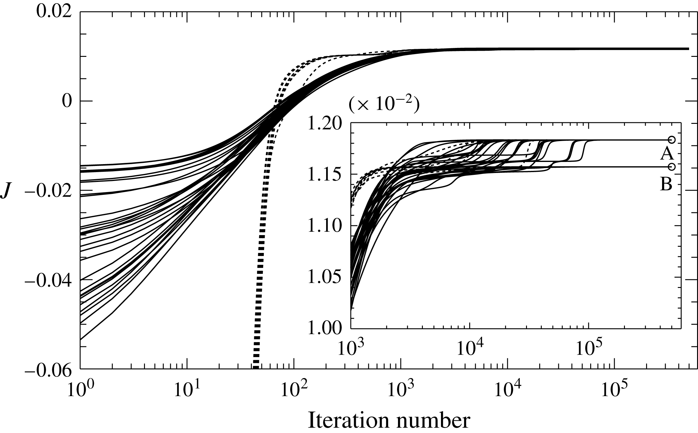
. Forty initial guesses (10 each) are taken from turbulent flow fields at
 $Re=1000$
, 2000 and 3000 (solid curves) and random flow fields (dashed curves). Twenty nine of them converge to a local maximum A, and the others tend to a local maximum B.

Two local maxima of objective functional
 $J$
at
 $Re=100$
for
 $Pr=1$
and
 $\unicode[STIX]{x1D706}=1$
.

We perform the maximisation of the functional
 $J$
starting with 40 different initial guesses extracted from turbulent and random flow fields in order to examine the dependence of a computed local maximum on the initial guesses. Figure 2 shows the functional
 $J$
against the number of the iteration mentioned in § 3.1 for the distinct 40 initial guesses at
 $Re=100$
for
 $Pr=1$
and
 $\unicode[STIX]{x1D706}=1$
. For all the initial guesses, the value of
 $J$
rapidly approaches the vicinity of the two local maxima to be mentioned just below. We have eventually obtained the two different local maxima (the larger local maximum is labelled as A, and the smaller one as B). Table 1 compares the values of
 $J$
together with the total scalar dissipation
 $\unicode[STIX]{x1D700}_{S}$
and the total energy dissipation
 $\unicode[STIX]{x1D700}_{E}$
,
 $$\begin{eqnarray}\displaystyle \unicode[STIX]{x1D700}_{S}=\frac{1}{Re\,Pr}\langle |\unicode[STIX]{x1D735}T|^{2}\rangle _{xyz},\quad \unicode[STIX]{x1D700}_{E}=\frac{1}{Re}\langle |\unicode[STIX]{x1D735}\boldsymbol{u}|^{2}\rangle _{xyz}, & & \displaystyle\end{eqnarray}$$
between the local maxima A and B.
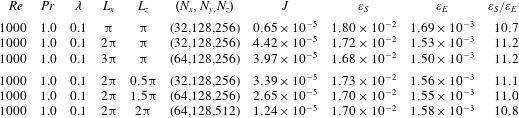
Dependence on computational domain size.
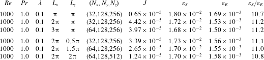
The optimal velocity fields exhibit three-dimensional structures which consist of large-scale streamwise circulation rolls and smaller-scale quasi-streamwise vortex tubes near the wall (see figures 4 and 5). The size of the large rolls corresponds to half the spanwise period
 $L_{z}/2$
. Table 2 summarises each maximal state obtained in the various domains at
 $Re=1000$
for
 $Pr=1$
and
 $\unicode[STIX]{x1D706}=0.1$
. It is found that
 $J$
takes the largest value for
 $(L_{x},L_{z})=(2\unicode[STIX]{x03C0},\unicode[STIX]{x03C0})$
among
 $(L_{x},L_{z})=(\unicode[STIX]{x03C0},\unicode[STIX]{x03C0})$
,
 $(2\unicode[STIX]{x03C0},\unicode[STIX]{x03C0})$
,
 $(3\unicode[STIX]{x03C0},\unicode[STIX]{x03C0})$
;
 $(2\unicode[STIX]{x03C0},0.5\unicode[STIX]{x03C0})$
,
 $(2\unicode[STIX]{x03C0},\unicode[STIX]{x03C0})$
,
 $(2\unicode[STIX]{x03C0},1.5\unicode[STIX]{x03C0})$
,
 $(2\unicode[STIX]{x03C0},2\unicode[STIX]{x03C0})$
, suggesting that there exist finite values of the streamwise and spanwise periods which lead to the global optimal. However, our goal in this paper is not to identify the optimal domain for all the parameters including
 $Re$
. As will be described below, the velocity fields, which are realised as a solution to the Euler–Lagrange equations (2.27)–(2.30), have extremely high performance for heat transfer and exhibit qualitatively similar flow structures being roughly independent of
 $(L_{x},L_{z})$
. The effects of the domain size on the scalar dissipation and the energy dissipation can be seen to be minor.
The optimal states also depend on the weight
 $\unicode[STIX]{x1D706}$
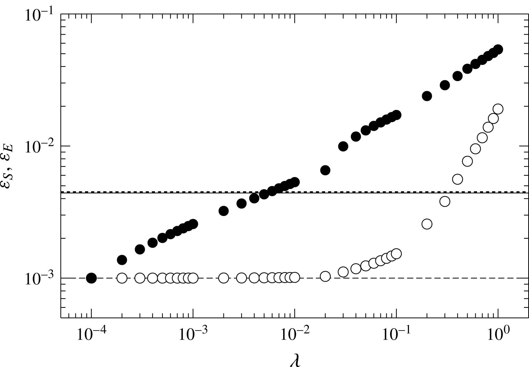
. The dependence is shown in appendix B. In the range of
 $0.02<\unicode[STIX]{x1D706}<0.4$
, the optimal states are found to provide higher heat transfer and lower energy dissipation than the turbulent state at
 $Re=1000$
for
 $Pr=1$
. In this range of the weight
 $\unicode[STIX]{x1D706}$
we have confirmed that the optimised velocity fields do not exhibit significantly different flow structures depending on
 $\unicode[STIX]{x1D706}$
.
In the following sections, therefore, we shall present the optimal states in the domain
 $(L_{x},L_{y},L_{z})=(2\unicode[STIX]{x03C0},2,\unicode[STIX]{x03C0})$
for
 $Pr=1$
and
 $\unicode[STIX]{x1D706}=0.1$
. The numerical solutions have been obtained on grid points
 $(N_{x},N_{y},N_{z})=(\text{32,128,256})$
at
 $Re=30{-}900$
and
 $(N_{x},N_{y},N_{z})=(\text{32,256,512})$
at
 $Re=1000{-}10\,000$
.
4 Characteristics of optimal states
4.1 Flow and temperature field
The maximal value of
 $J$
as a function of
 $Re$
for
 $\unicode[STIX]{x1D706}=0.1$
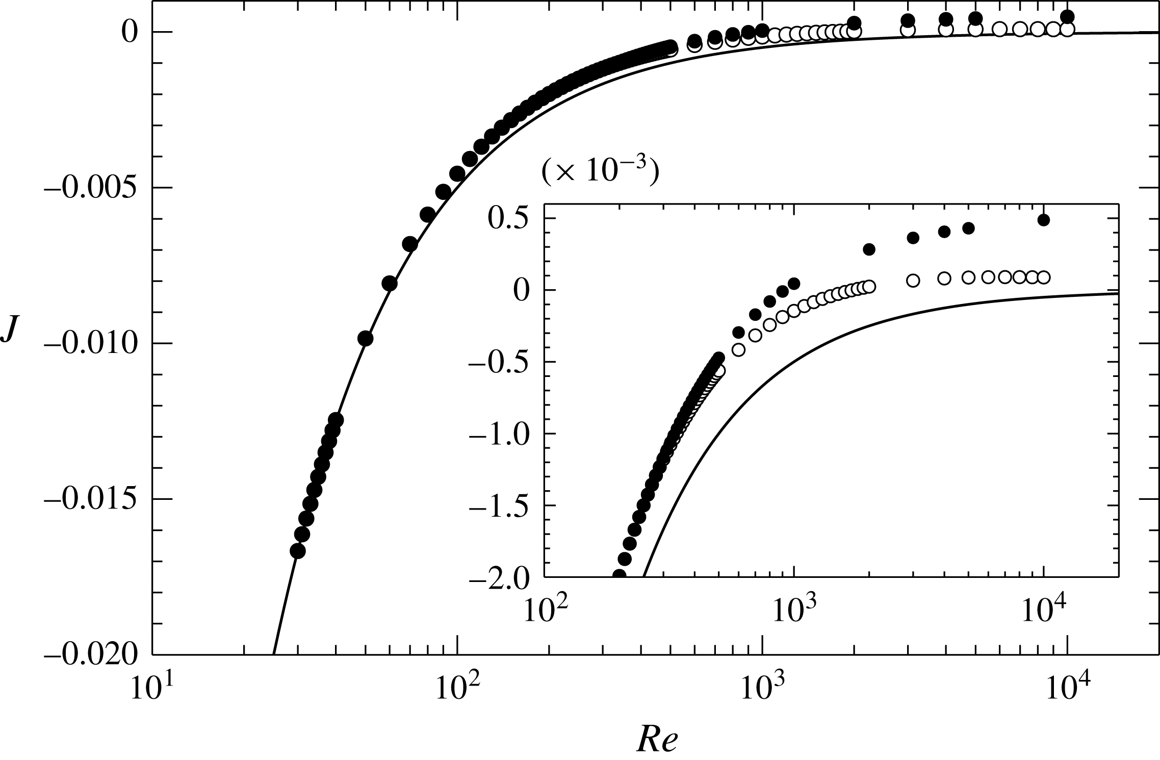
. Filled circles represent the value of
 $J$
for the optimal states, and open circles denote maximised
 $J$
only within a streamwise-independent two-dimensional velocity field. The solid curve represents the value of
 $J$
for the laminar solution,
 $J=-1/(2Re)$
.

Isosurfaces of the streamwise vorticity in the optimal states at (a)
 $Re=50$
, (b)
 $Re=200$
, (c)
 $Re=1000$
and (d)
 $Re=5000$
, for
 $\unicode[STIX]{x1D706}=0.1$
. In (c) and (d), only the isosurfaces in the lower half of the channel (
 $y<0$
) are shown for visualisation of the small-scale vortex structures near the lower wall. Light (or dark) grey objects represent isosurfaces of (a)
 $\unicode[STIX]{x1D714}_{x}=+0.25$
(or
 $-0.25$
), (b)
 $\unicode[STIX]{x1D714}_{x}=+0.25$
(or
 $-0.25$
), (c)
 $\unicode[STIX]{x1D714}_{x}=+0.5$
(or
 $-0.5$
), (d)
 $\unicode[STIX]{x1D714}_{x}=+2$
(or
 $-2$
).

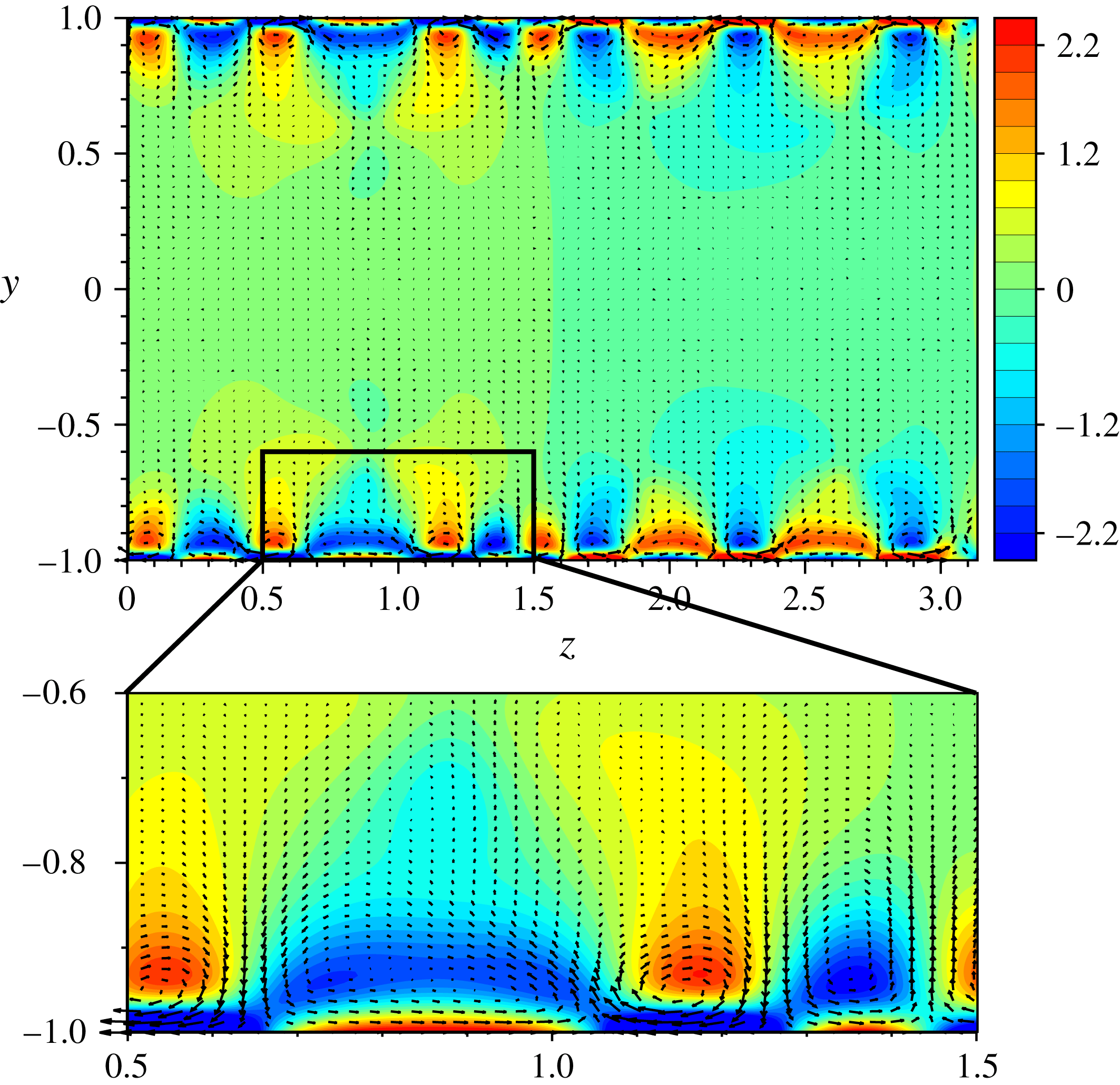
Velocity and temperature fields in the optimal state at (a)
 $Re=50$
, (b)
 $Re=200$
, (c,e)
 $Re=1000$
and (d,f)
 $Re=5000$
, for
 $\unicode[STIX]{x1D706}=0.1$
. (a,b,c,d) The cross-stream velocity vectors (
 $w,v$
) and contours of the temperature field
 $T$
in the plane
 $x=0$
. In (c) and (d), the enlarged views of the near-wall region are also shown. (e,f) The streamwise-averaged cross-stream velocity vectors (
 $\langle w\rangle _{x},\langle v\rangle _{x}$
).

Mean temperature and velocity in the optimal state for
 $\unicode[STIX]{x1D706}=0.1$
.

Figure 3 shows the maximal value of
 $J$
as a function of
 $Re$
for
 $\unicode[STIX]{x1D706}=0.1$
. The maximised
 $J$
only within a streamwise-independent two-dimensional velocity field is also plotted for comparison purposes. The solid curve represents the value of
 $J$
for the laminar solution
 $\boldsymbol{u}=y\boldsymbol{e}_{x}$
, which is the lower bound of
 $J$
. At low values of
 $Re$
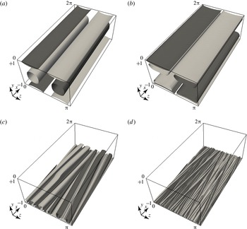
, the optimal state exhibits a streamwise-independent two-dimensional velocity field as seen in figure 4, where the isosurfaces of the positive and negative streamwise vorticity
 $\unicode[STIX]{x1D714}_{x}$
are shown for the optimal states at
 $Re=50$
,
 $200$
,
 $1000$
and
 $5000$
. At the higher Reynolds numbers
 $Re=1000$
and 5000, streamwise-dependent three-dimensional structures, i.e. spanwise-inclined vortex tubes, with stronger
 $\unicode[STIX]{x1D714}_{x}$
appear near the wall. We shall discuss the onset of the spanwise inclination of the structures and its effects on heat transfer in § 6. In figure 4(c,d), only the isosurfaces in the lower half of the channel (
 $y<0$
) are shown for visualisation of the near-wall vortices. At
 $Re=5000$
a large number of smaller vortex structures with much stronger
 $\unicode[STIX]{x1D714}_{x}$
are observed in the close vicinity of the wall. Note that such small-scale intense vortices do not emerge near the wall in the two-dimensional optimal velocity fields (figure 4
a,b). Although the formation of the small-scale structures increases the energy dissipation, it also significantly enhances the scalar dissipation. As a result of these counteractions, the three-dimensional fields could be an optimal state at higher
 $Re$
. Even when the domain size or the weight
 $\unicode[STIX]{x1D706}$
is changed, we have obtained the optimal states which represent qualitatively similar three-dimensional structures.
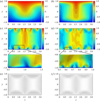
Figure 5(a–d) shows the cross-stream velocity field
 $(w,v)$
and the temperature field
 $T$
in the optimal states at
 $Re=50$
,
 $200$
,
 $1000$
and
 $5000$
. The two-dimensional optimal states at
 $Re=50$
and 200 (figure 5
a,b) consist of the two large-scale circulation rolls which are reminiscent of thermal convection and play a role in heat transfer from the upper wall to the lower wall. Near the walls, the regions with the high temperature gradient are formed by the effects of the circulation rolls, and the gradient gets higher as
 $Re$
increases. Meanwhile, the three-dimensional optimal state at
 $Re=1000$
and 5000 (figure 5
c,d) exhibit a more complicated flow and temperature field. Similar to the two-dimensional states, there are the large-scale circulation rolls with the width of half the spanwise period
 $L_{z}$
(
 $=\unicode[STIX]{x03C0}$
). The wall-normal component of the velocity is dominant in between the circulation rolls. Small-scale vortices are observed only in the near-wall regions. They produce the regions with high temperature gradient by pushing the hotter (or colder) fluid onto the lower (or upper) wall. Figure 5(e,f) shows the streamwise-averaged cross-stream velocity fields at
 $Re=1000$
and
 $5000$
. Even in the averaged fields, the effects of the small-scale vortices can be seen close to the wall at
 $Re=5000$
.
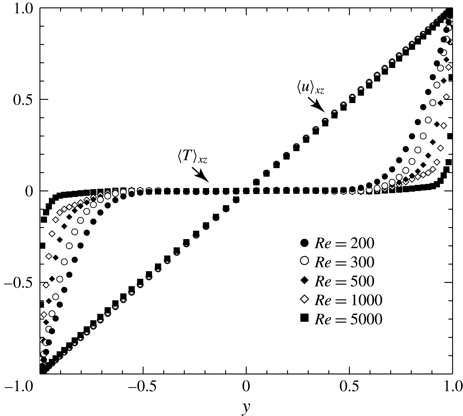
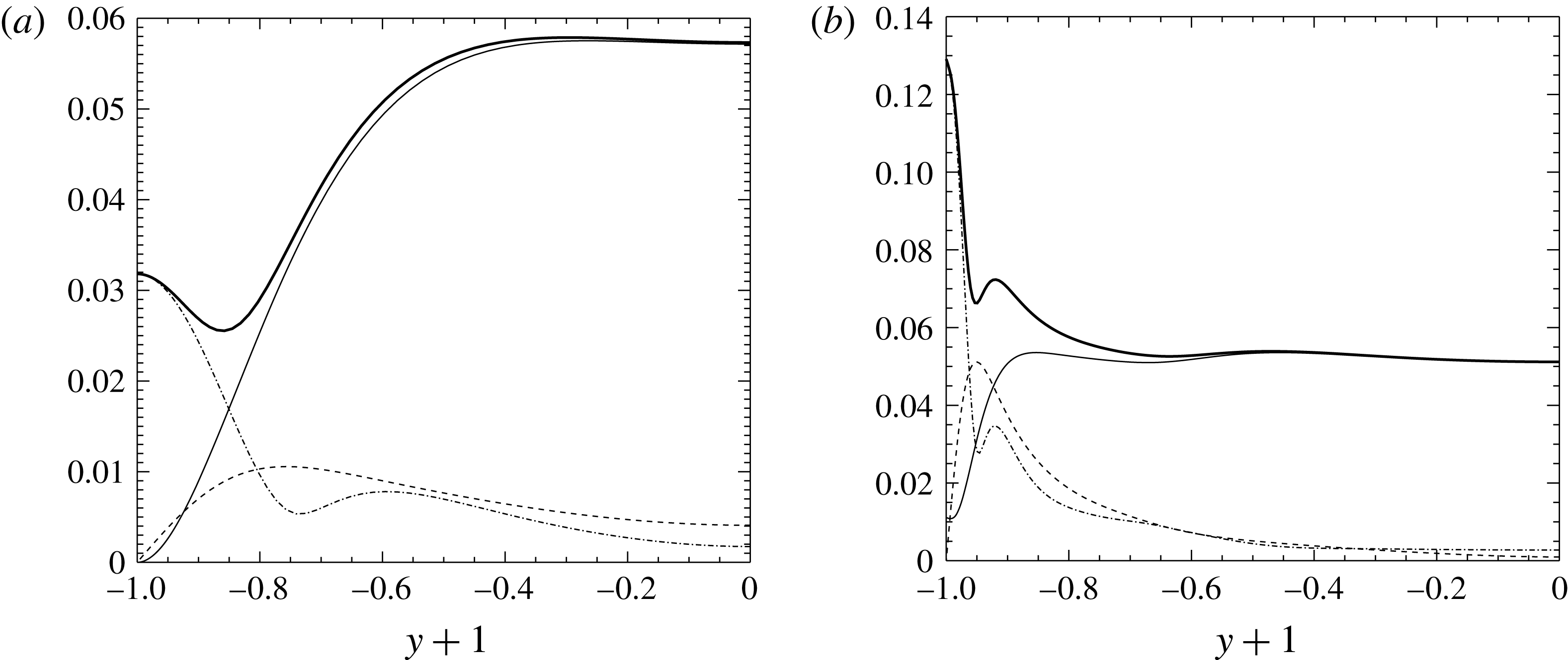
The mean temperature and the mean streamwise velocity profiles of the optimal states are shown in figure 6(a). As
 $Re$
increases, the mean temperature profile is more flattened in the central region of the channel, while the temperature gradient at the walls is higher. On the other hand, the mean velocity profile is almost consistent with a laminar profile. For the streamwise-independent case (i.e.
 $\unicode[STIX]{x2202}(\cdot )/\unicode[STIX]{x2202}x=0$
) seen in the optimal state at
 $Re=200$
, the streamwise velocity
 $u$
is strictly consistent with the laminar profile
 $u=y$
, which is a consequence of the
 $x$
-component of the Euler–Lagrange equation (2.27). At large
 $Re$
, the three-dimensional vortex structure has appeared to bring about the deviation from the laminar profile, shown in figure 6(b), although the deviation is small even at
 $Re=5000$
.
4.2 Wall heat flux and energy dissipation
(a) Stanton number
 $St$
and friction coefficient
 $C_{f}$
as a function of
 $Re$
. The optimal state for
 $\unicode[STIX]{x1D706}=0.1$
: ●,
 $St$
; ○,
 $C_{f}$
. The turbulent flow:
 $\times$
,
 $St$
;
 $+$
,
 $C_{f}$
. The solid line and dashed curve represent
 $C_{f}=2/Re$
for the laminar flow and the empirical formula
 $C_{f}=2(0.2/\log (Re))^{2}$
for the turbulent flow, respectively. (b) Total scalar dissipation
 $\unicode[STIX]{x1D700}_{S}$
, energy dissipation
 $\unicode[STIX]{x1D700}_{E}$
and energy input
 $\langle u_{i}\,f_{i}\rangle _{xyz}$
. The optimal state for
 $\unicode[STIX]{x1D706}=0.1$
: ●,
 $\unicode[STIX]{x1D700}_{S}$
; ○,
 $\unicode[STIX]{x1D700}_{E}$
; ▵,
 $\langle u_{i}\,f_{i}\rangle _{xyz}$
. The turbulent flow:
 $\times$
,
 $\unicode[STIX]{x1D700}_{S}$
;
 $+$
,
 $\unicode[STIX]{x1D700}_{E}$
. The solid line and dashed curve represent
 $1/Re$
and
 $C_{f}/2$
for the laminar flow and the turbulent flow, respectively.

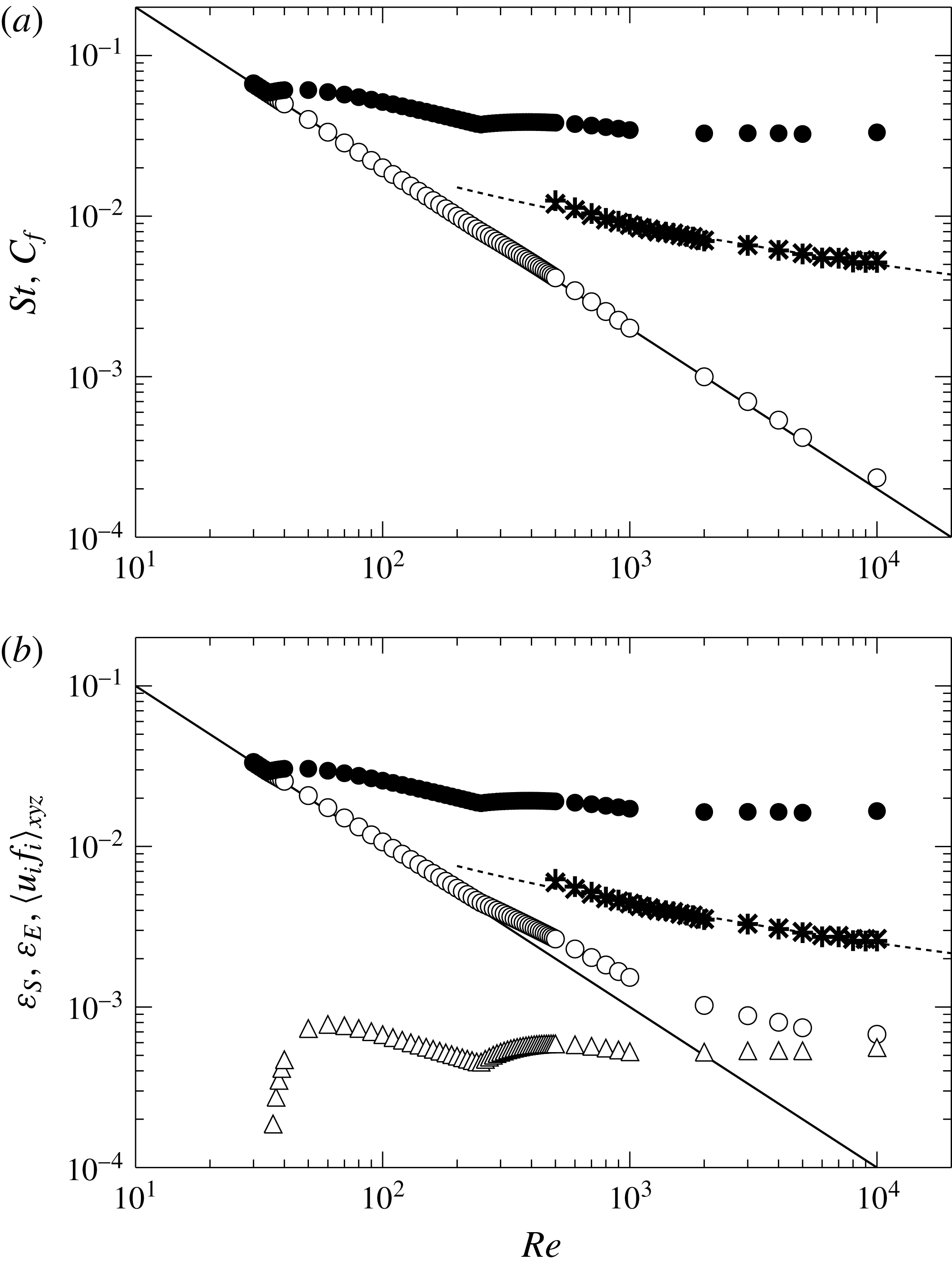
Let us now consider the Stanton number
 $St$
and the friction coefficient
 $C_{f}$
which are respectively defined as
 $$\begin{eqnarray}\displaystyle & \displaystyle St=\frac{1}{Re\,Pr}\left[\frac{\text{d}}{\text{d}y}\langle T\rangle _{xz}(y=+1)+\frac{\text{d}}{\text{d}y}\langle T\rangle _{xz}(y=-1)\right], & \displaystyle\end{eqnarray}$$
 $$\begin{eqnarray}\displaystyle & \displaystyle C_{f}=\frac{1}{Re}\left[\frac{\text{d}}{\text{d}y}\langle u\rangle _{xz}(y=+1)+\frac{\text{d}}{\text{d}y}\langle u\rangle _{xz}(y=-1)\right]. & \displaystyle\end{eqnarray}$$
Note that the similarity between heat and momentum transfer implies that
 $St\approx C_{f}$
for
 $Pr=1$
. Figure 7(a) shows
 $St$
and
 $C_{f}$
in the optimal state for
 $\unicode[STIX]{x1D706}=0.1$
. The solid line and the dashed curve represent the theoretical formula for laminar flow and the empirical formula (Robertson & Johnson Reference Robertson and Johnson1970) for turbulent flow, respectively. The time-averaged
 $St$
and
 $C_{f}$
in turbulent flow are also plotted as a reference. In turbulent flow,
 $St$
and
 $C_{f}$
are almost the same due to the similarity between momentum and heat transfer. In contrast, in the optimal state extremely high
 $St$
is achieved in comparison with turbulence whilst
 $C_{f}$
is comparably low to the laminar flow, decreasing as
 $Re^{-1}$
with increasing
 $Re$
.
The dimensionless versions of budget equations (2.15) and (2.18) are given respectively by
 $$\begin{eqnarray}\displaystyle & \displaystyle \unicode[STIX]{x1D700}_{S}=\frac{1}{2}St, & \displaystyle\end{eqnarray}$$
 $$\begin{eqnarray}\displaystyle & \displaystyle \unicode[STIX]{x1D700}_{E}=\frac{1}{2}C_{f}+\langle u_{i}\,f_{i}\rangle _{xyz}. & \displaystyle\end{eqnarray}$$
The optimal states found in this work require the external force
 $f_{i}$
to satisfy the Navier–Stokes equation, since we have imposed only the divergence-free condition on the velocity field. The external force leads to the additional energy input
 $\langle u_{i}\,f_{i}\rangle _{xyz}$
which has appeared in (4.4). Figure 7(b) shows the total scalar dissipation
 $\unicode[STIX]{x1D700}_{S}$
, the energy dissipation
 $\unicode[STIX]{x1D700}_{E}$
and the energy input
 $\langle u_{i}\,f_{i}\rangle _{xyz}$
. Note that in the case of no external force, the energy budget implies
 $\unicode[STIX]{x1D700}_{E}=C_{f}/2$
. The solid line represents the energy dissipation in the laminar flow, and provides the lower bound of
 $\unicode[STIX]{x1D700}_{E}$
. As
 $Re$
increases,
 $\unicode[STIX]{x1D700}_{E}$
for the optimal state gradually deviates from that of the laminar flow, because of the relatively greater contribution of the energy input
 $\langle u_{i}\,f_{i}\rangle _{xyz}$
. The energy input is positive (or zero for a laminar solution) at any
 $Re$
, but it is quite small in comparison to
 $\unicode[STIX]{x1D700}_{E}$
in the turbulent flow. The significant heat transfer enhancement with small energy dissipation can be confirmed for the optimal state (e.g.
 $\unicode[STIX]{x1D700}_{S}/\unicode[STIX]{x1D700}_{E}\approx 24.6$
at
 $Re=10\,000$
). The spatial distribution of the external force and the local energy input are depicted in appendix C.
5 Hierarchical structure in optimal state
Spectral densities of the wall-normal velocity in the optimal states as a function of the spanwise wavelength
 $l$
for
 $\unicode[STIX]{x1D706}=0.1$
. The distance to the lower wall
 $y+h$
and the wavelength
 $l$
are normalised by (a) the channel half-width
 $h$
and (b) the inner length
 $\unicode[STIX]{x1D6FF}_{T}=T_{0}/(\text{d}\langle T\rangle _{xz}/\text{d}y)(y=-h)$
, respectively. The thick dashed line denotes
 $l=\unicode[STIX]{x03C0}(y+h)$
.

Mean temperature profile (a) and convective heat flux (b) in the optimal states for
 $\unicode[STIX]{x1D706}=0.1$
: ●,
 $Re=1000$
; ○,
 $Re=2000$
; ▪,
 $Re=3000$
; ▫,
 $Re=4000$
; ▴,
 $Re=5000$
. The distance to the wall
 $y+h$
and the temperature
 $T$
are normalised by the inner length and the wall temperature
 $T_{0}$
, respectively. The solid curve and dashed line denote
 $\langle T\rangle _{xz}/T_{0}+1=(y+h)/\unicode[STIX]{x1D6FF}_{T}$
and the logarithmic fit
 $\langle T\rangle _{xz}/T_{0}+1=0.086\ln [(y+h)/\unicode[STIX]{x1D6FF}_{T}]+0.81$
determined in the range
 $1<(y+h)/\unicode[STIX]{x1D6FF}_{T}<10$
, respectively.

Let us discuss the hierarchical structure and its scaling for the optimal state. Just in this section, we restore the dimensional variables, such as
 $\boldsymbol{x},\boldsymbol{u},T$
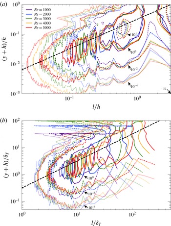
. Figure 8 shows the one-dimensional spectral densities of the wall-normal velocity at
 $Re=1000$
,
 $2000$
,
 $3000$
,
 $4000$
and
 $5000$
. The lateral axis denotes the spanwise wavelength
 $l$
and the longitudinal one is the distance to the wall,
 $y+h$
. In figure 8(a), the both axes are normalised by
 $h$
. The spectral peak at
 $y/h+1=1$
is relevant to the large-scale circulation. In the near-wall region,
 $y/h+1\lesssim 2\times 10^{-1}$
, meanwhile, a lot of peaks are observed along the ‘ridge’ represented by the thick dashed line
 $l=\unicode[STIX]{x03C0}(y+h)$
. That is to say, the near-wall quasi-streamwise vortical structures possess hierarchical self-similarity. Notice that the peaks are discretely located on the ridge unlike the continuously hierarchical structure statistically observed in wall turbulence, because in a time-independent optimal field, there are no temporal fluctuations, i.e. jittering, of vortical structures. The length scale of the largest vortices scales with the outer length
 $h$
, and their height is around
 $y/h+1=0.2$
regardless of
 $Re$
. In figure 8(b),
 $l$
and
 $y+h$
are normalised by the inner length
 $$\begin{eqnarray}\displaystyle \unicode[STIX]{x1D6FF}_{T}=T_{0}\left(\frac{\text{d}\langle T\rangle _{xz}}{\text{d}y}(y=-h)\right)^{-1}, & & \displaystyle\end{eqnarray}$$
which characterises the near-wall temperature profile. In the close vicinity of the wall, the spectral density distribution can be seen to scale with the inner length. The vortex structures exist in the range of
 $\unicode[STIX]{x1D6FF}_{T}\lesssim y+h\lesssim 0.2h$
for any
 $Re$
.
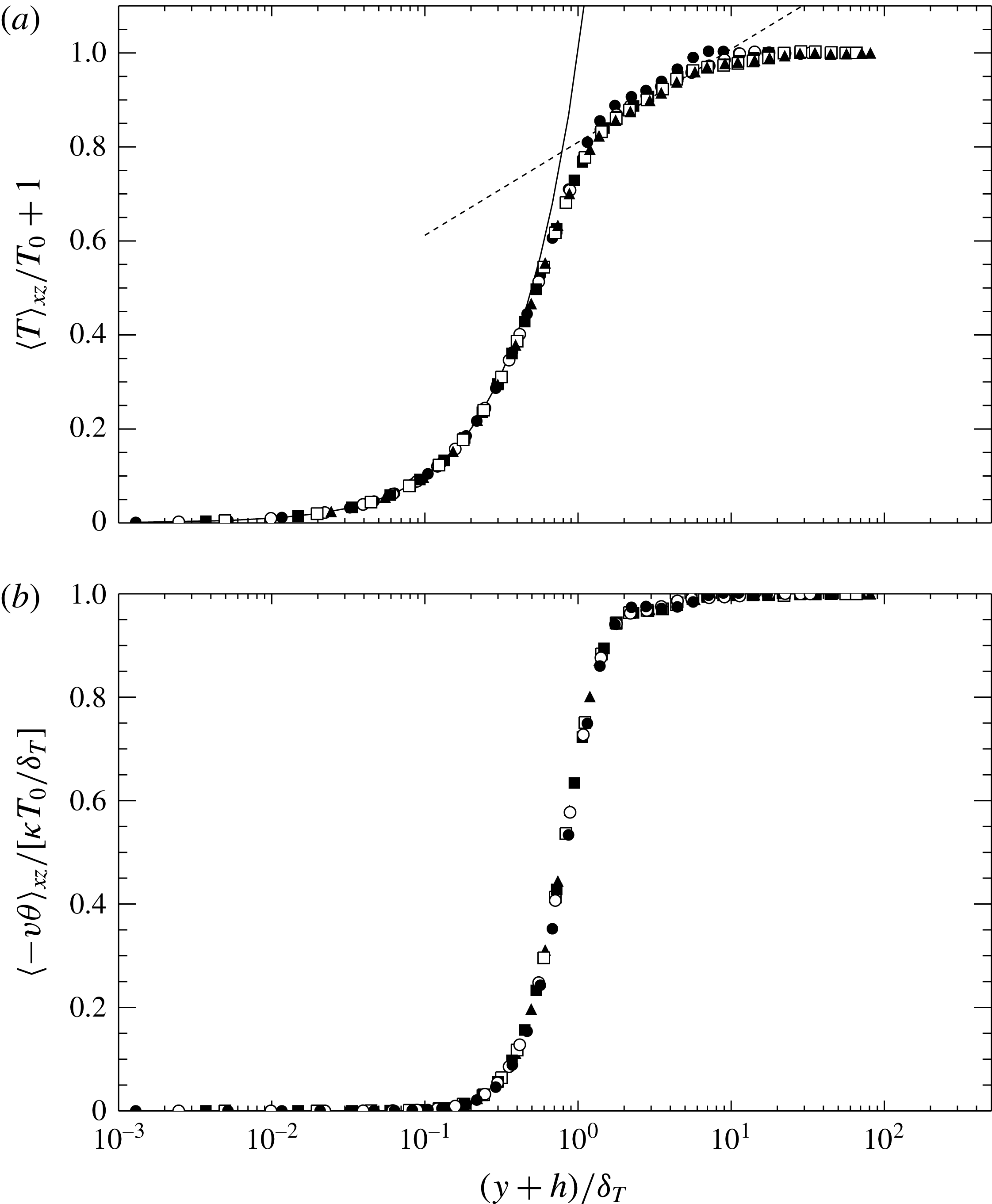
Figure 9 shows the mean temperature profile and the convective heat flux as a function of the distance to the wall,
 $(y+h)/\unicode[STIX]{x1D6FF}_{T}$
. At
 $(y+h)/\unicode[STIX]{x1D6FF}_{T}\ll 1$
, the mean temperature is expressed by
 $\langle T\rangle _{xz}/T_{0}+1=(y+h)/\unicode[STIX]{x1D6FF}_{T}$
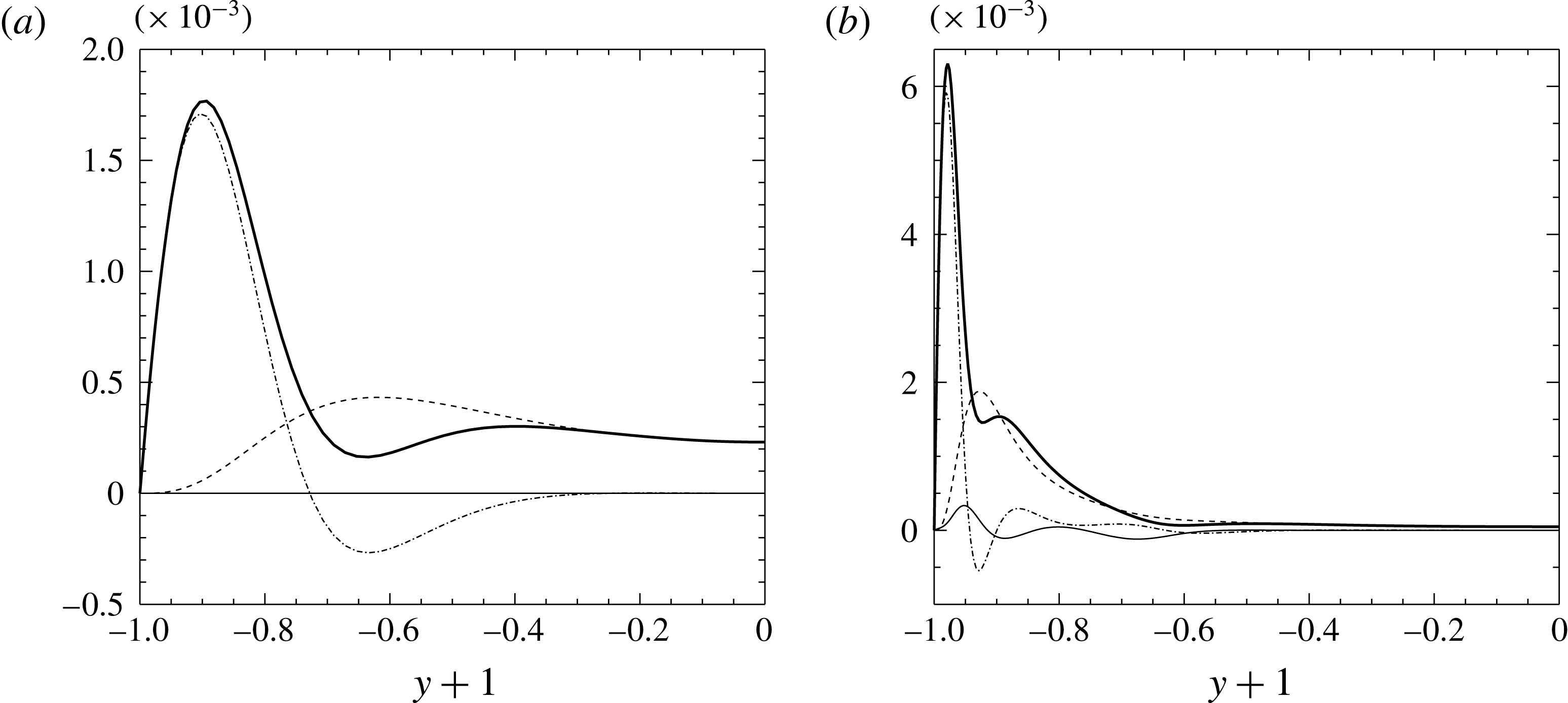
, since thermal conduction dominants over convection. Note that the total heat flux (the sum of the convective and conductive heat fluxes) is strictly unity at any height (see (2.7)). The convective and conductive heat fluxes are comparable around
 $(y+h)/\unicode[STIX]{x1D6FF}_{T}\approx 1$
. The convective heat flux is significant at
 $(y+h)/\unicode[STIX]{x1D6FF}_{T}\gtrsim 1$
. At
 $(y+h)/\unicode[STIX]{x1D6FF}_{T}\gtrsim 10$
there is almost no contribution from the conduction, i.e. no temperature gradient because of almost complete mixing of the scalar
 $T$
by the large-scale circulation. The hierarchical vortex structures lead to the logarithmic-like temperature profile in the intermediate region
 $1\lesssim (y+h)/\unicode[STIX]{x1D6FF}_{T}\lesssim 10$
. The dashed line represents the logarithmic fit
 $\langle T\rangle _{xz}/T_{0}+1=0.086\ln [(y+h)/\unicode[STIX]{x1D6FF}_{T}]+0.81$
determined in the range
 $1<(y+h)/\unicode[STIX]{x1D6FF}_{T}<10$
. It is well known that a logarithmic mean temperature profile appears as a consequence of heat transfer in near-wall turbulence where self-similar hierarchical vortical structures are commonly observed. Recently the logarithmic temperature distribution has also been found numerically and experimentally in thermal convection turbulence (Ahlers et al.
Reference Ahlers, Bodenschatz, Funfschilling, Grossmann, He, Lohse, Stevens and Verzicco2012; Ahlers, Bodenschatz & He Reference Ahlers, Bodenschatz and He2014).
6 Effects of flow three-dimensionality on local scalar dissipation
Scalar dissipation as a function of
 $Re$
for
 $\unicode[STIX]{x1D706}=0.1$
. Filled circles denote the scalar dissipation for the optimal state and open circles stand for that obtained from the optimisation only within a streamwise-independent two-dimensional velocity field.

The optimal flow fields for
 $\unicode[STIX]{x1D706}=0.1$
. (a)
 $Re=247.4$
, (b)
 $Re=247.5$
, (c)
 $Re=249$
. Light (or dark) grey objects represent isosurfaces of
 $\unicode[STIX]{x1D714}_{x}=+0.4$
(or
 $-0.4$
).

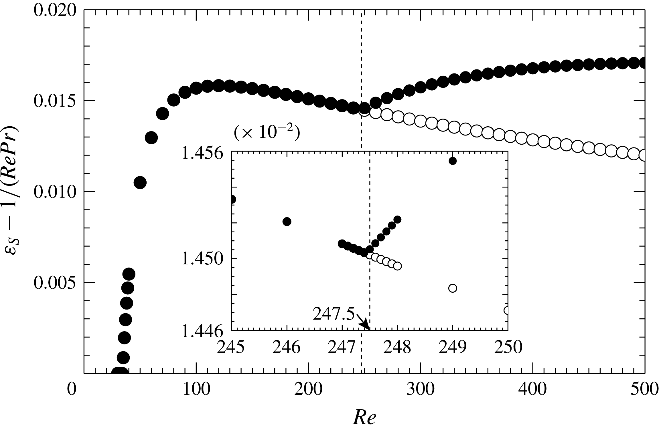
Figure 10 shows the scalar dissipation in the optimal state as a function of
 $Re$
for
 $\unicode[STIX]{x1D706}=0.1$
to present a bifurcation diagram of the solution to the Euler–Lagrange equation. The two-dimensional solution emerges from supercritical pitchfork bifurcation on the laminar solution at
 $Re=35$
. The two-dimensional solution exhibits a streamwise-independent velocity field representing a pair of streamwise convection rolls shown in figure 4(a,b), and satisfying two spatial symmetries
 $$\begin{eqnarray}\displaystyle & \displaystyle [u,v,w](x,y,z)=[u,v,-w](x,y,-z), & \displaystyle\end{eqnarray}$$
 $$\begin{eqnarray}\displaystyle & \displaystyle [u,v,w](x,y,z)=[-u,v,-w](x,-y,z). & \displaystyle\end{eqnarray}$$
As
 $Re$
increases further, the secondary pitchfork bifurcation occurs on the two-dimensional solution branch at
 $Re=247.5$
to create a three-dimensional solution with a shift-and-reflection symmetry
 $$\begin{eqnarray}\displaystyle \displaystyle [u,v,w](x,y,z)=[u,v,-w](x+L_{x}/2,y,-z), & & \displaystyle\end{eqnarray}$$
and the symmetry (6.2), which brings about the significantly higher scalar dissipation. When
 $\unicode[STIX]{x1D706}$
is changed, the corresponding bifurcation arises at different values of
 $Re$
, but the qualitative characteristics of the bifurcation diagram are not changed (the pitchfork bifurcation occurs at larger
 $Re$
as
 $\unicode[STIX]{x1D706}$
increases). Figure 11 shows the isosurface of the streamwise vorticity
 $\unicode[STIX]{x1D714}_{x}$
at the Reynolds numbers close to the onset of the three-dimensional solution,
 $Re=247.4,\,247.5$
and
 $249$
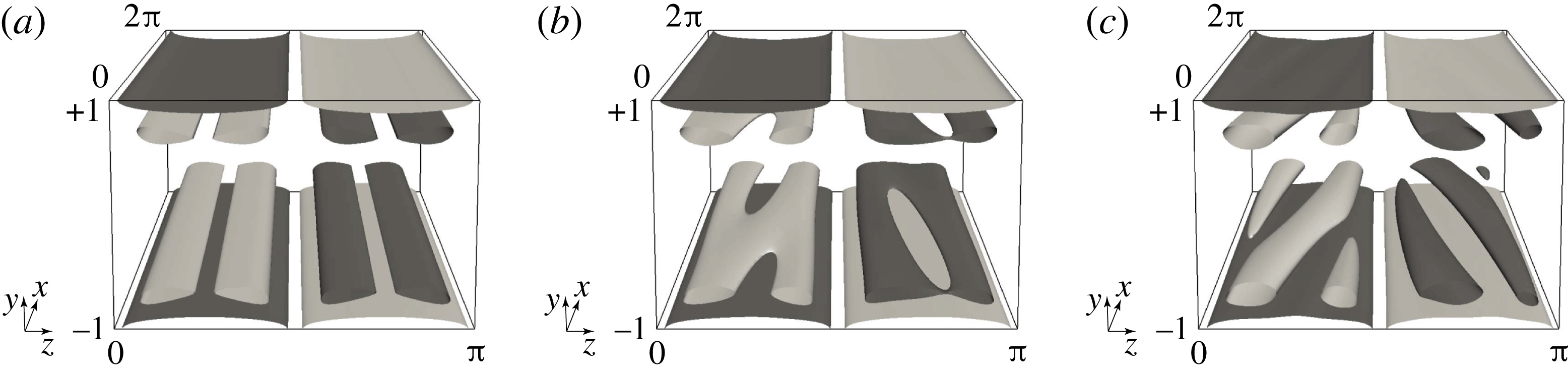
. As shown in figure 5, the optimal state has the streamwise large-scale circulation rolls. They generate sheet-like distribution of strong vorticity on the walls due to the no-slip condition, and just above the sheets the oppositely signed tube-like (or ribbon-like) streamwise vortices appear. At
 $Re=247.5$
, the near-wall tubular structures exhibit streamwise dependence, that is three-dimensionality. At
 $Re=249$
tubular vortices bear spanwise inclination as already seen in figure 4(c,d) at higher
 $Re$
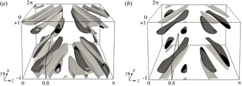
. It is important to recall that the scalar dissipation is enhanced with the appearance of the three-dimensional structures as shown in figure 10. Figure 12 visualises isosurfaces of a positive value of the second invariant of the velocity gradient tensor
 $$\begin{eqnarray}\displaystyle Q=-\frac{\unicode[STIX]{x2202}u_{i}}{\unicode[STIX]{x2202}x_{j}}\frac{\unicode[STIX]{x2202}u_{j}}{\unicode[STIX]{x2202}x_{i}} & & \displaystyle\end{eqnarray}$$
for the optimal state at
 $Re=249$
. The spanwise vorticity fluctuation
 $\unicode[STIX]{x1D714}_{z}^{\prime }=\unicode[STIX]{x1D714}_{z}-\langle \unicode[STIX]{x1D714}_{z}\rangle _{xz}$
is also shown on the
 $Q$
isosurfaces by grey scale. It can be seen that most of all the extracted tube-like structures exhibit
 $\unicode[STIX]{x1D714}_{z}^{\prime }>0$
. That is, the vortex tubes are tilted in the spanwise direction so that they may produce the spanwise vorticity antiparallel to the vorticity of the background shear flow. In the figures, the regions with significant increase of the local dissipation from the two-dimensional solution at the same value of
 $Re$
are also shown. The local scalar and energy dissipation are given respectively by
 $$\begin{eqnarray}\displaystyle D_{S}=\frac{1}{Re\,Pr}\left(\frac{\unicode[STIX]{x2202}\unicode[STIX]{x1D703}}{\unicode[STIX]{x2202}x_{j}}\right)^{2},\quad D_{E}=\frac{1}{Re}\left(\frac{\unicode[STIX]{x2202}u_{i}}{\unicode[STIX]{x2202}x_{j}}\right)^{2}, & & \displaystyle\end{eqnarray}$$
and thus it follows that
 $\langle D_{S}\rangle _{xyz}+1/(Re\,Pr)=\unicode[STIX]{x1D700}_{S}$
and
 $\langle D_{E}\rangle _{xyz}=\unicode[STIX]{x1D700}_{E}$
. In figure 12, the regions of
 $D_{E}-D_{E}^{\text{2D}}>0$
are found to appear just below the vortex tubes which are flanked with the regions of
 $D_{S}-D_{S}^{\text{2D}}>0$
, where the superscript 2D means the two-dimensional solution.
Vortical structures and significant increases in the local scalar and energy dissipation for the three-dimensional optimal velocity field against the two-dimensional optimal velocity field at
 $Re=249$
for
 $\unicode[STIX]{x1D706}=0.1$
. The dark grey (or black) objects represent isosurfaces,
 $Q=+0.03$
, of the second invariant of velocity gradient tensor, on which the positive (or negative) spanwise vorticity fluctuation
 $\unicode[STIX]{x1D714}_{z}^{\prime }$
are shown. Light grey objects indicate isosurfaces of (a) an increase in the local scalar dissipation,
 $D_{S}-D_{S}^{\text{2D}}=+0.001$
, (b) an increase in the local energy dissipation,
 $D_{E}-D_{E}^{\text{2D}}=+0.001$
. The frame in the figures indicates the plane
 $z=0.8$
.

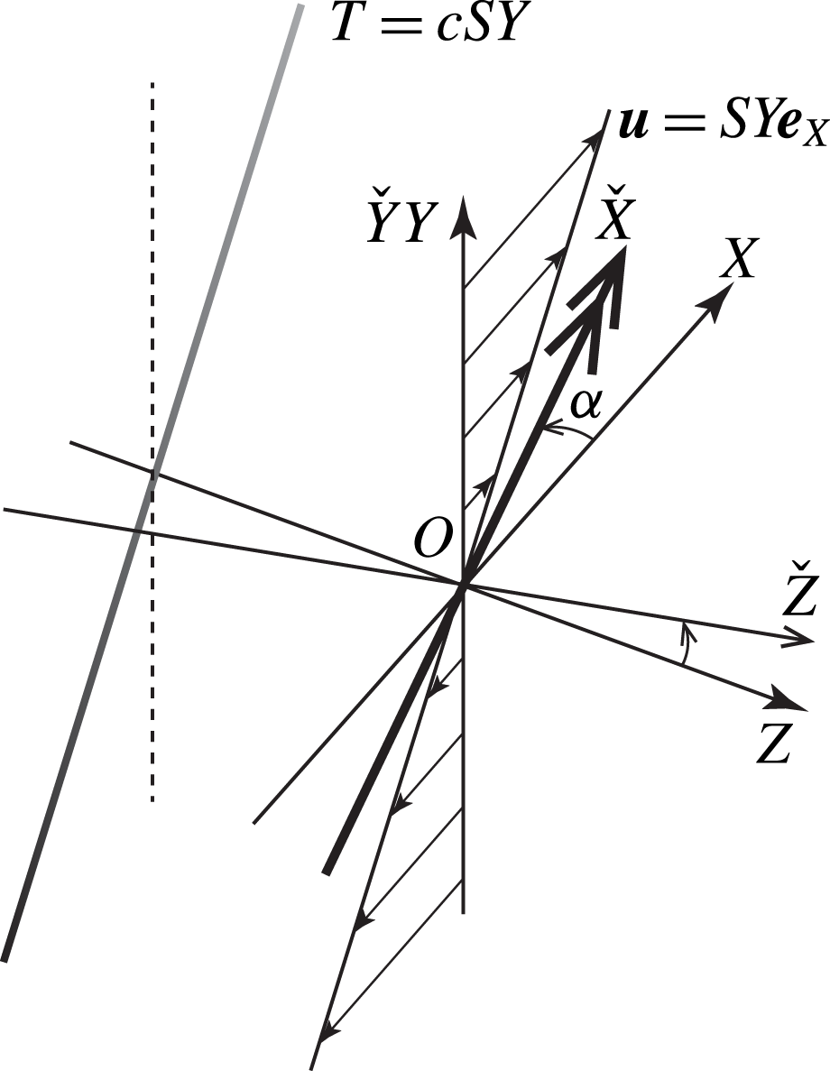
Illustration of scalar fields around cyclonic, neutral and anticyclonic vortex tubes in shear flow. (a,b,c) Configuration of the vortex tube in the shear flow. The vortex tube is inclined at an angle
 $\unicode[STIX]{x1D6FC}$
from the
 $X$
-axis on the plane
 $Y=0$
. (d,e,f) Isocontours of the scalar in the (
 ${\check{Z}}$
,
 $\check{Y}$
)-plane normal to the central axis of the vortex tube. (a,d) The cyclonic case (
 $\unicode[STIX]{x1D6FC}>0$
), (b,e) the neutral case (
 $\unicode[STIX]{x1D6FC}=0$
), (c,f) the anticyclonic case (
 $\unicode[STIX]{x1D6FC}<0$
).

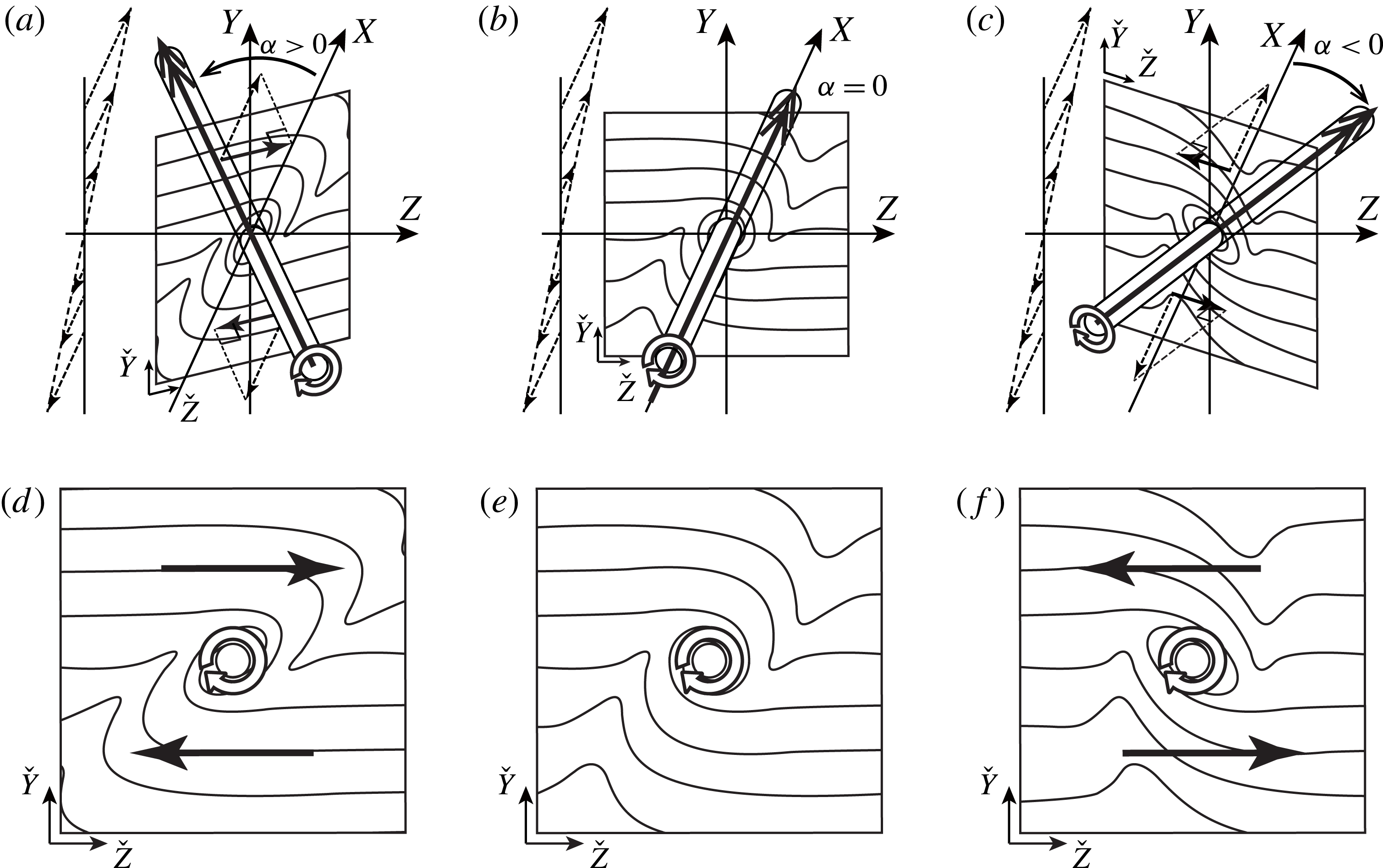
The mechanism responsible for the increase in the local scalar dissipation in the flanks of the tilted quasi-streamwise vortex tube can be explained in terms of the following simple model. Figure 13 shows illustrations of the scalar field around a vortex tube in shear flow. Suppose that the vortex tube is inclined at an angle
 $\unicode[STIX]{x1D6FC}$
from the streamwise (
 $X$
-) direction on the plane
 $Y=0$
. If
 $\unicode[STIX]{x1D6FC}>0$
(or
 $\unicode[STIX]{x1D6FC}<0$
), the vortex has the spanwise (
 $Z$
-) vorticity component with the same (or opposite) sign as that of the shear flow. Hereafter, the tilted vortex tubes of the same (or opposite) signed spanwise vorticity as that of the shear flow is referred to as a cyclonic (or anticyclonic) vortex. Figure 13(d,e,f) shows the isocontours of the scalar in the
 $(\check{Y},{\check{Z}})$
-plane normal to the central axis of the vortex tube. As illustrated in these figures, the vortex tube spirally wraps the isosurfaces of the scalar around itself through the convective transfer induced by swirling flow. For
 $\unicode[STIX]{x1D6FC}=0$
(figure 13
b,e), the shear flow has no effect on the scalar field because it is tangent to the scalar isosurfaces everywhere. In the case of
 $\unicode[STIX]{x1D6FC}\neq 0$
, however, the shear flow has the normal velocity component to the isosurfaces, and so it will play a distinct role in the convective scalar transfer depending on the sign of the inclination angle
 $\unicode[STIX]{x1D6FC}$
. When
 $\unicode[STIX]{x1D6FC}>0$
(i.e. the cyclonic inclination), the spacing of the wrapped isosurfaces of the scalar is widened by the cross-axial velocity component of the shear flow as shown in figure 13(a,d). As a result, the local scalar gradient is decreased around the vortex tube, and thus the scalar dissipation is reduced. On the other hand, when
 $\unicode[STIX]{x1D6FC}<0$
(i.e. the anticyclonic inclination), the spacing of the wrapped isosurfaces is tightened as shown in figure 13(c,f). It turns out that the scalar dissipation is locally intensified in the flanks of the anticyclonic vortex tubes, which have been observed in the optimal states at high Reynolds numbers. Note that although the scalar dissipation is enhanced in the lower left and upper right of the anticyclone in the above simple model (figure 13
d), in reality the higher scalar dissipation is observed in the lower position of the anticyclone, where the mean scalar gradient is much larger than in the upper position.
Appendix D analytically demonstrates this local effect of the anticyclonic inclination on the total scalar dissipation (or equivalently the wall heat flux in plane Couette flow) for a tilted diffusing vortex tube with circulation
 $\unicode[STIX]{x1D6E4}({>}0)$
in uniform shear flow of a shear rate
 $S({>}0)$
. In this flow system, using uniform temperature gradient
 $cS$
of an initial temperature field (
 $c$
is a constant whose dimension is temperature/velocity), the total scalar dissipation
 $\unicode[STIX]{x1D700}_{S}^{\ast }$
at early time
 $St|\unicode[STIX]{x1D6FC}|\ll 1$
and high vortex Péclet number
 $\unicode[STIX]{x1D6E4}/\unicode[STIX]{x1D705}\gg 1$
is evaluated analytically as
 $$\begin{eqnarray}\displaystyle \displaystyle \unicode[STIX]{x1D700}_{S}^{\ast }\approx {\unicode[STIX]{x1D700}_{S}^{\ast }|}_{\unicode[STIX]{x1D6FC}=0}-\unicode[STIX]{x1D6FC}\left[\frac{1}{4}\unicode[STIX]{x1D705}c^{2}S^{3}\unicode[STIX]{x1D6E4}\ln \left(\frac{\unicode[STIX]{x1D6E4}}{2\unicode[STIX]{x03C0}\unicode[STIX]{x1D705}}\right)t^{2}\right], & & \displaystyle\end{eqnarray}$$
where the leading-order term in the right-hand side represents the total scalar dissipation for a purely aligned vortex with the shear flow (
 $\unicode[STIX]{x1D6FC}=0$
). For the cyclonic case
 $\unicode[STIX]{x1D6FC}>0$
(or the anticyclonic case
 $\unicode[STIX]{x1D6FC}<0$
), the total scalar dissipation is reduced (or enhanced) in comparison with that of the neutral case of
 $\unicode[STIX]{x1D6FC}=0$
. This result has been obtained for self-similar diffusing vortex free from the presence of a wall; however, the essential physical mechanism proposed in figure 13 is thought to be valid even for the time-independent optimal state in a plane channel.
Two-dimensional cuts of the vorticity field, the velocity field, and the local scalar and energy dissipation fields at
 $Re=249$
for
 $\unicode[STIX]{x1D706}=0.1$
at
 $z=0.8$
. (a) Isocontours of the spanwise vorticity fluctuation
 $\unicode[STIX]{x1D714}_{z}^{\prime }$
and the velocity vectors
 $(u+1,v)$
relative to the lower moving wall in the plane
 $z=0.8$
shown in figure 12. (b) Isocontours of the second invariant of velocity gradient tensor
 $Q$
, (c) a difference in the local scalar dissipation
 $D_{S}-D_{S}^{2D}$
, (d) a difference in the local energy dissipation
 $D_{E}-D_{E}^{2D}$
in the plane
 $z=0.8$
.

Contributions from the four regions distinguished by the second invariant of the velocity gradient tensor
 $Q$
and the spanwise vorticity fluctuation
 $\unicode[STIX]{x1D714}_{z}^{\prime }$
to the total scalar dissipation for
 $\unicode[STIX]{x1D706}=0.1$
. Note that in (b),
 $\unicode[STIX]{x1D700}_{S,4}-2.85\times 10^{-3}$
is shown instead of
 $\unicode[STIX]{x1D700}_{S,4}$
.

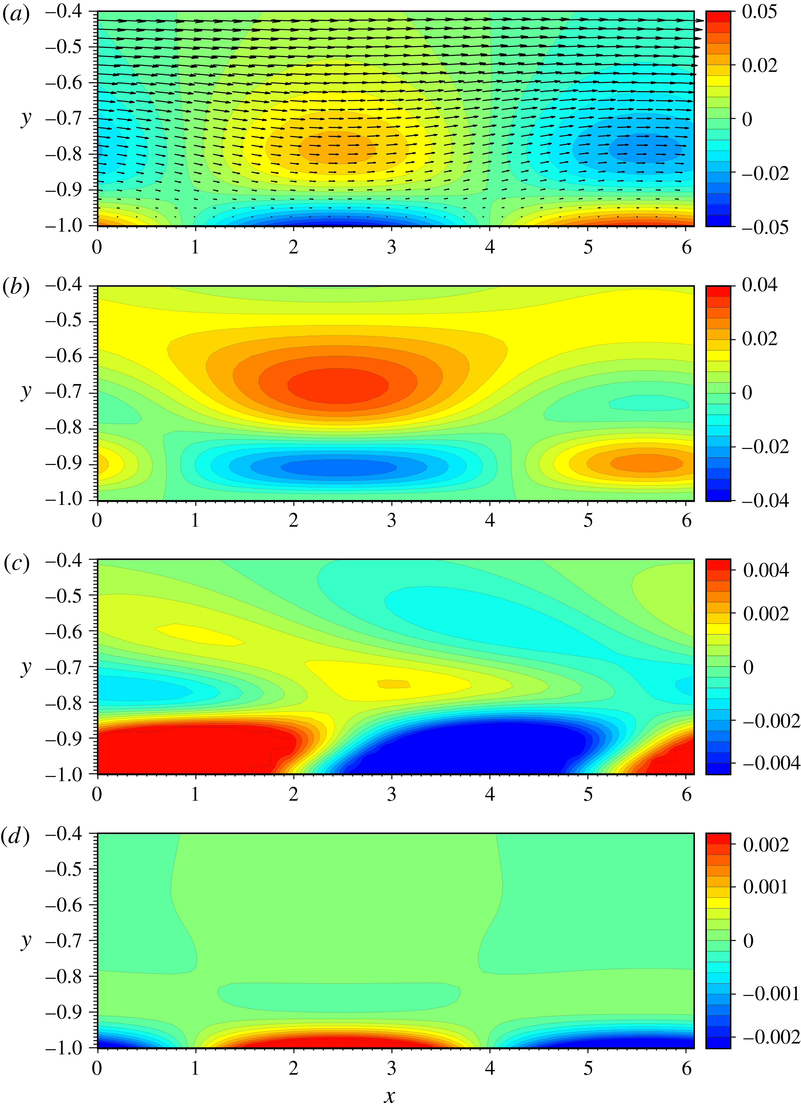
Besides, the near-wall vortex tube of the anticyclonic inclination has another role in heat transfer enhancement, which will be more significant at higher Reynolds numbers. Figures 4(a)–4(d) respectively show the isocontours of
 $\unicode[STIX]{x1D714}_{z}^{\prime }$
,
 $Q$
,
 $D_{S}-D_{S}^{\text{2D}}$
and
 $D_{E}-D_{E}^{\text{2D}}$
at
 $Re=249$
. Figure 14(a) shows the velocity vectors relative to the lower wall in the (
 $x,y$
)-plane. The anticyclonic vortex of
 $\unicode[STIX]{x1D714}_{z}^{\prime }>0$
is found around
 $(x,y)=(2.4,-0.7)$
. In figure 14(c), the higher scalar dissipation can be observed in the downstream (or right-hand side) flank of the vortex. This local enhancement of
 $D_{S}$
is attributed to the above-described tightening of wrapped isotherms by the cross-axial shear flow just downstream (larger
 $x$
) of the anticyclonic vortex. On the other hand, the anticyclonic vortex induces the downward flow towards the lower wall upstream of (or in the left-hand side of) the vortex. The symmetric counterpart of this near-wall vortex exists on the upper wall as well. The high- (or low-) temperature fluid is pushed on the lower cold (or upper hot) wall by the near-wall anticyclonic vortex, leading to a large temperature gradient near the walls. As a result, the local scalar dissipation is significantly increased near the wall upstream of the anticyclonic vortices. The distribution of
 $D_{E}$
is much differ from
 $D_{S}$
(cf. figure 14
c,d). The local energy dissipation is significantly increased just below the anticyclonic vortex due to the no-slip boundary condition.
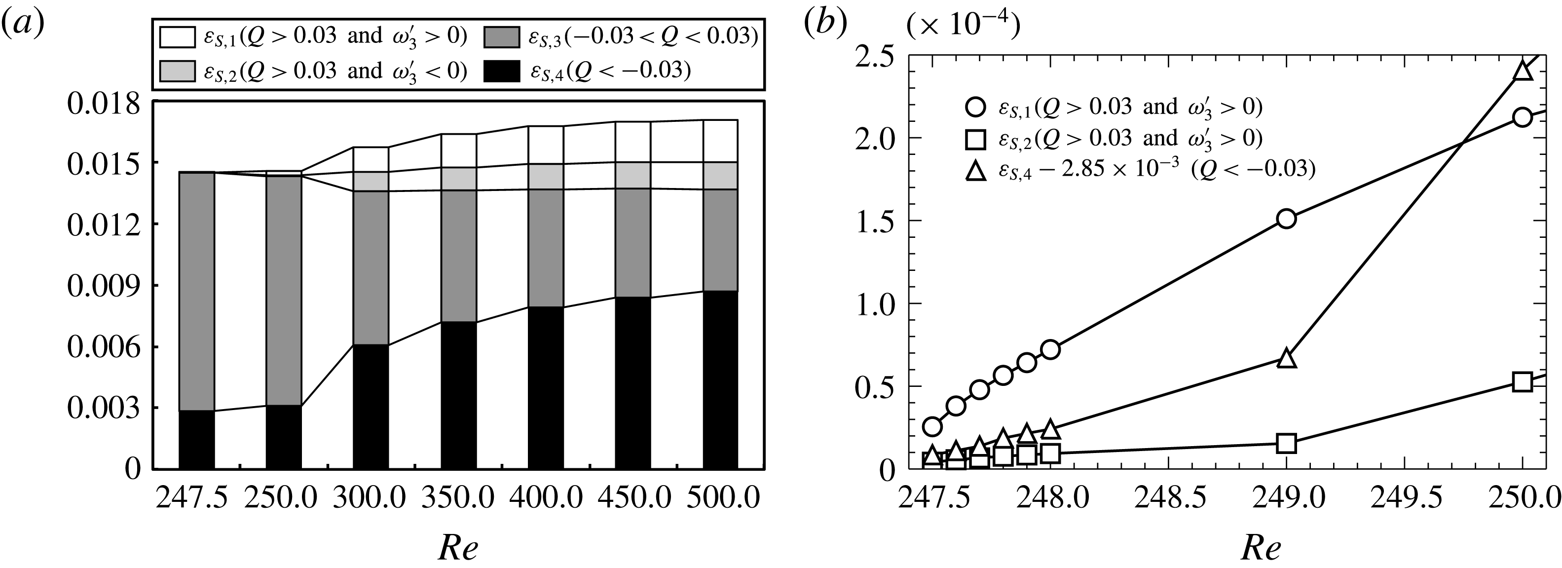
Figure 15 shows the fractional contribution to the total scalar dissipation. Each contribution represents the integration over one of the separated four regions by using
 $Q$
and
 $\unicode[STIX]{x1D714}_{z}^{\prime }$
, defined as
 $$\begin{eqnarray}\displaystyle \displaystyle \unicode[STIX]{x1D700}_{S,n}=\frac{1}{Re\,Pr\,V}\int _{\unicode[STIX]{x1D6FA}_{n}}\left(\frac{\unicode[STIX]{x2202}\unicode[STIX]{x1D703}}{\unicode[STIX]{x2202}x_{j}}\right)^{2}\text{d}V\hspace{20.00003pt}(n=1,2,3,4), & & \displaystyle\end{eqnarray}$$
where
 $\unicode[STIX]{x1D6FA}_{1}$
,
 $\unicode[STIX]{x1D6FA}_{2}$
,
 $\unicode[STIX]{x1D6FA}_{3}$
and
 $\unicode[STIX]{x1D6FA}_{4}$
denote the anticyclonic region of
 $Q>0.03$
and
 $\unicode[STIX]{x1D714}_{z}^{\prime }>0$
, the cyclonic region of
 $Q>0.03$
and
 $\unicode[STIX]{x1D714}_{z}^{\prime }<0$
, the shear region with
 $|Q|<0.03$
(i.e. comparable vorticity and strain), and the strain region of
 $Q<-0.03$
, respectively. Note that
 $\unicode[STIX]{x1D700}_{S}=\unicode[STIX]{x1D700}_{S,1}+\unicode[STIX]{x1D700}_{S,2}+\unicode[STIX]{x1D700}_{S,3}+\unicode[STIX]{x1D700}_{S,4}+1/(Re\,Pr)$
.
 $\unicode[STIX]{x1D700}_{S,3}$
is dominant at
 $Re=247.5$
and
 $Re=250$
(figure 18
a). The main contributor to
 $\unicode[STIX]{x1D700}_{S,3}$
is the near-wall ‘impinging jet’ in between the large-scale circulation rolls, which significantly increases the heat flux on the walls as in the case of thermal convection. This contribution is, however, decreased as
 $Re$
increases. Immediately after the bifurcation of the three-dimensional optimal field from the two-dimensional branch,
 $\unicode[STIX]{x1D700}_{S,1}$
and
 $\unicode[STIX]{x1D700}_{S,4}$
are remarkably increased as shown in figure 15(b). These are consequences of the anticyclonic inclination of the streamwise vortex tubes leading to the local enhancement of the temperature gradient by the cross-axial mean shear around the anticyclonic tube as well as by the tube-induced flow towards the wall, in the vicinity of which the strong strain arises. At large Reynolds numbers
 $\unicode[STIX]{x1D700}_{S,4}$
becomes dominant.
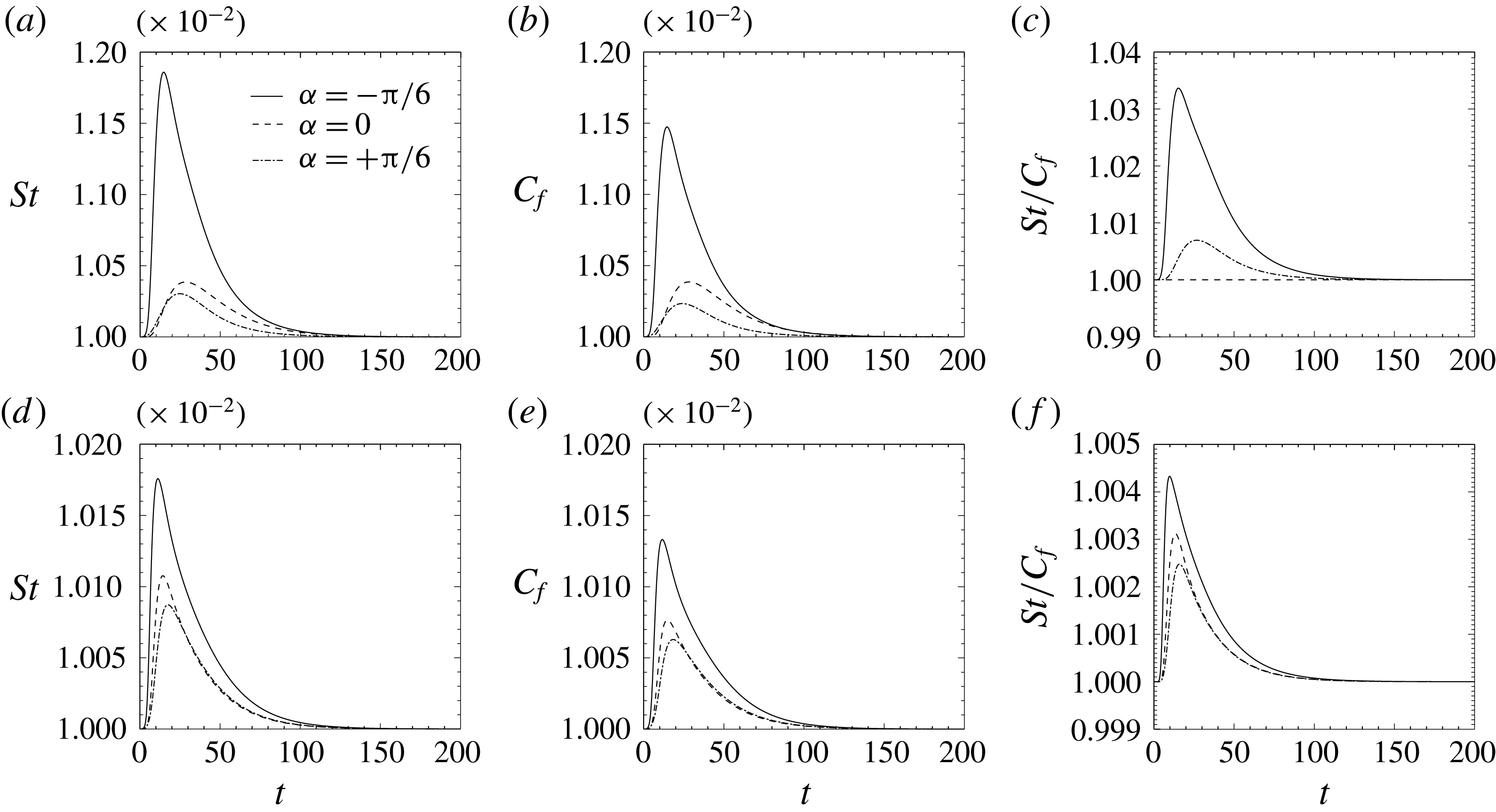
Appendix E numerically demonstrates that the introduction of an anticyclonic quasi-streamwise vortex leads to significant heat transfer enhancement in comparison to that of a cyclonic or purely streamwise vortex even in the Navier–Stokes system without any external force, and that the introduced vortices and their effect are robust against a finite-amplitude three-dimensional disturbance.
7 Summary and discussion
We have explored optimal heat transfer enhancement in plane Couette flow. Optimal time-independent velocity fields have been found by maximisation of an objective functional defined as the excess of a wall heat flux (total scalar dissipation) over total energy dissipation under the constraint of incompressibility of the velocity and an advection-diffusion equation for temperature. At quite a low Reynolds number
 $Re\sim 10^{0}$
, an optimal state is laminar flow, but non-trivial solutions appear at a higher Reynolds number
 $Re\sim 10^{1}$
. We have obtained a streamwise-independent two-dimensional field as an optimal state. The velocity field consists of large-scale circulation rolls that play a role in heat transfer enhancement with respect to laminar conductive heat transfer as in thermal convection. A three-dimensional optimal state has been observed to arise from pitchfork bifurcation on the two-dimensional branch at
 $Re\sim 10^{2}$
. The three-dimensional velocity field possesses similar large-scale rolls to those in the two-dimensional solutions; however, small-scale quasi-streamwise vortex tubes appear near the walls to be tilted in the spanwise direction from the streamwise direction. The velocity fields exhibit extremely high performance for heat transfer enhancement even at much higher Reynolds numbers
 $Re\sim 10^{3}$
. In the optimal states, higher scalar dissipation (i.e. a higher wall heat flux) is achieved with less energy dissipation than the time-averaged dissipation in a corresponding turbulent state.
In the three-dimensional optimal state at high
 $Re$
, the spanwise spacing of the quasi-streamwise vortex tubes near the wall is proportionate to their distance from the wall. The spacing of the largest vortices, i.e. the large-scale circulation rolls, scales with the outer length (i.e. channel half-width
 $h$
), and it is independent of
 $Re$
. On the other hand, the spacing of the smallest vortex scales with the inner length which is given by the temperature difference and the temperature gradient on the wall. We have observed quasi-streamwise vortical structures with hierarchical self-similarity up to the distance from the wall,
 $0.2h$
. Interestingly, the hierarchical structure leads to a logarithmic-like mean temperature profile in the region in which a convective heat flux is dominant.
We have presented the two mechanisms for heat transfer enhancement in the three-dimensional optimal state in comparison to the streamwise-independent two-dimensional state. The quasi-streamwise vortex tubes incline in the opposite direction to the vorticity of the mean shear flow. This anticyclonic inclination of the vortex tubes brings about a remarkable increase in the local and thus total scalar dissipation. The isotherms wrapped around the anticyclonic vortices undergo the cross-axial mean shear, so that the spacing of the wrapped isotherms is narrower and so the temperature gradient is steeper than those around a purely streamwise (two-dimensional) vortex tube, intensifying scalar dissipation and so a wall heat flux. The high-Péclet-number and early-time asymptotic analysis of the simple analytical model for a tilted straight vortex tube in uniform shear flow demonstrates that the intensification of the local scalar dissipation around the vortex tube leads to an increase in total scalar dissipation. Moreover, the tilted anticyclonic vortices highly induce the flow towards the wall to push low- (or high-) temperature fluids on the hot (or cold) wall, enhancing the wall heat flux. In wall turbulence and uniformly sheared turbulence, however, streamwise vortices have often been observed to incline in the cyclonic direction rather than in the anticyclonic direction. In real heat transfer enhancement of turbulent shear flows, therefore, the introduction of an anticyclonic inclination of quasi-streamwise vortices could be new passive control strategy for heat transfer enhancement. As shown in appendix E, our supplemental numerical simulations for the introduction of an axially uniform (two-dimensional) as well as axially non-uniform (three-dimensional) anticyclonic quasi-streamwise vortex tubes in laminar plane Couette flow has confirmed significant dissimilar heat transfer enhancement in comparison to that of a cyclonic or purely streamwise vortex even in the time-dependent Navier–Stokes system without any external forcing. Although the observed heat transfer enhancement is transient, we can sustain the enhancement by introducing the vortices periodically. This result demonstrates that the simple strategy inspired by the essence of the optimised velocity fields really works well for heat transfer enhancement.
Another approach to enhancement of the dissimilarity between heat and momentum transfer is to optimally control the flow governed by the Navier–Stokes equation without dissimilar external force. In their numerical experiments of turbulent channel flow, Yamamoto et al. (Reference Yamamoto, Hasegawa and Kasagi2013) have introduced blowing and suction on the wall to optimise the ratio between the Stanton number and the friction coefficient by computing the adjoint velocity and temperature fields during a certain time interval in the past. They have observed a roughly spanwise-independent travelling-wave-like velocity field in their controlled flow. The optimal states found in this work are the outcomes of pursuing an incompressible velocity field which achieves more wall heat flux and less total energy dissipation without imposing the Navier–Stokes constraint, and therefore they are distinct from the dissimilar state observed by Yamamoto et al. (Reference Yamamoto, Hasegawa and Kasagi2013).
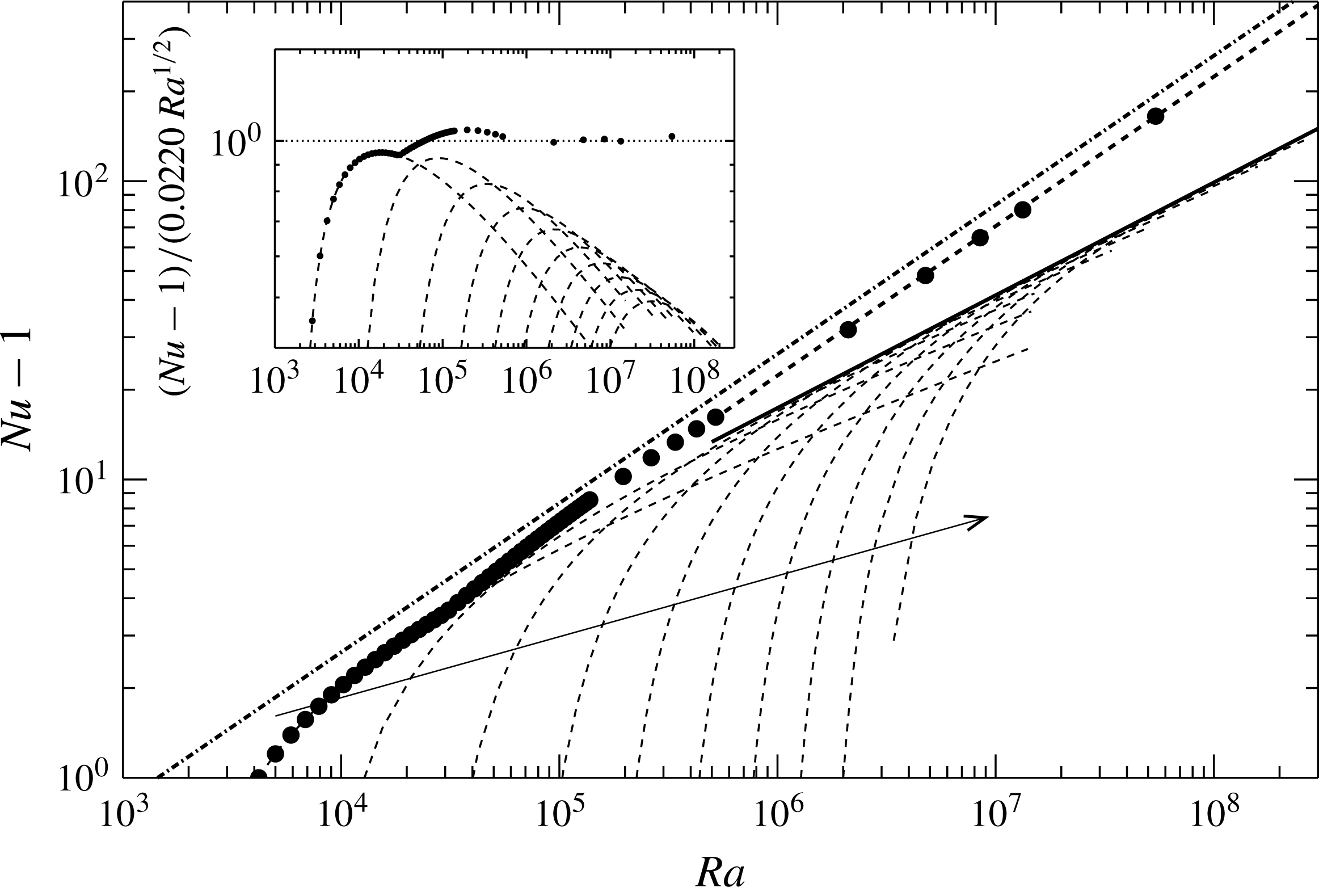
Nusselt number
 $Nu$
as a function of Rayleigh number
 $Ra$
. Symbols denote the optimal state for
 $\unicode[STIX]{x1D706}=0.1$
. The thick dashed line shows the power fit
 $Nu-1=0.0220Ra^{0.501}$
determined in the range
 $5\times 10^{5}<Ra<6\times 10^{7}$
. The dashed curves stand for the values optimised only within a streamwise-independent two-dimensional velocity field of the aspect ratio
 $L_{z}/L_{y}=\unicode[STIX]{x03C0}/2,\unicode[STIX]{x03C0}/4,\unicode[STIX]{x03C0}/6,\unicode[STIX]{x03C0}/8,\unicode[STIX]{x03C0}/10,\unicode[STIX]{x03C0}/12,\unicode[STIX]{x03C0}/14,\unicode[STIX]{x03C0}/16,\unicode[STIX]{x03C0}/18$
and
 $\unicode[STIX]{x03C0}/20$
along the arrow. The thick solid line indicates the envelope fit
 $Nu-1=0.0937Ra^{0.378}$
determined in the range
 $10^{7}<Ra<10^{8}$
. The dash-dotted line represents the upper bound in the Rayleigh–Bénard convection with the no-slip boundary condition,
 $Nu-1=0.02634Ra^{1/2}$
(Plasting & Kerswell Reference Plasting and Kerswell2003). The inset shows the compensated
 $Nu$
.

Hassanzadeh et al. (Reference Hassanzadeh, Chini and Doering2014) have recently reported time-independent optimal states for two-dimensional convection between two parallel impermeable but free-slip plates of a constant temperature difference by maximising a heat flux under the three constraints: divergence-free velocity field, temperature field satisfying an advection-diffusion equation, and fixed enstrophy. They related their optimal states to the Rayleigh–Bénard convection problem, and found the scaling of the Nusselt number
 $Nu$
with the Rayleigh number
 $Ra$
as
 $Nu\sim Ra^{5/12}$
, which agrees with the upper bounds in the case of the free-slip boundary condition, derived by the background method (Ierley, Kerswell & Plasting Reference Ierley, Kerswell and Plasting2006; Whitehead & Doering Reference Whitehead and Doering2012). Let us make a similar estimate for the optimal states obtained in the present study. For the combined natural and forced convection in plane Couette flow, the total energy budget equation is given by
 $$\begin{eqnarray}\displaystyle \displaystyle 8Re^{3}Pr^{2}(2\unicode[STIX]{x1D700}_{E}-C_{f})=Ra(Nu-1). & & \displaystyle\end{eqnarray}$$
By estimating
 $Ra$
from
 $\unicode[STIX]{x1D700}_{E}$
,
 $C_{f}$
and
 $Nu=(Re\,Pr/2)St$
in the present optimal states, we have found the scaling of
 $Nu$
with
 $Ra$
as
 $Nu\sim Ra^{1/2}$
for the three-dimensional optimal state at
 $Re=10^{3}-10^{4}$
, or equivalently
 $Ra=5\times 10^{5}-6\times 10^{7}$
(see figure 16). The observed exponent
 $1/2$
of
 $Ra$
is consistent with the scaling of the upper bound in the Rayleigh–Bénard convection with the no-slip boundary condition (Doering & Constantin Reference Doering and Constantin1996; Plasting & Kerswell Reference Plasting and Kerswell2003), and also accords with Kolmogorov’s scaling law of the turbulent energy dissipation, that is
 $\unicode[STIX]{x1D700}_{E}=\text{const}.$
as
 $Re\rightarrow \infty$
. As shown in figure 7(b), the optimal state at large
 $Re$
achieves nearly constant scalar and energy dissipation, and it exhibits a velocity field accommodating hierarchical vortical structures as discussed in § 5. Recently, Tobasco & Doering (Reference Tobasco and Doering2017) have reported that a two-dimensional velocity field satisfying no-slip boundary conditions and exhibiting hierarchical self-similar structure is able to achieve the ultimate asymptotic scaling
 $Nu\sim Ra^{1/2}$
in the time-independent maximal heat transfer problem for fixed enstrophy constraint. These results suggest that a certain class of hierarchical self-similar velocity fields might lead to the ultimate asymptotic scaling.
Acknowledgements
We are grateful to Professor C. R. Doering at University of Michigan for useful discussions. This work was partially supported by a Grant-in-Aid Scientific Research (grant nos. 25249014, 26630055) from the Japanese Society for Promotion of Science (JSPS). S.M. is supported by JSPS Grant-in-Aid for JSPS Fellows Grant Number 16J00685. This research partly used computational resources under Collaborative Research Program for Young Scientists provided by Academic Center for Computing and Media Studies, Kyoto University.
Appendix A. Numerical details
A.1 Discretisation of Euler–Lagrange equations
Since (3.2) implies that
 $$\begin{eqnarray}\frac{\unicode[STIX]{x2202}u_{i}^{new}}{\unicode[STIX]{x2202}x_{i}}=\frac{\unicode[STIX]{x2202}u_{i}}{\unicode[STIX]{x2202}x_{i}}+s\frac{\unicode[STIX]{x2202}\widehat{u}_{i}}{\unicode[STIX]{x2202}x_{i}}=s\frac{\unicode[STIX]{x2202}\widehat{u}_{i}}{\unicode[STIX]{x2202}x_{i}},\end{eqnarray}$$
in order that
 $\boldsymbol{u}^{new}$
is incompressible we invoke the continuity for
 $\widehat{\boldsymbol{u}}$
,
 $$\begin{eqnarray}\frac{\unicode[STIX]{x2202}\widehat{u}_{i}}{\unicode[STIX]{x2202}x_{i}}=0.\end{eqnarray}$$
Taking the double curl, the single curl and the
 $xz$
-average of (2.27), we have the equations for the wall-normal velocity
 $v$
, the wall-normal vorticity
 $\unicode[STIX]{x1D714}_{y}$
and the averaged velocities,
 $$\begin{eqnarray}\displaystyle & \displaystyle \frac{\unicode[STIX]{x2202}^{2}\widehat{v}}{\unicode[STIX]{x2202}x_{j}^{2}}=\frac{1}{Re}\frac{\unicode[STIX]{x2202}^{2}}{\unicode[STIX]{x2202}x_{j}^{2}}\frac{\unicode[STIX]{x2202}^{2}v}{\unicode[STIX]{x2202}x_{j}^{2}}+\unicode[STIX]{x1D706}H_{v}+\unicode[STIX]{x1D706}\left(\frac{\unicode[STIX]{x2202}^{2}}{\unicode[STIX]{x2202}x^{2}}+\frac{\unicode[STIX]{x2202}^{2}}{\unicode[STIX]{x2202}z^{2}}\right)\unicode[STIX]{x1D703}^{\ast }, & \displaystyle\end{eqnarray}$$
 $$\begin{eqnarray}\displaystyle & \displaystyle \widehat{\unicode[STIX]{x1D714}}_{y}=\frac{1}{Re}\frac{\unicode[STIX]{x2202}^{2}\unicode[STIX]{x1D714}_{y}}{\unicode[STIX]{x2202}x_{j}^{2}}+\unicode[STIX]{x1D706}H_{\unicode[STIX]{x1D714}}, & \displaystyle\end{eqnarray}$$
 $$\begin{eqnarray}\displaystyle & \displaystyle \langle \widehat{u}\rangle _{xz}=\frac{1}{Re}\frac{\text{d}^{2}\langle u\rangle _{xz}}{\text{d}y^{2}}+\unicode[STIX]{x1D706}\left\langle \unicode[STIX]{x1D703}^{\ast }\frac{\unicode[STIX]{x2202}\unicode[STIX]{x1D703}}{\unicode[STIX]{x2202}x}\right\rangle _{xz}, & \displaystyle\end{eqnarray}$$
 $$\begin{eqnarray}\displaystyle & \displaystyle \langle \widehat{w}\rangle _{xz}=\frac{1}{Re}\frac{\text{d}^{2}\langle w\rangle _{xz}}{\text{d}y^{2}}+\unicode[STIX]{x1D706}\left\langle \unicode[STIX]{x1D703}^{\ast }\frac{\unicode[STIX]{x2202}\unicode[STIX]{x1D703}}{\unicode[STIX]{x2202}z}\right\rangle _{xz}, & \displaystyle\end{eqnarray}$$
with
 $$\begin{eqnarray}\displaystyle & \displaystyle H_{v}=-\frac{\unicode[STIX]{x2202}}{\unicode[STIX]{x2202}y}\left[\frac{\unicode[STIX]{x2202}}{\unicode[STIX]{x2202}x}\left(\unicode[STIX]{x1D703}^{\ast }\frac{\unicode[STIX]{x2202}\unicode[STIX]{x1D703}}{\unicode[STIX]{x2202}x}\right)+\frac{\unicode[STIX]{x2202}}{\unicode[STIX]{x2202}z}\left(\unicode[STIX]{x1D703}^{\ast }\frac{\unicode[STIX]{x2202}\unicode[STIX]{x1D703}}{\unicode[STIX]{x2202}z}\right)\right]+\left(\frac{\unicode[STIX]{x2202}^{2}}{\unicode[STIX]{x2202}x^{2}}+\frac{\unicode[STIX]{x2202}^{2}}{\unicode[STIX]{x2202}z^{2}}\right)\left(\unicode[STIX]{x1D703}^{\ast }\frac{\unicode[STIX]{x2202}\unicode[STIX]{x1D703}}{\unicode[STIX]{x2202}y}\right), & \displaystyle\end{eqnarray}$$
 $$\begin{eqnarray}\displaystyle & \displaystyle H_{\unicode[STIX]{x1D714}}=\frac{\unicode[STIX]{x2202}}{\unicode[STIX]{x2202}z}\left(\unicode[STIX]{x1D703}^{\ast }\frac{\unicode[STIX]{x2202}\unicode[STIX]{x1D703}}{\unicode[STIX]{x2202}x}\right)-\frac{\unicode[STIX]{x2202}}{\unicode[STIX]{x2202}x}\left(\unicode[STIX]{x1D703}^{\ast }\frac{\unicode[STIX]{x2202}\unicode[STIX]{x1D703}}{\unicode[STIX]{x2202}z}\right), & \displaystyle\end{eqnarray}$$
from which
 $p^{\ast }$
has been eliminated. The corresponding boundary conditions are
 $$\begin{eqnarray}\displaystyle & \displaystyle v(y=\pm 1)=\frac{\unicode[STIX]{x2202}v}{\unicode[STIX]{x2202}y}(y=\pm 1)=0, & \displaystyle\end{eqnarray}$$
 $$\begin{eqnarray}\displaystyle & \displaystyle \unicode[STIX]{x1D714}_{y}(y=\pm 1)=0, & \displaystyle\end{eqnarray}$$
 $$\begin{eqnarray}\displaystyle & \displaystyle \langle u\rangle _{xz}(y=\pm 1)=\pm 1, & \displaystyle\end{eqnarray}$$
 $$\begin{eqnarray}\displaystyle & \displaystyle \langle w\rangle _{xz}(y=\pm 1)=0, & \displaystyle\end{eqnarray}$$
 $$\begin{eqnarray}\displaystyle & \displaystyle \unicode[STIX]{x1D703}(y=\pm 1)=0, & \displaystyle\end{eqnarray}$$
 $$\begin{eqnarray}\displaystyle & \displaystyle \unicode[STIX]{x1D703}^{\ast }(y=\pm 1)=0. & \displaystyle\end{eqnarray}$$
In the periodic streamwise and spanwise directions,
 $\boldsymbol{u}$
, vorticity
 $\unicode[STIX]{x1D74E}=\unicode[STIX]{x1D735}\times \boldsymbol{u}$
,
 $\unicode[STIX]{x1D703}$
and
 $\unicode[STIX]{x1D703}^{\ast }$
are approximated by truncated Fourier series
 $$\begin{eqnarray}\displaystyle (\boldsymbol{u},\unicode[STIX]{x1D74E},\unicode[STIX]{x1D703},\unicode[STIX]{x1D703}^{\ast }) & = & \displaystyle \mathop{\sum }_{k=-K}^{K}\mathop{\sum }_{m=-M}^{M}(\widetilde{\boldsymbol{u}}^{km},\widetilde{\unicode[STIX]{x1D74E}}^{km},\widetilde{\unicode[STIX]{x1D703}}^{km},\widetilde{\unicode[STIX]{x1D703}^{\ast }}^{km})\text{e}^{\text{i}2\unicode[STIX]{x03C0}kx/L_{x}}\text{e}^{\text{i}2\unicode[STIX]{x03C0}mz/L_{z}},\end{eqnarray}$$
where
 $K$
and
 $M$
are positive integers. Note that the Fourier coefficients of
 $u$
and
 $w$
for
 $(k,m)\neq (0,0)$
are given by
 $\widetilde{v}^{km}$
and
 $\widetilde{\unicode[STIX]{x1D714}_{y}}^{km}$
through
 $$\begin{eqnarray}\displaystyle & \displaystyle \widetilde{u}^{km}=\text{i}\frac{(2\unicode[STIX]{x03C0}k/L_{x})\text{d}\widetilde{v}^{km}/\text{d}y+(2\unicode[STIX]{x03C0}m/L_{z})\widetilde{\unicode[STIX]{x1D714}_{y}}^{km}}{4\unicode[STIX]{x03C0}^{2}(k^{2}/L_{x}^{2}+m^{2}/L_{z}^{2})}, & \displaystyle\end{eqnarray}$$
 $$\begin{eqnarray}\displaystyle & \displaystyle \widetilde{w}^{km}=\text{i}\frac{(2\unicode[STIX]{x03C0}m/L_{z})\text{d}\widetilde{v}^{km}/\text{d}y+(2\unicode[STIX]{x03C0}k/L_{x})\widetilde{\unicode[STIX]{x1D714}_{y}}^{km}}{4\unicode[STIX]{x03C0}^{2}(k^{2}/L_{x}^{2}+m^{2}/L_{z}^{2})}. & \displaystyle\end{eqnarray}$$
In the wall-normal direction,
 $\widetilde{v}^{km}$
,
 $\widetilde{\unicode[STIX]{x1D714}_{y}}^{km}$
,
 $\langle u\rangle _{xz}-y$
,
 $\langle w\rangle _{xz}$
,
 $\widetilde{\unicode[STIX]{x1D703}}^{km}$
and
 $\widetilde{\unicode[STIX]{x1D703}^{\ast }}^{km}$
are expanded, in terms of the polynomials which satisfy boundary conditions (A 9), as
 $$\begin{eqnarray}\displaystyle & \displaystyle \widetilde{v}^{km}=\mathop{\sum }_{n=0}^{N-4}c_{v}^{kmn}\left(T_{n}-2\frac{n+2}{n+3}T_{n+2}+\frac{n+1}{n+3}T_{n+4}\right), & \displaystyle\end{eqnarray}$$
 $$\begin{eqnarray}\displaystyle & \displaystyle (\widetilde{\unicode[STIX]{x1D714}_{y}}^{km},\widetilde{\unicode[STIX]{x1D703}}^{km},\widetilde{\unicode[STIX]{x1D703}^{\ast }}^{km})=\mathop{\sum }_{n=0}^{N-2}(c_{\unicode[STIX]{x1D714}}^{kmn},c_{\unicode[STIX]{x1D703}}^{kmn},c_{\unicode[STIX]{x1D703}^{\ast }}^{kmn})(T_{n}-T_{n+2}), & \displaystyle\end{eqnarray}$$
 $$\begin{eqnarray}\displaystyle (\langle u\rangle _{xz}-y,\langle w\rangle _{xz}) & = & \displaystyle \frac{3}{2}(\langle u\rangle _{xyz},\langle w\rangle _{xyz})(1-y^{2})\nonumber\\ \displaystyle & & \displaystyle +\,\frac{\text{d}}{\text{d}y}\left\{\mathop{\sum }_{n=0}^{N-4}(c_{u}^{n},c_{w}^{n})\left(T_{n}-2\frac{n+2}{n+3}T_{n+2}+\frac{n+1}{n+3}T_{n+4}\right)\right\},\qquad\end{eqnarray}$$
 $T_{n}(y)$
represents the
 $n$
th order Chebyshev polynomial. The nonlinear terms are evaluated using a spectral collocation method. Aliasing errors are removed with the aid of the
 $2/3$
rule for the Fourier transform and the
 $1/2$
rule for the Chebyshev transform.
A.2 Newton–Krylov iteration
In nonlinear dynamical systems stemming from the Navier–Stokes equation, a combination of the Newton–Raphson method and the Krylov subspace method has been used to efficiently obtain nonlinear equilibrium and periodic solutions (Viswanath Reference Viswanath2007, Reference Viswanath2009). In this study, employing the initial guesses obtained as mentioned in § 3.1, we perform the Newton–Krylov iteration to find nonlinear solutions to the Euler–Lagrange equations (2.27)–(2.30).
Introducing pseudo-time derivative terms
 $\unicode[STIX]{x2202}(\cdot )/\unicode[STIX]{x2202}\unicode[STIX]{x1D70F}$
into (A 3)–(A 6), the
 $xyz$
-average of (2.27), equations (2.28) and (2.29), we have the following nonlinear evolution equations
 $$\begin{eqnarray}\displaystyle & \displaystyle \frac{\unicode[STIX]{x2202}}{\unicode[STIX]{x2202}\unicode[STIX]{x1D70F}}\frac{\unicode[STIX]{x2202}^{2}v}{\unicode[STIX]{x2202}x_{j}^{2}}=\frac{1}{Re}\frac{\unicode[STIX]{x2202}^{2}}{\unicode[STIX]{x2202}x_{j}^{2}}\frac{\unicode[STIX]{x2202}^{2}v}{\unicode[STIX]{x2202}x_{j}^{2}}+\unicode[STIX]{x1D706}H_{v}+\unicode[STIX]{x1D706}\left(\frac{\unicode[STIX]{x2202}^{2}}{\unicode[STIX]{x2202}x^{2}}+\frac{\unicode[STIX]{x2202}^{2}}{\unicode[STIX]{x2202}z^{2}}\right)\unicode[STIX]{x1D703}^{\ast }, & \displaystyle\end{eqnarray}$$
 $$\begin{eqnarray}\displaystyle & \displaystyle \frac{\unicode[STIX]{x2202}}{\unicode[STIX]{x2202}\unicode[STIX]{x1D70F}}\unicode[STIX]{x1D714}_{y}=\frac{1}{Re}\frac{\unicode[STIX]{x2202}^{2}\unicode[STIX]{x1D714}_{y}}{\unicode[STIX]{x2202}x_{j}^{2}}+\unicode[STIX]{x1D706}H_{\unicode[STIX]{x1D714}}, & \displaystyle\end{eqnarray}$$
 $$\begin{eqnarray}\displaystyle & \displaystyle \frac{\unicode[STIX]{x2202}}{\unicode[STIX]{x2202}\unicode[STIX]{x1D70F}}\langle u\rangle _{xz}=\frac{1}{Re}\frac{\text{d}^{2}\langle u\rangle _{xz}}{\text{d}y^{2}}+\unicode[STIX]{x1D706}\left\langle \unicode[STIX]{x1D703}^{\ast }\frac{\unicode[STIX]{x2202}\unicode[STIX]{x1D703}}{\unicode[STIX]{x2202}x}\right\rangle _{xz}, & \displaystyle\end{eqnarray}$$
 $$\begin{eqnarray}\displaystyle & \displaystyle \frac{\unicode[STIX]{x2202}}{\unicode[STIX]{x2202}\unicode[STIX]{x1D70F}}\langle w\rangle _{xz}=\frac{1}{Re}\frac{\text{d}^{2}\langle w\rangle _{xz}}{\text{d}y^{2}}+\unicode[STIX]{x1D706}\left\langle \unicode[STIX]{x1D703}^{\ast }\frac{\unicode[STIX]{x2202}\unicode[STIX]{x1D703}}{\unicode[STIX]{x2202}z}\right\rangle _{xz}, & \displaystyle\end{eqnarray}$$
 $$\begin{eqnarray}\displaystyle & \displaystyle \frac{\unicode[STIX]{x2202}}{\unicode[STIX]{x2202}\unicode[STIX]{x1D70F}}\langle u\rangle _{xyz}=\frac{1}{2Re}\left[\frac{\text{d}\langle u\rangle _{xz}}{\text{d}y}\right]_{y=-1}^{y=+1}+\unicode[STIX]{x1D706}\left\langle \unicode[STIX]{x1D703}^{\ast }\frac{\unicode[STIX]{x2202}\unicode[STIX]{x1D703}}{\unicode[STIX]{x2202}x}\right\rangle _{xyz}, & \displaystyle\end{eqnarray}$$
 $$\begin{eqnarray}\displaystyle & \displaystyle \frac{\unicode[STIX]{x2202}}{\unicode[STIX]{x2202}\unicode[STIX]{x1D70F}}\langle w\rangle _{xyz}=\frac{1}{2Re}\left[\frac{\text{d}\langle w\rangle _{xz}}{\text{d}y}\right]_{y=-1}^{y=+1}+\unicode[STIX]{x1D706}\left\langle \unicode[STIX]{x1D703}^{\ast }\frac{\unicode[STIX]{x2202}\unicode[STIX]{x1D703}}{\unicode[STIX]{x2202}z}\right\rangle _{xyz}, & \displaystyle\end{eqnarray}$$
 $$\begin{eqnarray}\displaystyle & \displaystyle \frac{\unicode[STIX]{x2202}}{\unicode[STIX]{x2202}\unicode[STIX]{x1D70F}}\unicode[STIX]{x1D703}^{\ast }=u_{j}\frac{\unicode[STIX]{x2202}\unicode[STIX]{x1D703}^{\ast }}{\unicode[STIX]{x2202}x_{j}}+\frac{1}{Re\,Pr}\frac{\unicode[STIX]{x2202}^{2}\unicode[STIX]{x1D703}^{\ast }}{\unicode[STIX]{x2202}x_{j}^{2}}+\frac{1}{Re\,Pr}\frac{\unicode[STIX]{x2202}^{2}\unicode[STIX]{x1D703}}{\unicode[STIX]{x2202}x_{j}^{2}}, & \displaystyle\end{eqnarray}$$
 $$\begin{eqnarray}\displaystyle & \displaystyle \frac{\unicode[STIX]{x2202}}{\unicode[STIX]{x2202}\unicode[STIX]{x1D70F}}\unicode[STIX]{x1D703}=u_{j}\frac{\unicode[STIX]{x2202}\unicode[STIX]{x1D703}}{\unicode[STIX]{x2202}x_{j}}+v-\frac{1}{Re\,Pr}\frac{\unicode[STIX]{x2202}^{2}\unicode[STIX]{x1D703}}{\unicode[STIX]{x2202}x_{j}^{2}}, & \displaystyle\end{eqnarray}$$
‘steady’ solutions to which satisfy the Euler–Lagrange equations (2.27)–(2.30). By using a spectral Galerkin method, we can convert (A 14)–(A 21) into a nonlinear autonomous dynamical system
 $$\begin{eqnarray}\displaystyle \frac{\text{d}\boldsymbol{X}}{\text{d}\unicode[STIX]{x1D70F}}=\boldsymbol{F}(\boldsymbol{X};Re,Pr,\unicode[STIX]{x1D706}), & & \displaystyle\end{eqnarray}$$
where
 $\boldsymbol{X}(\unicode[STIX]{x1D70F})$
represents a state point in the phase space spanned by the Fourier–Chebyshev coefficients of
 $v,\unicode[STIX]{x1D714}_{y},\langle u\rangle _{xz},\langle w\rangle _{xz},\unicode[STIX]{x1D703}$
and
 $\unicode[STIX]{x1D703}^{\ast }$
. The time advancement is carried out by the Crank–Nicholson scheme for the diffusion terms and the second-order Adams–Bashforth scheme for the others.
Let
 $\overline{\boldsymbol{X}}$
be an initial guess to find a maximal point of
 $J$
. Integrating (A 22), we define the flow map as
 $$\begin{eqnarray}\displaystyle \boldsymbol{X}=\boldsymbol{G}(\overline{\boldsymbol{X}},\unicode[STIX]{x1D70F}) & & \displaystyle\end{eqnarray}$$
for any ‘time’
 $\unicode[STIX]{x1D70F}$
, where
 $\boldsymbol{G}(\overline{\boldsymbol{X}},0)=\overline{\boldsymbol{X}}$
. Supposing that
 $\overline{\boldsymbol{X}}$
is sufficiently close to a stationary point and thus
 $\unicode[STIX]{x1D6FF}\boldsymbol{X}$
is a small correction vector, we linearise (A 23) at
 $\boldsymbol{X}=\overline{\boldsymbol{X}}$
to obtain
 $$\begin{eqnarray}\displaystyle \boldsymbol{A}\unicode[STIX]{x1D6FF}\boldsymbol{X}=\boldsymbol{B}, & & \displaystyle\end{eqnarray}$$
where
 $$\begin{eqnarray}\displaystyle \boldsymbol{A}=\frac{\unicode[STIX]{x2202}\boldsymbol{G}}{\unicode[STIX]{x2202}\boldsymbol{X}}(\overline{\boldsymbol{X}})-\unicode[STIX]{x1D644},\quad \boldsymbol{B}=\overline{\boldsymbol{X}}-\boldsymbol{G}(\overline{\boldsymbol{X}}), & & \displaystyle\end{eqnarray}$$
 $\unicode[STIX]{x1D644}$
being an identity matrix with the same dimension as the Jacobian matrix
 $\unicode[STIX]{x2202}\boldsymbol{G}/\unicode[STIX]{x2202}\boldsymbol{X}$
. By solving the linear (A 24) the correction vector
 $\unicode[STIX]{x1D6FF}\boldsymbol{X}$
is obtained to renew
 $\overline{\boldsymbol{X}}$
as
 $$\begin{eqnarray}\displaystyle \overline{\boldsymbol{X}}^{new}=\overline{\boldsymbol{X}}+\unicode[STIX]{x1D6FF}\boldsymbol{X}. & & \displaystyle\end{eqnarray}$$
We iterate the procedure until a termination criterion
 $$\begin{eqnarray}\displaystyle \frac{||\boldsymbol{G}(\overline{\boldsymbol{X}})-\overline{\boldsymbol{X}}||_{2}}{||\overline{\boldsymbol{X}}||_{2}}<10^{-12} & & \displaystyle\end{eqnarray}$$
is satisfied, where
 $||\cdot ||_{2}$
denotes an
 $L^{2}$
-norm. To solve (A 24) we use the generalized minimal residual (GMRES) method (Saad & Schultz Reference Saad and Schultz1986) which is one of the Krylov subspace methods. In this method, an approximation of a correction vector
 $\unicode[STIX]{x1D6FF}\boldsymbol{X}$
can be obtained without calculating matrix
 $A$
, by minimising the norm of a residual vector in a Krylov subspace.
Appendix B. Effects of weight
$\unicode[STIX]{x1D706}$
on optimal state

We consider the effects on the optimal state of the weight
 $\unicode[STIX]{x1D706}$
of the scalar dissipation in the objective functional
 $J$
.
Let us first note that in the special case of a streamwise-independent two-dimensional velocity field the weight
 $\unicode[STIX]{x1D706}$
can be removed from the Euler–Lagrange equations (2.27)–(2.30) as follows. Taking the curl of (2.27), we have
 $$\begin{eqnarray}\displaystyle \displaystyle \frac{1}{\unicode[STIX]{x1D706}Re}\frac{\unicode[STIX]{x2202}^{2}\unicode[STIX]{x1D714}_{x}}{\unicode[STIX]{x2202}x_{j}^{2}}+\frac{\unicode[STIX]{x2202}(\unicode[STIX]{x1D703}^{\ast },\unicode[STIX]{x1D703})}{\unicode[STIX]{x2202}(y,z)}+\frac{\unicode[STIX]{x2202}\unicode[STIX]{x1D703}^{\ast }}{\unicode[STIX]{x2202}z}=0, & & \displaystyle\end{eqnarray}$$
where
 $$\begin{eqnarray}\displaystyle \displaystyle \frac{\unicode[STIX]{x2202}(\unicode[STIX]{x1D6FD},\unicode[STIX]{x1D6FE})}{\unicode[STIX]{x2202}(y,z)}=\frac{\unicode[STIX]{x2202}\unicode[STIX]{x1D6FD}}{\unicode[STIX]{x2202}y}\frac{\unicode[STIX]{x2202}\unicode[STIX]{x1D6FE}}{\unicode[STIX]{x2202}z}-\frac{\unicode[STIX]{x2202}\unicode[STIX]{x1D6FD}}{\unicode[STIX]{x2202}z}\frac{\unicode[STIX]{x2202}\unicode[STIX]{x1D6FE}}{\unicode[STIX]{x2202}y} & & \displaystyle\end{eqnarray}$$
is the Jacobian determinant. The streamwise-independent velocity field can be expressed, in terms of the streamfunction
 $\unicode[STIX]{x1D713}(y,z)$
, as
 $$\begin{eqnarray}\displaystyle \displaystyle (u,v,w)=\left(y,\frac{\unicode[STIX]{x2202}\unicode[STIX]{x1D713}}{\unicode[STIX]{x2202}z},-\frac{\unicode[STIX]{x2202}\unicode[STIX]{x1D713}}{\unicode[STIX]{x2202}y}\right), & & \displaystyle\end{eqnarray}$$
where the streamwise velocity
 $u$
has been uniquely determined from the
 $x$
-component of (2.27) and its independence of the
 $x$
-direction (
 $\unicode[STIX]{x2202}u/\unicode[STIX]{x2202}x=0$
). The streamfunction is related to the streamwise vorticity via the Poisson equation
 $$\begin{eqnarray}\displaystyle \displaystyle \frac{\unicode[STIX]{x2202}^{2}\unicode[STIX]{x1D713}}{\unicode[STIX]{x2202}x_{j}^{2}}=-\unicode[STIX]{x1D714}_{x}. & & \displaystyle\end{eqnarray}$$
Using
 $\unicode[STIX]{x1D713}$
, equations (2.28) and (2.29) are respectively rewritten as
 $$\begin{eqnarray}\displaystyle & \displaystyle Re\,Pr\left[-\frac{\unicode[STIX]{x2202}(\unicode[STIX]{x1D713},\unicode[STIX]{x1D703}^{\ast })}{\unicode[STIX]{x2202}(y,z)}\right]+\frac{\unicode[STIX]{x2202}^{2}}{\unicode[STIX]{x2202}x_{j}^{2}}(\unicode[STIX]{x1D703}^{\ast }+\unicode[STIX]{x1D703})=0, & \displaystyle\end{eqnarray}$$
 $$\begin{eqnarray}\displaystyle & \displaystyle Re\,Pr\left[-\frac{\unicode[STIX]{x2202}(\unicode[STIX]{x1D713},\unicode[STIX]{x1D703})}{\unicode[STIX]{x2202}(y,z)}+\frac{\unicode[STIX]{x2202}\unicode[STIX]{x1D713}}{\unicode[STIX]{x2202}z}\right]-\frac{\unicode[STIX]{x2202}^{2}\unicode[STIX]{x1D703}}{\unicode[STIX]{x2202}x_{j}^{2}}=0. & \displaystyle\end{eqnarray}$$
The boundary conditions of
 $\unicode[STIX]{x1D713}$
are
 $$\begin{eqnarray}\displaystyle \displaystyle \unicode[STIX]{x1D713}(y=\pm 1)=\frac{\unicode[STIX]{x2202}\unicode[STIX]{x1D713}}{\unicode[STIX]{x2202}y}(y=\pm 1)=0. & & \displaystyle\end{eqnarray}$$
Introducing the new variable and the new parameter as
 $$\begin{eqnarray}\displaystyle \displaystyle \unicode[STIX]{x1D713}^{\ast }=\frac{\unicode[STIX]{x1D713}}{\sqrt{\unicode[STIX]{x1D706}}},\quad Re^{\ast }=\sqrt{\unicode[STIX]{x1D706}}Re & & \displaystyle\end{eqnarray}$$
and using (B 4), the Euler–Lagrange equations can be rewritten in the streamwise-independent case as
 $$\begin{eqnarray}\displaystyle & \displaystyle -\frac{1}{Re^{\ast }}\frac{\unicode[STIX]{x2202}^{2}}{\unicode[STIX]{x2202}x_{j}^{2}}\frac{\unicode[STIX]{x2202}^{2}\unicode[STIX]{x1D713}^{\ast }}{\unicode[STIX]{x2202}x_{j}^{2}}+\frac{\unicode[STIX]{x2202}(\unicode[STIX]{x1D703}^{\ast },\unicode[STIX]{x1D703})}{\unicode[STIX]{x2202}(y,z)}+\frac{\unicode[STIX]{x2202}\unicode[STIX]{x1D703}^{\ast }}{\unicode[STIX]{x2202}z}=0, & \displaystyle\end{eqnarray}$$
 $$\begin{eqnarray}\displaystyle & \displaystyle Re^{\ast }Pr\left[-\frac{\unicode[STIX]{x2202}(\unicode[STIX]{x1D713}^{\ast },\unicode[STIX]{x1D703}^{\ast })}{\unicode[STIX]{x2202}(y,z)}\right]+\frac{\unicode[STIX]{x2202}^{2}}{\unicode[STIX]{x2202}x_{j}^{2}}(\unicode[STIX]{x1D703}^{\ast }+\unicode[STIX]{x1D703})=0, & \displaystyle\end{eqnarray}$$
 $$\begin{eqnarray}\displaystyle & \displaystyle Re^{\ast }Pr\left[-\frac{\unicode[STIX]{x2202}(\unicode[STIX]{x1D713}^{\ast },\unicode[STIX]{x1D703})}{\unicode[STIX]{x2202}(y,z)}+\frac{\unicode[STIX]{x2202}\unicode[STIX]{x1D713}^{\ast }}{\unicode[STIX]{x2202}z}\right]-\frac{\unicode[STIX]{x2202}^{2}\unicode[STIX]{x1D703}}{\unicode[STIX]{x2202}x_{j}^{2}}=0, & \displaystyle\end{eqnarray}$$
which are supplemented by the boundary conditions of
 $\unicode[STIX]{x1D713}^{\ast }$
,
 $$\begin{eqnarray}\displaystyle \displaystyle \frac{\unicode[STIX]{x2202}\unicode[STIX]{x1D713}^{\ast }}{\unicode[STIX]{x2202}z}(y=\pm 1)=\frac{\unicode[STIX]{x2202}\unicode[STIX]{x1D713}^{\ast }}{\unicode[STIX]{x2202}y}(y=\pm 1)=0. & & \displaystyle\end{eqnarray}$$
Total scalar and energy dissipation as a function of the weight
 $\unicode[STIX]{x1D706}$
for the optimal state at
 $Re=1000$
for
 $Pr=1$
: ●, the total scalar dissipation
 $\unicode[STIX]{x1D700}_{S}$
; ○, the energy dissipation
 $\unicode[STIX]{x1D700}_{E}$
. The long-dashed line indicates
 $\unicode[STIX]{x1D700}_{S}$
or
 $\unicode[STIX]{x1D700}_{E}$
in a laminar state,
 $1/Re=10^{-3}$
. The solid and short-dashed line respectively represent the time-averaged
 $\unicode[STIX]{x1D700}_{S}$
and
 $\unicode[STIX]{x1D700}_{E}$
in turbulent flow at
 $Re=1000$
for
 $Pr=1$
.

Figure 17 shows the total scalar dissipation
 $\unicode[STIX]{x1D700}_{S}$
and the energy dissipation
 $\unicode[STIX]{x1D700}_{E}$
as a function of
 $\unicode[STIX]{x1D706}$
for the optimal state at
 $Re=1000$
, which exhibits three-dimensionality for
 $\unicode[STIX]{x1D706}=0.1$
as shown in § 4.1. Note that in the case of
 $\unicode[STIX]{x1D706}=0$
, a laminar state indicated by the long-dashed line is optimal since laminar flow gives lower bound for the energy dissipation of an arbitrary velocity field, that is,
 $$\begin{eqnarray}\displaystyle \unicode[STIX]{x1D700}_{E}=\frac{1}{Re}\langle |\unicode[STIX]{x1D735}\boldsymbol{u}|^{2}\rangle _{xyz}\geqslant \frac{1}{Re}. & & \displaystyle\end{eqnarray}$$
The weight
 $\unicode[STIX]{x1D706}$
is a factor to control the contribution of the scalar dissipation against the energy dissipation in the optimisation of
 $J$
. Decreasing
 $\unicode[STIX]{x1D706}$
means that the weight of the energy dissipation is increased relative to the scalar dissipation. As a result, an optimal state has the smaller energy dissipation (in other words, the smaller enstrophy). For large
 $\unicode[STIX]{x1D706}$
, the significantly high scalar dissipation (i.e. high heat flux) is achieved with the larger energy dissipation. In light of heat transfer enhancement, we should find an optimal state with a higher heat flux and smaller energy dissipation than uncontrolled turbulent flow. In plane Couette flow at
 $Re=1000$
, a sustained turbulent state can be observed. In figure 17, the solid and short-dashed line respectively represent the time-averaged scalar and energy dissipation of turbulent flow at
 $Re=1000$
for
 $Pr=1$
. Their consistency is attributed to the similarity between turbulent heat and momentum transfer. In the range of
 $0.02<\unicode[STIX]{x1D706}<0.4$
, we can find the optimal states of higher heat transfer and lower energy dissipation than the turbulent state. In this range of the weight
 $\unicode[STIX]{x1D706}$
we have confirmed that the optimised velocity fields do not exhibit significantly different flow structures depending on
 $\unicode[STIX]{x1D706}$
.
Appendix C. External body force
As a consequence of the optimisation of the objective functional
 $J$
, we have obtained incompressible time-independent velocity fields. The resulting velocity fields do not satisfy the Navier–Stokes equation. Thus, in order to realise the optimal state as a steady solution to the Navier–Stokes equation, we need external force. In this appendix, we estimate the external body force to discuss its characteristics.
From the steady Navier–Stokes equation, the dimensionless external body force to be added can be expressed as
 $$\begin{eqnarray}\displaystyle f_{i}=\frac{\unicode[STIX]{x2202}p}{\unicode[STIX]{x2202}x_{i}}+u_{j}\frac{\unicode[STIX]{x2202}u_{i}}{\unicode[STIX]{x2202}x_{j}}-\frac{1}{Re}\frac{\unicode[STIX]{x2202}^{2}u_{i}}{\unicode[STIX]{x2202}x_{j}^{2}} & & \displaystyle\end{eqnarray}$$
in terms of the optimised velocity field
 $\boldsymbol{u}$
. We now search for a solenoidal force field, the wall-normal component of which is null on the walls, that is
 $f_{y}(y=\pm 1)=0$
. By taking the divergence of (C 1), we have the Poisson equation for the pressure
 $p$
,
 $$\begin{eqnarray}\displaystyle \frac{\unicode[STIX]{x2202}^{2}p}{\unicode[STIX]{x2202}x_{i}^{2}}=\frac{\unicode[STIX]{x2202}}{\unicode[STIX]{x2202}x_{i}}\left(u_{j}\frac{\unicode[STIX]{x2202}u_{i}}{\unicode[STIX]{x2202}x_{j}}\right). & & \displaystyle\end{eqnarray}$$
The wall-normal component of (C 1) and the no-slip and impermeable condition on the walls (i.e.
 $\boldsymbol{u}(y=\pm 1)=0$
) yield the usual boundary condition for
 $p$
on the walls
 $y=\pm 1$
,
 $$\begin{eqnarray}\displaystyle \frac{\unicode[STIX]{x2202}p}{\unicode[STIX]{x2202}y}=\frac{1}{Re}\frac{\unicode[STIX]{x2202}^{2}v}{\unicode[STIX]{x2202}y^{2}}. & & \displaystyle\end{eqnarray}$$
We obtain
 $p$
as a solution to (C 2) supplemented by (C 3). It turns out that the external force field
 $\boldsymbol{f}$
can be determined by substituting
 $\boldsymbol{u}$
and
 $p$
in (C 1).
The cross-stream external force vectors
 $(f_{z},f_{y})$
and the streamwise vorticity
 $\unicode[STIX]{x1D714}_{x}$
in the plane
 $x=0$
for the corresponding optimal state at
 $Re=1000$
for
 $\unicode[STIX]{x1D706}=0.1$
.

Spatial distribution of the wall-parallel external force and the wall-normal velocity for the corresponding optimal state at
 $Re=1000$
for
 $\unicode[STIX]{x1D706}=0.1$
. The wall-parallel external force vectors
 $(f_{x},f_{z})$
and the wall-normal velocity
 $v$
in the plane (a)
 $y=0$
, (b)
 $y=-0.9$
.

Root mean square of the external force for the corresponding optimal state as a function of the distance to the lower wall
 $y+1$
for
 $\unicode[STIX]{x1D706}=0.1$
at (a)
 $Re=200$
, (b)
 $Re=1000$
. —— (bold),
 $\langle |\boldsymbol{f}|^{2}\rangle _{xz}^{1/2}$
; ——,
 $\langle f_{x}^{2}\rangle _{xz}^{1/2}$
; – – – –,
 $\langle f_{y}^{2}\rangle _{xz}^{1/2}$
; – - – - –,
 $\langle f_{z}^{2}\rangle _{xz}^{1/2}$
.

Mean energy input by the external force for the corresponding optimal state for
 $\unicode[STIX]{x1D706}=0.1$
at (a)
 $Re=200$
, (b)
 $Re=1000$
. —— (bold),
 $\langle u_{i}\,f_{i}\rangle _{xz}$
; ——,
 $\langle uf_{x}\rangle _{xz}$
; – – – –,
 $\langle vf_{y}\rangle _{xz}$
; – - – - –,
 $\langle wf_{z}\rangle _{xz}$
.

Figures 18 and 19 show the cross-stream components of the external force and the streamwise vorticity for the corresponding optimal field at
 $Re=1000$
for
 $\unicode[STIX]{x1D706}=0.1$
. The external force appears so that it may generate small-scale streamwise vortical motion near the walls. At the same time the external force has a role in driving the large-scale circulation rolls. The streamwise external force
 $f_{x}$
plays another important role in maintaining the steady state. It can be seen in figure 19(a) that
 $f_{x}$
is dominant in the central region of the channel, and the sign of
 $f_{x}$
corresponds to that of
 $v$
, implying that the external force works to suppress the advection of the streamwise velocity
 $u$
caused by the large-scale circulation rolls. In other words, the generation of large-scale streaks is inhibited by the external force. Near the walls, the force acts each streamwise vortex (figure 19
b). If the velocity field were to obey the Navier–Stokes equation without forcing, the vortex tube would wrap isocontours of the streamwise velocity around itself as in the wrapping of isotherms to form near-wall streaks. Thus, the vortex tubes of the anticyclonic inclination would also increase the energy dissipation in addition to the scalar dissipation by the same mechanism described in § 6 (see also Kawahara Reference Kawahara2005). The external force eliminates this wrapping effect of the streamwise velocity, and thus only the scalar dissipation is enhanced.
Figure 20 shows the root mean square of the external force as a function of the distance to the lower wall at
 $Re=200$
and
 $1000$
. At
 $Re=200$
, the optimal state is given by a streamwise-independent two-dimensional velocity field. Note that the longitudinal axis of the figure denotes the ratio of the magnitude of the external force to the inertial force
 $U^{2}/h$
. In both cases, the spanwise component
 $\langle f_{z}^{2}\rangle _{xz}^{1/2}$
is dominant near the wall. The spanwise force creates the large-scale circulation rolls and the small-scale streamwise vortices. The streamwise component is rapidly increased with the distance from the wall, and cross-streamwise force is significantly small in the central region of the channel.
The net energy input by the streamwise force can be seen to be significantly small in figure 21, which is a result of cancelling out of the energy input (
 $uf_{x}>0$
) and sink (
 $uf_{x}<0$
). In the two-dimensional optimal state at
 $Re=200$
, strictly
 $\langle uf_{x}\rangle _{xz}=0$
at any height due to the flow symmetry.
Appendix D. Effects of the inclination of a straight vortex tube on scalar dissipation in uniform shear flow
Flow configuration of the analytical model. The central axis of the vortex tube (the
 $\check{X}$
-axis) is represented by the double arrow.

Kawahara (Reference Kawahara2005) has obtained high-Reynolds-number and early-time asymptotic solutions to the incompressible Navier–Stokes equation, which represent spiral vortex layers around a straight vortex tube in uniform shear flow. His solutions have shown that the inclination of the vortex from the streamwise direction in the spanwise direction increases or decreases total energy dissipation. In this appendix, we perform a similar analysis to the problem of heat transfer around a straight vortex tube in uniform shear flow.
D.1 Basic equations
Let us consider temporal evolution of a passive scalar starting from an initial temperature field
 $cSY$
around an infinitely straight vortex tube in uniform shear flow
 $SY\boldsymbol{e}_{X}$
, where
 $S$
(
 ${>}0$
) is a constant shear rate,
 $cS$
is an initial uniform temperature gradient (
 $c$
being a constant whose dimension is temperature/velocity) and
 $\boldsymbol{e}_{X}$
denotes a unit vector in the
 $X$
-direction (see figure 22). The central axis of the vortex tube is on the plane
 $Y=0$
and inclined at an angle
 $\unicode[STIX]{x1D6FC}$
from the
 $X$
-axis. We introduce the other coordinate system
 $O\check{X}\check{Y}{\check{Z}}$
given by rotating the original coordinate system
 $OXYZ$
at the angle
 $\unicode[STIX]{x1D6FC}$
around the
 $Y$
-axis. The
 $\check{X}$
-axis corresponds to the central axis of the vortex tube.
If we suppose that the velocity, the pressure and so the temperature fields are uniform along the central axis of the tube, i.e. the
 $\check{X}$
-axis, the velocity field
 $\boldsymbol{u}$
can be expressed using the streamfunction
 $\unicode[STIX]{x1D713}(\check{Y},{\check{Z}},t)$
as
 $$\begin{eqnarray}\displaystyle \boldsymbol{u}=u\boldsymbol{e}_{\check{X}}+\frac{\unicode[STIX]{x2202}\unicode[STIX]{x1D713}}{\unicode[STIX]{x2202}{\check{Z}}}\boldsymbol{e}_{\check{Y}}+\left(-\frac{\unicode[STIX]{x2202}\unicode[STIX]{x1D713}}{\unicode[STIX]{x2202}\check{Y}}+S\check{Y}\sin \unicode[STIX]{x1D6FC}\right)\boldsymbol{e}_{{\check{Z}}}. & & \displaystyle\end{eqnarray}$$
The evolution of the temperature field
 $T(\check{Y},{\check{Z}},t)$
is governed by the advection-diffusion equation
 $$\begin{eqnarray}\displaystyle \left\{\frac{\unicode[STIX]{x2202}}{\unicode[STIX]{x2202}t}-\unicode[STIX]{x1D705}\left(\frac{\unicode[STIX]{x2202}}{\unicode[STIX]{x2202}\check{Y}^{2}}+\frac{\unicode[STIX]{x2202}}{\unicode[STIX]{x2202}{\check{Z}}^{2}}\right)\right\}T-\frac{\unicode[STIX]{x2202}(\unicode[STIX]{x1D713},T)}{\unicode[STIX]{x2202}(\check{Y},{\check{Z}})}=-S\check{Y}\sin \unicode[STIX]{x1D6FC}\frac{\unicode[STIX]{x2202}T}{\unicode[STIX]{x2202}{\check{Z}}}. & & \displaystyle\end{eqnarray}$$
By introducing the plane polar coordinates (
 $r,\unicode[STIX]{x1D711}$
) with
 $\check{Y}=r\cos \unicode[STIX]{x1D711}$
and
 ${\check{Z}}=r\sin \unicode[STIX]{x1D711}$
, equation (D 2) is rewritten as
 $$\begin{eqnarray}\displaystyle & & \displaystyle \left\{\frac{\unicode[STIX]{x2202}}{\unicode[STIX]{x2202}t}-\unicode[STIX]{x1D705}\left(\frac{\unicode[STIX]{x2202}^{2}}{\unicode[STIX]{x2202}r^{2}}+\frac{1}{r}\frac{\unicode[STIX]{x2202}}{\unicode[STIX]{x2202}r}+\frac{1}{r^{2}}\frac{\unicode[STIX]{x2202}^{2}}{\unicode[STIX]{x2202}\unicode[STIX]{x1D711}^{2}}\right)\right\}T-\frac{1}{r}\frac{\unicode[STIX]{x2202}(\unicode[STIX]{x1D713},T)}{\unicode[STIX]{x2202}(r,\unicode[STIX]{x1D711})}\nonumber\\ \displaystyle & & \displaystyle \qquad =-\frac{1}{2}S\sin \unicode[STIX]{x1D6FC}\left(r\sin 2\unicode[STIX]{x1D711}\frac{\unicode[STIX]{x2202}}{\unicode[STIX]{x2202}r}+\cos 2\unicode[STIX]{x1D711}\frac{\unicode[STIX]{x2202}}{\unicode[STIX]{x2202}\unicode[STIX]{x1D711}}+\frac{\unicode[STIX]{x2202}}{\unicode[STIX]{x2202}\unicode[STIX]{x1D711}}\right)T.\end{eqnarray}$$
The temperature at
 $r\rightarrow \infty$
, far from the vortex tube, is given by
 $$\begin{eqnarray}\displaystyle T=cS\check{Y}, & & \displaystyle\end{eqnarray}$$
while
 $T$
is assumed to be regular at
 $r=0$
.
In the coordinate
 $(r,\unicode[STIX]{x1D711})$
, the local scalar dissipation is given by
 $$\begin{eqnarray}\displaystyle D_{S}^{\ast }(r,\unicode[STIX]{x1D711},t)=\unicode[STIX]{x1D705}\left[\left(\frac{\unicode[STIX]{x2202}T}{\unicode[STIX]{x2202}r}\right)^{2}+\frac{1}{r^{2}}\left(\frac{\unicode[STIX]{x2202}T}{\unicode[STIX]{x2202}\unicode[STIX]{x1D711}}\right)^{2}\right]. & & \displaystyle\end{eqnarray}$$
D.2 High-Péclet-number asymptotic solution
Let us compute the scalar dissipation around the diffusing vortex tube that is axisymmetric with respect to the
 $\check{X}$
-axis as
 $$\begin{eqnarray}\displaystyle \unicode[STIX]{x1D713}(r,t)=-\frac{\unicode[STIX]{x1D6E4}}{2\unicode[STIX]{x03C0}}\int _{0}^{\unicode[STIX]{x1D702}}\frac{1-\text{e}^{-\unicode[STIX]{x1D709}^{2}}}{\unicode[STIX]{x1D709}}\text{d}\unicode[STIX]{x1D709}, & & \displaystyle\end{eqnarray}$$
where
 $\unicode[STIX]{x1D6E4}$
(
 ${>}0$
) is the circulation, and
 $$\begin{eqnarray}\displaystyle \unicode[STIX]{x1D702}={\textstyle \frac{1}{2}}r(\unicode[STIX]{x1D705}t)^{-1/2} & & \displaystyle\end{eqnarray}$$
is a similarity variable. Here we have supposed that
 $Pr=1$
(i.e.
 $\unicode[STIX]{x1D708}=\unicode[STIX]{x1D705}$
). A self-similar solution to (D 3) for
 $\unicode[STIX]{x1D6FC}=0$
can be expressed as
 $$\begin{eqnarray}\displaystyle T(r,\unicode[STIX]{x1D711},t)=c\,Sr\,\text{Re}[g(\unicode[STIX]{x1D702})\text{e}^{-\text{i}\unicode[STIX]{x1D711}}]. & & \displaystyle\end{eqnarray}$$
Substitution of (D 6) and (D 8) into (D 3) yields
 $$\begin{eqnarray}\displaystyle \frac{\text{d}^{2}g}{\text{d}\unicode[STIX]{x1D702}^{2}}+\left(2\unicode[STIX]{x1D702}+\frac{3}{\unicode[STIX]{x1D702}}\right)\frac{\text{d}g}{\text{d}\unicode[STIX]{x1D702}}+\text{i}\frac{\unicode[STIX]{x1D6E4}}{2\unicode[STIX]{x03C0}\unicode[STIX]{x1D705}}\frac{1-\text{e}^{-\unicode[STIX]{x1D702}^{2}}}{\unicode[STIX]{x1D702}^{2}}g=0. & & \displaystyle\end{eqnarray}$$
Boundary conditions to be imposed are that
 $rg(\unicode[STIX]{x1D702})$
is regular at
 $\unicode[STIX]{x1D702}=0$
and
 $g(\infty )=1$
. The asymptotic solution to (D 9) at high Péclet number
 $\unicode[STIX]{x1D6E4}/\unicode[STIX]{x1D705}\gg 1$
has been obtained by Moore (Reference Moore1985) and Kawahara et al. (Reference Kawahara, Kida, Tanaka and Yanase1997). In the far region
 $\unicode[STIX]{x1D702}\gg (\unicode[STIX]{x1D6E4}/\unicode[STIX]{x1D705})^{1/4}$
, the solution can be written as
 $$\begin{eqnarray}\displaystyle g\approx \exp \left(\text{i}\frac{P_{\unicode[STIX]{x1D6E4}}}{4\unicode[STIX]{x1D702}^{2}}-\frac{P_{\unicode[STIX]{x1D6E4}}^{2}}{48\unicode[STIX]{x1D702}^{6}}\right), & & \displaystyle\end{eqnarray}$$
where
 $$\begin{eqnarray}\displaystyle P_{\unicode[STIX]{x1D6E4}}=\frac{\unicode[STIX]{x1D6E4}}{2\unicode[STIX]{x03C0}\unicode[STIX]{x1D705}} & & \displaystyle\end{eqnarray}$$
is the vortex Péclet number. Substituting (D 8) with the asymptotic expression (D 10) into (D 5), we have
 $$\begin{eqnarray}D_{S}^{\ast }=\unicode[STIX]{x1D705}c^{2}S^{2}\left[\frac{1}{2}\left|\unicode[STIX]{x1D702}\frac{\text{d}g}{\text{d}\unicode[STIX]{x1D702}}\right|^{2}+\frac{1}{2}\unicode[STIX]{x1D702}\frac{\text{d}|g|^{2}}{\text{d}\unicode[STIX]{x1D702}}+|g|^{2}\right]+\unicode[STIX]{x1D705}c^{2}S^{2}\,\text{Re}\left[\unicode[STIX]{x1D702}\frac{\text{d}g}{\text{d}\unicode[STIX]{x1D702}}\left(g+\frac{1}{2}\unicode[STIX]{x1D702}\frac{\text{d}g}{\text{d}\unicode[STIX]{x1D702}}\right)\text{e}^{-2\text{i}\unicode[STIX]{x1D711}}\right].\end{eqnarray}$$
Using (D 12), the total dissipation per unit axial length is evaluated as
 $$\begin{eqnarray}\displaystyle \int _{0}^{\infty }\int _{0}^{2\unicode[STIX]{x03C0}}D_{S}^{\ast }r\,\text{d}\,r\text{d}\,\unicode[STIX]{x1D711}=8\unicode[STIX]{x03C0}\unicode[STIX]{x1D705}^{2}c^{2}S^{2}I_{0}t, & & \displaystyle\end{eqnarray}$$
where
 $$\begin{eqnarray}\displaystyle I_{0}=\int _{0}^{\infty }\left[\frac{1}{2}\left|\unicode[STIX]{x1D702}\frac{\text{d}g}{\text{d}\unicode[STIX]{x1D702}}\right|^{2}+\frac{1}{2}\unicode[STIX]{x1D702}\frac{\text{d}|g|^{2}}{\text{d}\unicode[STIX]{x1D702}}+|g|^{2}\right]\unicode[STIX]{x1D702}\,\text{d}\unicode[STIX]{x1D702}. & & \displaystyle\end{eqnarray}$$
D.3 Early time asymptotic solution
If we consider the limit of a small tilt of a vortex tube
 $|\unicode[STIX]{x1D6FC}|\ll 1$
, a solution to the advection-diffusion equation (D 3) may be written as
 $$\begin{eqnarray}\displaystyle T(r,\unicode[STIX]{x1D711},t)=c\,Sr[T_{0}(\unicode[STIX]{x1D702},\unicode[STIX]{x1D711})+St\,\unicode[STIX]{x1D6FC}\,T_{1}(\unicode[STIX]{x1D702},\unicode[STIX]{x1D711})+\cdots \,] & & \displaystyle\end{eqnarray}$$
at early time
 $St|\unicode[STIX]{x1D6FC}|\ll 1$
, where the leading-order temperature is given in a separation-of-variable form
 $$\begin{eqnarray}\displaystyle T_{0}=\text{Re}[g(\unicode[STIX]{x1D702})\text{e}^{-\text{i}\unicode[STIX]{x1D711}}], & & \displaystyle\end{eqnarray}$$
and the higher-order temperature is
 $$\begin{eqnarray}\displaystyle T_{1}=\text{Re}\{\text{i}[g_{1}(\unicode[STIX]{x1D702})\text{e}^{-\text{i}\unicode[STIX]{x1D711}}+g_{3}(\unicode[STIX]{x1D702})\text{e}^{-3\text{i}\unicode[STIX]{x1D711}}]\}. & & \displaystyle\end{eqnarray}$$
By substituting (D 15) with (D 16) and (D 17) to (D 3), we obtain, for the
 $\unicode[STIX]{x1D711}$
-dependent part,
 $$\begin{eqnarray}\displaystyle \frac{\text{d}^{2}g_{1}}{\text{d}\unicode[STIX]{x1D702}^{2}}+\left(2\unicode[STIX]{x1D702}+\frac{3}{\unicode[STIX]{x1D702}}\right)\frac{\text{d}g_{1}}{\text{d}\unicode[STIX]{x1D702}}-4g_{1}+\text{i}\frac{\unicode[STIX]{x1D6E4}}{2\unicode[STIX]{x03C0}\unicode[STIX]{x1D705}}\frac{1-\text{e}^{-\unicode[STIX]{x1D702}^{2}}}{\unicode[STIX]{x1D702}^{2}}g_{1}=\unicode[STIX]{x1D701}_{1}(\unicode[STIX]{x1D702}), & & \displaystyle\end{eqnarray}$$
and obtain, for the
 $3\unicode[STIX]{x1D711}$
-dependent part,
 $$\begin{eqnarray}\displaystyle \frac{\text{d}^{2}g_{3}}{\text{d}\unicode[STIX]{x1D702}^{2}}+\left(2\unicode[STIX]{x1D702}+\frac{3}{\unicode[STIX]{x1D702}}\right)\frac{\text{d}g_{3}}{\text{d}\unicode[STIX]{x1D702}}-4\left(1+\frac{2}{\unicode[STIX]{x1D702}^{2}}\right)g_{3}+3\text{i}\frac{\unicode[STIX]{x1D6E4}}{2\unicode[STIX]{x03C0}\unicode[STIX]{x1D705}}\frac{1-\text{e}^{-\unicode[STIX]{x1D702}^{2}}}{\unicode[STIX]{x1D702}^{2}}g_{3}=\unicode[STIX]{x1D701}_{3}(\unicode[STIX]{x1D702}). & & \displaystyle\end{eqnarray}$$
The inhomogeneous terms of (D 18) and (D 19) are given by
 $$\begin{eqnarray}\displaystyle & \displaystyle \unicode[STIX]{x1D701}_{1}=\unicode[STIX]{x1D702}\left(\frac{\text{d}g}{\text{d}\unicode[STIX]{x1D702}}\right)^{\dagger }-4\text{i}\,\text{Im}(g), & \displaystyle\end{eqnarray}$$
 $$\begin{eqnarray}\displaystyle & \displaystyle \unicode[STIX]{x1D701}_{3}=\unicode[STIX]{x1D702}\frac{\text{d}g}{\text{d}\unicode[STIX]{x1D702}}, & \displaystyle\end{eqnarray}$$
where
 $\dagger$
denotes a complex conjugate. Boundary conditions to be imposed are that
 $rtg_{1}(\unicode[STIX]{x1D702})$
and
 $rtg_{3}(\unicode[STIX]{x1D702})$
are regular at
 $\unicode[STIX]{x1D702}=0$
, and
 $rtg_{1}(\unicode[STIX]{x1D702})\rightarrow 0$
and
 $rtg_{3}(\unicode[STIX]{x1D702})\rightarrow 0$
as
 $\unicode[STIX]{x1D702}\rightarrow \infty$
. At
 $\unicode[STIX]{x1D702}\gg (\unicode[STIX]{x1D6E4}/\unicode[STIX]{x1D705})^{1/4}$
, by using the asymptotic expression (D 10),
 $\unicode[STIX]{x1D701}_{1}$
and
 $\unicode[STIX]{x1D701}_{3}$
can be written, respectively, as
 $$\begin{eqnarray}\displaystyle & \displaystyle \unicode[STIX]{x1D701}_{1}\approx \text{i}\frac{P_{\unicode[STIX]{x1D6E4}}}{2\unicode[STIX]{x1D702}^{2}}\exp \left(-\text{i}\frac{P_{\unicode[STIX]{x1D6E4}}}{4\unicode[STIX]{x1D702}^{2}}-\frac{P_{\unicode[STIX]{x1D6E4}}^{2}}{48\unicode[STIX]{x1D702}^{6}}\right)-4\text{i}\sin \left(\frac{P_{\unicode[STIX]{x1D6E4}}}{4\unicode[STIX]{x1D702}^{2}}\right)\exp \left(-\frac{P_{\unicode[STIX]{x1D6E4}}^{2}}{48\unicode[STIX]{x1D702}^{6}}\right), & \displaystyle\end{eqnarray}$$
 $$\begin{eqnarray}\displaystyle & \displaystyle \unicode[STIX]{x1D701}_{3}\approx -\text{i}\frac{P_{\unicode[STIX]{x1D6E4}}}{2\unicode[STIX]{x1D702}^{2}}\exp \left(\text{i}\frac{P_{\unicode[STIX]{x1D6E4}}}{4\unicode[STIX]{x1D702}^{2}}-\frac{P_{\unicode[STIX]{x1D6E4}}^{2}}{48\unicode[STIX]{x1D702}^{6}}\right). & \displaystyle\end{eqnarray}$$
If we consider the far region
 $\unicode[STIX]{x1D702}\gg (\unicode[STIX]{x1D6E4}/\unicode[STIX]{x1D705})^{1/4}$
, all the terms including
 $\text{e}^{-\unicode[STIX]{x1D702}^{2}}$
can be neglected, and thus we can rewrite (D 18) and (D 19) as
 $$\begin{eqnarray}\displaystyle & \displaystyle \frac{\text{d}^{2}g_{1}}{\text{d}\unicode[STIX]{x1D702}^{2}}+\left(2\unicode[STIX]{x1D702}+\frac{3}{\unicode[STIX]{x1D702}}\right)\frac{\text{d}g_{1}}{\text{d}\unicode[STIX]{x1D702}}-\left(4-\text{i}\frac{\unicode[STIX]{x1D6E4}}{2\unicode[STIX]{x03C0}\unicode[STIX]{x1D705}}\frac{1}{\unicode[STIX]{x1D702}^{2}}\right)g_{1}=\unicode[STIX]{x1D701}_{1}, & \displaystyle\end{eqnarray}$$
 $$\begin{eqnarray}\displaystyle & \displaystyle \frac{\text{d}^{2}g_{3}}{\text{d}\unicode[STIX]{x1D702}^{2}}+\left(2\unicode[STIX]{x1D702}+\frac{3}{\unicode[STIX]{x1D702}}\right)\frac{\text{d}g_{3}}{\text{d}\unicode[STIX]{x1D702}}-\left[4+\left(8-3\text{i}\frac{\unicode[STIX]{x1D6E4}}{2\unicode[STIX]{x03C0}\unicode[STIX]{x1D705}}\right)\frac{1}{\unicode[STIX]{x1D702}^{2}}\right]g_{3}=\unicode[STIX]{x1D701}_{3}. & \displaystyle\end{eqnarray}$$
At large Péclet number
 $\unicode[STIX]{x1D6E4}/(2\unicode[STIX]{x03C0}\unicode[STIX]{x1D705})\gg 1$
, the asymptotic solutions to (D 24) and (D 25) are given, respectively, by
 $$\begin{eqnarray}\displaystyle & \displaystyle \text{Re}(g_{1})=\frac{3}{4}\left[\cos \left(\frac{P_{\unicode[STIX]{x1D6E4}}}{4\unicode[STIX]{x1D702}^{2}}\right)-\frac{4\unicode[STIX]{x1D702}^{2}}{P_{\unicode[STIX]{x1D6E4}}}\sin \left(\frac{P_{\unicode[STIX]{x1D6E4}}}{4\unicode[STIX]{x1D702}^{2}}\right)\right]\exp \left(-\frac{P_{\unicode[STIX]{x1D6E4}}^{2}}{48\unicode[STIX]{x1D702}^{6}}\right), & \displaystyle\end{eqnarray}$$
 $$\begin{eqnarray}\displaystyle & \displaystyle \text{Im}(g_{1})=\frac{1}{4}\sin \left(\frac{P_{\unicode[STIX]{x1D6E4}}}{4\unicode[STIX]{x1D702}^{2}}\right)\exp \left(-\frac{P_{\unicode[STIX]{x1D6E4}}^{2}}{48\unicode[STIX]{x1D702}^{6}}\right), & \displaystyle\end{eqnarray}$$
 $$\begin{eqnarray}\displaystyle & \displaystyle g_{3}=-\left(1-\frac{\text{i}\unicode[STIX]{x1D702}^{2}}{2P_{\unicode[STIX]{x1D6E4}}}\right)\exp \left(\text{i}\frac{P_{\unicode[STIX]{x1D6E4}}}{4\unicode[STIX]{x1D702}^{2}}-\frac{P_{\unicode[STIX]{x1D6E4}}^{2}}{48\unicode[STIX]{x1D702}^{6}}\right)-\frac{\text{i}\unicode[STIX]{x1D702}^{2}}{2P_{\unicode[STIX]{x1D6E4}}}\exp \left(\text{i}\frac{3P_{\unicode[STIX]{x1D6E4}}}{4\unicode[STIX]{x1D702}^{2}}-\frac{3P_{\unicode[STIX]{x1D6E4}}^{2}}{16\unicode[STIX]{x1D702}^{6}}\right). & \displaystyle\end{eqnarray}$$
Substituting the expansion (D 15) up to the order
 $St|\unicode[STIX]{x1D6FC}|$
with (D 16) and (D 17) into the local scalar dissipation (D 5), we have
 $$\begin{eqnarray}\displaystyle D_{S}^{\ast } & = & \displaystyle \unicode[STIX]{x1D705}c^{2}S^{2}\left[\frac{1}{2}\left|\unicode[STIX]{x1D702}\frac{\text{d}g}{\text{d}\unicode[STIX]{x1D702}}\right|^{2}+\frac{1}{2}\unicode[STIX]{x1D702}\frac{\text{d}|g|^{2}}{\text{d}\unicode[STIX]{x1D702}}+|g|^{2}\right]+\unicode[STIX]{x1D705}c^{2}S^{2}\,\text{Re}\left[\unicode[STIX]{x1D702}\frac{\text{d}g}{\text{d}\unicode[STIX]{x1D702}}\left(g+\frac{1}{2}\unicode[STIX]{x1D702}\frac{\text{d}g}{\text{d}\unicode[STIX]{x1D702}}\right)\text{e}^{-2\text{i}\unicode[STIX]{x1D711}}\right]\nonumber\\ \displaystyle & & \displaystyle -\,2\unicode[STIX]{x1D705}c^{2}S^{3}t\unicode[STIX]{x1D6FC}\,\text{Re}\left\{\text{i}\left[\frac{1}{2}\unicode[STIX]{x1D702}^{2}\frac{\text{d}g}{\text{d}\unicode[STIX]{x1D702}}\left(\frac{\text{d}g_{1}}{\text{d}\unicode[STIX]{x1D702}}\right)^{\dagger }+\frac{1}{2}\unicode[STIX]{x1D702}\frac{\text{d}}{\text{d}\unicode[STIX]{x1D702}}(gg_{1}^{\dagger })+gg_{1}^{\dagger }\right]\right\}\nonumber\\ \displaystyle & & \displaystyle +\,2\unicode[STIX]{x1D705}c^{2}S^{3}t\unicode[STIX]{x1D6FC}\,\text{Re}\left\{\text{i}\left[\frac{1}{2}\unicode[STIX]{x1D702}^{2}\left(\left(\frac{\text{d}g}{\text{d}\unicode[STIX]{x1D702}}\right)^{\dagger }\frac{\text{d}g_{3}}{\text{d}\unicode[STIX]{x1D702}}+\frac{\text{d}g}{\text{d}\unicode[STIX]{x1D702}}\frac{\text{d}g_{1}}{\text{d}\unicode[STIX]{x1D702}}\right)\right.\right.\nonumber\\ \displaystyle & & \displaystyle +\,\left.\left.\vphantom{\frac{\text{d}g_{3}}{\text{d}\unicode[STIX]{x1D702}}}\frac{1}{2}\unicode[STIX]{x1D702}\frac{\text{d}}{\text{d}\unicode[STIX]{x1D702}}(g^{\dagger }g_{3}+gg_{1})+2g^{\dagger }g_{3}\right]\text{e}^{-2\text{i}\unicode[STIX]{x1D711}}\right\}\nonumber\\ \displaystyle & & \displaystyle +\,2\unicode[STIX]{x1D705}c^{2}S^{3}t\unicode[STIX]{x1D6FC}\,\text{Re}\left\{\text{i}\left[\frac{1}{2}\unicode[STIX]{x1D702}^{2}\frac{\text{d}g}{\text{d}\unicode[STIX]{x1D702}}\frac{\text{d}g_{3}}{\text{d}\unicode[STIX]{x1D702}}+\frac{1}{2}\unicode[STIX]{x1D702}\frac{\text{d}}{\text{d}\unicode[STIX]{x1D702}}(gg_{3})-gg_{3}\right]\text{e}^{-4\text{i}\unicode[STIX]{x1D711}}\right\}.\end{eqnarray}$$
From (D 29), the total scalar dissipation for
 $|\unicode[STIX]{x1D6FC}|\ll 1$
is evaluated as
 $$\begin{eqnarray}\displaystyle \int _{0}^{\infty }\int _{0}^{2\unicode[STIX]{x03C0}}D_{S}^{\ast }r\,\text{d}r\,\text{d}\unicode[STIX]{x1D711}=8\unicode[STIX]{x03C0}\unicode[STIX]{x1D705}^{2}c^{2}S^{2}I_{0}t-16\unicode[STIX]{x03C0}\unicode[STIX]{x1D705}^{2}c^{2}S^{3}\unicode[STIX]{x1D6FC}I_{1}t^{2}, & & \displaystyle\end{eqnarray}$$
where
 $$\begin{eqnarray}\displaystyle I_{1}=\int _{0}^{\infty }\text{Re}\left\{\text{i}\left[\frac{1}{2}\unicode[STIX]{x1D702}^{2}\frac{\text{d}g}{\text{d}\unicode[STIX]{x1D702}}\left(\frac{\text{d}g_{1}}{\text{d}\unicode[STIX]{x1D702}}\right)^{\dagger }+\frac{1}{2}\unicode[STIX]{x1D702}\frac{\text{d}}{\text{d}\unicode[STIX]{x1D702}}(gg_{1}^{\dagger })+gg_{1}^{\dagger }\right]\right\}\unicode[STIX]{x1D702}\,\text{d}\unicode[STIX]{x1D702}. & & \displaystyle\end{eqnarray}$$
At
 $P_{\unicode[STIX]{x1D6E4}}\gg 1$
, using the expressions of
 $g$
and
 $g_{1}$
given by (D 10), (D 26) and (D 27),
 $I_{1}$
can be written as
 $$\begin{eqnarray}\displaystyle I_{1}\approx \frac{P_{\unicode[STIX]{x1D6E4}}}{32}I_{2}, & & \displaystyle\end{eqnarray}$$
where
 $$\begin{eqnarray}\displaystyle I_{2}=3\int _{0}^{\infty }\left[-\frac{2}{\unicode[STIX]{x1D709}^{2}}\sin \unicode[STIX]{x1D709}+\frac{1}{\unicode[STIX]{x1D709}}(1+\cos \unicode[STIX]{x1D709})\right]\exp \left(-\frac{\unicode[STIX]{x1D709}^{3}}{3P_{\unicode[STIX]{x1D6E4}}}\right)\text{d}\unicode[STIX]{x1D709}. & & \displaystyle\end{eqnarray}$$
At
 $P_{\unicode[STIX]{x1D6E4}}\gg 1$
, we can estimate
 $I_{2}$
as
 $$\begin{eqnarray}\displaystyle I_{2}\approx \ln P_{\unicode[STIX]{x1D6E4}}, & & \displaystyle\end{eqnarray}$$
which tells us that
 $$\begin{eqnarray}\displaystyle I_{1}\approx \frac{P_{\unicode[STIX]{x1D6E4}}}{32}\ln P_{\unicode[STIX]{x1D6E4}}. & & \displaystyle\end{eqnarray}$$
Therefore, at
 $\unicode[STIX]{x1D6E4}/\unicode[STIX]{x1D705}\gg 1$
, we obtain the second term in the right-hand side of (D 30) as
 $$\begin{eqnarray}\displaystyle -16\unicode[STIX]{x03C0}\unicode[STIX]{x1D705}^{2}c^{2}S^{3}\unicode[STIX]{x1D6FC}I_{1}t^{2}\approx -\frac{1}{4}\unicode[STIX]{x1D6FC}\unicode[STIX]{x1D705}c^{2}S^{3}\unicode[STIX]{x1D6E4}\ln \left(\frac{\unicode[STIX]{x1D6E4}}{2\unicode[STIX]{x03C0}\unicode[STIX]{x1D705}}\right)t^{2}, & & \displaystyle\end{eqnarray}$$
which represents the dependence of the total scalar dissipation on the inclination of the vortex tube. When
 $\unicode[STIX]{x1D6FC}<0$
, that is anticyclonic inclination (or
 $\unicode[STIX]{x1D6FC}>0$
, that is cyclonic inclination), the scalar dissipation is enhanced (or reduced) in comparison with that of the neutral case of
 $\unicode[STIX]{x1D6FC}=0$
.
Appendix E. Numerical simulation for heat transfer enhancement by introduction of quasi-streamwise vortex tube in plane Couette flow
In order to demonstrate heat transfer enhancement by the introduction of an anticyclonic vortex observed in the optimised velocity fields, we perform numerical simulation for the time-dependent Navier–Stokes equation without any external forcing and the advection-diffusion equation for temperature. In the configuration of the velocity and temperature fields shown in figure 1, let us put a vortex tube on the plane
 $y=0$
, which is inclined at an angle
 $\unicode[STIX]{x1D6FC}$
from the
 $x$
-axis. We introduce the other coordinate system
 $O\check{x}\check{y}{\check{z}}$
given by rotating the original coordinate system
 $Oxyz$
at the angle
 $\unicode[STIX]{x1D6FC}$
around the
 $y$
-axis as in appendix D. The
 $\check{x}$
-axis corresponds to the central axis of the vortex tube, and negative (or positive)
 $\unicode[STIX]{x1D6FC}$
represents an anticyclonic (or cyclonic) inclination of the vortex tube. All variables are supposed to be periodic in the
 $\check{x}$
- and
 ${\check{z}}$
-directions with the periods,
 $L_{\check{x}}$
and
 $L_{{\check{z}}}$
.
We consider heat transfer in the flow starting from a single vortex tube in shear flow and a conductive state as
 $$\begin{eqnarray}\boldsymbol{u}(t=0)=(y,0,0)+(u_{0}\cos \unicode[STIX]{x1D6FC}+w_{0}\sin \unicode[STIX]{x1D6FC},v_{0},-u_{0}\sin \unicode[STIX]{x1D6FC}+w_{0}\cos \unicode[STIX]{x1D6FC}),\quad T(t=0)=y\end{eqnarray}$$
where
 $$\begin{eqnarray}\displaystyle \displaystyle \boldsymbol{u}_{0}\equiv (u_{0},v_{0},w_{0})=\left(0,\frac{\unicode[STIX]{x2202}\unicode[STIX]{x1D713}_{0}}{\unicode[STIX]{x2202}{\check{z}}},-\frac{\unicode[STIX]{x2202}\unicode[STIX]{x1D713}_{0}}{\unicode[STIX]{x2202}\check{y}}\right), & & \displaystyle\end{eqnarray}$$
with the streamfunction being given by
 $$\begin{eqnarray}\displaystyle \unicode[STIX]{x1D713}_{0}=a_{0}(1-\check{y}^{2})^{2}\exp \left(-\frac{\check{x}^{2}}{2\unicode[STIX]{x1D70E}_{\check{x}}^{2}}-\frac{\check{y}^{2}}{2\unicode[STIX]{x1D70E}_{\check{y}}^{2}}-\frac{{\check{z}}^{2}}{2\unicode[STIX]{x1D70E}_{{\check{z}}}^{2}}\right). & & \displaystyle\end{eqnarray}$$
Note that the initial velocity and temperature fields satisfy the incompressible continuity equation (2.1) and the boundary conditions (2.3).
Stanton number
 $St$
, friction coefficient
 $C_{f}$
and their ratio
 $St/C_{f}$
as a function of time
 $t$
for the axially uniform vortex tube (a–c) and the axially non-uniform vortex tube (d–f) at
 $Re=200$
for
 $Pr=1$
. For the uniform (two-dimensional) case (a–c), initial velocity fields with parameters
 $(a_{0},\unicode[STIX]{x1D70E}_{\check{y}},\unicode[STIX]{x1D70E}_{{\check{z}}})=(0.25,0.1,0.1)$
are introduced in the domain
 $(L_{\check{y}},L_{{\check{z}}})=(2,2\unicode[STIX]{x03C0})$
. For the non-uniform (three-dimensional) case (d–f), initial velocity fields with parameters
 $(a_{0},\unicode[STIX]{x1D70E}_{\check{x}},\unicode[STIX]{x1D70E}_{\check{y}},\unicode[STIX]{x1D70E}_{{\check{z}}})=(0.25,0.8,0.1,0.1)$
are introduced in the domain
 $(L_{\check{x}},L_{\check{y}},L_{{\check{z}}})=(4\unicode[STIX]{x03C0},2,2\unicode[STIX]{x03C0})$
.

Figure 23 shows time variation of the Stanton number
 $St$
, the friction coefficient
 $C_{f}$
and their ratio at the Reynolds number
 $Re=200$
and the Prandtl number
 $Pr=1$
for the two kinds of vortices, i.e. the axially uniform (two-dimensional) and non-uniform (three-dimensional) vortex tubes. For the anticyclonic case (
 $\unicode[STIX]{x1D6FC}=-\unicode[STIX]{x03C0}/6$
) (figure 23
a,d), the Stanton number is significantly increased and dissimilar heat transfer enhancement can be observed although in the case of the three-dimensional vortex the heat transfer enhancement is less remarkable than in the two-dimensional case where the tube is much longer. It has also been confirmed that the introduced two-dimensional and three-dimensional anticyclonic vortex are stable to a finite-amplitude three-dimensional disturbance.