1. Introduction
It is often said that the epistemic norms governing full beliefs are justified by the more fundamental epistemic norm Try to believe truths. For instance, the synchronic norm that demands that an agent have a consistent set of full beliefs at any given time follows from this along with the fact that the propositions in an inconsistent set of beliefs cannot possibly all be true together. Similarly, the diachronic norm that demands that an agent update her beliefs by valid rules of inference follows from this fundamental norm along with the fact that a valid rule of inference preserves truth from premises to conclusion.
In this article, we attempt to justify the Bayesian's putative norms governing partial beliefs in a similar way. We will appeal to the more fundamental norm Approximate the truth, which is plausibly the analogue of the fundamental norm for full beliefs stated above. From this, we will derive the central tenets of Bayesianism, we will show that the characteristic claim of the Objectivist Bayesian also follows from this norm in the presence of a further rather strong assumption, and we will cast doubt on one of the other extensions to Bayesianism proposed in the literature.
However, before we begin, we must present the framework of partial beliefs, the Bayesian norms, and the precise version of the accuracy norm stated above. The derivation of this precise version was the subject of this article's prequel (Leitgeb and Pettigrew Reference Leitgeb and Pettigrew2010), and we presuppose the conclusion of that prequel in what follows.
In this article, as in its prequel, we will be concerned only with agents who have an opinion about only a finite set of possible worlds. As in the prequel, if W is such a set of possible worlds, let  $P( W) $ denote the power set of W, and let
 $\mathrm{Bel}\,( W) $ denote the set of functions
 $b\thinspace{:}\thinspace P( W) \rightarrow \mathstrut{\Bbb R} ^{+}_{0}$. The functions in
 $\mathrm{Bel}\,( W) $ are (potential) belief functions on the power set of W. It is a presupposition of any form of Bayesianism that, if W is the set of possible worlds about which an agent holds an opinion, then that agent's epistemic state at a given time t may be represented quantitatively, by a belief function
 $b_{t}\in \mathrm{Bel}\,( W) $ that takes each proposition A, represented as a subset of W, to a real number
 $b_{t}( A) $ that measures the degree of credence the agent assigns to A.
The first tenet of Bayesianism is a synchronic norm. Indeed, it is the analogue of the synchronic norm for full beliefs stated above: An agent ought to have a consistent set of beliefs. The Bayesian demands that an agent has a coherent belief function.
Probabilism. For any time, t, an agent's belief function  $b_{t}$ at time t ought to be a probability measure on the power set of W: that is, (i) for all
 $A\subseteq W$,
 $b_{t}( A) \geq 0$; (ii)
 $b_{t}( \emptyset ) =0$ and
 $b_{t}( W) =1$; and (iii) for any disjoint
 $A,\: B\subseteq W$,
 $b_{t}( A\cup B) =b_{t}( A) +b_{t}( B) $.Footnote 1
The second tenet is diachronic and might be thought of as analogous to a diachronic norm for full beliefs that demands that an agent updates by applying valid rules of inference.Footnote 2 It is characteristic of virtually all forms of Bayesianism (at least as long as only plain factual evidence about the world is concerned):
Conditionalization. Suppose that, between t and t′, an agent learns proposition  $E\subseteq W$ with certainty and nothing more. And suppose further that
 $b_{t}( E) \neq 0$.Footnote 3 Then her belief function
 $b_{t^{\prime }}$ at time t′ ought to be such that, for each
 $A\subseteq W$,

Together, Probabilism and Conditionalization constitute the core of Bayesianism. Various philosophers have added various further claims, but they have not gained the unanimous support of the faithful. Two such further proposals will be of particular interest to us here.
The first is the characteristic claim of the Objectivist Bayesian.Footnote 4 In our context, in which the agent has an opinion about only finitely many possible worlds, this amounts to the following norm:
Uniform Distribution. Suppose W is finite. And suppose that, at time t, E is the strongest proposition given to the agent by her evidence. Then her belief function  $b_{t}$ at t ought to be such that, for all
 $A\subseteq W$,

In particular, if the agent has not learned any evidence by t, then  $E=W$, and her belief function ought to be such that, for all
 $A\subseteq W$,

Bayesians who do not subscribe to Uniform Distribution are known as subjectivists (see, e.g., van Fraassen Reference van Fraassen1989, pt. 2). Having given our argument for Probabilism and Conditionalization in sections 6.1 and 6.2, we give an argument for Uniform Distribution in section 6.3. However, it relies on rather a strong assumption, which may be read as begging the question. Thus, we present it much more tentatively than the others. Our main interest in it consists in observing which additional assumptions one might make in order to extend our justification of Bayesianism simpliciter to one of its Objectivist variants.
The second proposed extension of Bayesianism that will concern us here was advanced by Richard Jeffrey. So far, we have assumed on behalf of the Bayesian that an agent acquires new evidence only when she learns the truth of a particular proposition with certainty. Jeffrey denied this: he claimed that new evidence can take a form different from the one considered in Conditionalization. Moreover, he argued for a rule that specified how an agent should respond to this different sort of evidence (see Jeffrey Reference Jeffrey1965, chap. 11). Here is his rule:Footnote 5
Jeffrey Conditionalization. Suppose  $\{ E_{1},\:\ldots ,\: E_{m}\} $ is a partition of W,
 $0\leq q_{1},\:\ldots ,\: q_{m}$, and
 $q_{1}+\ldots +q_{m}=1$. Suppose that, between t and t′, the agent obtains evidence that imposes the following side constraints on belief function
 $b_{t^{\prime }}$: for
 $i=1,\:\ldots ,\: m$,
 $b_{t^{\prime }}( E_{i}) =q_{i}$. Then, she ought to have a belief function
 $b_{t^{\prime }}$ at t such that, for each
 $A\subseteq W$,

providing  $b_{t}( E_{i}) \neq 0$ for all
 $i=1,\:\ldots ,\: m$.
In section 7, we will show not only that one cannot extend the justification that we will give of Probabilism and Conditionalization in order to justify Jeffrey Conditionalization; we will show further that Jeffrey Conditionalization is illegitimate in certain circumstances since it does not always minimize inaccuracy. Fortunately, an alternative method of update is available that respects, and is commanded by, inaccuracy minimization, and in the last part of this article, we study its properties.
2. Our Justification of Bayesianism: The Outline
So much for the Bayesian norms; let us turn to our attempt to justify them. We will present this attempt in outline here, then survey and critique other attempts, and then return to our justification to fill in the details. In the prequel to this article, we argued for a particular way of making the following norm precise:
Accuracy. An agent ought to approximate the truth. In other words, she ought to minimize her inaccuracy.
We began by introducing the notions of (potential) local and global inaccuracy measures. A local inaccuracy measure is a mathematical function that takes a proposition A, a world w, and a real number  $x\in \mathstrut{\Bbb R} ^{+}_{0}$ to a measure
 $I( A,\: w,\: x) $ of the inaccuracy of the degree of belief x in proposition A at world w. And a global inaccuracy measure is a function that takes a belief function b and a possible world w to a measure
 $G( w,\: b) $ of the inaccuracy of b at w.
With these definitions in hand, we introduced the notions of expected local and global inaccuracy. The expected local inaccuracy of degree of belief x in proposition A by the lights of belief function b, with respect to local inaccuracy measure I, and over the set E of epistemically possible worlds is defined as follows:

While the expected global inaccuracy of belief function b′ by the lights of belief function b, with respect to global inaccuracy measure G, and over the set E of epistemically possible worlds is defined similarly:

Using these notions, we argued for the following four more precise versions of Accuracy. First, the two synchronic versions:
Accuracy (Synchronic expected local). An agent ought to minimize the expected local inaccuracy of her degrees of credence in all propositions  $A\subseteq W$ by the lights of her current belief function, relative to a legitimate local inaccuracy measure and over the set of worlds that are currently epistemically possible for her.
Accuracy (Synchronic expected global). An agent ought to minimize the expected global inaccuracy of her current belief function by the lights of her current belief function, relative to a legitimate global inaccuracy measure and over the set of worlds that are currently epistemically possible for her.
The latter condition is close in spirit Allan Gibbard's (Reference Gibbard2008) ‘minimal requirement’ that an agent ought to have a belief function that is immodest relative to a measure of inaccuracy. Like Gibbard, we appeal to the obvious norm that one ought not to have a belief function that is worse by its own lights than it needs to be.
Second, the two diachronic versions of the Accuracy norm, where an agent has learned evidence between t and t′ that imposes constraints C on her belief function  $b_{t^{\prime }}$ at time t′ or on the set E of worlds that are epistemically possible for her at t′ or both:
Accuracy (Diachronic expected local). At time t′, such an agent ought to have a belief function that satisfies constraints C and is minimal among belief functions thus constrained with respect to the expected local inaccuracy of the degrees of credence it assigns to each proposition  $A\subseteq W$ by the lights of her belief function at time t, relative to a legitimate local inaccuracy measure and over the set of worlds that are epistemically possible for her at time t′ given the constraints C.
Accuracy (Diachronic expected global). At time t′, such an agent ought to have a belief function that satisfies constraints C and is minimal among belief functions thus constrained with respect to expected global inaccuracy by the lights of her belief function at time t, relative to a legitimate global inaccuracy measure and over the set of worlds that are epistemically possible for her at time t′ given the constraints C.
To complete our specification of these mathematically precise versions of Accuracy, we required a characterization of the legitimate inaccuracy measures, both local and global. To obtain this, we showed that the only measures that do not lead any agent who follows these norms into three different undesirable epistemic dilemmas are the quadratic inaccuracy measures. That is, the legitimate local inaccuracy measures are those of the following form:

where  $\chi _{A}\thinspace{:}\thinspace W\rightarrow \{ 0,\: 1\} $ is the characteristic function of A and
 $\lambda \in \mathstrut{\Bbb R} _{> 0}$. And the legitimate global inaccuracy measures are those of the following form:

where w and b are represented by their corresponding vectors—that is,  $w_{i}$ is represented by the unit vector
 $( \delta _{i,1},\:\ldots ,\:\delta _{i,n}) $, and b is represented by the vector that we call the global belief function
 $b_{\mathrm{glo}\,}=( b( \{ w_{1}\} ) ,\:\ldots ,\: b( \{ w_{n}\} ) ) $ to which b gives rise—and
 $\vert \vert u-v\vert \vert $ is the Euclidean distance between the vectors u and v: that is,
 $\vert \vert u-v\vert \vert =[ ( u_{1}-v_{1}) ^{2}+\ldots +( u_{n}-v_{n}) ^{2}] ^{1/ 2}$. These characterizations of the legitimate local and global inaccuracy measures are called Local Inaccuracy Measures and Global Inaccuracy Measures, respectively.
Note that, in the presence of local and global inaccuracy measures, and on the basis of our results on accuracy in the prequel to this article, it is easy to show that the following implications hold:Footnote 6

It is also easy to see that neither converse holds. After all, the global versions of the norm impose constraints only on the global belief function  $b_{\mathrm{glo}\,}=( b( \{ w_{1}\} ) ,\:\ldots ,\: b( \{ w_{n}\} ) ) $ to which the belief function b gives rise. And there are many belief functions that give rise to the same global belief function. Thus, the global versions of the norms can impose no constraints on the values of
 $b( A) $ when A is not a singleton proposition
 $\{ w_{i}\} $ with
 $w_{i}\in W$. So, even if the global versions of the Accuracy norm can be satisfied only by one global belief function
 $b_{\mathrm{glo}\,}=( b( \{ w_{1}\} ) ,\:\ldots ,\: b( \{ w_{n}\} ) ) $, they can nonetheless be satisfied by many different belief functions, where those belief function agree on the singleton propositions.
However, the global versions of the norms are far from idle; indeed, as we shall see in one situation that we will consider, they are essential. In section 6.1, we will show that it follows from Accuracy (Synchronic expected local) that, at any time t, an agent's belief function  $b_{t}$ at t ought to be a probability function. Now, while there are many belief functions that give rise to a particular global belief function, there is only one probability function that gives rise to it. Thus, if the global versions of Accuracy demand a particular global belief function, then together with Accuracy (Synchronic expected local) they demand a particular belief function, namely, the unique probability function to which that global belief function gives rise.
It will turn out that exactly this sort of reasoning is demanded by our discussion of those instances of Accuracy (Diachronic expected local) and Accuracy (Diachronic expected global) that cover the cases with which Jeffrey Conditionalization is concerned (see sec. 7). For it turns out that while the relevant instances of the latter norm can always be satisfied, some of the relevant instances of the former cannot.Footnote 7 Thus, in these instances of Accuracy (Diachronic expected global), we must appeal to Accuracy (Synchronic expected local) in order to narrow the range of belief functions that the norm permits—as we will see in these cases, it has the effect of narrowing that range from many to one.
So much for the relations between the various versions of the Accuracy norm. Let us turn to their consequences. In this article, we derive Probabilism from Accuracy (Synchronic expected local) (sec. 6.1) and Conditionalization from Accuracy (Diachronic expected local) (sec. 6.2), both on the assumption of Local Inaccuracy Measures. We derive Uniform Distribution from Accuracy (Synchronic expected local) and Local Inaccuracy Measures, along with a rather strong extra assumption called Minimize (sec. 6.3). And, as we have noted above, if we assume Local Inaccuracy Measures, we find that the instances of Accuracy (Diachronic expected local) relevant to Jeffrey Conditionalization cannot always be satisfied; however, on the assumption of Global Inaccuracy Measures, the relevant instances of Accuracy (Diachronic expected global) can be satisfied. We show that Jeffrey's updating rule does not always satisfy it, and we describe the rule that does (sec. 7).
3. Other Justifications of Bayesianism
Before we give this justification, let us compare our strategy to other putative justifications of the tenets of Bayesianism. The form of our argument is this: we identify a desirable property of belief functions—namely, minimal expected inaccuracy by the lights of the best available belief function—and we define this property with mathematical precision in local and global inaccuracy measures; then, we show that an agent satisfies the norms that follow from the desirability of this property if and only if her belief function satisfies the constraints imposed by Bayesianism, which is the topic of this article. As Alan Hájek (Reference Hájek2008) points out, this is the form in which the most important arguments for Probabilism must be presented if they are to be valid: in the case of the synchronic Dutch Book argument of de Finetti (Reference de Finetti1931) and Ramsey (Reference Ramsey1931), the desirable property is invulnerability to Dutch Book bets; for van Fraassen (Reference van Fraassen1989), it is calibration; Ramsey's argument from his representation theorem turns on the normativity of a certain set of rationality constraints (see Ramsey Reference Ramsey1931 again); and, for Joyce (Reference Joyce1998), Probabilism follows from the desirability of gradational accuracy.
The same observation holds for belief change and the most important arguments in favor of Conditionalization: Lewis's diachronic Dutch Book argument (Reference Lewis1999) relies on the same desirable feature as the synchronic version mentioned above; Lange (Reference Lange1999) derives the Bayesian updating rule from the desirability of calibration; Williams's argument (Reference Williams1980) is premised on the assumption that an agent's belief function ought to encode no more information than is available to him, where informational content is measured by Shannon's entropy measure; van Fraassen's (Reference van Fraassen1989) symmetry argument demands that an agent's updating rule assign to epistemically equivalent inputs epistemically equivalent outputs, deriving Conditionalization from these symmetry conditions; and, finally, Greaves and Wallace (Reference Greaves and Wallace2006) show that Conditionalization follows from the normative claims of decision theory, if each property out of a class of purely epistemic properties of belief functions is considered desirable. The single argument in favor of Uniform Distribution also fits the pattern that Hájek identifies: Jaynes's argument (2003) for this tenet of Objectivist Bayesianism appeals to the desirability of a belief function with maximal Shannon entropy relative to the available evidence.
In the presence of these powerful arguments for Bayesianism, we must justify making our own attempt. We share with Joyce the conviction that the ultimate desideratum for a belief function is that it be close to the truth, that is, that it have what one may call gradational accuracy. Now suppose an agent were presented with the option of gaining greater expected gradational accuracy at the cost of Dutch Book vulnerability, calibration, diachronic coherence in van Fraassen's sense, or Shannon entropy relative to her accumulated evidence. We submit that she should take that option. Although it is obvious that these other features are desirable, it is equally obvious that they are trumped by minimal expected inaccuracy as far as purely epistemic considerations are concerned. Despite the obvious joys and dangers of betting, and despite the practical consequences of disastrous betting outcomes, an agent would be irrational qua epistemic being if she were to value her invincibility to Dutch Books so greatly that she would not sacrifice it in favor of a belief function that she expects to be more accurate. And the same is true of the other features on which the arguments enumerated above turn. For instance, we value Shannon entropy because it seems to measure the extent to which we have come to our opinion purely on the basis of the evidence; however, it would be irrational not to go beyond the evidence if in doing so one was aware of being guaranteed to decrease one's expected inaccuracy. And so on.
Thus, following Hájek's line of reasoning, we raise the following objection against all but the arguments of Joyce and Greaves and Wallace. In each argument given, the tenets of Bayesianism are derived from some desideratum. However, in all cases except those of Joyce and Greaves and Wallace, the desideratum is not ultimate epistemologically: that is, there are epistemic desiderata that trump the desideratum to which the argument appeals. Thus, it simply does not follow from the corresponding argument that an agent ought to satisfy the constraints of Bayesianism, for nothing in the argument precludes a situation in which the desideratum to which the argument appeals is trumped by a more compelling desideratum and in which satisfying this latter desideratum requires the agent to violate Bayesianism. Thus, the arguments given above are invalid and can be made valid only by the introduction of an implausible premise, that is, asserting that the desideratum in question is ultimate. Only when we derive Bayesianism from the ultimate epistemic desideratum of minimal expected inaccuracy—of closeness to the truth formalized in the context of partial beliefs—can we claim to have established it. Before we turn to our own justification of the Bayesian tenets, we will consider briefly Joyce's argument for Probabilism and the argument of Greaves and Wallace in favor of Conditionalization.
4. Joyce's Argument for Probabilism
Joyce (Reference Joyce1998, Reference Joyce, Huber and Schmidt-Petri2009) puts forward what he calls a ‘nonpragmatic’ justification of Probabilism. This, he hopes, will replace the pragmatic justifications that are based on Dutch Book arguments and against which he raises powerful objections. In those articles, he employs a strategy very similar to the one that we shall employ here to establish all of the tenets of Bayesianism; indeed, Joyce (Reference Joyce1998) was a significant source of inspiration for the present article. For instance, we share with Joyce the focus on accuracy as the central epistemic virtue. However, as will become apparent below, the detailed execution of this shared strategy differs in our case and in Joyce's. In particular, the notion of expected inaccuracy will be central to our argument, while it plays no part in Joyce's (Reference Joyce1998) theory or in the central theorem of its successor paper (theorem 2; Reference Joyce, Huber and Schmidt-Petri2009). Moreover, as we will see, we impose other conditions on inaccuracy than Joyce does, and we use them to defend not just Probabilism, but in fact we will deal with all of the tenets of Bayesianism.
Joyce (Reference Joyce1998) presented six properties that a global inaccuracy measure must possess and showed that, by the lights of any global inaccuracy measure with these properties, for every belief function b that violates Probabilism, there is a belief function b′ that satisfies it, such that b′ is more accurate than b at every possible world. Of course, this does not establish Probabilism unless it is also the case that there is no belief function b′′ that violates Probabilism and that is at least as accurate as b′ at all possible worlds. The six properties to which Joyce (Reference Joyce1998) appeals do not guarantee this, but he states (Reference Joyce, Huber and Schmidt-Petri2009) four different properties that do guarantee both claims. If G is a global inaccuracy measure and b is a belief function, we say that b is admissible relative to G, just in case there is no belief function b′ such that  $G( b^{\prime },\: w) \leq G( b,\: w) $ for all
 $w\in W$ with strict inequality in at least one case. Then we can state Joyce's theorem as follows (theorem 2; Reference Joyce, Huber and Schmidt-Petri2009):
Theorem 1 (Joyce). Suppose  $G( w,\: b) $ is a global inaccuracy measure that satisfies the following four conditions:
1. Truth Directedness.—Suppose
 $b=( \alpha _{1},\:\ldots ,\:\alpha _{n}) $ and $b^{\prime }=( \alpha ^{\prime }_{1},\:\ldots ,\:\alpha ^{\prime }_{n}) $ are belief functions, and $w=( \delta _{1},\:\ldots ,\:\delta _{n}) \in W$. Then, if $\vert \alpha _{i}-\delta _{i}\vert \leq \vert \alpha ^{\prime }_{i}-\delta _{i}\vert $ for all $i=1,\:\ldots ,\: n$, with strict inequality for at least one i, then $G( w,\: b) < G( w,\: b^{\prime }) $.
2. Coherent Admissibility.—Each probability function is admissible relative to G.
3. Finitude.—Value
$G( w,\: b) \in \mathstrut{\Bbb R} $ for all b and w.4. Continuity.—For any world w,
$G( w,\:\_ ) $ is a continuous function.


Then,
i) Each nonprobability function b is not admissible relative to G. Furthermore, there is a probability function b′ such that
$G( w,\: b^{\prime }) \leq G( w,\: b) $ for all $w\in W$ with strict inequality for at least one $w\in W$.ii) Each probability function b is admissible relative to G.


Clearly, the controversial claim is Coherent Admissibility since it accords a privileged status to probability functions. We are inclined to ask: Why is it that we are justified in demanding that every probability function is admissible? Why are we not justified in demanding the same of a belief function that lies outside that class? And, of course, we must not make this demand of any nonprobability function; if we do, i will not follow.
Joyce defends Coherent Admissibility as follows (Reference Joyce, Huber and Schmidt-Petri2009, 279). Before an argument for Probabilism, we are not justified in saying that the probability functions are the only rational belief functions, but we are justified in saying that they lie among the rational belief functions. After all, for any probability function b, it is at least possible that an agent obtains evidence that the objective chance of each  $A\subseteq W$ is
 $b( A) $. Thus, if Lewis's Principal Principle is correct, we would not want a scoring rule that precludes this belief function as rational.
The problem with this argument is that it restricts the scope of Joyce's result. If this is the justification of Coherent Admissibility, then Joyce's argument for Probabilism will only apply to an agent with a belief function that can be realized as a possible representation of objective chances. And there are many agents with belief functions that cannot be realized in this way. Alan Hájek gives a nice example (Reference Hájek2008, 246–49). Suppose one of the propositions about which the agent has an opinion is that the chance of the next coin toss landing heads up is 1/2. Maybe this proposition does not have an objective chance, or its objective chance is 0 or 1. But it is quite possible that the agent's evidence leads her, quite rationally, to assign degree of credence 1/2 to that proposition. Since her resulting belief function is not guaranteed to be rational by appealing to objective chances and the Principal Principle, it does not fall within the scope of Coherent Admissibility, and thus Joyce's argument does not establish that it should satisfy Probabilism. Furthermore, would it not be problematic if a supposedly purely epistemological justification of Bayesianism relied on properties of chance and on probabilistic reflection principles relating credence and chance?
5. Greaves and Wallace's Argument for Conditionalization
A global epistemic utility function U takes a belief function and a world to the epistemic utility of having that belief function at that world. Greaves and Wallace (Reference Greaves and Wallace2006) offer a justification for Conditionalization that turns on the following property of global epistemic utility functions (625):
Weak Propriety. Suppose U is a legitimate global epistemic utility function and that  $b_{1}$ and
 $b_{2}$ are probability functions. Then, if
 $E\subseteq W$,

Put informally, this says that, relative to a legitimate global epistemic utility function, updating in accordance with Conditionalization yields a belief function that does not expect that any other way of updating would have produced greater epistemic utility.
The putative justification for Weak Propriety seems to be analogous to Joyce's argument for Coherent Admissibility, although without the additional appeal to objective chances and the Principal Principle. Greaves and Wallace note that, before an argument for Conditionalization, we are not justified in believing that it is the only rational way to incorporate new evidence, but, they claim, we are justified in believing that it is one rational way. (Unlike Joyce, they do not give any argument for this claim.) Thus, we should rule out global epistemic utility functions on which Conditionalization yields a belief function that expects another updating rule to have produced greater epistemic utility.
Our objection to Weak Propriety is slightly different from our objection to Coherent Admissibility. As we saw in section 3, there are many epistemic virtues: for example, accuracy, Dutch Book invulnerability, potential calibration, and so on. While we consider the updating rule Conditionalization to be rational, this may be because we judge that it preserves just one of these virtues, perhaps the virtue of potential calibration (cf. Lange Reference Lange1999). If this is the case, there is no reason to think that an epistemic utility function that aligns utility with accuracy will satisfy Weak Propriety, even though such a utility function is clearly legitimate. Thus, the effect of Weak Propriety is to limit the class of legitimate utility functions to those that measure whatever epistemic virtues Conditionalization preserves. This might be regarded as begging the question.
Thus, although Greaves and Wallace's justification of Conditionalization is in several respects quite close to ours—as is Joyce's justification of Probabilism—we do not actually endorse it. Furthermore, even if we did, it would not be clear how it could be generalized to an argument for Probabilism and Uniform Distribution. It will be important to show that the technique by which we establish the synchronic tenet(s) of Bayesianism can also establish its diachronic tenet. We hope that our argument will have this advantage over the arguments of Joyce and Greaves and Wallace.
6. Our Justification of Bayesianism: The Argument in Detail
Finally, we turn to a detailed presentation of our justification of Bayesianism. As promised, it depends on the synchronic and diachronic versions of the local and global versions of the Accuracy norm. In particular:
1. Probabilism follows from Accuracy (Synchronic expected local) (sec. 6.1).
2. Conditionalization follows from Accuracy (Diachronic expected local) (sec. 6.2).
3. Uniform Distribution follows from a related but stronger norm (sec. 6.3).
4. We show that, in the situations usually supposed to be covered by Jeffrey conditionalization, there is no updating rule that satisfies Accuracy (Diachronic expected local) (see appendix). However, there is such a rule that satisfies (the strictly weaker norm) Accuracy (Diachronic expected global). We describe the rule that does this and note that it is not Jeffrey's rule and that Jeffrey's rule in fact violates the norm in certain circumstances (sec. 7).
6.1. Probabilism and Accuracy (Synchronic Expected Local)
Suppose E is the set of worlds that are epistemically possible for an agent, and suppose that I is a quadratic local inaccuracy measure. Then, by Accuracy (Synchronic expected local), her belief function must be such that, for every proposition A, the expected local inaccuracy of the degree of credence  $b( A) $ in A by the lights of b, relative to I, and over the epistemically possible worlds in E is minimal. This entails Probabilism by the following theorem:
Theorem 2. Suppose b is a belief function,  $E\subseteq W$,
 $\sum_{w\in E}b( \{ w\} ) \neq 0$, and I is a quadratic local inaccuracy measure.Footnote 8 Then the following two propositions are equivalent:
i) For all
$A\subseteq W$ and any $x\in \mathstrut{\Bbb R} ^{+}_{0}$,
ii) Belief function b is a probability function with
$b( E) =1$.


The proof is given in the appendix.
6.2. Conditionalization and Accuracy (Diachronic Expected Local)
Suppose an agent has a belief function  $b_{t}$ at time t, and suppose that I is a quadratic local inaccuracy measure. Suppose further that, between t and a later time t′, she obtains evidence that restricts the set of worlds that are epistemically possible for her to the set
 $E\subseteq W$, where W is the set of epistemically possible worlds at t. Then, by Accuracy (Diachronic expected local), her new belief function
 $b_{t^{\prime }}$ at t′ must be such that, for every proposition A, the expected local inaccuracy of the degree of credence
 $b( A) $ in A by the lights of
 $b_{t}$, relative to I, and over the ‘new’ set E of epistemically possible worlds must be minimal. This entails Conditionalization by the following theorem:
Theorem 3. Suppose  $b_{t}$ and
 $b_{t^{\prime }}$ are probability functions,
 $E\subseteq W$,
 $\sum_{w\in E}b_{t}( \{ w\} ) \neq 0$, and I is a quadratic local inaccuracy measure. Then the following two propositions are equivalent:
i) For all
$A\subseteq W$ and any $x\in \mathstrut{\Bbb R} ^{+}_{0}$,
ii) For all
$A\subseteq W$,


As above, the proof is given in the appendix.
Note that, in this theorem, we presuppose that the belief functions in question are probability functions. This is permitted by the result of section 6.1 that an agent's belief function must be a probability function, on pain of epistemic irrationality.
6.3. Uniform Distribution and Minimize
Next, we consider Uniform Distribution, the distinctive claim of Objectivist Bayesianism in cases in which the agent has an opinion only about a finite set of possible worlds. We do not derive Uniform Distribution from one of the four precise versions of the Accuracy norm stated above but from a stronger norm called Minimize, which we state below.
Minimize does not exactly employ the notion of the expected local inaccuracy measure but something like an epistemic forerunner of it. This is one reason why we do not regard Minimize to be on equal terms with Accuracy (Synchronic expected local) and Accuracy (Diachronic expected local), which are used to derive the core tenets of Bayesianism. The other reason is that Uniform Distribution follows from Minimize a bit too easily, which is in contrast with the other proofs we present. So we do not insist on Uniform Distribution, since we do not see how we could—for example, if you want to use a nonuniform prior belief function, maybe in order to make sure you can learn inductively, then so be it.Footnote 9 In any case, the normative claim in question is as follows:
Minimize. Suppose I is a legitimate local inaccuracy measure, and suppose that E is the set of worlds that are epistemically possible for the agent. Then the agent ought to have a belief function b such that, for all  $A\subseteq W$ and every
 $x\in \mathstrut{\Bbb R} ^{+}_{0}$,

The sum in Minimize might appear to be given by an expected inaccuracy measure for a uniform belief function b, such that  $b( w) =1$ for all
 $w\in W$. Thus, it might seem that Uniform Distribution is presupposed by Minimize, rather than implied by it, as we claim. But this would be the wrong interpretation: instead, Minimize should be taken to express the epistemic goal of being as accurate as possible in a situation in which the agent does not have a belief function at her disposal that she can use to assess her own expected inaccuracy; thus, a fortiori, she does not have a uniform belief function by which to do this.
Note that the nature of the belief function b that minimizes  $\sum_{w\in W}I( A,\: w,\: b( A) ) $ depends on the local inaccuracy measure I, and the choice and justification of this in turn partially depends on the geometric framework we have determined in the prequel. So the prior belief function that a rational agent is bound to choose will reflect formal properties of the geometrical representation that we simply took for granted in the last section. Fair enough—that is how it goes with presuppositions.
Granted Minimize, Uniform Distribution follows by the following theorem:
Theorem 4. Suppose b is a belief function,  $E\subseteq W$, and I is a quadratic local inaccuracy measure. Then the following two propositions are equivalent:
i) For all
$A\subseteq W$ and all $x\in \mathstrut{\Bbb R} ^{+}_{0}$,
ii) For all
$A\subseteq W$,


Again, the proof is given in the appendix.
6.4. Hence, Bayesianism
This concludes our justification of the main tenets of Bayesianism in the case of agents who hold opinions concerning only a finite set of possible worlds. On the assumption of Local Inaccuracy Measures, we derived the normative claims of Probabilism and Conditionalization from the normative claims of the synchronic and diachronic local versions of the Accuracy norm, respectively. Moreover, if Minimize is accepted as well, then Uniform Distribution follows, too.
In the prequel, we derived Local Inaccuracy Measures by three separate arguments, each of which turned on excluding a certain sort of dilemma. As we promised in section 3, our argument for all of the Bayesian tenets turns ultimately on the epistemic virtue of a single goal, namely, the goal of having accurate belief functions, that is, the Accuracy principle, in conjunction with the (internalistically) valid Ought-Can principle and the geometric framework that we presupposed in the present article and which we explained in the prequel.
7. Jeffrey's Updating Rule
Before we turn to the general prospects of this theory and to the proofs of our central theorems, we investigate the status of Jeffrey Conditionalization in the context of the Accuracy norm. We show that it sometimes violates one of the instances of this norm, and we describe the updating rule that satisfies that instance.
As we noted above, Jeffrey's aim was to give an updating rule that covers those scenarios in which an agent obtains evidence corresponding to a format of side constraints other than those considered by Conditionalization. In the cases covered by Conditionalization, the agent obtains evidence between times t and t′ that restricts the set of worlds that are epistemically possible for her. However, in the cases covered by Jeffrey Conditionalization, her evidence does not rule out any possible worlds, but it does impose constraints on the belief function that the agent adopts at t′. These constraints are given in the following form: suppose  $\{ E_{1},\:\ldots ,\: E_{m}\} $ is a partition of W, and suppose that
 $q_{1},\:\ldots ,\: q_{m}\in \mathstrut{\Bbb R} ^{+}_{0}$ are such that
 $q_{1}+\ldots +q_{m}=1$; then, for each
 $i=1,\:\ldots ,\: m$,
 $b_{t^{\prime }}( E_{i}) =q_{i}$.Footnote 10
However, as we will see below, Jeffrey's rule violates the version of the Accuracy norm that governs updating in the situations he considers. What is this norm? One might think at first that it is Accuracy (Diachronic expected local), the norm from which Conditionalization was derived above (sec. 6.2). After all, this norm governs exactly the sort of situation that interested Jeffrey. However, this norm cannot be satisfied in all the situations in which Jeffrey Conditionalization applies.Footnote 11 Thus, we retreat to the strictly weaker norm Accuracy (Diachronic expected global). This demands that when an agent's evidence imposes the constraints described above, the agent's belief function  $b_{t^{\prime }}$ at t′ must satisfy those constraints, and it must be minimal among the belief functions that satisfy those constraints with respect to its expected global inaccuracy by the lights of
 $b_{t}$, relative to a quadratic global inaccuracy measure G, and over the set of possible worlds that are epistemically possible at t.
To introduce the norm that follows from Accuracy (Diachronic expected global) in the Jeffrey cases, let us consider two very natural ways in which one might try to satisfy the constraints imposed by the evidence in those cases.Footnote 12 On the first, we specify, for each member  $E_{i}$ of the partition, a constant
 $c_{i}$. And we obtain the degree of credence in each world
 $w\in E_{i}$ at t′ by taking the degree of credence in w at t and multiplying it by
 $c_{i}$. That is, for
 $w\in E_{i}$,

It is straightforward to see that, if  $b_{t^{\prime }}$ is to satisfy the constraints, there is only one way to define the constant
 $c_{i}$, namely,
 $c_{i}=q_{i}/ [ b_{t}( E_{i}) ] $. Doing this gives Jeffrey Conditionalization.
On the second, we specify, for each  $E_{i}$, a constant
 $d_{i}$. And we obtain the degree of credence in each world
 $w\in E_{i}$ at t′ by taking the degree of credence in w at t and adding
 $d_{i}$ to it (where
 $d_{i}$ may be negative). That is, for
 $w\in E_{i}$,

It is straightforward to see that, if  $b_{t^{\prime }}$ is to satisfy the constraints, there is only one way to define the constant
 $d_{i}$, namely,
 $d_{i}=[ q_{i}-b_{t}( E_{i}) ] / \vert E_{i}\vert $. However, there is no guarantee that, on this definition,
 $b_{t}( \{ w\} ) +d_{i}$ is nonnegative. Indeed, in some cases, it will be negative. We avoid this consequence as follows: in such cases, we let
 $b_{t^{\prime }}( \{ w\} ) =0$, for some worlds in
 $E_{i}$, and we seek a different value of
 $d_{i}$ so that, for the remaining worlds in
 $E_{i}$,
 $b_{t^{\prime }}( \{ w\} ) =b_{t}( \{ w\} ) +d_{i}$. Thus, we want our new value for
 $d_{i}$ to be such that:
a) If
$b_{t}( \{ w\} ) +d_{i}> 0$, then $b_{t^{\prime }}( \{ w\} ) =b_{t}( \{ w\} ) +d_{i}$.b) If
$b_{t}( \{ w\} ) +d_{i}\leq 0$, then $b_{t^{\prime }}( \{ w\} ) =0$.c) And
$\sum_{w\in E_{i}}b_{t^{\prime }}( \{ w\} ) =q_{i}$.


It is straightforward to show that there is such a constant  $d_{i}$ and that this constant is unique. Defining
 $d_{i}$ to be this constant, we obtain an alternative to Jeffrey Conditionalization:

We state this as a norm below and justify it by proving that it is the updating rule to which Accuracy (Diachronic expected global) gives rise in Jeffrey cases.
Here is the norm:
Alternative Jeffrey Conditionalization. Suppose that, between t and t′, an agent obtains evidence that leads her to impose the following constraints on her belief function  $b_{t^{\prime }}$ at t′: for each
 $i=1,\:\ldots ,\: m$,
 $b_{t^{\prime }}( E_{i}) =q_{i}$. Then, for each
 $i=1,\:\ldots ,\: m$, define
 $d_{i}$ as above: that is, let
 $d_{i}$ be the unique real number such that

Then the agent ought to have belief function  $b_{t^{\prime }}$ at t′ such that, for
 $w\in E_{i}$,

And here is the justification:
Theorem 5. Suppose G is a quadratic inaccuracy measure. If b is also a probability function, then we say that b is feasible if, for  $i=1,\:\ldots ,\: m$,
 $b( E_{i}) =q_{i}$. Then the following two propositions are equivalent:
i) Fuction
$b_{t^{\prime }}$ is feasible and, for any feasible probability function b,
ii) Function
$b_{t^{\prime }}$ is defined as in Alternative Jeffrey Conditionalization.


As in the other cases, we postpone the proof until the appendix.
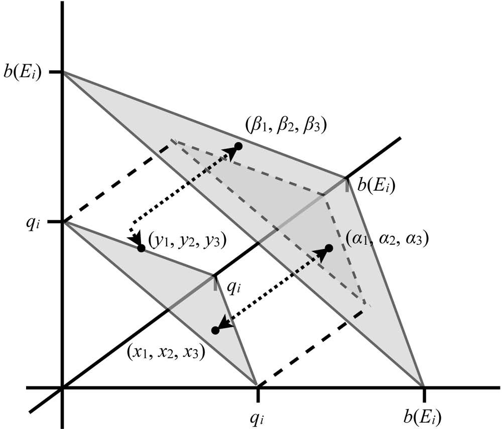
Admittedly, the statement of this norm is not so transparent as Jeffrey's, but it follows from the proof of theorem 5 that there is a natural geometric interpretation of the update rule that it describes. This is illustrated in figure 1. Consider the element  $E_{i}$ of the partition. And suppose that with respect to
 $E_{i}$, the agent's belief function at t is represented by a point that lies within the larger gray triangle (as
 $( \alpha _{1},\:\alpha _{2},\:\alpha _{3}) $ and
 $( \beta _{1},\:\beta _{2},\:\beta _{3}) $ do). Then our evidence imposes the constraint that her belief function at t′ assigns
 $q_{i}$ to
 $E_{i}$ and hence must be represented by a point that lies within the smaller gray triangle. As it turns out, the point that minimizes global expected inaccuracy relative to this constraint is the point within the smaller gray triangle that lies closest to the point representing the original belief function, when that distance is measured by the Euclidean metric. Our statement of the updating rule above provides an analytic description of this point. Indeed, there are two cases: if the projection of the original belief function lies within the smaller gray triangle, then this projection already represents the belief function demanded by the updating rule (as is the case for
 $( \alpha _{1},\:\alpha _{2},\:\alpha _{3}) $ and its projection
 $( x_{1},\: x_{2},\: x_{3}) $ in fig. 1). If it does not, the updated belief function is represented by the point on the smaller gray triangle that lies closest to that projection (as is the case for
 $( \beta _{1},\:\beta _{2},\:\beta _{3}) $ and
 $( y_{1},\: y_{2},\: y_{3}) $ in fig. 1).
Figure 1.

Having seen the updating rule sanctioned by the relevant version of Accuracy in Jeffrey cases, a number of its features deserve our attention. In section 7.1, we give an example to show that Jeffrey's rule results in belief functions with greater expected global inaccuracy than those given by our alternative rule. In section 7.2, we note that, as with Jeffrey's rule, the order in which compatible side constraints are imposed affects the posterior probability given by our rule: that is, our rule is noncommutative. We appeal to an insight of Marc Lange to show that this raises no objection. In section 7.3, we observe that Conditionalization is not a particular case of our rule, and we explain why this is as it should be. In section 7.4, we note that, unlike Jeffrey's rule, our rule can be used to raise probabilities from zero. And, in section 7.5, we reconsider the way in which the objective or ‘quasi-logical’ content of the diachronic versions of our Accuracy norm combine with the subjective or ‘extralogical’ constraints C that are fed into it, and we thereby address a possible objection concerning the rigidity of conditional probabilities.
7.1. The Expected Global Inaccuracy of Jeffrey's Rule
Suppose I see a person in the distance, and I know that it is one of three people: in  $w_{1}$, it is Paul, who is male and has blond hair; in
 $w_{2}$, it is Jeff, who is male and has black hair; in
 $w_{3}$, it is Taj, who is female and has black hair. Suppose further that I know that the actual world is a member of
 $W=\{ w_{1},\: w_{2},\: w_{3}\} $. At time t, I have the following belief function:

And between t and t′, I have an experience that does not rule out any possible worlds but that imposes the following side constraints on my beliefs:

Then Jeffrey's rule leads to the following values for  $b_{t^{\prime }}$:

If we let  $G( \{ w,\: b\} ) =\vert \vert w-b_{\mathrm{glo}\,}\vert \vert ^{2}$, then

However, our rule leads to the following values for  $b_{t^{\prime }}$:Footnote 13

So

Thus, the expected global inaccuracy of the feasible belief function that results from Alternative Jeffrey Conditionalization is lower than the expected global inaccuracy of the feasible belief function that results from Jeffrey Conditionalization.Footnote 14
7.2. Noncommutativity and the Sameness of Experience
We can extend the example of the previous section to show that, like Jeffrey Conditionalization, our rule is fundamentally noncommutative: that is, given a series of side constraints, and given successive applications of the rule that respect each of these side constraints in turn, the order in which the side constraints are imposed affects the final result; what is more, this remains true even when the side constraints are compatible in the sense that there are probability functions that satisfy them all at once.
One immediate—and, as we think, valid—reply to this is, so what? If we have to balance some of our pretheoretical intuitions against a (hopefully) carefully crafted argument based on mathematical proof and established normative principles, it should be obvious which way to go. But let us examine the issue more closely and independently of such considerations.
In the previous section, we began with a belief function  $b_{t}$ and some side constraints on
 $b_{t^{\prime }}$. Then we compared the effect of updating to a belief function that satisfies these side constraints using our rule and using Jeffrey's. We begin the following consideration by stating a new set of side constraints:

It is clear that this is compatible with the side constraints in the previous section, for there is at least one probability function that satisfies both.Footnote 15 However, as the calculations below show, if one begins with  $b_{t}$ and then imposes the side constraint from the previous section and then the side constraint from this section, our rule demands a belief function that differs from the belief function it demands if the order is reversed:Footnote 16
1. First, impose
$b_{t^{\prime }}( \{ w_{1},\: w_{2}\} ) =1/ 2$:
Second, impose$b_{t^{\prime \prime }}( \{ w_{2},\: w_{3}\} ) =3/ 4$:
2. First, impose
$b_{t^{\prime }}( \{ w_{2},\: w_{3}\} ) =3/ 4$:
Second, impose$b_{t^{\prime \prime }}( \{ w_{1},\: w_{2}\} ) =1/ 2$:



Some have taken the analogous result in the case of Jeffrey Conditionalization to be a flaw that is fatal for that rule (van Fraassen Reference van Fraassen1989; Döring Reference Döring1999). The objection, which is a reductio, is based on the following premise, which is made plausible in some toy story: in the situations described in 1 and 2 above, the first side constraint in 1 and the second side constraint in 2 have to be consequences of the same sensory experience; likewise, the second side constraint in 1 and the first side constraint in 2 have to be consequences of the same sensory experience. From this it follows that, on our rule or on Jeffrey's, one could obtain different belief functions simply by having the same sensory experiences but in a different order. This, the objector claims, is counterintuitive, and the reductio is complete.
The correct reply to this objection is already present in Field (Reference Field1978) and Skyrms (Reference Skyrms1986, 197), but it is only stated explicitly by Marc Lange (Reference Lange2000; see also Wagner [Reference Wagner2002], 274–75, for a similar point). It is simply that reversing the order of side constraints does not necessarily correspond to reversing sensory experiences. Being subject to the same side constraints due to what has been going on qualitatively in one's sensory organs is not sufficient for having the same sensory experiences; in order to individuate sensory experiences, one also has to take into account the effect that the side constraints have on one's prior belief function and indeed the prior belief function on which they have that effect.
Thus, rather than being a flaw in our rule and in Jeffrey's, we should expect commutativity to fail for updating rules that apply to the cases Jeffrey considers. After all, on the view just explained, a particular side constraint corresponds to different sensory experiences if it is imposed on different prior belief functions. And we should not be surprised to find different sequences of sensory experience to give rise to different posterior belief functions.
7.3. Why Conditionalization Is Not a Special Case
Conditionalization is the special case of Jeffrey Conditionalization obtained by taking the partition  $\{ E_{1}=E,\: E_{2}=\neg E\} $ and letting
 $q_{1}=1$ and
 $q_{2}=0$. One might expect the same to hold of our rule, but this is not the case.
The reason is simple. There are two different sorts of constraint that new evidence can impose on an agent's epistemic state: it can impose side constraints on the belief function that the agent should adopt in the light of the evidence, and it can restrict the set of worlds that are epistemically possible for the agent in the light of the evidence. Jeffrey Conditionalization is usually supposed to cover the former sort of situations; Conditionalization covers situations in which the latter sort of constraint is imposed. In the context of our theory, one deals in the former case with minimizing sums of the form

where b is the (given) current belief function and where b′ is unspecified except for the demand to satisfy the side constraints. In the latter case, however, one intends to minimize sums of the form

in which b is again the (given) current belief function, b′ is left completely unspecified, and where the sum is taken only over the worlds in E. If one tried to emulate conditionalization by the Jeffrey-type requirement that  $b^{\prime }( E) =1$, then any permissible choice of b′ would indeed assign 0 to
 $\neg E$, but this would still not necessarily be so for b; hence, in the emulation of conditionalization, inaccuracies with respect to worlds outside of E might still play a role, in contrast with the proper conditionalization case.
Thus, it is entirely appropriate that Conditionalization is not a special case of our rule. Learning a proposition with certainty is not the limiting case as the side constraints  $q_{1}$ and
 $q_{2}$ on the partition
 $\{ E_{1}=E,\: E_{2}=\neg E\} $ tend to 1 and 0, respectively, for as these values tend to zero, the set of epistemically possible worlds remains constantly W. Thus, the correct updating rule in the situations normally assumed to be covered by Jeffrey Conditionalization should not necessarily tend to Conditionalization in the limit.
7.4. Raising Credences from Zero
It is a well-known feature of Jeffrey Conditionalization that it cannot raise the probability of a proposition from zero. Thus, if this is the correct updating rule, we must forever assign zero to each proposition to which we currently assign zero. This, it has sometimes been argued, is too strong. It rules out the possibility of rationally coming to believe something that one once considered certainly false, yet this is surely possible.
It is a virtue of our rule that it does not have this consequence. Indeed, given a proposition A and a belief function  $b_{t}$ such that
 $b_{t}( A) =0$, our rule applies even if the evidence an agent obtains results in the following side constraint on her belief function at t′:
 $b_{t^{\prime }}( A) =p> 0$ and
 $b_{t\prime }( \neg A) =1-p$. Jeffrey Conditionalization is not even defined in this case.
7.5. The Logic versus the Art of Judgment
In the light of the previous findings, let us reconsider one more time the norm on which the justification of our new rule of update is based:Footnote 17
Accuracy (Diachronic expected global). At time t′, an agent ought to have a belief function that satisfies constraints C and is minimal among belief functions thus constrained with respect to expected global inaccuracy by the lights of your belief function at time t, relative to a legitimate global inaccuracy measure and over the set of worlds that are epistemically possible for her at time t′ given the constraints C.
The norm combines two kinds of constraints: (i) one ought to minimize one's expected global inaccuracy given certain parameters; (ii) the latter parameters are characterized in the way that they ought to satisfy C. What is the philosophical status of these constraints?
We regard ii as being given subjectively or ‘extralogically’. Within our theory, there is no room for justifying why C is such and such in a concrete application of Accuracy (Diachronic expected global) by a real-world agent. However, within the range of possibilities left open by C, it is a matter of epistemic rationality—a matter of getting as close to the truth as possible—to obey i. In this sense, i is an objective or ‘quasi-logical’ constraint but one that is conditional on the antecedently specified C condition. If C is, for example, such that the one and only belief function  $b_{t^{\prime }}$ can satisfy it, then minimizing one's expected global inaccuracy in the range of possibilities as determined by C will be a trivial affair, and so be it according to our proposal.
As explained in the previous sections, conditionalization results from an application of Accuracy (Diachronic expected global) with an antecedent constraint C of the form ‘restrict your set of epistemically possible worlds at t′ to the set E’. In contrast, the new update rule that we have focused on in this last part of our article is due to an application of Accuracy (Diachronic expected global) with an antecedent constraint C of the form ‘change your degrees of belief in a way such that for all i,  $E_{i}$ is believed at t′ with degree q
i
'. While these applications of Accuracy (Diachronic expected global) are clearly of broad interest, nothing prevents us from demanding other extralogical constraints C to be satisfied at t′ and consequently to search for rules of update that would minimize expected global inaccuracy in such circumstances.
For instance, one might be interested in a constraint C of the form ‘change your degrees of belief in a way such that for all i,  $E_{i}$ is believed at t′ with degree
 $q_{i}$, and furthermore Rigidity is satisfied; that is,
 $b_{t^{\prime }}( A\vert E_{i}) =b_{t}( A\vert E_{i}) $ for all propositions
 $A\subseteq W$’. As noted before, Jeffrey's rule is the unique updating rule that leads to belief functions that satisfy this type of constraint. The fact that our rule of update differs from Jeffrey's should not be taken to imply that ours is ‘logically valid’ and Jeffrey's is not (or vice versa) but rather that the two rules are the objectively justified outcomes of solving one and the same epistemic problem—to get as close to the truth as possible—but in two different problem spaces.
This general line of reasoning could only be undermined by an argument that would show that some constraints C are ‘more objective’ or ‘more logical’ or ‘more rational’ than others. While we do not think that this can be ruled out completely, our theory does not offer any resources to put forward any plausible argument of that sort, and at least with respect to the question of whether to demand Rigidity or not, it is very hard to see that any such argument could be given at all. Indeed, we agree with Bradley (Reference Bradley2005) that sometimes Rigidity ought not to be demanded, in particular, when changes in belief give inferential grounds for changes in conditional belief. In principle, very much the same applies to the constraint that leads to simple conditionalization, however with one difference: in our theory, conditionalization is the objective consequence of the extralogical constraint ‘restrict your set of epistemically possible worlds at t′ to the set E’ in which Rigidity with respect to the partition  $\{ E,\:\neg E\} $ is not contained. It is only once the minimization problem is solved that Rigidity is seen to hold for the resulting solution strategy, that is, conditionalization. In this sense, the rigidity of plain conditionalization is ‘more objective’ than the rigidity of Jeffrey conditionalization. But of course even standard conditionalization might have to go if some other extralogical constraint C is chosen, for whatever reason.
8. Some Open Questions
Obviously, our defense of Bayesianism in terms of minimizing expected inaccuracy leaves a lot of problems untouched. It is only fair to summarize the main open questions in the final section of this article, posed as a challenge to future expansions of the theory:
• We asked this in the final section of this article's prequel, but it is relevant again: How can the approach be extended to the case of an infinite set of worlds, in particular, to the case of nondenumerably many possible worlds? What role does countable additivity play in such extensions?
• Is it possible to develop a similar theory for primitive conditional belief functions, such as Popper measures, which allow for conditionalization on zero sets? Alternatively, what does a corresponding approach to nonstandard probability measures look like?
• Is it possible to adapt this style of argument—by changing one of our presuppositions in some way—in order to justify other accounts of belief and belief update as well (e.g., the Dempster-Shafer approach)?
• Given a different sort of constraint imposed by a piece of evidence, which updating rule does Accuracy (Diachronic expected global) prescribe? For instance:
• Suppose an agent's evidence leads her to impose the following side constraints on
$b_{t^{\prime }}$: $b_{t^{\prime }}( A) =p$ and $b_{t^{\prime }}( B) =q$, where $A\cap B\neq \emptyset $. What is the prescribed rule of update?• Or suppose that
$\{ E_{1},\: E_{2},\: E_{3}\} $ is a partition on W and the agent's evidence leads her to impose the following side constraints on $b_{t^{\prime }}$: $b_{t^{\prime }}( E_{1}) =kb_{t^{\prime }}( E_{2}) $, where $k\in \mathstrut{\Bbb R} ^{+}_{0}$. What is the prescribed rule of update in this case? (This is closely related to van Fraassen's [Reference van Fraassen1981] well-known Judy Benjamin problem.)Footnote 18
• It is easy to show that Accuracy (Diachronic expected local) is not always satisfiable given constraints C on the future belief function as used in Jeffrey Conditionalization (see appendix). Which belief functions at time t and which choices of epistemically possible worlds yield satisfiable instances of Accuracy (Diachronic expected local) for such C? In cases in which Accuracy (Diachronic expected local) cannot be satisfied, what do the belief functions look like that approximate Accuracy (Diachronic expected local) in the ‘best possible’ way, and how do these belief functions formally relate to the updating rule that we derived from Accuracy (Diachronic expected global)?


Answering these questions satisfactorily should not only lead to interesting extensions of our theory, but it should also help minimizing the inaccuracies of the theory as it stands.
Appendix: Proofs of Theorems 2–5 and Accuracy (Diachronic Expected Local) Again
Proofs of Theorems 2–4
The proof of each of our theorems depends on the following lemma.
Lemma 6. Suppose  $I( A,\: w,\: x) =\lambda ( \chi _{A}( w) -x) ^{2}$. Suppose W is finite, b and
 $b^{\prime }$ are belief functions,
 $A,\: E\subseteq W$, and
 $\sum_{w\in E}b( w) \neq 0$. Then the following two propositions are equivalent:
i) For all
$A\subseteq W$ and all $x\in \mathstrut{\Bbb R} ^{+}_{0}$,
ii) For all
$A\subseteq W$,


Proof. By definition,

So,

Therefore,

if and only if

Since  $\sum_{w\in E}b( \{ w\} ) I( A,\: w,\: x) $ is a positive quadratic in the variable x, this extremum is a minimum, as required. QED
Proof of Theorem 2
Suppose b is a belief function and  $E\subseteq W$, with
 $\sum_{w\in E}b( \{ w\} ) \neq 0$. Then, by lemma 6, it suffices to show that

if and only if b is a probability function on the power set of W and  $b( \{ w\} ) =0$ for
 $w\not\in E$.
First, we prove the ‘if’ direction. We begin by showing that, if b is a probability measure and  $b( \{ w\} ) =0$ for
 $w\not\in E$, then for all
 $A\subseteq W$,

If b is a probability measure and  $b( \{ w\} ) =0$ for
 $w\not\in E$, then

So,

as required.
Second, we prove the ‘only if’ direction. That is, we show that, if b is a belief function and, for all  $A\subseteq W$,

then, as required, it follows that b satisfies 1–3 below, the Kolmogorov axioms:
1. If
$A\subseteq W$, then $b( A) \geq 0$. This is obvious, since $b\thinspace{:}\thinspace P( W) \rightarrow \mathstrut{\Bbb R} ^{+}_{0}$.2. Function
$b( \emptyset ) =0$ and $b( W) =1$:
and3. If
$A,\: B\subseteq W$ are disjoint, then $b( A\cup B) =b( A) +b( B) $. If $A,\: B\subseteq W$, then
since$( A\cup B) \cap E=( A\cap E) \cup ( B\cap E) $.


Furthermore, if  $w\not\in E$, then obviously
 $b( \{ w\} ) =0$. QED
Proof of Theorem 3
Suppose  $b_{t}$ is a probability function,
 $I( A,\: w,\: x) =\lambda ( \chi _{A}( w) -x) ^{2}$, and
 $E\subseteq W$ with
 $b_{t}( E) \neq 0$. Then it follows immediately from lemma 6 that, for all
 $A\subseteq W$,

is minimal, if and only if

as required. QED
Proof of Theorem 4
Suppose  $I( A,\: w,\: x) =\lambda ( \chi _{A}( w) -x) ^{2}$. Then, in lemma 6, let
 $b( \{ w\} ) =1$ for all
 $w\in W$. Then

is minimal, if and only if

as required. QED
Proof of Theorem 5
Suppose  $\{ E_{1},\:\ldots ,\: E_{m}\} $ is a partition of W. Suppose
 $0\leq q_{1},\:\ldots ,\: q_{m}$ and
 $q_{1}+\ldots +q_{m}=1$. Suppose
 $G( w,\: b) =\vert \vert w-b_{\mathrm{glo}\,}\vert \vert ^{2}$, and suppose that
 $b_{t}$ is a probability function: let
 $\alpha _{j}=b_{t}( \{ w_{j}\} ) $ for
 $j=1,\:\ldots ,\: n$. We wish to find the probability function
 $b_{t^{\prime }}$ represented by the vector
 $( x^{*}_{1},\:\ldots ,\: x^{*}_{n}) $ such that the function

is minimal at  $( x^{*}_{1},\:\ldots ,\: x^{*}_{n}) $ relative to the following side constraints:

We say that a vector  $( x_{1},\:\ldots ,\: x_{n}) $ is feasible if it satisfies these constraints.
Now, we begin by reformulating the function we wish to minimize as follows:

Now, it is clear that

is minimal among the feasible vectors, if and only if

is minimal among the feasible vectors. Thus,  $b_{t^{\prime }}$ is minimal, just in case it is represented by the closest feasible vector
 $( x^{*}_{1},\:\ldots ,\: x^{*}_{n}) $ to
 $( \alpha _{1},\:\ldots ,\:\alpha _{n}) $ as measured by the Euclidean metric. But how do we find this closest feasible vector?
It is clear that

is minimal among the feasible vectors if and only if, for each  $i=1,\:\ldots ,\: m$, if
 $E_{i}=\{ w_{l_{1}},\:\ldots ,\: w_{l_{k}}\} $, then

is minimal among those vectors  $( x_{l_{1}},\:\ldots ,\: x_{l_{k}}) $ for which
 $x_{l_{1}}+\ldots +x_{l_{k}}=q_{i}$ and
 $x_{l_{j}}\geq 0$ for all
 $j=1,\:\ldots ,\: k$. Thus, it suffices to solve the minimization problem separately for each element
 $E_{i}$ of the partition.
We now give two different ways of showing that the vector given by Alternative Jeffrey Conditionalization solves each of these separate minimization problems. The first is our original proof and proceeds via the theory of convex quadratic programming and the Karush-Kuhn-Tucker (KKT) conditions that are central to that theory. The second is a purely geometric argument that we owe to Kenny Easwaran. We include both here since they exhibit quite different virtues. On the one hand, Easwaran's argument is simpler and requires less mathematical apparatus, but it is not clear how to generalize his approach so that it applies in updating situations that arise when different sorts of constraints are imposed on  $b_{t^{\prime }}$. On the other hand, our original argument from KKT conditions requires more powerful machinery, but it has the advantage of being fully general.
In what follows, we assume, without loss of generality, that  $E_{i}=\{ w_{1},\:\ldots ,\: w_{k}\} $. This will avoid unnecessarily complicated subscripts. First, the argument from KKT conditions. The mathematical theorem we require is as follows:Footnote 19
Theorem 7 (KKT conditions). Suppose  $f,\: g_{1},\:\ldots ,\: g_{m},h_{1},\:\ldots ,\: h_{n}\thinspace{:}\thinspace \mathstrut{\Bbb R} ^{k}\rightarrow \mathstrut{\Bbb R} $ are smooth functions. Consider the following minimization problem. Minimize
 $f( x_{1},\:\ldots ,\: x_{k}) $ relative to the following constraints:

If is a (nonsingular) solution to this minimization problem, then there exist  $\mu _{1},\:\ldots ,\:\mu _{m}$,
 $\lambda _{1},\:\ldots ,\:\lambda _{n}\in \mathstrut{\Bbb R} $ such that

If, furthermore, f and g are convex functions, then the existence of  $\mu _{1},\:\ldots ,\:\mu _{m}$,
 $\lambda _{1},\:\ldots ,\:\lambda _{n}\in \mathstrut{\Bbb R} $ is sufficient for a solution to the minimization problem. If f is strictly convex, then their existence is sufficient for a unique solution.
Stated in the form used in the theorem, here is the problem we must solve. Minimize

relative to the following constraints:

Thus, since  $f_{i}$,
 $g_{1},\:\ldots ,\: g_{k}$, and h are smooth functions and since
 $f_{i}$ is strictly convex, it is sufficient for
 $( x^{*}_{1},\:\ldots ,\: x^{*}_{k}) $ to be a unique solution to this minimization problem that
 $( x^{*}_{1},\:\ldots ,\: x^{*}_{k}) $ satisfies the constraints and there exist
 $\mu _{1},\:\ldots ,\:\mu _{k},\:\lambda \in \mathstrut{\Bbb R} $ such that, for all
 $j=1,\:\ldots ,\: k$,
i) Value
$\mu _{j}\geq 0.$ii) Value
$\mu _{j}x^{*}_{j}=0$.iii) And
$2x^{*}_{j}-2\alpha _{j}-\mu _{j}+\lambda =0$.



Now, define  $d_{i}$ as in Alternative Jeffrey Conditionalization, and let

In order to prove theorem 5, it suffices to show that  $( x^{*}_{1},\:\ldots ,\: x^{*}_{k}) $ thus defined satisfies the constraints and that there are
 $\mu _{1},\:\ldots ,\:\mu _{k},\:\lambda \in \mathstrut{\Bbb R} $ that satisfy i–iii. It is straightforward to see that
 $( x^{*}_{1},\:\ldots ,\: x^{*}_{k}) $ satisfies the constraints. Now define

and

It is straightforward to see that i–iii then hold. This completes our first proof of theorem 5.
We turn now to Kenny Easwaran's geometric proof. First, we note that, since the set of feasible vectors is closed and bounded and since the Euclidean distance from  $( \alpha _{1},\:\ldots ,\:\alpha _{k}) $ to
 $( x_{1},\:\ldots ,\: x_{k}) $ is a continuous function of
 $( x_{1},\:\ldots ,\: x_{k}) $, there is at least one feasible vector
 $( x^{*}_{1},\:\ldots ,\: x^{*}_{k}) $ such that the Euclidean distance from
 $( \alpha _{1},\:\ldots ,\:\alpha _{k}) $ to that vector is minimal. Next, we use the following lemma to identify the unique such feasible vector.
Lemma 8. Suppose  $( x_{1},\:\ldots ,\: x_{k}) $ is feasible. Then, if
 $x_{b}> 0$ and
 $x_{a}-\alpha _{a}< x_{b}-\alpha _{b}$, then the distance from
 $( \alpha _{1},\:\ldots ,\:\alpha _{k}) $ to
 $( x_{1},\:\ldots ,\: x_{k}) $ is not minimal among the feasible vectors.
Proof. Suppose  $( x_{1},\:\ldots ,\: x_{a},\:\ldots ,\: x_{b},\:\ldots ,\: x_{k}) $ is feasible, and suppose that
 $x_{b}> 0$ and
 $x_{a}-\alpha _{a}< x_{b}-\alpha _{b}$. Then let ε be a positive real number such that

Then  $( x_{1},\:\ldots ,\: x_{a}+\varepsilon ,\:\ldots ,\: x_{b}-\varepsilon ,\:\ldots ,\: x_{k}) $ is also feasible. Moreover, a quick calculation shows that it is closer to
 $( \alpha _{1},\:\ldots ,\:\alpha _{k}) $ than is
 $( x_{1},\:\ldots ,\: x_{a},\:\ldots ,\: x_{b},\:\ldots ,\: x_{k}) $. This completes the proof of the lemma.
With this in hand, we can identify the unique vector whose distance from  $( \alpha _{1},\:\ldots ,\:\alpha _{k}) $ is minimal. We require two corollaries to the lemma.
First corollary. Suppose  $( x^{*}_{1},\:\ldots ,\: x^{*}_{k}) $ is minimal; then there is a real number
 $d_{i}$ such that, if
 $x^{*}_{a}> 0$, then
 $x^{*}_{a}=\alpha _{a}+d_{i}$.
Proof. Suppose  $x^{*}_{a},\: x^{*}_{b}> 0$. Then, by the lemma, it must be that
 $x_{a}-\alpha _{a}=x_{b}-\alpha _{b}$. Thus, there is
 $d_{i}=x_{a}-\alpha _{a}=x_{b}-\alpha _{b}$, as required.
Second corollary. Suppose  $( x^{*}_{1},\:\ldots ,\: x^{*}_{k}) $ is minimal, and suppose that, whenever
 $x^{*}_{a}> 0$, we have
 $x^{*}_{a}=\alpha _{a}+d_{i}$; then, whenever
 $\alpha _{a}+d_{i}> 0$, we have
 $x^{*}_{a}=\alpha _{a}+d_{i}$.
Proof. Suppose not. That is, suppose  $\alpha _{a}+d_{i}> 0$ and
 $x^{*}_{a}\neq \alpha _{a}+d_{i}$. Then, by the previous corollary,
 $x^{*}_{a}=0$. Now suppose
 $x_{b}> 0$. Then

Thus, by the lemma,  $( x^{*}_{1},\:\ldots ,\: x^{*}_{k}) $ is not minimal. This contradicts the assumption, as required.
From these two corollaries to the lemma, we have that, if  $( x^{*}_{1},\:\ldots ,\: x^{*}_{k}) $ is minimal, there is
 $d_{i}$ such that, for all
 $j=1,\:\ldots ,\: k$,
a) If
$\alpha _{j}+d_{i}> 0$, then $x^{*}_{j}=\alpha _{j}+d_{i}$.b) If
$\alpha _{j}+d_{i}\leq 0$, then $x^{*}_{j}=0$.c) And
$\sum_{j=1}^{k}x^{*}_{j}=q_{i}$.


That is, the vector to which Alternative Jeffrey Conditionalization gives rise is the closest vector to  $( \alpha _{1},\:\ldots ,\:\alpha _{k}) $, as required. This completes the second proof of theorem 5, due to Kenny Easwaran. QED
Accuracy (Diachronic Expected Local) Cannot Always Be Satisfied in Jeffrey Situations
In proofs of theorems 2 and 3, we derived Probabilism and Conditionalization from the local synchronic and diachronic versions of Accuracy, respectively. But we derived our alternative to Jeffrey's rule from the global diachronic version of Accuracy (along with Probabilism, which is guaranteed by Accuracy (Synchronic expected local)). Above, we mentioned why this is: the local version cannot always be satisfied in the situations to which Jeffrey Conditionalization claims to apply. In this section, we prove this.
First, recall that Accuracy (Diachronic expected local) entails Accuracy (Diachronic expected global). That is, any belief function that satisfies the former satisfies the latter. Also, we know which belief function satisfies the latter, in virtue of theorem 5, proved above. Thus, it will suffice to describe a Jeffrey situation in which the belief function that satisfies Accuracy (Diachronic expected global) does not satisfy Accuracy (Diachronic expected local).
Consider again the example of section 7.1. That is,  $W=\{ w_{1},\: w_{2},\: w_{3}\} $ and

We then impose the following constraint:  $b_{t}( \{ w_{1},\: w_{2}\} ) =1/ 2$. Then our updating rule gives

Let  $I( A,\: w,\: x) =( \chi _{A}( w) -x) ^{2}$, and consider the expected local inaccuracy of the degree of credence
 $b^{A}_{t^{\prime }}( \{ w_{1}\} ) $ in the singleton proposition
 $\{ w_{1}\} $ by the lights of
 $b_{t}$, relative to I and over all possible worlds in W:

Now consider the following belief function:

Then

Thus,

As noted above, this suffices to show that Accuracy (Diachronic expected local) cannot be satisfied in all Jeffrey situations. QED