
1. Introduction
An aquifer is a porous rock or deposit saturated with water. In most geological settings, groundwater is in mechanical contact with the atmosphere through the pores of the overlying soil. The aquifer is then said to be ‘unconfined’, and the free surface of the groundwater body is called the ‘water table’ (Ingebritsen & Sanford Reference Ingebritsen and Sanford1999). Unconfined aquifers are recharged by precipitations. Rainwater infiltrates into the soil, and percolates through the unsaturated zone until it reaches the water table (Kirchner, Feng & Neal Reference Kirchner, Feng and Neal2000). This groundwater then flows through the aquifer, and eventually emerges into streams to form surface runoff.
The time rainfall needs to travel through the aquifer controls the chemical weathering of the porous rock, and the propagation of dissolved contaminants towards the drainage network (Kirchner et al. Reference Kirchner, Feng and Neal2000; Godsey et al. Reference Godsey2010; Maher Reference Maher2010; Rempe & Dietrich Reference Rempe and Dietrich2014). As it travels through the aquifer, a parcel of groundwater gradually spreads under the combined action of three processes: (1) molecular diffusion, which results from thermal fluctuations at the molecular scale; (2) hydrodynamic dispersion, which results from velocity fluctuations at the pore scale; and (3) advection by the average velocity of groundwater, which varies at the scale of the aquifer (Saffman Reference Saffman1959; De Marsily Reference De Marsily1986; Charlaix, Hulin & Plona Reference Charlaix, Hulin and Plona1987). The travel time of water through the aquifer results from the combination of these processes, which, in its turn, depends on the geometry and scale of the groundwater flow (Le Borgne et al. Reference Le Borgne, de Dreuzy, Davy and Bour2007; Dentz et al. Reference Dentz, Le Borgne, Englert and Bijeljic2011).
Field measurements, based on isotopic ratios or conservative tracers, reveal that the mean travel time of water typically ranges from a few months to millennia (Gleeson et al. Reference Gleeson, Befus, Jasechko, Luijendijk and Cardenas2016; Cartwright et al. Reference Cartwright, Cendón, Currell and Meredith2017). Over such a long time, runoff balances recharge, and one may consider that the flow is in steady state (Cardenas Reference Cardenas2007).
In nature, most aquifers extend much further horizontally than vertically, which makes the groundwater flow amenable to the shallow-water approximation. Combined with Darcy's law (Darcy Reference Darcy1856), the latter provides a simplified description of the flow, in the form of the Dupuit–Boussinesq equation (Dupuit Reference Dupuit1863; Boussinesq Reference Boussinesq1903). This theory, which neglects the vertical component of the flow, consistently accounts for the fluctuations of the water table caused by intermittent rainfall (Brutsaert & Nieber Reference Brutsaert and Nieber1977; Troch et al. Reference Troch2013; Guérin, Devauchelle & Lajeunesse Reference Guérin, Devauchelle and Lajeunesse2014; Guérin et al. Reference Guérin, Devauchelle, Robert, Kitou, Dessert, Quiquerez, Allemand and Lajeunesse2019). When averaged over a sufficiently long time, however, these fluctuations vanish, and the average water table conforms to the steady-state Dupuit–Boussinesq equation (Guérin et al. Reference Guérin, Devauchelle, Robert, Kitou, Dessert, Quiquerez, Allemand and Lajeunesse2019). On average, one then finds that the water table mirrors the land's surface, with summits far from rivers, and valleys that line the drainage network (Petroff et al. Reference Petroff, Devauchelle, Abrams, Lobkovsky, Kudrolli and Rothman2011; Devauchelle et al. Reference Devauchelle, Petroff, Seybold and Rothman2012).
In reality, however, the stream that drains a catchment often lies above the base of the aquifer. Groundwater must therefore rise to reach the outlet (Lehr Reference Lehr1963), and the vertical component of the resulting flow violates the Dupuit–Boussinesq approximation (Powers, Kirkham & Snowden Reference Powers, Kirkham and Snowden1967; Read Reference Read1993; Haria & Shand Reference Haria and Shand2004; Bresciani, Davy & de Dreuzy Reference Bresciani, Davy and de Dreuzy2014). In this configuration, the velocity potential that drives the flow obeys the Laplace equation, the solution of which crucially depends on the boundary conditions (Polubarinova-Kochina Reference Polubarinova-Kochina1962). One often assumes that the flow is bounded by a horizontal impervious layer at its base, while impervious boundaries represent the water divides on its sides (Toth Reference Toth1963). The groundwater pressure must also match the atmospheric one along the water table. This last boundary condition, however, is more challenging than the others: the position of the water table is not specified a priori, and needs to be solved for.
Turning the similarity between the water table and the land surface into a boundary condition, Toth (Reference Toth1963) assumed that the water-table elevation is proportional to that of the land surface, and set the groundwater pressure accordingly. Mathematically, this is a Dirichlet condition: the value of the potential is specified at the boundary (Farlow Reference Farlow1993). The resulting flow is then entirely determined by the land's topography: groundwater sinks below hills, and rises towards valleys (Toth Reference Toth1963; Cardenas Reference Cardenas2007).
This hypothesis, although leading to realistic-looking flows, is nevertheless unjustified. In reality, the water table freely adjusts its shape to accommodate the rainfall input, and there is no reason to believe that, in doing so, it follows the shape of the land's surface exactly. Instead of specifying the water table a priori, one must solve the flow equations to get it (Polubarinova-Kochina Reference Polubarinova-Kochina1962), and this free-boundary problem requires not one, but two boundary conditions at the water table. In addition to setting the groundwater pressure, one must also account for the flux of rainwater that reaches the water table (Powers et al. Reference Powers, Kirkham and Snowden1967). Mathematically, this is a Stefan problem: the values of both the potential and its derivative are specified at the boundary, the position of which must be solved for (Rubinstein Reference Rubinstein2000). One thus needs to solve the Laplace equation inside a domain that is a priori unknown.
How does the aquifer's geometry influence such a flow? Is it possible to infer this geometry based on the residence time of water in the aquifer? Inspired by Guérin et al. (Reference Guérin, Devauchelle and Lajeunesse2014), we address these questions in a laboratory experiment. We begin with the description of the experimental set-up (§ 2). We then focus on the steady-state regime (§ 3). We derive an analytical solution for this regime and compare it to experimental streamlines (§ 4). We then compute the travel time of water, and show how the aquifer's aspect ratio affects it (§ 5). Finally, we estimate the magnitude of hydrodynamic dispersion in our experiment (§ 6).
2. Laboratory aquifer
2.1. Set-up
At its simplest, an unconfined aquifer consists of a homogeneous porous medium, the upper surface of which is in contact with the atmosphere. Inspired by Guérin et al. (Reference Guérin, Devauchelle and Lajeunesse2014), we reproduce this configuration in a narrow tank formed by two vertical Plexiglas® plates ( $90\ \mathrm {cm} \times 92\ \mathrm {cm}$), separated by a gap of width
 $W = 5\ \mathrm {cm}$ (figure 1). This tank is filled with glass beads of size either
 $1$ or
 $3\ \textrm {mm}$, which form an artificial aquifer bounded by an impermeable bottom. An impervious vertical wall closes the left side of the tank, mimicking the drainage divide of a catchment. We generate an artificial rain with an array of
 $24$ capillary tubes evenly spaced above the tank. These tubes (diameter
 $1.2\ \mathrm {mm}$, length
 $50\ \mathrm {cm}$) uniformly distribute water over the aquifer's surface, with a standard deviation of approximately
 $3\,\%$.
Experimental set-up and notations. The aquifer is made of glass beads (shaded area) piled between two vertical glass plates (black solid lines) separated by a gap of width  $W = 5\ \mathrm {cm}$. Its length and depth are
 $L=90$ cm and
 $H=62\ \mathrm {cm}$, respectively. A series of
 $24$ capillary tubes (diameter
 $1.2\ \mathrm {mm}$, length
 $50\ \mathrm {cm}$) placed above the tank simulate rainfall, by distributing water uniformly over the aquifer's surface.

We want to investigate the flow in a deep aquifer. To generate it, we bound the right-hand side of the aquifer with an impervious wall extending up to  $H=62\ \mathrm {cm}$ above the aquifer's bottom (figure 1). The remaining height (30 cm) is covered with a permeable vertical grid, which retains the glass beads, while allowing water to seep out. The aquifer's outlet thus lies high above its bottom. The corresponding aspect ratio is
 $H/L \approx 0.7$, where
 $L=90\ \mathrm {cm}$ is the length of the aquifer. The thinness of the set-up (
 $W/L\approx 0.05$), and its cross-wise invariance, ensure that the flow remains virtually two-dimensional.
When the grid that maintains the beads in the aquifer is directly in contact with the atmosphere, surface tension induces a pressure jump, which might affect the pressure field in the aquifer. To mitigate this inconvenience, we spread a soft plastic sheet over the outer side of the grid. This device maintains a thin film of water at atmospheric pressure over the grid surface, thus eliminating the effect of surface tension.
2.2. Method
Before each experimental run, we fill the aquifer with water until it overflows. After a few tens of minutes, the discharge at the aquifer's outlet has virtually vanished; the water table is then horizontal, and intersects the outlet. Starting from this initial condition, we switch on the artificial rain. An electromagnetic flowmeter (Kobold MIK 0.05–1 L min $^{-1}$, accuracy 2 %) measures the rainfall input,
 $Q_\textrm {in}$, from which we deduce the rainfall rate
 $R = Q_{in}/(LW)$. The latter then remains constant during the entire experiment.
As the rain falls on the aquifer's surface, it infiltrates into the porous medium, and seeps down until it reaches the water table, which deforms to accommodate this input. The asymmetry of the boundaries causes it to bend down towards the outlet (figure 1). As the resulting pressure field drives water towards the outlet, the aquifer's discharge increases, until it eventually reaches steady state, and balances the rainfall input ( $Q = RLW$).
A bucket collects the water that exits the aquifer. It lies on a scale which measures its weight every  $0.1\ \textrm {s}$ with a precision of
 $1\ \mathrm {mg}$. The water discharge
 $Q$ is the derivative of the bucket weight with respect to time. As water drips from the outlet, the discharge delivered to the bucket fluctuates around its average. As a result, the standard deviation of the steady-state discharge is approximately
 $0.3\ \textrm{mLs}^{-1}$, a value that is small compared with the range of discharge explored in our experiments (table 1).
Experimental parameters. The aquifer, made of 3 mm glass beads, has a hydraulic conductivity  $K = 9.1 \pm 0.3\ \mathrm {cm}\ \textrm {s}^{-1}$, and a permeability
 $k\approx 9.3\times 10^{-9}\ \textrm {m}^2$. The pore size is
 $d_p \sim \sqrt {k} \approx 0.1\ \textrm {mm}$.

Once the flow is steady, we inject small volumes of blue dye in the aquifer, and track their motion to trace the groundwater streamlines. We shall discuss the shape of these streamlines in § 3. Before we do so, however, we assess how the depth of our aquifer affects its response to rainfall, as compared to the shallow aquifer of Guérin et al. (Reference Guérin, Devauchelle and Lajeunesse2014).
2.3. Transient
Guérin et al. (Reference Guérin, Devauchelle and Lajeunesse2014) used an experiment similar to the present one, but for the position of the outlet which, in their set-up, lies right on the bottom of the aquifer ( $H=0$). In the following, we refer to this configuration as the ‘shallow aquifer’ because the water table remains close to the bottom.
For comparison with Guérin et al. (Reference Guérin, Devauchelle and Lajeunesse2014), we first use the same glass beads (diameter  $d_s=1\ \textrm {mm}$) and rainfall rate (
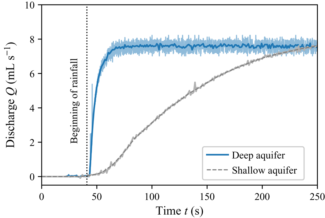
 $Q_{in} \approx 8\ \textrm {mL}\ \textrm {s}^{-1}$). Following the procedure of the previous section, we then record the time series of the discharge, often called hydrograph in this context. Less than five seconds after the beginning of rainfall, the discharge of our aquifer increases abruptly (figure 2). After a characteristic time of 10 to 15 seconds, it saturates, and reaches steady state. In the shallow aquifer of Guérin et al. (Reference Guérin, Devauchelle and Lajeunesse2014), the transient is surprisingly longer: it lasts several minutes (figure 2). The geometry of the flow also changes: the deformation of the water table is much smaller in the deep aquifer (a few millimetres) than in the shallow one (10 to 20 centimetres).
Discharge at the outlet of our deep experimental aquifer (blue line) and of a shallow one (black dashed line, Guérin Reference Guérin2015). Light colour: raw signal; dark colour: average over 10 successive data points. Vertical dotted line: beginning of rainfall. Both aquifers are  $5\ \textrm {cm}$ wide and
 $90\ \textrm {cm}$ long; they are made of the same 1 mm glass beads, and are submitted to similar rainfall inputs:
 $Q_{in} = 7.9\ \textrm {mL}~\textrm {s}^{-1}$ for the deep aquifer and
 $8.3\ \textrm {mL}\ \textrm {s}^{-1}$ for the shallow one.

The difference between our observations and those of Guérin et al. (Reference Guérin, Devauchelle and Lajeunesse2014) results from the boundary condition at the outlet. In the shallow aquifer, the flow is virtually parallel to the aquifer's bottom. According to the Dupuit–Boussinesq approximation, the discharge is then proportional to the water depth. The water level must therefore rise significantly before the flow can transport an amount of water that matches the input: it is this swelling that takes time. By contrast, the flow through a deep aquifer is free to develop a vertical component instantly, which allows water to flow through the whole aquifer right from the beginning of the rainfall event. The large volume of groundwater that an increase of pressure can mobilize thus allows the flow to respond instantly.
Unfortunately, the structure of this transient, two-dimensional flow is out of our reach in our experiment. In the next section, we focus instead on the steady state, which we visualize with dye. To this end, we substitute  $3\ \textrm {mm}$ glass beads for the
 $1\ \textrm {mm}$ ones, as they prove more convenient to track the propagation of the dye.
3. Streamlines
Once the flow is in steady state, we inject small parcels of blue dye into the aquifer, at different locations along its surface, and monitor their propagation. The dye consists of a mixture of deionized water ( $90\,\%$) and food colouring (Matfer,
 $10\,\%$). Its density (
 $997\ \mathrm {kg}\ \textrm {m}^{-3}$) is close to that of pure water; we therefore assume that it behaves as a passive tracer. To inject it in the aquifer, we use a set of six hypodermic needles, each of them connected to a syringe through a flexible pipe. The syringes are placed on a press (SPLab06, Schenchen Baoding), which allows us to simultaneously inject small volumes of blue dye (
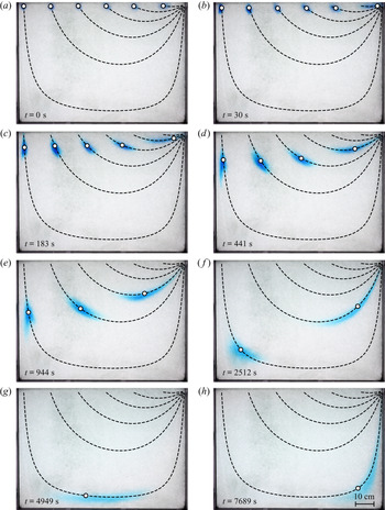
 $3\ \mathrm {mL}$) at six different locations, regularly spaced along the surface of the aquifer (figure 3).
Propagation of parcels of dye through the aquifer during run no. 1 (table 1, time indicated on each snapshot). Dye parcels are injected through the surface of the aquifer at distance  $\ell =87.3$,
 $72.7$,
 $57.6$,
 $42.5$,
 $27.4$, and
 $11.4\ \mathrm {cm}$ from the outlet. The aquifer, made of
 $3\ \mathrm {mm}$ glass beads, receives a rainfall input
 $Q_{in} = 6.3\ \mathrm {mL}\ \textrm {s}^{-1}$. Black dashed lines: streamlines after (4.11). White dots: position of the dye parcels after (5.1). Theory has no adjustable parameters.

Entrained by the flow, the parcels of dye then travel through the aquifer. A camera facing the set-up records an image of their position every 15 seconds (figure 3). A light panel, placed behind the aquifer, increases the contrast of the image.
We estimate the porosity of the aquifer by comparing the weights of a reference volume of beads successively filled with air and water. We find a porosity  $s\sim 0.4$, as expected for the random close packing of spheres (Andreotti, Forterre & Pouliquen Reference Andreotti, Forterre and Pouliquen2013). Following Lobkovsky et al. (Reference Lobkovsky, Jensen, Kudrolli and Rothman2004), we also measure the hydraulic conductivity of the aquifer using two communicating vessels connected by a Darcy column filled with
 $3\ \mathrm {mm}$ glass beads, and saturated with water. The release of a finite volume of water in one of the vessels induces a pressure gradient in the Darcy column, which drives a flow that tends to equilibrate the water levels in the vessels. The discharge then relaxes exponentially. The characteristic time of this relaxation depends on the hydraulic conductivity
 $K$ of the pack of beads. Using this method, we find
 $K = 9.1 \pm 0.3\ \mathrm {cm}\ \textrm {s}^{-1}$, from which we deduce the permeability of our aquifer,
 $k= \nu K/g \approx 9.3\times 10^{-9}\ \textrm {m}^2$, where
 $g$ is the acceleration of gravity, and
 $\nu$ the kinematic viscosity of water. Finally, we estimate the pore size from the permeability:
 $d_p \sim \sqrt {k} \approx 0.1\ \textrm {mm}$. This value is approximately 10 times smaller than the bead diameter, as observed in previous experiments (Souzy et al. Reference Souzy, Lhuissier, Méheust, Le Borgne and Metzger2020).
In total, we performed five experimental runs, varying the rainfall input between  $5$ and
 $16.7\ \textrm {mL}\ \textrm {s}^{-1}$ (table 1). We observed the same behaviour during each run: at first, each parcel of dye is slowly entrained downwards, until it eventually reaches the deepest point of its trajectory (figure 3 and supplementary material, movie 1 available at https://doi.org/10.1017/jfm.2021.221). It then accelerates as it rises towards the surface and exits the aquifer through the outlet. As it moves through the aquifer, the parcel barely diffuses in the direction perpendicular to the flow. On the contrary, it rapidly spreads along the streamline, a manifestation of the well-known anisotropy of hydrodynamic dispersion in porous media (Saffman Reference Saffman1959).
The travel time of a dye parcel depends on the position of its injection point (figure 3 and supplementary material, movie 1). In an aquifer made of  $3\ \mathrm {mm}$ glass beads and receiving a rainfall input
 $Q = 6.3\ \mathrm {mL}\ \textrm {s}^{-1}$, a parcel injected
 $11.4\ \textrm {cm}$ away from the outlet leaves the aquifer within 3 minutes. The same volume of dye, injected
 $87.3\ \textrm {cm}$ away from the outlet, needs approximately 3 hours to reach the outlet. The course of a rain drop through the aquifer thus strongly depends on its landing point.
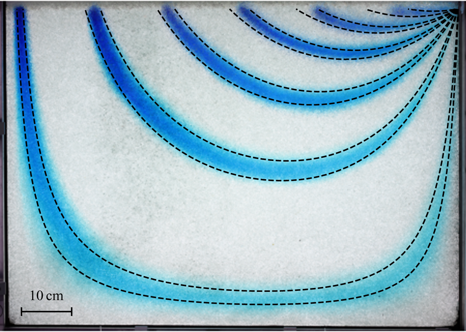
To better illustrate this phenomenon, we merge all the pictures that record the propagation of the dye (approximately 700 images) into a single one by keeping, for each pixel, its darkest value over the course of the experiment. The resulting image reveals the trajectories of each dye parcel in the form of six blue stripes, the width of which is that of the parcel. Each of the two edges of a stripe corresponds to a streamline (figure 4). The curvature of the streamlines confirms that the flow is two-dimensional. The flow even becomes essentially vertical near the upper surface of the aquifer, where the streamlines head downwards. As groundwater enters deeper in the aquifer, its trajectory gradually curves inwards, and reaches its maximum depth. Groundwater then rises towards the aquifer's outlet, where all the streamlines converge. The vertical component of the flow is specially strong for the streamlines that originate far from the outlet. As a result, the further a streamline starts from the outlet, the deeper its excursion below the surface.

In the next section, we derive an approximate analytical expression for the streamlines, and compare it to our observations.
4. Hydraulic head and stream function
4.1. Flow equations
Our experimental aquifer is made of a homogeneous and isotropic porous material. The Reynolds number of the flow is  ${Re} = U d_p/\nu$, where
 $\nu$ is the kinematic viscosity of water, and
 $U$ its typical velocity in the aquifer. Based on the propagation of the dye in our experiment, we find that the latter varies in the range
 $10^{-2}\ \textrm {cm}\ \textrm {s}^{-1}$ to
 $4\times 10^{-1}\ \textrm {cm}\ \textrm {s}^{-1}$, so that
 ${Re}$ varies between
 $10^{-2}$ and
 $0.4$. Groundwater thus flows according to the simplest version of Darcy's law:
 \begin{equation} {\boldsymbol q} ={-} K {\boldsymbol\nabla} \left ( \frac{p}{\rho g} + y \right), \end{equation}
where  $\boldsymbol {q}$,
 $\rho$ and
 $p$, are the flux of water, its density and pressure, respectively. The horizontal and vertical coordinates,
 $x$ and
 $y$, are measured with respect to the position of the aquifer's outlet (figure 1). In steady state, combining Darcy's law and the incompressibility condition yields the Laplace equation,
 \begin{equation} \nabla^2\phi = 0, \end{equation}
where  $\phi = p/\rho g + y$ is the hydraulic head.
To solve it, we must complement (4.2) with boundary conditions. We first assume that the flow does not vary across the experiment; the two Plexiglas® plates thus confine it to a vertical plane. The three walls bounding the aquifer are impervious, and the normal velocity of groundwater vanishes along them:
 \begin{equation} \frac{\partial\phi}{\partial n} = 0, \end{equation}
where  $n$ denotes the direction of the normal to the wall.
We now turn our attention to the water table,  $y=h(x)$. It is the surface where the pressure is atmospheric. Arbitrarily setting the latter to zero, this definition translates into
 \begin{equation} \phi = y \end{equation}
at the free surface ( $y= h(x)$).
When rain falls, the water table deforms to accommodate the input of water. One must therefore deduce its shape from the flow equations: it is part of the solution. This free-boundary problem thus requires an additional boundary condition, which is just the water balance across the water table (Van de Giesen, Parlange & Steenhuis Reference Van de Giesen, Parlange and Steenhuis1994). In steady state, the latter reads
 \begin{equation} \frac{\partial \phi}{\partial y} - \frac{\partial \phi}{\partial x} \frac{\partial h}{\partial x} = \frac{R}{K} \end{equation}
at the free surface ( $y= h(x)$), where the rainfall rate
 $R$ and the hydraulic conductivity
 $K$ have units of velocity.
The Laplace equation (4.2), subjected to the boundary conditions (4.3), (4.4) and (4.5), describes how rainfall drives the flow of groundwater through the aquifer in steady state. In the absence of rainfall ( $R =0$), the water table does not deform (
 $h=0$). In this trivial case, the pressure is hydrostatic (
 $\phi = 0$) and the groundwater remains still.
4.2. Weak rainfall
We could not find any closed-form solution of the system (4.2), (4.3), (4.4) and (4.5). Fortunately, in our experiments, the rainfall rate is much smaller than the hydraulic conductivity, and the ratio of the two,  $R/K$, never exceeds
 $4.1\times 10^{-3}$ (table 1). The same observation often applies in nature, where the average recharge rate is typically much smaller than the conductivity of unconfined aquifers (Haitjema & Mitchell-Bruker Reference Haitjema and Mitchell-Bruker2005; Guérin et al. Reference Guérin, Devauchelle, Robert, Kitou, Dessert, Quiquerez, Allemand and Lajeunesse2019). The ratio of these two quantities is therefore a small parameter, with respect to which we may linearize (4.5). When this ratio is vanishingly small (
 $R/K \ll 1$), the water table is virtually horizontal, and its deformation barely visible (1 cm at most in our experiment). Accordingly, we now linearize the boundary condition at the free surface (4.5) around the hydrostatic solution (
 $h = 0$,
 $\phi = 0$, Dagan Reference Dagan1964):
 \begin{equation} \frac{\partial \phi}{\partial y} = \frac{R}{K}\quad \textrm{in } y= 0. \end{equation}
In the weak-rainfall regime, the flow obeys the Laplace equation (4.2) with boundary conditions (4.3) and (4.6). As anticipated, the elevation of the water table,  $h$, drops out of the equations at this order: we no longer need to solve a Stefan problem. We solve this linear system using complex analysis (Polubarinova-Kochina Reference Polubarinova-Kochina1962). An advantage of doing so is that it provides simultaneously the hydraulic head
 $\phi$ and the stream function
 $\psi$. Accordingly, we introduce the complex coordinate
 $z = x + \textrm {i}y$ (with
 $i^2=-1$), and look for an analytical function
 $\varPhi (z) = \phi (z) + \textrm {i} \psi (z)$ that satisfies the boundary conditions. The stream function
 $\psi$, like the hydraulic head
 $\phi$, are rescaled with the hydraulic conductivity
 $K$ (they both have units of length).
Along the impervious walls ( $x = 0$,
 $x=-L$, and
 $y= -H$), (4.3) translates into
 \begin{equation} \psi = 0, \end{equation}
where we have set the arbitrary constant of the stream function to zero. Using the Cauchy–Riemann relations, we rewrite (4.6) in terms of the stream function, and integrate the result along the  $x$-axis:
 \begin{equation} \psi ={-} \frac{RL}{K} \left(1+\frac{x}{L}\right) \quad \textrm{in } y= 0. \end{equation}
This condition, together with (4.7), means that the stream function is discontinuous at the outlet. This discontinuity is an inevitable consequence of the linearization of the free surface, which reduces the aquifer outlet to a point (§ 4.3). As expected for the stream function, the amplitude  $[\psi ]$ of this discontinuity is the discharge of the aquifer, which matches the rainfall input:
 $KW[\psi ] = Q=RLW$.
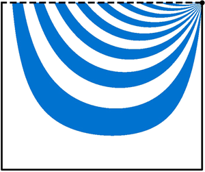
The flow of groundwater in our aquifer thus obeys (4.2) with boundary conditions (4.7) and (4.8). To solve this system, we first note that any periodic function of the form
 \begin{equation} \varPhi_k(z) = \frac{RL}{K} \cosh\left[k {\rm \pi}\left(\frac{\textrm{i}z}{L} - a\right) \right], \end{equation}
where  $k$ is an integer, satisfies boundary condition (4.7) in an aquifer of aspect ratio
 $a=H/L$ (figure 5). Equation (4.9) is not the solution of our problem, however, as it does not fulfil the kinematic condition (4.8) at the water table. Fortunately, our problem is now linear, and we may look for its solution in the form of a series of periodic modes:
 \begin{equation} \varPhi(z) = \sum_{k=1}^{\infty}C_k \varPhi_k(z), \end{equation}
where  $C_k$ are real constants. We now need to find the
 $C_k$ coefficients for which the series converges to boundary condition (4.8) at the surface.
First three modes of the complex velocity potential (4.11) in an aquifer of aspect ratio  $a=1$. (a–c) Dimensionless stream function
 $K \psi /(RL)$ at the free surface (
 $y=0$). (d–f) Streamlines (black dashed line) and hydraulic head (blue shading, normalized to 1).

Noting that, for each mode  $k$, the stream function
 $\psi _k$ reduces to a cosine at the surface, we use a Fourier transform to compute the
 $C_k$ coefficients. This is tantamount to finding the Fourier series of the saw-tooth function – a textbook problem (Farlow Reference Farlow1993). We thus find the expression for the complex velocity potential in the form of a Fourier series:
 \begin{equation} \varPhi(z) ={-} 2\frac{RL}{K}\sum_{k=1}^{\infty} \frac{\cosh\left(k {\rm \pi}(\textrm{i}z/L - a) \right)}{k{\rm \pi} \sinh( k{\rm \pi} a)}. \end{equation}
The imaginary part of this velocity potential yields the stream function  $\psi (x,y)$, the contours of which are streamlines. To draw them, we need to (1) define a numerical grid over the aquifer's extent, (2) evaluate the stream function on this grid, (3) extract the contours of this function. Accordingly, we start by building a triangular mesh of the aquifer, using the internal mesher of FreeFem++ (Hecht (Reference Hecht2012), Python routines available online: https://github.com/odevauchelle/pyFreeFem). Based on (4.11), we then evaluate the stream function on this mesh. Finally, we use the Matplotlib library to extract its contours, which are the streamlines (figure 6). The accuracy of this procedure depends on the mesh size
 $\delta \ell$, and on the truncation of the series (4.11). This truncation generates large, high-frequency oscillations near the singularity, an instance of the Gibbs phenomenon, which we attenuate with the Lanczos
 $\sigma$ factors (Hamming Reference Hamming1973, p. 534). By trial and error, we opt for
 $\delta \ell /L = 1.25\times 10^{-2}$ and
 $100$ modes, a good trade-off between accuracy and computation speed.
Steady-state flow in aquifers of aspect ratio  $a=0.35$,
 $0.7$ (as in our laboratory experiment) and
 $1.4$, respectively, after (4.11). (a–c) Dimensionless travel time of rainwater,
 $\tau ^*$, as a function of relative landing position,
 $x_{start}/L$. Solid blue line: numerical approximation (§ 5.2). Black dashed line : expansion near the outlet, (5.2). (d–f) Streamlines (black dashed lines) and hydraulic head (blue shading).

The streamlines corresponding to each mode of the velocity potential (4.11), when plotted individually, divide the water table between regions where water enters the aquifer, and regions where water seeps out of it (figure 5); the incoming flux balances the outgoing one exactly. The summation of a large number of modes preserves this mass balance, but distributes the flux differently. Rainfall uniformly enters the aquifer through the water table, and all the streamlines converge towards a point sink, through which the entire discharge exits the aquifer (figure 6). The mass balance then requires that the flow velocity diverges at the outlet, thus creating a mathematical singularity. We shall characterize this singularity in the next section.
The streamlines that correspond to (4.11) are consistent with our experimental observations (figure 6). Oriented downward near the water table, they gradually curve as they plunge into the aquifer. Eventually, they rise towards the aquifer's outlet, where they all converge. Streamlines are especially bent near the two stagnation points located in the bottom corners of the aquifer.
A more quantitative comparison with the experiments reveals that the streamlines drawn on figure 4 after (4.11) consistently reproduce the travel of the dye through our laboratory aquifer. This linearized theory even accounts for the thinning of the dye parcel near the bottom of the aquifer (figure 4). These observations support the use of the weak-rainfall approximation in our experiments.
Under this approximation, the intensity of rainfall affects only the norm of the groundwater velocity, leaving the geometry of the flow unchanged. The shape of the streamlines depends solely on the aspect ratio of the aquifer,  $a=H/L$. Not surprisingly, we find that the streamlines approach the horizontal as we decrease the latter (figure 6). Yet, even for a very shallow aquifer, the vertical component of the flow remains predominant near the outlet and near the divide, in contradiction with the Dupuit–Boussinesq approximation (figure 6d).
As the water table bulges to accommodate the rainfall input, the volume of water stored in the aquifer increases. In steady state, the intensity of rainfall thus controls the volume of water the aquifer stores above the outlet. One can easily measure this quantity by collecting all the water that seeps out of the experiment after the rain has stopped. It is therefore tempting to calculate this volume by integrating the elevation of the water table above the outlet along the aquifer's length:
 \begin{equation} V_e = W \int_{{-}L}^{0} h(x)\,{\textrm{d}x}. \end{equation}
In the present theory, we use the boundary condition (4.4) to find the water-table elevation at the free surface,  $h(x) \approx \phi (x, y=0)$. As one might expect, near the drainage divide, the water table lies above the outlet (
 $h>0$). It decreases towards the outlet, however, and eventually plunges below it (
 $h<0$), as the singularity associated with the exit condition takes over the flow (§ 4.3). Although unrealistic, this mathematical behaviour makes it possible for (4.12) to yield a vanishing or even negative volume. In fact, integrating this equation, we find that the positive and negative contributions of
 $h$ compensate for each other exactly (appendix A). Regardless of the rainfall rate or the aquifer's aspect ratio, the volume stored during rainfall always vanishes. Thus, although the weak-rainfall approximation faithfully represents the flow streamlines, it cannot account for the water stored in the aquifer during rainfall. The estimation of this volume requires to solve the original, non-linear Stefan problem.
Our experiments, like the linear theory, are limited to the weak-rainfall regime. At large rainfall rates, we expect that the deformation of the water table will eventually break the linear approximation, thus changing the flow geometry. However, this non-linear regime is beyond the scope of the present paper, and the capacity of our experimental set-up.
4.3. Flow near the outlet
The series expansion of § 4.2 becomes singular near the outlet. To characterize this singularity mathematically, we could expand the modes of the series as  $z$ approaches zero, but we would then find that nested series expansions obscure the issue. Instead, we propose here a longer route that, hopefully, offers a clearer view of the singularity.
The flow near the aquifer's outlet should be insensitive to the position of the bottom wall. Taking advantage of this, we consider an infinitely deep aquifer, by sending the bottom wall to infinity ( $H\rightarrow \infty$). The problem then reduces to the Laplace equation (4.2) with boundary condition (4.6) at the water table, while boundary condition (4.7) applies only along the right and left walls. Using conformal mapping (Polubarinova-Kochina Reference Polubarinova-Kochina1962), we find that the velocity potential then reads (figure 7a)
 \begin{equation} \varPhi \underset{H \to +\infty}{\longrightarrow}\varPhi_{deep} = \frac{2}{\rm \pi}\frac{RL}{K} \left[ \log\left( 1 - \exp({\textrm{i}{\rm \pi} z/L})\right) - \textrm{i} {\rm \pi}\left(\frac{z}{L}+1\right) \right]. \end{equation}
The corresponding streamlines resemble that of an aquifer of finite depth, except near the drainage divide where they go down to infinity (figure 7a).
(a) Flow in an infinitely deep aquifer. (b) Asymptotic regime near the singularity at the aquifer outlet. Black dashed line: streamlines (linearly spaced); blue shading: hydraulic head.  $\theta$ is the inclination of the streamlines with respect to horizontal.

Near the outlet, the flow is also insensitive to the left wall. Accordingly, sending the latter to infinity, or, equivalently, expanding (4.13) about  $z=0$, yields the expression of the velocity potential near the outlet:
 \begin{equation} \varPhi \underset{z \to 0}{\longrightarrow} \varPhi_{outlet} = \frac{RL}{K} \left[ \frac{2}{\rm \pi} \log\left( \frac{z}{L} \right) +\textrm{i} \right]. \end{equation}
As expected for a point sink in a Laplacian field, the velocity potential diverges logarithmically, with a prefactor proportional to the ratio of the discharge per unit width,  $Q/W=RL$, to the conductivity
 $K$ (figure 7b). The corresponding streamlines form spokes converging towards the outlet, in agreement with the trajectory of the dye parcels in our experiment (figure 4). This flow pattern is independent of the prefactor in (4.14). In addition, not too close to the exit grid, the flow is also insensitive to the details of the outlet's geometry. Transposed into a natural setting, this observation means that the river's shape does not affect the far field of the groundwater flow, although it may add to the pressure head a constant, which depends on the water level in the river.
The spoke pattern formed by the streamlines, and their even spacing, means that the flux of water is uniformly distributed around the outlet. The same observation holds at the surface of the aquifer: since the rainfall is uniform, streamlines are evenly spaced there too. The water-mass balance then imposes a linear relation between the inclination of a streamline near the outlet,  $\theta$ (figure 7b), and its entry point into the aquifer,
 $x_{start}$ (figure 6):
 \begin{equation} x_{start} ={-}\frac{2 \theta}{\rm \pi} L. \end{equation}
One sometimes uses a series of boreholes to measure how the chemical composition of groundwater changes with depth (Haria & Shand Reference Haria and Shand2004). Equation (4.15), if it holds in the field, would allow us to relate this depth to the path of groundwater through the aquifer.
Now that we have established a mathematical description of the streamlines, we turn our attention to the time it takes for a fluid parcel to travel along them. Most likely, the outlet singularity, which concerns only the end of the travel, will barely affect this travel time.
5. Travel time
5.1. Travel of a parcel of dye
On average, fluid parcels travel along the streamlines at a velocity equal to the flux of water divided by the aquifer porosity,  ${\boldsymbol q}/s$ (Guyon, Hulin & Petit Reference Guyon, Hulin and Petit2001). Accordingly, the time that a particle needs to move between two points of complex coordinates
 $z_0$ and
 $z_1$ reads:
 \begin{equation} t = \frac{s}{K}\int_{z_0}^{z_1} \frac{\mathrm{d}l}{|\boldsymbol{\nabla} \phi|}, \end{equation}
where the integral follows the streamline that connects  $z_0$ and
 $z_1$ (
 $l$ is the distance along this streamline).
The travel time computed from (5.1) only takes into account the advection by the flow. In reality, the velocity of water varies significantly within a single pore, and between pores (Saffman Reference Saffman1959). The dispersion thus induced is visible in our experiment: the parcels of dye spread out along their path (figure 3). We shall discuss how this dispersion influences the distribution of travel times in § 6. First, however, we ignore its influence, and compute the travel time associated with advection only.
Using (5.1), we compute numerically the positions of the six parcels of dye injected in our experimental aquifer as a function of time. To do so, we extract the shape of the six streamlines that originate from the injection points (§ 4.2). We then evaluate the hydraulic head along their course, compute the magnitude of its gradient, and evaluate integral (5.1) numerically. This procedure yields the travel time as a function of the position along the streamline. It accounts for the motion of the parcels, without any free parameter, but cannot represent their spreading (figure 3). Encouraged by this observation, we now investigate how this travel time depends on where a raindrop lands.
5.2. Travel times
Where a raindrop lands sets the origin,  $x_\textrm {start}$, of the streamline along which it will travel underground. We may therefore calculate the travel time
 $\tau$ of a raindrop by integrating numerically (5.1) along this streamline, as in the previous section. In practice, however, the existence of three singular points – two stagnation points on the left and right corners of the aquifer bottom, and a singularity at the outlet – complicates this calculation. To deal with this problem, we build a mesh of the aquifer that skirts the two stagnation points and the aquifer outlet (figure 8). To do so, we trim three corners off the mesh along circles of radius
 $\epsilon$. Some of the streamlines cut through these circles. Equation (5.1) provides the contribution to the travel time of the segments located outside the corresponding disks. To complete the calculation, we need to work out the travel time through the disk that surrounds each singularity.
Mesh (grey triangles) of an aquifer skirting the two stagnation points and the aquifer outlet (grey disks). Black dotted lines: streamlines (logarithmically spaced). Blue shading: hydraulic head. The aquifer aspect ratio is  $a=0.5$. For illustration, we set the radius of the quarter-circles to
 $\epsilon /L= 0.1$ and the maximum mesh size to
 $\delta \ell /L =0.025$. In practice, travel times are calculated with
 $\epsilon /L= 0.05$ and
 $\delta \ell /L =0.0125$.

Replacing the velocity potential with its expression near the outlet (4.14) in (5.1), we compute the time water takes to cross the disk surrounding the outlet (figure 8):
 \begin{equation} \tau_{outlet} = \frac{\rm \pi}{4} \frac{sL}{R}\left(\frac{\epsilon}{L}\right)^2. \end{equation}
The radial symmetry of the logarithmic singularity makes  $\tau _\textrm {outlet}$ independent of the direction along which the streamline approaches the outlet.
We now turn our attention to the two stagnation points (figure 8). To compute the integral in (5.1), we first note that  $|{\boldsymbol \nabla } \phi | = |\varPhi '|$ and
 $\textrm {d} l = |\textrm {d} z| = |\textrm {d} \varPhi | / |\varPhi '|$, where
 $'$ denotes the complex derivative. Along a streamline, the stream function is constant, while the hydraulic head decreases, so
 $|\textrm {d}\varPhi | = -\textrm {d}\phi$. Combining all these expressions, we rewrite (5.1) as
 \begin{equation} \tau_s ={-} \frac{s}{K}\int_{\phi_{in}}^{\phi_{out}} \frac{\textrm{d}\phi}{|\varPhi^{\prime}|^2}, \end{equation}
where  $\phi _{in}$ and
 $\phi _{out}$ are the values of the hydraulic head at the entry and exit points of the disk, respectively. Near a stagnation point, the velocity potential is dominated by the first mode of (4.11). Taking advantage of this, we approximate the velocity potential by this mode only. Expanding the latter near the stagnation point, we obtain the following expression for the velocity potential:
 \begin{equation} \varPhi_s = \phi_c \left[ 1- \frac{{\rm \pi}^2}{2} \left(\frac{z-z_s}{L}\right)^2 \right], \end{equation}
where  $z_s$ is the position of the stagnation point (
 $z_s = -L-\textrm {i}H$ in the lower-left corner and
 $z_s =-\textrm {i}H$ in the lower-right one). The hydraulic head at the stagnation point,
 $\phi _c$, is that of the far field, namely
 $\phi _c = \Re (\varPhi (z_s))$.
Writing the derivative of the potential (5.4) as a function of the potential  $\varPhi _s$ itself, namely
 \begin{equation} \varPhi_s^{\prime} ={-} \sqrt{2}{\rm \pi} \frac{\phi_c}{L} ~\sqrt{1 - \frac{\varPhi_s}{\phi_c}}, \end{equation}
allows us to turn the curvilinear integral (5.3) into a classical one. Integrating the latter over  $\phi$, we find that the time spent by a fluid parcel inside the disk surrounding a stagnation point reads
 \begin{equation} \tau_s = \frac{sL}{R} \frac{\sinh({\rm \pi} a)}{2{\rm \pi}} \left| \textrm{asinh}\left( \frac{ \phi_{in} - \phi_c}{\psi_0}\right) \right|, \end{equation}
where  $\psi _0$ defines the streamline along which the water parcel travels.
We can now evaluate the travel time of water through the aquifer by adding to integral (5.1) the contributions of the outlet (5.2) and, if need be, that of the two stagnation points (5.6). The accuracy of this calculation depends on the radius of the quarter-circles,  $\epsilon$, and on the maximum mesh size
 $\delta \ell$. By trial and error, we choose
 $\delta \ell /L = 1.25\times 10^{-2}$ and
 $\epsilon =0.05$.
The mean travel time of water in the aquifer is the ratio of the volume of water it contains to its discharge:  $\langle \tau \rangle = saL/R$ (Zwietering Reference Zwietering1959; Nauman & Buffham Reference Nauman and Buffham1983). This expression, which resembles a simple definition, is actually an exact consequence of the water-mass balance, combined with Green's theorem (appendix B). In the following, we rescale all travel times with this average, thus introducing the dimensionless travel time
 $\tau ^* = \tau /\langle \tau \rangle$.
Figure 6(a–c) shows the dimensionless travel time  $\tau ^*$ of a raindrop as a function of its landing point,
 $x_{start}$, for several values of the aquifer's aspect ratio. We find that
 $\tau ^*$ increases continuously with the distance
 $|x_{start}|$ that separates the landing point from the aquifer outlet. A careful examination of its variation reveals two singularities: the travel time vanishes near the outlet, and diverges near the divide. We shall derive the asymptotic expressions that account for these regimes in § 5.3. Before that, however, we compare our theory to the travel time of dye in our experiment.
To estimate this travel time, we use the images that record the propagation of the dye (§ 3), and decompose each of them into their hue, saturation and value in the range  $[0,255]$. We select pixels with a saturation above 40 to ensure that their hue is well-defined, and retain the ones that fall into the hue range that corresponds to the colour of the dye (
 $[80,130]$). This procedure yields a series of well-contrasted pictures, where the parcels of dye are highlighted. Using these images, we measure the time at which the front of each parcel reaches the aquifer outlet, and the time at which its rear end finally leaves it. We then estimate the average travel time of the parcel as the mean of these two times,
 $\tau$. Their difference corresponds to the exit duration,
 ${\rm \Delta} \tau$, which we use as an estimate of the measurement dispersion. In fact, the latter results from pore-scale dispersion, a phenomenon we shall address in more detail in § 6. Figure 9 compares our experiments to the theory. Although the latter only accounts for the advection by the flow, we find that it matches our observations. Encouraged by this result, we now examine the two asymptotic regimes that represent the behaviour of the travel time near the singularity, and near the outlet.
Dimensionless travel time of a parcel of dye,  $\tau ^*$, as a function of the distance to the outlet
 $-x_\textrm {start}/L$ (lower axis). Upper axis: streamline inclination at the outlet,
 $\theta$. Blue markers: experimental runs (table 1). Vertical error bars indicate the exit duration,
 ${\rm \Delta} \tau /\langle \tau \rangle$; horizontal ones indicate initial width of the parcel. Coloured lines: theoretical travel times after § 5.2 for aspect ratios
 $a=0.35$ (green),
 $0.7$ (blue, our laboratory experiment) and
 $1.4$ (orange).

5.3. Asymptotic regimes
When a rain drop lands near the outlet, its travel is dominated by the singularity that accelerates the flow towards the exit point. According to (5.2), the duration of this travel decreases as the square of the distance that separates its landing point from the outlet:
 \begin{equation} \tau^* = \frac{\rm \pi}{4a}\left(\frac{x_{start}}{L}\right)^2. \end{equation}
Figure 10(a) shows that our experiment conforms to this asymptotic behaviour.
Travel times through a rectangle aquifer. (a,b) Dimensionless travel time,  $\tau ^*$, as a function of distance to outlet,
 $-x_{start}/L$, and distance to divide,
 $(L+x_{start})/L$. Coloured lines: theoretical travel times, after § 5.2. Black dashed lines: asymptotic regimes (5.7) and (5.8). Blue markers: experimental data (same symbols as in figure 9), vertical error bars indicate the exit duration,
 ${\rm \Delta} \tau /\langle \tau \rangle$, horizontal ones indicate the initial width of the parcel. (c,d) Probability density functions (PDF) of travel times,
 $f(\tau ^*)$, for several aspect ratios. Black dashed line: asymptotic regimes (5.10) and (5.11).

To the contrary, the travel time diverges near the left-hand wall of the aquifer, which simulates a drainage divide (figure 6a–c). To account for this behaviour, we note that a streamline originating near the divide remains close to the walls along its entire course (figure 6d–f). In this region, the velocity potential is dominated by the first mode of (4.11). Taking again advantage of this observation, we approximate the velocity potential by its first mode,  $\varPhi _1$, and use (5.3) to calculate the corresponding travel time. Following a procedure similar to the one applied to the stagnation points in § 5.2, we find the following expression for the travel time near the drainage divide (appendix C):
 \begin{equation} \tau^* \approx{-} \frac{\sinh({\rm \pi} a)}{{\rm \pi} a} \left[ \log\left( 1 + \frac{x_{start}}{L} \right) - \log \left(\frac{4}{1+\cosh({\rm \pi} a) } \right) \right], \end{equation}
which is a good approximation of the actual travel time (figure 10b). As expected, (5.8) features, at leading order, the logarithmic divergence that is the signature of the stagnation points. It also bears the mark of the aspect ratio of the aquifer, which affects both the prefactor of the logarithm, and the additive constant.
5.4. Distribution of travel times
In our experiment, rain falls uniformly onto the aquifer's surface. We may thus write the probability density function (PDF) of travel times as:
 \begin{equation} f(\tau^*) ={-} \frac{1}{L}\frac{\textrm{d}x_{start}}{\textrm{d}\tau^*}. \end{equation}
This expression is but a recasting of the function that relates the travel time of a drop of water to its landing spot.
We approximate (5.9) numerically, based on the results of § 5.2, and plot it for different values of the aspect ratio (figure 10c). The resulting distributions diverge at the origin. From there, they gradually decrease at a rate which depends on the aspect ratio of the aquifer.
Short travel times correspond to raindrops entering the aquifer near the outlet. Accordingly, the expression of the travel time near the outlet (5.7), combined with (5.9), yields the short-time behaviour of the PDF:
 \begin{equation} f(\tau^*) \sim \left( \frac{a}{\rm \pi}\right)^{1/2} \tau^{*-1/2}. \end{equation}
This expansion consistently represents the short-time behaviour of the numerical PDF (figure 10c). The divergence of the latter at short times is a consequence of the acceleration of the flow near the outlet.
Long travels, on the contrary, correspond to raindrops entering the aquifer near the drainage divide. Streamlines originating from this area entrain their water near the two stagnation points, where it lingers for a logarithmically long time. Accordingly, we now combine the travel time near the drainage divide (5.8) with (5.9). We find that the tail of each PDF decreases exponentially, according to
 \begin{equation} f(\tau^*) \sim \frac{4{\rm \pi} a}{\sinh({\rm \pi} a) (1+\cosh({\rm \pi} a))}\exp({-\tau^*/\tau^*_c}), \end{equation}
with a characteristic dimensionless time
 \begin{equation} \tau^*_c = \frac{\sinh({\rm \pi} a)}{{\rm \pi} a}. \end{equation}
Again, this expansion accords with the numerical PDF (figure 10d). As anticipated, the characteristic time  $\tau ^*_c$ increases with the aquifer's aspect ratio: deep aquifers induce long travels. In particular,
 $\tau ^*_c$ tends to infinity for an infinitely deep aquifer, whereas it tends towards
 $1$ for a shallow one (
 $a=0$). In short, the tail of the travel-time distribution depends primarily on the aspect ratio of the aquifer.
Although it only accounts for the advection by the flow, the above theory proves a fair representation of our experiment: this approximation suffices to reproduce the travel of individual parcels of dye (figures 3 and 9). In reality, however, the pore-scale hydrodynamic dispersion affects the travel time of groundwater. In the next section, we evaluate the magnitude of its contribution.
6. Hydrodynamic dispersion
Hydrodynamic dispersion gradually spreads a parcel of dye as it travels along its streamline (figure 3). In terms of travel time, this spreading becomes a dispersion time,  ${\rm \Delta} \tau$, defined as the time separating the moment when the front of the parcel reaches the aquifer's outlet, from the moment it has left it entirely. In § 5.2, we estimated this dispersion time, together with the average travel time, for each parcel of dye in our experiment. We now compare these two quantities, and find that the ratio of the dispersion time to the average travel time varies in the range
 ${\rm \Delta} \tau /\tau \approx 0.4\text {--}1.3$: hydrodynamic dispersion indeed affects the propagation of dye through the aquifer (figure 11).


Our measurements also reveal that the ratio of the dispersion time to the travel time,  ${\rm \Delta} \tau /\tau$, decreases with
 $x_{start}$ (figure 11). The relative influence of hydrodynamic dispersion therefore decreases with the length of the travel. We now interpret this observation with scaling arguments. The time necessary for a parcel of dye to cross the aquifer's outlet scales like
 ${\rm \Delta} \tau \sim \ell _p/U,$ where
 $\ell _p$ is the length of the parcel when it reaches the outlet, and
 $U$ is the characteristic velocity at which the parcel travels along the streamline. Assuming that the length of a streamline is proportional to the position of its origin,
 $-x_{start}$, this velocity scales like
 $U \sim -x_{start}/\tau .$ As the pore-scale dispersion spreads the parcel, the length of the latter scales like
 $\ell _p \sim \sqrt {D \tau },$ where
 $D$ is the dispersion coefficient. Neglecting molecular diffusion, this coefficient is the product of the fluid velocity
 $U$ and a dispersion length
 $\lambda$ (
 $D = \lambda U$, Hillel Reference Hillel2003). In a homogeneous aquifer, this dispersion length is proportional to the pore size,
 $d_p$. Combining these four equations, we find that
 ${\rm \Delta} \tau /\tau$ decreases with the distance
 $x_{start}$ according to
 \begin{equation} \frac{{\rm \Delta} \tau}{\tau} \approx \left( \frac{\lambda}{-x_{start} }\right)^{1/2}. \end{equation}
A fit of (6.1) to our data consistently reproduces the evolution of the ratio  ${\rm \Delta} \tau /\tau$ in our experiment, with
 $\lambda \approx 1288~d_p \approx 12.9\ \textrm {cm}$, a value close to that measured in sand columns (De Marsily Reference De Marsily1986).
Equation (6.1) indicates that the relative importance of hydrodynamic dispersion at the pore scale with respect to advection at the aquifer scale is essentially governed by the ratio of the dispersion length,  $\lambda$, to the distance,
 $x_{start}$, that separates the landing point of the raindrop from the aquifer's outlet.
7. Conclusion
The experiments presented in this paper reveal the flow pattern in a deep, unconfined aquifer recharged by rainfall. Since the outlet stands high above the aquifer's bottom, groundwater needs to go up to reach it, which breaks down the Dupuit–Boussinesq approximation. We find an analytical expression of the velocity potential, in the form of an infinite series of modes, which accounts for the shape of the experimental streamlines. This linear theory represents correctly the travel of water through the aquifer, provided that the intensity of rainfall is much less than the aquifer's conductivity, a condition often met in nature (Haitjema & Mitchell-Bruker Reference Haitjema and Mitchell-Bruker2005).
The underground fate of a raindrop depends on where its enters the aquifer. A raindrop that lands near the outlet flows out almost immediately. On the contrary, the trajectory of a drop fallen near the drainage divide reaches down to the bottom of the aquifer, before it rises up towards the outlet. The duration of this long travel is further increased by the stagnation points that drainage divides generate. These stagnation points control the tail of the travel-time distribution, which we find to decrease exponentially, with a characteristic time that depends on the aquifer's aspect ratio.
Our theory bears similarity to the model of Toth (Reference Toth1963). Like us, Toth restricts his analysis to small deformations of the water table, and linearizes the boundary condition at the free surface accordingly. However, whereas our theory explicitly accounts for the rainfall rate that recharges the aquifer, Toth (Reference Toth1963) imposes the elevation of the water table. Assuming that the latter inherits its shape from the land above it, he represents it with an uniform slope modulated by a sinusoidal wave (Toth Reference Toth1963, equation (5d)). The sine mimics the hills and depressions of the land surface, while the slope represents the regional gradient. If the latter vanishes, the solution found by Toth (his equation (6)) coincides with the first mode of equation (4.11) of the present paper. As this mode dominates the flow far below the water table, both models yield the same trajectory for a droplet fallen near the drainage divide. Toth's model can therefore account for the tail of the travel-time distribution. Closer to the surface, however, Toth's model departs from the present theory, and, therefore, cannot represent the faster paths we observe in our experiment.
Our estimate of the travel time only takes into account advection by the flow. In reality, hydrodynamic dispersion affects the distribution of travel times. Our experiments indicate that the magnitude of this effect depends on the ratio of a dispersion length, proportional to the pore size, to the length of the streamline. In the field, these lengths most likely differ by several orders of magnitude, and we thus speculate that pore-scale dispersion is negligible.
Near the aquifer's outlet, the streamlines flow radially, with an inclination that depends on the location of their origin. This result, if it holds in nature, provides a simple method to reconstruct the distribution of travel times through an aquifer. Indeed, a series of boreholes, drilled at different depths near the edge of a river, would collect groundwater travelling along different streamlines. Sampling water in each borehole and measuring the time it spent underground, based on isotopic ratios or conservative tracers, could thus yield the distribution of travel times through the aquifer. One might then infer the aquifer's effective depth from the characteristic time of the distribution's tail.
Our experiments are based on the measurement of the position and size of dye parcels travelling through the aquifer. Such measurements are hardly possible in the field. Instead, one usually injects a chemical tracer into a well, and records the evolution of its concentration in another downstream one. The breakthrough curve, i.e. the time series of the concentration in the second well, is then used to infer the flow within the aquifer (Gelhar, Welty & Rehfeldt Reference Gelhar, Welty and Rehfeldt1992). In our experiment, the absorption of light by the dye might, in principle, allow us to follow its distribution in the aquifer. This method would allow us to produce breakthrough curves, and to compare them with field measurements.
Finally, our experiments reveal that the reaction of the water table to rainfall is considerably faster in a deep aquifer than in a shallow one. This observation calls for an investigation of the stormflow regime, which is crucial to flood forecasting (Guérin et al. Reference Guérin, Devauchelle, Robert, Kitou, Dessert, Quiquerez, Allemand and Lajeunesse2019). Our experiments suggest that this regime mobilizes the entire volume of the aquifer instantly, but a theory of this dynamical regime remains to be established.
Supplementary movie
Supplementary movie is available at https://doi.org/10.1017/jfm.2021.221.
Acknowledgements
We are grateful to S. Deboeuf, F. James, P. Gondret, Y. Meheust, F. Métivier, J. Neufeld, C. Soulaine and P. Szymczak for their insightful comments. We thank M. Vulliet and M. Colledge, who performed some of the experiments as part of a tutored project. We also express our gratitude to O. Bour for his guidance through the travel-time literature. Finally, we thank an anonymous referee for suggesting the use of the Lanczos sigma factors.
Declaration of interests
The authors report no conflict of interest.
Appendix A. Volume of groundwater stored in the aquifer
During rainfall, the water table bulges, and the volume of water stored in the aquifer increases. In steady state, the volume of water that the aquifer stores above the outlet reads
 \begin{equation} V_e = W \int_{{-}L}^{0} h(x) \,{\textrm{d}x}, \end{equation}
where  $h(x)$ is the elevation of the water table with respect to the outlet. At leading order, it is the hydraulic head at
 $y=0$:
 $h(x) = \phi (x, y=0)$. The stored volume is therefore
 \begin{equation} V_e = W \int_{{-}L}^{0} \phi(x, y=0) \,{\textrm{d}x}. \end{equation}
To calculate this integral, we first rewrite it in terms of the complex potential,
 \begin{equation} V_e = W \Re\left\{ \int_{{-}L}^{0} \varPhi(z)\,\textrm{d} z \right\}. \end{equation}
Taking advantage of the Cauchy integral theorem, we evaluate this integral along a contour that follows the aquifer's walls:
 \begin{equation} V_e = \Re\left\{ \int_{{-}L}^{{-}L(1+\textrm{i}a)} \varPhi(z)\,\textrm{d} z + \int_{{-}L(1+\textrm{i}a)}^{{-}Lia} \varPhi(z)\,\textrm{d} z + \int_{{-}Lia}^{0} \varPhi(z)\,\textrm{d} z\right\}. \end{equation}
As only the second integral has a finite real part, the stored volume simplifies into
 \begin{equation} V_e = \Re\left\{ \int_{{-}L(1+\textrm{i}a)}^{{-}Lia} \varPhi(z)\,\textrm{d} z \right\}. \end{equation}
Using (4.11), we rewrite this integral as
 \begin{equation} V_e ={-} 2\frac{RL}{K}\sum_{k=1}^{\infty}\frac{1}{k{\rm \pi} \sinh( k{\rm \pi} a ) } \int_{{-}L}^{0} \cos\left( \frac{k {\rm \pi}x}{L} \right) {\textrm{d}x}, \end{equation}
which yields
 \begin{equation} V_e = 0. \end{equation}
In the weak-rainfall approximation, the volume of water stored in the aquifer during rainfall is zero. This, of course, is only a first-order result. To find how much water a deep aquifer can accommodate in steady state, we need to return to the original, non-linear Stefan problem.
Appendix B. Mean travel time of water in the aquifer
As the flow is in steady state, we can attribute an age  $a$ to each point in our aquifer, that corresponds to the time it takes for water to travel from the surface to this point. The mean travel time of groundwater is the flux of age through the contour
 $\varGamma$ that bounds the aquifer, normalized by the outlet discharge,
 $Q = RLW$:
 \begin{equation} \langle \tau \rangle = \frac{W}{Q} \oint_\varGamma a \bf{q}\cdot \bf{n}\,\textrm{d} l, \end{equation}
where  $l$ is the distance along the contour of the aquifer. Using Gauss's theorem, we rewrite (B1) as
 \begin{equation} \langle \tau \rangle = \frac{W}{Q} \left( \iint_\varSigma \bf{q}\boldsymbol{\cdot} \boldsymbol{\nabla} a \,\textrm{d}\varSigma - \iint_\varSigma a \boldsymbol{\nabla}\boldsymbol{\cdot}\bf{q} \,\textrm{d}\varSigma \right), \end{equation}
where  $\varSigma$ is the flow domain, that is, a vertical section of the aquifer of area
 $aL^2$ (figure 1).
As a parcel of groundwater travels through the aquifer, its age  $a$ increases with time according to
 \begin{equation} \frac{\textrm{D} a}{\textrm{D} t} = \frac{\partial a}{\partial t} + \bf{v}\boldsymbol{\cdot}\boldsymbol{\nabla}{a} = 1, \end{equation}
where  $\bf{v} = \bf{q}/s$ is the average velocity of the parcel (Davis & Bentley Reference Davis and Bentley1982; Varni & Carrera Reference Varni and Carrera1998). In steady state, the above equation becomes
 \begin{equation} \bf{q}\boldsymbol{\cdot}\boldsymbol{\nabla}{a} = s. \end{equation}
Combining (B2), (B4) and the incompressibility condition ( $\boldsymbol {\nabla }\boldsymbol {\cdot }\bf{q} =0$), we finally get the expression of the mean travel time:
 \begin{equation} \langle \tau \rangle = \frac{saL}{R}. \end{equation}
The mean travel time is therefore equal to the volume of water in the aquifer divided by its discharge (Zwietering Reference Zwietering1959; Nauman & Buffham Reference Nauman and Buffham1983). It is independent of the aquifer's shape.
Appendix C. Expansion of the travel time near the drainage divide
A streamline originating near the divide remains close to the walls, where the velocity potential is dominated by the first mode of (4.11) (figure 6d–f). We therefore approximate the velocity potential by  $\varPhi _1$, and use (5.3) to express the dimensionless travel time:
 \begin{equation} \tau^* ={-} \frac{2R}{aLK} \int_{\phi_{in}}^{\phi_{out}} \frac{\textrm{d}\phi_1}{|\varPhi_1^{\prime}|^2}, \end{equation}
where we integrate along the streamline. Here, we invoked the symmetry of the first mode, and integrated between the origin of the streamline,  $z_{in} = -L+\delta$, and its mid-course point,
 $z_{out} = -L/2 + \textrm {i} (\delta -H)$, where
 $\delta \ll L$ is the distance separating the origin of the streamline from the divide.
Expressing  $\varPhi _1'$ as a function of
 $\varPhi _1$, we turn the above curvilinear integral into a classical one:
 \begin{equation} \tau^* ={-} \frac{2 \sinh({\rm \pi} a)}{{\rm \pi} a} \int_{\phi_{r,in}}^{\phi_{r,out}} \frac{\textrm{d}\phi_r}{|\varPhi_r| | 2 + \varPhi_r |}, \end{equation}
where we introduced the rescaled potential  $\varPhi _r = \phi _r + \textrm {i} \psi _r = \cosh ( {\rm \pi}(\textrm {i}z/L-a) ) -1$. The bounds of this integral are the values of
 $\phi _r$ in
 $z_{in}$ and
 $z_{out}$.
Near the stagnation point, both  $\phi _r$ and
 $\psi _r$ are small. At leading order, the integrand
 $I(\phi _r, \psi _r)$ of (C2) becomes:
 \begin{equation} I \approx I_0 = \frac{1}{2 \vert \varPhi_r \vert} = \frac{1}{2\sqrt{\phi_r^{2} + \psi_r^{2}}}. \end{equation}
As expected, this expression is not integrable when  $\psi _r$ vanishes: the travel time diverges as the flow line approaches the stagnation point. Using the above expression only, the integral of (C2) has a closed-form expression, namely
 \begin{equation} \tau_0^* ={-} \frac{\sinh({\rm \pi} a)}{{\rm \pi} a} \left(\mathrm{asinh} \left( \frac{ \phi_{r,in} }{ \psi_r }\right) - \mathrm{asinh} \left( \frac{\phi_{r,out}}{ \psi_r }\right) \right), \end{equation}
which diverges logarithmically as  $\psi _r$ vanishes, or equivalently, as the landing point of a raindrop approaches the divide:
 \begin{equation} \tau_0^* \approx{-} \frac{\sinh({\rm \pi} a)}{{\rm \pi} a} \log\left( 1 + \frac{x_{start}}{L} \right). \end{equation}
The logarithmic divergence (C5) accounts for the behaviour of the travel time near the divide, but only within an additive constant,  $\tau ^*_1$. To calculate this constant, we subtract the singularity from the leading order integrand:
 \begin{equation} I-I_0 = \frac{2 - \vert 2 + \varPhi_r \vert}{2 \vert \varPhi_r \vert \vert 2+ \varPhi_r\vert}. \end{equation}
By design, this quantity does not diverge as  $\psi _r$ vanishes, and we thus approximate it with
 \begin{equation} I-I_0 \approx{-} \frac{ \textrm{sign} ( \phi_r ) }{2(2+\phi_r)}. \end{equation}
Integrating the latter between  $\phi _{r,in}= \cosh ( {\rm \pi}a) -1$ and
 $\phi _{r,out}=-1$ (the former is positive, and the latter negative) yields the constant we are looking for:
 \begin{equation} \tau^*_1 = \frac{\sinh({\rm \pi} a)}{{\rm \pi} a} \log \left( \frac{4}{1+\cosh({\rm \pi} a) } \right). \end{equation}
Adding (C5) and (C8) yields the expansion of the travel time near the drainage divide, (5.8).