

1. Introduction
Displacement gradients in deformable media such as fluids increase the length and area of material lines and surfaces: an initially isotropic blob of a substance advected by the flow typically elongates while its transverse size compresses. Building on this fact, the lamellar representation of mixing (Batchelor Reference Batchelor1959; Ranz Reference Ranz1979) has proven to be an enlightening and fruitful vision to solve a variety of problems (Villermaux Reference Villermaux2019) including those, beyond conserved scalar mixing, involving a chemical reaction (Gibson & Libby Reference Gibson and Libby1972; Ou & Ranz Reference Ou and Ranz1983; Bandopadhyay et al. Reference Bandopadhyay, Le Borgne, Méheust and Dentz2017; Perez, Hidalgo & Dentz Reference Perez, Hidalgo and Dentz2019; Seonkyoo, Dentz & Kang Reference Seonkyoo, Dentz and Kang2021).
However, with a few exceptions (Larralde et al. Reference Larralde, Araujo, Havlin and Stanley1992; Bandopadhyay et al. Reference Bandopadhyay, Le Borgne, Méheust and Dentz2017, in particular), the canonical bimolecular reaction  ${\rm {A}} + {\rm B} \longrightarrow {\rm C}$ between segregated reactants A and B has mainly been envisaged in the fast chemistry limit, meaning that the rate of chemical conversion, which in that case occurs within a sharp interface between the reactants, coincides with the rate at which they interpenetrate at the molecular level (with characteristic time
 $t_s$, see below), and not by chemical kinetics (characteristic time
 $t_c$). There are, however, multiple original regimes associated with finite Damköhler numbers
 \begin{equation} Da=t_s/t_c, \end{equation}
as illustrated by the recent experiments on a still substrate by Guilbert, Almarcha & Villermaux (Reference Guilbert, Almarcha and Villermaux2021), for instance.
In order to complement the phenomenology on the subject, we study here a new chemical reaction with finite, tunable kinetics (Guilbert et al. Reference Guilbert, Almarcha and Villermaux2021) on a deforming substrate in the simple shear geometry where lamellae mixing has been documented in detail (Souzy et al. Reference Souzy, Zaier, Lhuissier, Le Borgne and Metzger2018), by investigating the coupling between shear intensity and chemical reactivity for a range of  $Da$, and initial conditions.
The Ranz transformation (Ranz Reference Ranz1979), which fundamentally (and elegantly) reduces an advection-diffusion problem to a simple diffusion one in suitable space and time variables is here generalized to problems involving a localized source in space, and is shown to be a useful tool to understand the various chemical production regimes observed in the experiments.
2. Experimental set-up, chemical reaction, protocol
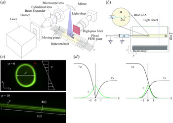
The experimental set-up, shown in figure 1, is both versatile and precise, and is suited to basic mixing studies (Souzy et al. Reference Souzy, Lhuissier, Villermaux and Metzger2017, Reference Souzy, Zaier, Lhuissier, Le Borgne and Metzger2018; Turuban, Lhuissier & Metzger Reference Turuban, Lhuissier and Metzger2021). It consists of a cell formed by two parallel Plexiglas plates 85 mm long, 25 mm wide separated by an  $h=3$ mm gap enclosing a liquid. The liquid layer is sheared by imposing to the plates an opposite movement at the same speed thanks to two translation tables. The cell, sealed at both ends by joints and on the sides by two transparent Plexiglas walls mounted on the bottom plate, is illuminated from the top by a thin (approximately 10 to
 $15 \ \mathrm {\mu }{\rm m}$ thick) laser sheet, expanded from a 488 nm laser beam by a cylindrical lens. This laser sheet is collimated and focused using a microscope lens before being reflected by a
 $45^{\circ }$ mirror to shine it through the shear cell. An optical trap made of the juxtaposition of a hundred razor blades positioned underneath the lower Plexiglas plate minimizes unwanted reflections. To prevent photobleaching, the intensity of the laser is lowered to 500 mW and image acquisition is synchronized with a shutter opening at the acquisition instants only. Perpendicular to the cell, a camera with a macro lens provides an image resolution of
 $0.8\ \mathrm {\mu }{\rm m}\ {\rm pixel}^{-1}$. A high-pass filter positioned in front of the camera lens suppresses direct reflections from the laser.
(a) Schematic of the set-up. (b) Side view of the shear cell and detail of the injection method. (c) Blob of A with diameter  $d$ in the cell filled with B subjected to a shear rate
 $\gamma$. At
 $\gamma t = 0$, the interface between A and B is smeared (the green contour) over a width
 $s_0$ at its periphery. The blob stretches and tilts under shear (length
 $\ell (t)$ shown at
 $\gamma t = 10$) while its borders are close-to-parallel lamellae of width ь(t) and normal
 $n$. (d) Concentration profiles across a lamella: (a,c) thin reaction zone (
 $Da>1$,
 $c$ given by (3.10)), (b,d) diffusive interpenetration before reaction (
 $Da<1$,
 $c$ given by (3.14)).

2.1. Chemical reaction and fluids
We use a second-order irreversible reaction (Guilbert et al. Reference Guilbert, Almarcha and Villermaux2021) between two transparent reactants, namely fluorescin (labelled A) and potassium ferricyanide (labelled B), producing fluorescein (labelled F) which is fluorescent in water (figure 1c). This reaction has a production rate per unit volume  $\dot {c} = kc_Ac_B$ with
 $c_A$,
 $c_B$ the reactants’ concentrations,
 $c$ that of the product and
 $k = 11\ {\rm mol}^{-1}\ {\rm l}\ {\rm s}^{-1}$ the kinetic constant at
 $20\,^{\circ }{\rm C}$ in water. Operating with initial concentrations such that
 $c_{B0}/c_{A0} \gg 1$, the reaction kinetics is of a pseudo-first-order type, with reaction time
 $t_c$:
 \begin{equation} t_c = \left( kc_{B0} \right)^{{-}1},\quad \mbox{so that}\ c = c_{A0}\left(1-{\rm e}^{{-}t/t_c}\right) \end{equation}
when the reactants are initially ideally mixed. By varying the concentration of  $c_{B0}$ and/or the viscosity of the solutions, the reaction time
 $t_c$ can be varied over several decades (Guilbert et al. Reference Guilbert, Almarcha and Villermaux2021, for details). The solutions temperature
 $T=23\,^{\circ }{\rm C}$,
 ${\rm pH}=12$ and the initial concentration
 $c_{A0}=3\times 10^{-5}\ {\rm mol}\ {\rm l}^{-1}$ are kept constant.
To prevent leaks at the plates’ edges, we use a fairly viscous liquid. The solutions used are a mixture of water and UCON oil (Ucon 2021) with two different volume fractions, each corresponding to a viscosity of  $\eta$ of
 $2$ Pa s and
 $1 \times 10^{-1} {\rm Pa}\ {\rm s}$. The corresponding diffusion coefficients of each species are
 $D_{F}=D_{A} = 1 \times 10^{-11}\ {\rm m}^2\ {\rm s}^{-1}$,
 $D_{B}= 2 \times 10^{-11}\ {\rm m}^2\ {\rm s}^{-1}$ and
 $D_{F}=D_{A} = 4 \times 10^{-11}\ {\rm m}^2\ {\rm s}^{-1}$,
 $D_{B}= 2 \times 10^{-10} \ {\rm m}^2\ {\rm s}^{-1}$, while the kinetic constants are
 $k=4.7 \times 10^{-2}\ {\rm mol}^{-1}\ {\rm l}\ {\rm s}^{-1}$ and
 $k=1.1\ {\rm mol}^{-1}\ {\rm l}\ {\rm s}^{-1}$, respectively.
2.2. Protocol
The cell is filled with a solution of B. One of the side plates is fitted with a 0.7 mm hole through which the needle (0.5 mm in diameter) of a syringe containing a solution of A is inserted manually across the cell, in the  $y$-direction perpendicular to the shear direction, 1 mm behind the laser sheet. The syringe is then gently removed back approximately 1 cm as its plunger is kept fixed, leaving a cylinder of A in the B solution along the
 $y$-axis. The intercept of this cylinder with the laser sheet is a disk (that we call blob) with diameter
 $d$ between
 $0.5$ and
 $1$ mm. Once injection is completed, the hole is sealed with an adhesive paste. The translation tables and the camera, synchronized with the laser shutter, are then immediately switched on. The paramount sharp focusing of the camera lens on the laser sheet is ensured before each experiment.
2.3. Operating and initial conditions
The injection of the A blob into the B medium is made quickly, but is not instantaneous. The operations described above (needle injection, translation tables set-up, etc…) last for at least 5 s. Therefore, at  $t=0$ when the shear is set in, reaction has necessarily already started to occur, as manifested by the fluorescent border marking the blob contour (figure 1c), evidencing that some fluorescent product F has been formed during the injection phase. When the blob is sheared, the concentration profiles of A and B are therefore not perfectly sharp, but depleted over a smooth cross-over of width
 $s_0$, function of the injection procedure and waiting time, which may be extremely thin, but is nevertheless always present. The ‘reservoir’ of reactant A is, however, only affected at is border, since
 $s_0$ is always much smaller than the blob size
 $d$.
The shear rate  $\gamma =V/h$ is imposed by the net translational velocity between the plates
 $V$, divided by the gap width
 $h= 3 \times 10^{-3}$ m, and can be varied over
 $0.001<\gamma <10\ {\rm s}^{-1}$. The time needed to reach a steady value of
 $\gamma$ from the plates at rest is of order
 $h^2/\nu$, with
 $\nu =\eta /\rho$ the kinematic viscosity of the liquid, a time, given the large values of
 $\eta$ used here, much smaller than any relevant times in this study. Figure 1(c) also shows how the blob is deformed under shear: it is elongated proportionally to time in the direction of the shear, and squeezed perpendicularly to it. Any concentration unevenness over a length scale
 $s_0$ of a passive field (with diffusion coefficient
 $D$) is erased within a time
 \begin{equation} t_s\sim \frac{Pe^{1/3}}{\gamma},\quad{\rm with}\ Pe=\frac{\gamma s_0^2}{D}, \end{equation}
which is the reference mixing time in this system (Ranz Reference Ranz1979; Meunier & Villermaux Reference Meunier and Villermaux2003; Souzy et al. Reference Souzy, Zaier, Lhuissier, Le Borgne and Metzger2018), function of the Péclet number  $Pe$. The mixing time
 $t_d\sim \gamma ^{-1}Pe_d$ based on the blob size
 $Pe_d=\gamma d^2/D\gg 1$ will come into play as well when we discuss the late stage of the deformed blob.
3. The Ranz transform with a source
The fundamental interest of the remark by Ranz (Reference Ranz1979) has been to map the scalar transport equation  $\partial _t c +( \boldsymbol {u}\boldsymbol {\cdot }\boldsymbol {\nabla })c = D\nabla ^2 c$ in a velocity field
 $\boldsymbol{u}$ onto a near-exact pure diffusion equation
 $\partial _\tau c=\partial ^2_\xi c$ with
 $\xi =n/s(t)$ and
 $\tau =D\int {\rm d}t'/s(t')^2$ the space and time coordinates describing the evolution of the concentration field
 $c$ carried by a lamella with local compression rate
 $\dot {s}/s$ in the direction normal to the lamella
 $n$ (figure 1c). This result, which underlines that ordinary space and time coordinates are not the natural ones and that, in the absence of a chemical source or sink, only molecular diffusion can alter the concentration content of a field, is one of the building blocks of the lamellar description of mixing (Villermaux Reference Villermaux2019).
A chemical reaction is a sink for the reactants A and B, and a source for the product F, whose concentrations are ruled by (in the ordinary coordinates where the velocity  $\boldsymbol {u}$ is defined)
 \begin{gather} \partial_t c_{A,B}+(\boldsymbol{u}\boldsymbol{\cdot}\boldsymbol{\nabla}) c_{A,B}=D_{A,B}\nabla^2 c_{A,B} - kc_{A} c_{B}, \end{gather}
 \begin{gather}\partial_t c+(\boldsymbol{u}\boldsymbol{\cdot}\boldsymbol{\nabla}) c=D\nabla^2 c + kc_{A} c_{B}. \end{gather}
The reaction cross-term  $kc_{A} c_{B}$ can be handled through a transformation as above (Ou & Ranz Reference Ou and Ranz1983), but further modelling is needed for reaching sensible results.
The coupling between mixing and reaction is non-trivial in the large  $Da$ limit only. Otherwise, when the reactants mix much more rapidly than they react (i.e. when
 $Da=t_s/t_c\ll 1$), chemical kinetics is essentially insensitive to mixing (see, however, the early ‘diffusio-chemical’ regime discovered by Guilbert et al. Reference Guilbert, Almarcha and Villermaux2021).
3.1. Fast chemistry:  $Da>1$

When  $Da>1$, it is known that chemical production is localized within a zone thinner than the region over which the reactants’ concentrations vary (see the distinction between ‘inner’ and ‘outer’ zones in e.g. Gibson & Libby Reference Gibson and Libby1972). We thus investigate an alternative description, valid for
 $Da>1$, where the production term
 $kc_{A} c_{B}$ is globalized in a source term
 $j(t)\mathfrak {d}(n)$ depending on time through the rate at which the reaction zone is fed by the reactants, and localized in this region, taken as infinitely thin (
 $\mathfrak {d}(n)$ denotes the Dirac Delta, see figure 1d). Therefore,
 \begin{equation} \partial_t c+(\boldsymbol{u}\boldsymbol{\cdot}\boldsymbol{\nabla}) c=D\nabla^2 c + j(t)\mathfrak{d} (n) \end{equation}
is the equivalent of (3.2) with now  $j(t)$ depending on the spatial structure of
 $c_A$ and
 $c_B$.
Consider for simplicity that  $c_A=c_B=c_0$ far from the interface (the non-symmetrical case, not essentially different, is examined in Guilbert et al. Reference Guilbert, Almarcha and Villermaux2021) and that
 $c_A=c_B=0$ at the interface, a pure sink. The source intensity
 $j(t)$ given by the reactants’ diffusion flux is, in the Ranz coordinates on a moving substrate,
 \begin{gather} j(t) ={-}D\left.\frac{\partial c_{A,B}}{\partial n}\right\vert_{n=0}\approx \frac{Dc_0}{\mathfrak{b}(t)}, \end{gather}
 \begin{gather}{\rm where} \ \mathfrak{b}(t)=s(t)\sqrt{1 + 4 \tau(t)} \end{gather}
is a Batchelor scale setting the steepness of the concentration gradients at the interface (de Rivas & Villermaux Reference de Rivas and Villermaux2016; Souzy et al. Reference Souzy, Zaier, Lhuissier, Le Borgne and Metzger2018; Villermaux Reference Villermaux2019). Noting that  $\mathfrak {d} (n) \,{\rm d}n=\mathfrak {d} (\xi )\,{\rm d}\xi$ with
 ${\rm d}\xi /{\rm d}n=1/s$, we obtain from (3.3) in the
 $\{\xi,\tau \}$ units
 \begin{equation} \partial_\tau c = \partial_\xi^2 c+ \frac{s^2}{D} j(t)\frac{\mathfrak{d}(\xi)}{s}\quad{\rm or}\quad \partial_\tau c = \partial_\xi^2 c+ \frac{c_0}{\sqrt{1 + 4 \tau}}\mathfrak{d}(\xi), \end{equation}
which is the Ranz transformation in the presence of a source in  $\xi =0$, and its expression when the source intensity reflects a diffusion flux from reactants.
The present stirring protocol is a shear, for which  $s(t)/s_0=1/\sqrt {1+(\gamma t)^2}$ and
 $\tau (t)=(\gamma t+(\gamma t)^3/3)/Pe$. The mixing time of an initial disturbance of size
 $s_0$ in the concentration fields in (2.2) corresponds to
 $\tau (t_s)=O(1)$ at large
 $Pe$. Since the initial conditions do involve reactants smearing at injection (§ 2.3), we may distinguish two limits:
(i) The short time response for
$t< t_s$, that is $\tau \ll 1$, namely a constant flux $j(t\ll t_s)\sim Dc_0/s_0$ giving a source term equal to $c_0\mathfrak {d}(\xi )$ in (3.6), is such that
(3.7)so that the maximal concentration in the lamella in\begin{equation} \frac{c(\xi, \tau) }{c_0 }= {\rm e}^{-{\xi ^2}/{4 \tau}}\sqrt{\tau} - \frac{\sqrt{\pi}}{2} \xi \,{\rm erfc}\left( \frac{\xi}{2\sqrt{ \tau}} \right) \end{equation}$\xi =0$ increases as
(3.8)\begin{equation} c(0,\tau)\sim c_0\sqrt{\tau}\xrightarrow[t\ll t_s]{}c_0\sqrt{Dt}/s_0 \end{equation}(ii) In the large time limit
$\tau \gg 1$, when the initial unevenness of the profiles has been erased by shear assisted molecular diffusion, the Batchelor scale increases by diffusion as $\mathfrak {b}(t)\sim \sqrt {Dt}$, the flux $j(t\gg t_s)\sim c_0\sqrt {D/t}$ decays in time and the source term in (3.6) is $c_0\mathfrak {d}(\xi )/\sqrt {\tau }$, also weakening in time. In that limit, the product F is formed at the interface at the same rate it diffuses away from it, and its concentration profile broadens transverse to the lamella as
(3.9)\begin{gather} \frac{c(\xi, \tau) }{c_0 }=\frac{1}{2}{\rm erfc}\left( \frac{\xi}{2\sqrt{ \tau}} \right), \end{gather}(3.10)\begin{gather}\mbox{with constant amplitude}\quad c(0,\tau)=c_0/2. \end{gather}


3.2. Slow chemistry: $Da<1$

In the  $Da<1$ limit, the reactants interpenetrate before they react; the source term is no longer localized in
 $\xi =0$ but now extends over a diffusive overlapping region between the phases, around
 $\xi =0$ (figure 1d). The intensity of the production term
 $kc_Ac_B$ is, given the (initially pure diffusive) fields
 $c_i(\xi,\tau )/c_{0}=\frac {1}{2}[1+{\rm erf}(\pm \xi /(2\sqrt { \tau })]$, very closely approximated by
 $kc_0^2{\rm e}^{-\xi ^2/(4\tau )}$. In the interpenetration region, the number of moles of product F produced in
 $\xi$ within
 ${\rm d}\tau$ is thus
 \begin{equation} \frac{c_0}{t_c}{\rm e}^{-{\xi^2}/{4\tau}}\frac{{\rm d}t}{{\rm d}\tau}{\rm d}\tau. \end{equation}
Molecules produced at  $\tau '\leqslant \tau$ have diffused from their production location
 $\xi '$ for a time
 $\tau -\tau '$ so that, given the impulse response of the diffusion kernel
 ${\rm e}^{-{(\xi -\xi ')^2}/{4(\tau -\tau ')}}/2\sqrt {{\rm \pi} (\tau -\tau ')}$, the overall product concentration profile is
 \begin{align} \frac{c(\xi, \tau) }{c_0 }&=\frac{{\rm d}t}{{\rm d}\tau}\int_0^\tau\left(\int_{-\infty}^{\infty} \frac{\exp\left({-\dfrac{(\xi-\xi')^2}{4(\tau-\tau')}}\right)}{2\sqrt{{\rm \pi}(\tau-\tau')}}{\rm d}\xi'\right) \frac{\exp\left({-\dfrac{\xi^2}{4\tau'}}\right)}{t_c}{\rm d}\tau' \end{align}
 \begin{align} &= \frac{1}{t_c}\frac{{\rm d}t}{{\rm d}\tau}\left[\tau \exp\left({-\frac{\xi^2}{4\tau}}\right)- \frac{\xi^2}{4}\varGamma\left(0,\frac{\xi^2}{4\tau}\right)\right] \end{align}
 \begin{align} &\mbox{providing}\quad \frac{c(0,t)}{c_0}\sim \frac{t}{t_c} \end{align}
since  $\tau \times ({\rm d}t/{\rm d}\tau )\sim t$ at all times. We recover the anticipated fact that for
 $Da<1$, production is controlled by chemistry only. The net product formed per lamella length is
 $c(0,t)\mathfrak {b}(t)\sim (t/t_c)\sqrt {Dt}$, a regime called ‘diffusio-chemical’ by Guilbert et al. (Reference Guilbert, Almarcha and Villermaux2021) because chemical production occurs within a substrate whose width is controlled by molecular diffusion (see also in this respect Arshadi & Rajaram Reference Arshadi and Rajaram2015).
4. Experimental observations
In the following, Damköhler numbers  $Da$, chemical times
 $t_c$, Péclet numbers
 $Pe$ and mixing times
 $t_s$ refer to those defined in (1.1), (2.1) and (2.2), respectively.
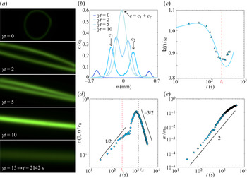
In all cases, a blob of  ${\rm A}$ surrounded by B is initially bordered by a more or less faint fluorescent contour of F singling-out the smeared region between the reactants. The blob then progressively tilts and stretches, bringing its two close-to-parallel borders nearby in the contracting direction
 $n$ under the effect of the shear. At some point these product lamellae merge to form a single lamella with increased concentration, which dilutes by pure diffusion at a later time (figure 2).
(a) Laminar shear of a blob of A in a solution of B ( $Da = 6$). (b) Averaged concentration profiles along the flow (
 $x$-direction). (c) Normalized width of the product thickness profile
 $\mathfrak {b}(t)/s_0$ vs time; the blue line is the expectation from (3.5). (d) Normalized product F maximal concentration
 $c(0,t)/c_0$ vs time, and scaling from (3.8). (e) Normalized net product formed
 $m/m_0$ vs time.

The three limit production regimes identified above ((3.8), (3.10) for  $Da>1$ and (3.14) for
 $Da<1$) are observed.
4.1. $Da>1$

We start with a blob whose contour has been appreciably smeared during injection ( $s_0=0.1$ mm), sheared at a rate
 $\gamma = 7 \times 10^{-3}\ {\rm s}^{-1}$ such that
 $Da=6$ (figure 2). Its initial diameter is
 $d = 1.2$ mm. The solutions have a viscosity of
 $\eta = 2\ {\rm Pa}\ {\rm s}$, yielding
 $k=4.7 \times 10^{-2}\ {\rm mol}^{-1}\ {\rm l}\ {\rm s}^{-1}$. The
 ${\rm B}$ concentration
 $c_{B0}=3 \times 10^{-1}\ {\rm mol} \ {\rm l}^{-1}$ corresponds to a reaction time
 $t_c=40$ s. The Péclet numbers and mixing times are
 $Pe_d = 1028$,
 $t_d = 1413$ s,
 $Pe = 7.2$ and
 $t_s=270$ s.
Within one lamella, the constant flux regime  $c(0,t)\sim c_0 \sqrt {Dt}/s_0$ in (3.8) is clearly visible at a short time before
 $t=t_s$ as well as, during the same time interval, the decay of the transverse width of the product concentration profile
 $\mathfrak {b}(t)$.
Then the increase of  $c(0,t)$ slows down, before a surge in
 $t=t_d$, which corresponds to the fusion of the adjacent lamellae on both sides of the deformed blob (figure 2). In this large Damköhler number limit, chemical production is slaved at molecular mixing, and when the entire blob of A has mixed in B for
 $t>t_d$, the reaction is finished. Beyond that time, the product decays as a passive scalar would do, that is, as
 $c(0,t)\sim (t/t_d)^{-3/2}$ as is well known in this simple shear configuration (Souzy et al. Reference Souzy, Zaier, Lhuissier, Le Borgne and Metzger2018).
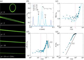
Another similar experiment shown in figure 3 with a blob more sharply defined ( $s_0=0.044$ mm) with
 $Da=10$ (the corresponding parameters are
 $\gamma = 7 \times 10^{-2}\ {\rm s}^{-1}$,
 $\eta = 10^{-1}\ {\rm Pa}\ {\rm s}$,
 $k=1.1\ {\rm mol}^{-1}\ {\rm l}\ {\rm s}^{-1}$,
 $c_{B0}=6 \times 10^{-1}\ {\rm mol}\ {\rm l}^{-1}$,
 $t_c=2$ s,
 $Pe = 3.5$,
 $t_s=21$ s,
 $d=0.6$ mm,
 $Pe_d=682$ and
 $t_d=123$ s) exhibits this time the constant maximal concentration
 $c(0,t)\sim c_0/2$ expected in this regime (
 $Da>1$) when the initial interface irregularity
 $s_0$ is rapidly absorbed. This regime prevails as long as the adjacent lamellae merge in
 $t=t_d$, adding up their concentration profiles. The operation is indeed an addition since the linearity (in
 $c$) of the Fourier-Ranz equation in (3.6) indicates that if
 $c_1(\xi,\tau )$ and
 $c_2(\xi,\tau )$ are the concentration profiles of the first and second lamella on each side of the blob, both ruled by (3.6), then
 \begin{equation} c(\xi,\tau) = c_1(\xi,\tau) + c_2(\xi,\tau) \end{equation}
is also ruled by the same equation. Close to the blob mixing time, when the distance between its borders in the contracting direction  $\sim d/\sqrt {1+(\gamma t)^2}$ becomes smaller than the diffusion width of the product profile
 $\mathfrak {b}(t_d)$, the product diffusion profiles overlap through a linear superposition. This operation, which is at the root of the self-convolution route of mixtures evolution (Villermaux Reference Villermaux2019), has already been witnessed in pure scalar decay (Duplat & Villermaux Reference Duplat and Villermaux2008; Souzy et al. Reference Souzy, Zaier, Lhuissier, Le Borgne and Metzger2018); it is here exemplified by the presence of the reaction since the concentrations in each lamellae, instead of decaying as they add up, are growing (figure 3).
(a) Laminar shear of a blob of A in a solution of B ( $Da =10$). (b) Averaged concentration profiles along the flow (
 $x$-direction). (c) Normalized width of the product thickness profile
 $\mathfrak {b}(t)/s_0$ vs time; the blue line is the expectation from (3.5). (d) Normalized product F maximal concentration
 $c(0,t)/c_0$ vs time. (e) Normalized net product formed
 $m/m_0$ vs time.

4.2. $Da< 1$

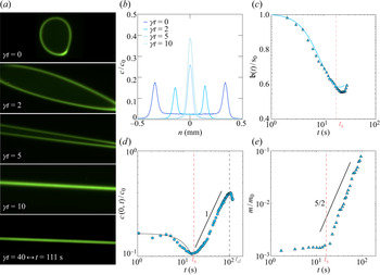
We were able to produce an experiment where the product formation is slightly more controlled by chemistry than by diffusion at  $Da = 0.85$, with appreciable initial smearing. The parameters are as follows:
 $s_0=0.077$ mm,
 $\gamma = 3.6 \times 10^{-1}\ {\rm s}^{-1}$,
 $\eta = 2\ {\rm Pa}\ {\rm s}$,
 $k=4.7 \times 10^{-2}\ {\rm mol}^{-1}\ {\rm l}\ {\rm s}^{-1}$,
 $c_{B0}=6 \times 10^{-1}\ {\rm mol}\ {\rm l}^{-1}$,
 $t_c=20$ s,
 $Pe = 211$,
 $t_s=17$ s,
 $d=1.28$ mm,
 $Pe_d=58\,514$ and
 $t_d=109$ s.
The product F formed during the preparation stage mixes, when shear is set in, as a passive scalar would do precisely because, in this limit,  $t_s< t_c$ (figure 4c,d). The maximal concentration of F decays up to the mixing time
 $t_s$ as
 $c(0,t< t_s)=c_0/\sqrt {1+4\tau (t)}$. Then, the chemical reaction produces F according to (3.14), with a characteristic linear temporal increase.
(a) Laminar shear of a blob of A in a solution of B ( $Da = 0.85$). (b) Averaged concentration profiles along the flow (
 $x$-direction). (c) Normalized width of the product thickness profile
 $\mathfrak {b}(t)/s_0$ vs time; the blue line is the expectation from (3.5). (d) Normalized product F maximal concentration
 $c(0,t)/c_0$ vs time, and scaling from (3.14). (e) Normalized net product formed
 $m/m_0$ vs time.

4.3. Net production
It is customary to underline the benefit of substrate stirring by computing the net ‘mass’ of product  $m$ at time
 $t$ (see e.g. Bandopadhyay et al. Reference Bandopadhyay, Le Borgne, Méheust and Dentz2017). For a blob of
 ${\rm A}$ with surface
 $\sim d^2$ reacting in a medium of
 ${\rm B}$ as it elongates with length
 $\ell (t)\sim d\sqrt {1+(\gamma t)^2}$, we have when
 $Da>1$
 \begin{equation} m\sim\int_0^t\ell(t') j(t') \,{\rm d}t', \end{equation}
where the reactants’ flux  $j(t)$ depends on the Batchelor scale
 $\mathfrak {b}(t)$ given in (3.5). Depending on the interface thickness
 $s_0$ and associated mixing time
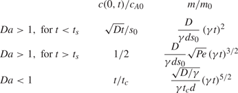
 $t_s$, the two regimes identified in (3.8) and (3.10) are listed in table 1. When
 $Da<1$ (see (3.14)), the net product formed per lamella length
 $\sim c_{A0}\sqrt {Dt}\times t/t_c$ extended to the interface length
 $\ell (t)\sim d \,\gamma t$ provides the corresponding expression in table 1. In all cases,
 $m$, normalized by
 $m_0=d^2c_{A0}$ in figures 2, 3 and 4 above, is a strong function of the blob elongation
 $\gamma t$, confirming the anticipated enhancement of chemical production by substrate stirring.
Summary of the different regimes explored, and associated temporal dependences. The net mass  $m$ is normalized by
 $m_0=d^2c_{A0}$.

5. Conclusion
We have illustrated by experiments in a simple shear flow the interplay between chemical reaction and substrate deformation, and adapted Ranz's formulation for scalar mixing to the case of a reactive mixture between initially segregated reactants A and B. Instead of treating explicitly the chemical cross-term  $kc_Ac_B$, we have globalized it as a production term involving a flux
 $j(t)$ imposed by the rate at which the reaction zone is fed by the reactants, a formulation valid in the large Damköhler number limit (
 $Da>1$ in § 3.1). When
 $Da<1$, the reactants interpenetrate before they react, giving rise to a ‘diffusio-chemical’ regime where chemical production occurs within a substrate whose width is controlled by molecular diffusion. Guilbert & Villermaux (Reference Guilbert and Villermaux2021) have shown how the latter regime induces the rectification of the product composition in a randomly stirred mixture.
Declaration of interests
The authors report no conflict of interest.