1. Introduction
Bubbly flows are usually employed in industry when the rate of mass transfer between a gas and a liquid is limited by the diffusion of the solute in the liquid. They combine the advantages of a large interfacial area by unit of volume and of an intense liquid agitation, which enhances the mixing of solute and accelerates chemical reactions. In many applications, the gas volume fraction
 ${\it\alpha}$
is larger than 20 % and locally reaches much larger values. Bubbles can thus not be considered as isolated and collective effects have to be accounted for.
A first major collective effect is the decrease of the average bubble rise velocity
 $\langle V_{z}\rangle$
when increasing the gas volume fraction. The prediction of the increase of the bubble drag is an important issue for industrial applications. In the literature, several experimental works have investigated this phenomenon. Among them, the experiments of Wallis (Reference Wallis1961), who investigated a homogenous bubble swarm of air bubbles in a soapy water solution, suggest that the rise velocity scales as
 $\langle V_{z}\rangle \propto (1-{\it\alpha})$
up to a gas volume fraction of 30 %. This scaling law was established by considering the global conservation of the mass of gas, where the gas flow rate was measured directly and the gas volume fraction was deduced from the variation of the hydrostatic pressure. Using the same procedure and making an analogy with a fluidized bed, Bridge, Lapidus & Elgin (Reference Bridge, Lapidus and Elgin1964) found a rather similar scaling,
 $\langle V_{z}\rangle \propto (1-{\it\alpha})^{1.39}$
, for the case of a countercurrent liquid flow, with air sparged into water, glycerine/water or water/isoamyl–alcohol mixtures, for
 ${\it\alpha}\leqslant 20\,\%$
. Wijngaarden & Kapteijn (Reference Wijngaarden and Kapteijn1990) determined the mean relative velocity of air bubbles in water by means of a technique based on electric conductance measurements and found that it scaled as
 $(1{-}1.78{\it\alpha})$
up to a gas volume fraction of 14 %. In the presence of a liquid flow Garnier, Lance & Marié (Reference Garnier, Lance and Marié2002) observed that
 $\langle V_{z}\rangle$
scaled as
 ${\it\alpha}^{1/3}$
for
 ${\it\alpha}\leqslant 40\,\%$
by means of a dual-tip optical probe. For different various two-phase flow configurations, Ishii & Chawla (Reference Ishii and Chawla1979) and Rusche & Issa (Reference Rusche and Issa2000) found more complex expressions. In order to estimate relative velocity in bubbly, droplet or particulate flows, Ishii & Chawla (Reference Ishii and Chawla1979) proposed a model based on an effective viscosity of the two-phase mixture. Rusche & Issa (Reference Rusche and Issa2000) introduced a drag correction as a combination of a power law and an exponential function with coefficients that depend on the nature of the considered dispersed flow. Direct numerical simulations of a swarm of bubbles rising in a periodic domain have also been performed. For moderate Reynolds number (
 $\mathit{Re}=O(10{-}100)$
), using a front tracking method and avoiding bubble coalescence, the decrease of
 $\langle V_{z}\rangle$
with
 ${\it\alpha}$
has been confirmed for both spherical (Bunner & Tryggvason Reference Bunner and Tryggvason2002a
,Reference Bunner and Tryggvason
b
) and ellipsoidal bubbles (Bunner & Tryggvason Reference Bunner and Tryggvason2003). Deformed bubbles at large Reynolds number (
 $\mathit{Re}=O(100{-}1000)$
) for
 ${\it\alpha}\leqslant 45\,\%$
have been simulated by Roghair et al. (Reference Roghair, Lau, Deen, Slagter, Baltussen, Van Sint Annaland and Kuipers2011) who used 20 Eulerian mesh points on the surface of each bubble. They observed that the decrease of the bubble velocity was affected by the bubble Eötvös number as well as by the value of the gas volume fraction. Despite the great number of experimental and numerical attempts, no general model for the rise velocity of bubbles exists yet, owing to the complexity of bubbly flows. Experimental investigations at large gas volume fractions (
 ${\it\alpha}>15\,\%$
) with accurate determination of both the bubble geometry and velocity are thus still desirable.
A second collective effect of great significance is the modification of the interfacial rate of mass transfer when the gas volume fraction is increased. Despite the significant gas volume fractions that are present in most industrial applications, many studies make use of mass transfer models developed for isolated bubbles. These models are usually based on Higbie’s penetration theory (Higbie Reference Higbie1935), but consider various definitions for the contact time: (i) the ratio of the bubble diameter to the bubble rise velocity; (ii) the ratio of the bubble surface to the rate of surface formation (Nedeltchev, Jordan & Schumpe Reference Nedeltchev, Jordan and Schumpe2006); or (iii) based on the eddy velocity for developed turbulent flows (Lamont & Scott Reference Lamont and Scott1970; Kawase, Halard & Moo-Young Reference Kawase, Halard and Moo-Young1987; Linek et al.
Reference Linek, Kordac, Fujasova and Moucha2004). With a contact time defined as the ratio of the bubble diameter to the bubble rise velocity (i), the Higbie’s penetration theory is also known as the Boussinesq solution (Boussinesq Reference Boussinesq1905). Numerical simulations (Takemura & Yabe Reference Takemura and Yabe1998; Figueroa & Legendre Reference Figueroa and Legendre2010) have shown that this analytical solution appears to be very accurate at describing interfacial mass transfer for a single clean spherical bubble rising in a still liquid, at large bubble Reynolds and Péclet numbers. Moreover, the experiments by Alves, Vasconcelos & Orvalho (Reference Alves, Vasconcelos and Orvalho2006) showed that this solution was still valid for the interfacial mass transfer of a single bubble fixed in a turbulent downward liquid flow, up to a certain dissipation rate of the turbulence. The Boussinesq solution has also been used as a closure law in Eulerian–Eulerian two-fluid simulations of industrial ozonation towers (Cockx et al.
Reference Cockx, Do-Quang, Liné and Roustan1999) and aeration tanks for urban wastewater treatment (Fayolle et al.
Reference Fayolle, Cockx, Gillot, Roustan and Heduit2007) at low to moderate volume fractions (
 ${\it\alpha}\leqslant 10\,\%$
). Higbie’s penetration theory with a contact time based on the rate of surface formation (ii) has been found to provide a good estimate of the mass transfer rate in a pressurized bubble column for either water or organic liquids (Nedeltchev, Jordan & Schumpe Reference Nedeltchev, Jordan and Schumpe2007). In the same time, Higbie’s penetration theory with a contact time defined with eddy velocity (iii) has been preferred by Buffo, Vanni & Marchisio (Reference Buffo, Vanni and Marchisio2012) and Petitti et al. (Reference Petitti, Vanni, Marchisio, Buffo and Podenzani2013) to simulate gas–liquid mass transfer in stirred tank reactors.
As indicated above, Boussinesq solution is a priori limited to large bubble Reynolds and Péclet numbers and isolated spherical bubbles. Some corrections based on results for a single bubble have been introduced to account for the effect of finite Reynolds number (Darmana, Deen & Kuipers Reference Darmana, Deen and Kuipers2005; Ayed, Chahed & Roig Reference Ayed, Chahed and Roig2007; Shimada, Tomiyama & Ozaki Reference Shimada, Tomiyama and Ozaki2007) and that of bubble deformation (Nedeltchev et al. Reference Nedeltchev, Jordan and Schumpe2007) in simulations of bubble columns. Such corrections are discussed by Takemura & Yabe (Reference Takemura and Yabe1998) and Figueroa & Legendre (Reference Figueroa and Legendre2010). Reviews for mass transfer can be found in Clift, Grace & Weber (Reference Clift, Grace and Weber1978) and in Michaelides (Reference Michaelides2006) for bubbles, but also for drops and particles. Most of these studies have focused on mass or heat transfer from a single inclusion. Their applicability in dense dispersed flow is an important issue.
In the last few decades, a few works have focused on collective effect upon mass transfer in a bubble swarm (Koynov & Khinast Reference Koynov and Khinast2005; Kishore, Chhabra & Eswaran Reference Kishore, Chhabra and Eswaran2008; Colombet et al. Reference Colombet, Legendre, Cockx, Guiraud, Risso, Daniel and Galinat2011; Roghair Reference Roghair2012). Most of them are numerical works. Two-dimensional numerical simulations of mass transfer for different arrangements of bubbles have been performed by Koynov & Khinast (Reference Koynov and Khinast2005) for small Reynolds numbers. For the case of three bubbles initially aligned horizontally, the authors observed a decrease of the Sherwood number. For this particular case, they noticed that, taking into account the reduced Reynolds number, the Sherwood number stays close to that of a single bubble. They also found a decrease of the Sherwood number for the case of bubbles which were initially aligned in the vertical direction. According to Koynov & Khinast (Reference Koynov and Khinast2005), this is due to the fact that bubbles are rising in the wake of each other so that both the gradient of concentration and the interfacial mass flux are reduced. One of their conclusions is that ‘Mass transfer in a bubble swarm depends both on the motion of the swarm as a whole and on the motion of the individual bubbles and, in general, does not follow trends observed in the single bubble cases’. For both Newtonian and non-Newtonian fluids, Kishore et al. (Reference Kishore, Chhabra and Eswaran2008) used a ‘cell model’ of two concentric spheres to study numerically the collective effect of mass transfer for a clean spherical bubble. In that simplified approach, the increase of gas volume fraction is modelled by a decrease of the bounding sphere. The results seem to suggest an increase of the Sherwood number with the increase of the gas volume fraction.
The effect of increasing the gas volume fraction on the gas–liquid mass transfer coefficient has been experimentally investigated by Colombet et al. (Reference Colombet, Legendre, Cockx, Guiraud, Risso, Daniel and Galinat2011) for air bubbles in water. Thanks to a high-speed camera with a fixed focal lens, a particle tracking velocimetry (PTV) method was able to measure bubble volumes, shapes and velocities for gas volume fractions from 0.45 to 16.5 %. In this range, the mass transfer coefficient is found very close to that of a single bubble provided that the Reynolds number is based on the mean equivalent diameter and the average rising velocity of a bubble in the swarm, which suggests a weak influence of the collective effect on the mass transfer at high Péclet number. In a recent study using direct numerical simulation, Roghair (Reference Roghair2012) found a marginal increase of the mass transfer coefficient
 $k_{L}$
with the increase of the gas volume fraction for 4 mm air bubbles rising in water at
 $\mathit{Re}\leqslant 1070,~\mathit{Sc}=1$
and
 $4\leqslant {\it\alpha}\leqslant 40\,\%$
.
The objective of the present study is to investigate collective effect on the bubble dynamics and mass transfer in very dense homogeneous bubbly flows with controlled hydrodynamic conditions. For this purpose, accurate measurements of interfacial area, bubble diameter, deformation and rising velocity are first performed for
 $12.1\leqslant {\it\alpha}\leqslant 33.9\,\%$
. Then, oxygen mass transfer experiments are conducted for
 $0.7\leqslant {\it\alpha}\leqslant 29.6\,\%$
. The paper is organized as follows. Section 2 describes the experimental methods. Section 3 presents the dynamics of the bubbles while § 4 shows the results concerning mass transfer. Section 5 is devoted to the analysis and the discussion of the results. Section 6 summarizes the main conclusions.
2. Experimental set-up and instrumentation
2.1. General description
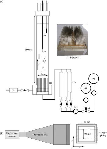
The experimental set-up is described in figure 1(a). It has been used previously by Riboux, Risso & Legendre (Reference Riboux, Risso and Legendre2010) and Colombet et al. (Reference Colombet, Legendre, Cockx, Guiraud, Risso, Daniel and Galinat2011). Bubbles are injected through stainless steel capillaries (1) in a square glass column of
 $15~\text{cm}\times 15~\text{cm}$
cross-section and 100 cm high. The gas line is equipped with three different rotameters (2) and one manometer (3) to deal with a large range of gas flow rates and volume fractions. A three-way valve enables the switch from nitrogen to air (4). The use of 841 capillaries of 15 cm length and
 $d_{c}=0.2~\text{mm}$
inner diameter ensures an homogeneous injection of bubbles of almost equal sizes.
(a) Experimental installation and (b) imaging set-up.

Experiments are performed at ambient temperature and pressure (
 $T=20\,^{\circ }\text{C}$
and
 $P=P_{atm}$
). The liquid used for all experiments is tap water filtered to remove particles larger than
 $15~{\rm\mu}\text{m}$
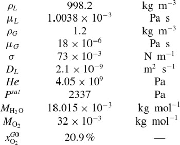
(5). As a consequence, in the regime considered, gas–liquid interfaces can be considered to be clean (Ellingsen & Risso Reference Ellingsen and Risso2001). This point has been carefully validated by measuring the terminal velocity for single bubbles. The main physical properties of the system are summarized in table 1.
System properties at
 $T=20\,^{\circ }\text{C}$
and
 $P=101\,325~\text{Pa}$
.

2.2. Measurements of gas volume fraction and bubble velocity
The gas volume fraction
 ${\it\alpha}$
and the average vertical bubble velocity
 $\langle V_{z}\rangle$
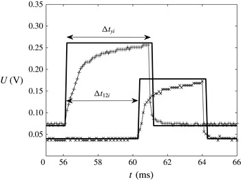
are measured by means of a dual-tip optical fibre probe (RBI Instrumentation) which is introduced at the centre of the column (7). A threshold just higher than the noise level is first applied on the raw signal to define the binarized signal. An example of raw and binarized signals obtained for each fibre is presented in figure 2. Then, the volume fraction is determined from
 $$\begin{eqnarray}{\it\alpha}=\frac{\sum {\rm\Delta}t_{yi}}{t_{aqc}},\end{eqnarray}$$
where
 $t_{acq}$
is the acquisition duration,
 ${\rm\Delta}t_{yi}$
the residence time of bubble
 $i$
on the first fibre (see figure 2) and
 ${\it\Sigma}{\rm\Delta}t_{yi}$
the total time during which the gas phase is detected. The signal acquisition is performed with a sampling frequency of 10 kHz. A good statistical convergence and an overall accuracy better than 2 % is obtained for a recording time larger than 800 s.
Signals from the optical probe. Symbols: raw signal from first (
 $+$
) and second (
 $\times$
) fibre. Line: binarized signals (——).

The vertical velocity
 $V_{zi}$
of bubble
 $i$
is obtained by
 $$\begin{eqnarray}V_{zi}=\frac{d_{s}}{{\rm\Delta}t_{12i}},\end{eqnarray}$$
where
 ${\rm\Delta}t_{12i}$
is the time elapsed between the detection of the bubble interface by the first and the second fibre (as reported in figure 2) and
 $d_{s}$
is the distance between the two fibre tips. The main difficulty of this technique is to match two successive rising fronts corresponding to the piercing of the same bubble. Spurious unrealistic low or large velocity measurements are detected in some cases, especially when two bubbles interact close to the probe. According to the sensitivity study of Riboux (Reference Riboux2007), values smaller than
 $V_{min}=0.03~\text{m}~\text{s}^{-1}$
or larger than
 $V_{max}=0.7~\text{m}~\text{s}^{-1}$
have been removed.
2.3. Measurement of bubble geometrical characteristics
The most reliable technique to determine the bubble shape is probably to process images obtained by means of a high-speed camera. A classic way to image the bubbles is to use a fixed focal lens with a thin depth of field, as done by Colombet et al. (Reference Colombet, Legendre, Cockx, Guiraud, Risso, Daniel and Galinat2011). However, the larger the gas volume fraction, the more numerous are blurred out-of-focus bubbles in the field of view. The use of a fixed focal lens is thus limited to moderate gas volume fractions (
 ${\it\alpha}\leqslant 15\,\%$
).
The study of collective effects in a dense bubble swarm therefore requires the development and the use of another optical technique. In the present work, we use a telecentric lens, which has the particularity to have a depth of field larger than the column width (15 cm) and a constant magnification factor all along the direction of view. The main advantage is to image bubbles with sharp contours, even in a very dense bubbly flow. The main drawback is that the increase of the field of view results in a significant reduction of the spatial resolution. In addition, it has been possible to follow individual bubbles only on a short distance. For those two reasons, the measurement of the bubble velocity is less accurate and image processing has been specifically used to measure the bubble geometrical characteristics.
The imaging set-up consists of a high-speed CMOS camera (Photron APX, figure 1
b) equipped with a telecentric lens (TC-4M-172 Opto Engineering) to visualize a window of
 $94~\text{mm}\times 94~\text{mm}$
located at the centre of the column at a distance of 150 mm above the injectors tips. The spacial resolution is
 $5.8~\text{pixel}~\text{mm}^{-1}$
. The camera is operated at 500 images per second with an exposure time varying from
 $1/20\,000$
to
 $1/500~\text{s}$
depending on the lighting intensity. Lighting is supplied by an halogen spot of 1000 W.
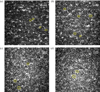
The recorded images are processed by using Matlab®. The bubble edges are detected by applying a threshold to the raw images in grey levels. The interior of the bubbles is then filled and small aberrant objects detected in the picture are removed. A test of convexity is performed to identify cases for which the detected object corresponds to two superimposed bubbles. It consists of comparing the surface area
 $S_{obj}$
of the detected object to the area
 $S_{conv}$
of the smallest convex polygon that can contain the object. Only the objects with
 $S_{obj}/S_{conv}\geqslant 0.95$
are retained, the others being discarded. Examples of detected contours are drawn on typical raw images in figure 3 for different gas volume fractions.
Typical images of the bubble swarm with detected bubble contours marked with yellow/light lines: (a)
 ${\it\alpha}=12.2\,\%$
; (b)
 ${\it\alpha}=23.9\,\%$
; (c)
 ${\it\alpha}=30.6\,\%$
; (d)
 ${\it\alpha}=33.9\,\%$
.

The geometrical properties of the bubbles are determined by assuming that the bubbles are oblate spheroids with a minor semi-axis
 $a$
and a major semi-axis
 $b$
, which are measured from the two-dimensional measured contours. The bubble aspect ratio is defined as
 ${\it\chi}=b/a$
. The bubble volume is estimated from
 $V_{b}=4{\rm\pi}b^{2}a/3$
and its equivalent diameter from
 $$\begin{eqnarray}d=(8b^{2}a)^{1/3}.\end{eqnarray}$$
The bubble area
 $S_{b}$
is estimated by (Beyer Reference Beyer1987)
 $$\begin{eqnarray}S_{b}={\rm\pi}\frac{d^{2}}{4}\left(2{\it\chi}^{2/3}+\frac{{\it\chi}^{-4/3}}{\sqrt{1-{\it\chi}^{-2}}}\ln \left(\frac{1+\sqrt{1-{\it\chi}^{-2}}}{1-\sqrt{1-{\it\chi}^{-2}}}\right)\right).\end{eqnarray}$$
In addition, an indirect determination of the bubble equivalent diameter can be obtained from the dual-tip optical probe by assuming that all of the bubbles have the same size. As recalled by Colombet (Reference Colombet2012), for a monodispersed population of bubbles that impact the probe with null angle of attack,
 $d$
can be expressed as a function of the average chord length
 $\langle y\rangle$
,
 $$\begin{eqnarray}d={\textstyle \frac{3}{2}}\langle y\rangle {\it\chi}^{2/3},\end{eqnarray}$$
where
 $\langle y\rangle$
is obtained from optical probe measurements as
 $$\begin{eqnarray}\langle y\rangle =\frac{\mathop{\sum }_{1}^{n}(V_{zi}{\rm\Delta}t_{yi})}{n},\end{eqnarray}$$
and
 ${\it\chi}$
from image processing. (Note that the size distribution of the bubbles will be discussed in § 3.1 from the results of image processing.)
2.4. Measurement of interfacial area
For a bubble column of total volume
 $V_{tot}$
, the volumetric interfacial area,
 $a_{I}=\sum S_{b}/V_{tot}$
, is related to the gas volume fraction,
 ${\it\alpha}=\sum V_{b}/V_{tot}$
, by the relation
 $$\begin{eqnarray}a_{I}={\it\alpha}\frac{\sum S_{b}}{\sum V_{b}}.\end{eqnarray}$$
As indicated above, for each bubble detected,
 $a$
and
 $b$
are obtained from the images used to determine the bubble volume
 $V_{b}$
and surface
 $S_{b}$
. The volume fraction
 ${\it\alpha}$
is given by the optical probe. Then, the interfacial area
 $a_{I}$
is determined by using (2.7).
2.5. Measurement of mass transfer
The concentration
 $C(z,t)$
of oxygen dissolved in water at time
 $t$
and elevation
 $z$
is measured by means of fast response probes: Clark-type microsensors (Unisense Ox50). The technique is based on the measurement of the intensity of the electric current between an anode and an oxygen-reducing cathode, which is proportional to the oxygen concentration. Calibration of oxygen probes is performed for each experiment. Since the probe response is linear on the whole range of concentration considered, a calibration is performed in situ by using the signal measured at the beginning (anoxic water) and the end (saturated water) of each experiment. The relative uncertainty on oxygen concentration measurements is
 $\pm 2\,\%$
. In the present configuration, as shown in figure 1(6), two oxygen probes have been placed at two different elevations
 $z$
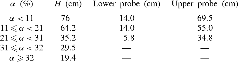
, which are reported in table 2.
Liquid height
 $H$
at
 ${\it\alpha}=0$
and elevation of the oxygen probes above capillaries tips.

As shown in Colombet et al. (Reference Colombet, Legendre, Cockx, Guiraud, Risso, Daniel and Galinat2011), due to the moderate height of the bubble column (
 ${\leqslant}70~\text{cm}$
), the oxygen saturation concentration in the water is almost unaffected by the variation of hydrostatic pressure (6.4 %) or by the depletion of the oxygen concentration within the bubbles during the mass transfer (6 %). Moreover, the dilution of oxygen in the bubbles induced by liquid-to-gas transfer of nitrogen at the beginning of the experiments can also be neglected (1.3 %). Consequently, the oxygen mass saturation concentration
 $C^{\ast }$
can be considered as constant along the
 $z$
axis and equal to its value at the upper surface where the pressure is equal to that of the atmosphere (
 $P=P_{atm}$
), so that
 $$\begin{eqnarray}C^{\ast }=x_{\text{O}_{2}}^{G0}{\it\rho}_{\text{H}_{2}\text{O}}\frac{M_{\text{O}_{2}}}{M_{\text{H}_{2}\text{O}}}\frac{(P-P^{sat})}{\mathit{He}}\approx 9.08~\text{mg}~\text{l}^{-1},\end{eqnarray}$$
with
 $x_{\text{O}_{2}}^{G0}$
the molar fraction of oxygen in the gas phase (dry air),
 ${\it\rho}_{\text{H}_{2}\text{O}}={\it\rho}_{L}$
the density of water (
 $\text{kg}~\text{m}^{-3}$
),
 $M$
the molar masses (
 $\text{kg}~\text{mol}^{-1}$
),
 $P^{sat}$
the vapour pressure of water in the bubbles (Pa) and
 $\mathit{He}$
the Henry constant for oxygen in water (Pa). Equation (2.8) results from Henry’s law for oxygen in water and Raoult’s law for water in air with activity and fugacity coefficients equal to unity for both equilibria, assuming that the liquid is essentially composed of water.
The classical ‘gassing-out’ method is used to determine the time scale of the transfer of oxygen from the bubbles to the water. This method consists in first bubbling nitrogen gas in the column in order to remove the oxygen that is initially naturally present in water. Next, without changing the inlet gas flow rate in order to not disturb the dynamics of the bubble swarm, air is suddenly injected instead of nitrogen. The concentration of dissolved oxygen
 $C$
then increases until it reaches the saturation concentration
 $C^{\ast }$
.
The moderate size of the column and the bubble-induced turbulence both contribute to an efficient liquid mixing so that the liquid phase can be assumed to be perfectly mixed for each horizontal slice of the bubble column. Moreover, owing to the large gas volume fractions and interfacial areas considered in this work, the vertical mass flux of dissolved oxygen generated by the axial mixing can be neglected compared with the oxygen flux coming from the bubbles. In such conditions, the variation of the concentration of dissolved oxygen along the bubble column is given by
 $$\begin{eqnarray}\frac{\partial C(z,t)}{\partial t}=\frac{k_{L}\,a_{I}}{(1-{\it\alpha})}(C^{\ast }-C(z,t)),\end{eqnarray}$$
where
 $k_{L}$
is the liquid-side mass transfer coefficient and
 $a_{I}$
the interfacial area. In the present configuration, the only reason for which
 $C$
depends on
 $z$
comes from the delay corresponding for the time taken by the bubble to reach a given elevation
 $z$
. In the following the time origin is shifted by
 $z/\langle V_{z}\rangle$
so that the concentration no more depends on
 $z$
and the signals provided by the two oxygen probes are synchronized.
The analysis of the measured concentrations requires to account for the response time
 ${\it\tau}_{p}$
of the probes (Letzel et al.
Reference Letzel, Schouten, Krishna and van den Bleek1999; Martin, Montes & Galan Reference Martin, Montes and Galan2007). For this purpose, the oxygen probe is assumed to behave as a first-order system
 $$\begin{eqnarray}\frac{\partial C_{p}}{\partial t}=(1/{\it\tau}_{p})(C-C_{p}),\end{eqnarray}$$
where
 $C$
is the real concentration and
 $C_{p}$
is the value provided by the probe. The response time of each probe has been measured and found close to
 ${\it\tau}_{p}=0.8~\text{s}$
. Solving (2.10) and (2.9) for a sudden increase of the mass concentration from 0 to
 $C^{\ast }$
at
 $t=0$
, it yields
 $$\begin{eqnarray}\frac{C_{p}}{C^{\ast }}=1-\frac{1}{({\it\tau}-{\it\tau}_{p})}({\it\tau}\text{e}^{-t/{\it\tau}}-{\it\tau}_{p}\text{e}^{-t/{\it\tau}_{p}}),\end{eqnarray}$$
where the time scale
 ${\it\tau}$
is related to the mass transfer coefficient
 $k_{L}$
by
 $$\begin{eqnarray}{\it\tau}=\frac{(1-{\it\alpha})}{k_{L}a_{I}}.\end{eqnarray}$$
2.6. Homogeneity of the bubble swarm
Our purpose is to study a stable bubble column in which there is no gradient of volume fraction and no large-scale liquid motions induced by buoyancy. The use of an array of capillary tubes guarantees that the bubbles are uniformly injected at the bottom of the column. However, increasing the gas volume fraction may lead to the development of an instability and to the transition to a churn flow. The onset of the instability depends on both the liquid height
 $H$
in the column and the gas volume fraction. For
 $H=70~\text{cm}$
, the flow is stable up to approximately
 ${\it\alpha}=10\,\%$
. For larger values of
 ${\it\alpha}$
, the liquid height has been reduced in order to keep a stable flow. The chosen values of
 $H$
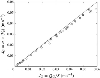
are reported in table 2. With this choice, the free surface at the top of the column remains still and the gas volume fraction turns out to be uniform all over the column. Figure 4 compares the superficial gas velocity
 $J_{G}={\it\alpha}\times \langle V_{z}\rangle$
obtained from
 $\langle V_{z}\rangle$
and
 ${\it\alpha}$
measured by the optical probe and the superficial gas velocity
 $J_{G}=Q_{G}/S$
obtained from a gas flow rate
 $Q_{G}$
measured from the flowmeters. The good agreement obtained between these two estimations for all gas volume fractions investigated (
 $0.45\leqslant {\it\alpha}\leqslant 33.9\,\%$
) confirms the homogeneity of the gas distribution over the column.
Superficial gas velocity from gas volume fraction and bubble average rising velocity measured by the dual-tip optical probe
 $J_{G}={\it\alpha}\times \langle V_{z}\rangle$
versus superficial gas velocity from measured gas flow rate
 $J_{G}=Q_{G}/S$
.

Another departure to the flow homogeneity may come from the fact that the bubbles need a certain distance to reach their terminal velocity and that mass transfer needs a certain time to attain a steady state. Considering a clean spherical bubble starting from rest, the relaxation time scale of the bubble velocity can be estimated by
 ${\it\tau}_{V}\approx d^{2}/(72{\it\nu}_{L})\approx 0.06~\text{s}$
, which corresponds to a distance
 $3{\it\tau}_{V}V_{z}\approx 5.4~\text{cm}$
. Concerning the mass transfer, Figueroa & Legendre (Reference Figueroa and Legendre2010) found a transient time
 ${\it\tau}_{C}\approx 10(d^{3}{\it\chi}/8)^{1/3}/V_{z}$
for
 $\mathit{Re}=300$
,
 $\mathit{Sc}=10$
and
 ${\it\chi}=1.2$
. In our case, this leads to
 ${\it\tau}_{C}\approx 0.04~\text{s}$
and
 ${\it\tau}_{C}V_{z}\approx 1.3~\text{cm}$
. It is therefore reasonable to consider that the flow and the mass transfer are fully developed at the location of the first oxygen probes, which is at least 5.8 cm above the capillaries.
3. Characterization of the bubble dynamics
In this section, the bubble dynamics is characterized in terms of bubble size, velocity, deformation, interfacial area and relevant dimensionless numbers. The results obtained by means of a telecentric lens are systematically presented together with those of Colombet et al. (Reference Colombet, Legendre, Cockx, Guiraud, Risso, Daniel and Galinat2011), who used a fixed focal lens in the same experimental set-up for
 $0.45\leqslant {\it\alpha}\leqslant 16.5\,\%$
. In figures 5–7, 9(b) and 10(a), the errorbars indicate the uncertainty related to the image resolution on the measurement of bubble size and to the measurement of
 ${\it\alpha}$
. In figures 9(a), 10(b) and 11, errorbars indicate the uncertainty related to the measurement of
 $\langle d\rangle$
by considering an uncertainty of
 $\pm 0.02~\text{m}~\text{s}^{-1}$
on the determination of the average bubble velocity
 $\langle V_{z}\rangle$
.
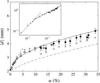
Average bubble equivalent diameter as a function of the gas volume fraction: ●, image processing with a telecentric lens; ○, image processing with a fixed focal lens by Colombet et al. (Reference Colombet, Legendre, Cockx, Guiraud, Risso, Daniel and Galinat2011);
 $\times$
, dual-tip optical probe measurements from average bubble chords (2.5); – – –, (3.1); ——, (3.2); – ⋅ – ⋅ –, dynamic bubble formation model of Gaddis & Vogelpohl (Reference Gaddis and Vogelpohl1986). Inset: log–log representation of
 $(\langle d\rangle -d_{0})/d_{0}$
versus
 ${\it\alpha}$
.

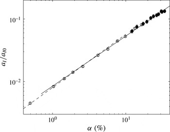
Interfacial area (2.7) versus gas volume fraction: ●, this work; ○, from Colombet et al. (Reference Colombet, Legendre, Cockx, Guiraud, Risso, Daniel and Galinat2011); – – –, (3.3); ——, (3.4).

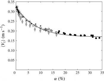
Average bubble velocity against the gas volume fraction. Dual-tip optical probe measurements from this work (●), Colombet et al. (Reference Colombet, Legendre, Cockx, Guiraud, Risso, Daniel and Galinat2011) (○), Riboux et al. (Reference Riboux, Risso and Legendre2010) (*). PTV by image processing from Colombet et al. (Reference Colombet, Legendre, Cockx, Guiraud, Risso, Daniel and Galinat2011) (▫); ——, (3.5).

3.1. Equivalent diameter and interfacial area
Figure 5 shows the evolution of the average bubble equivalent diameter
 $\langle d\rangle$
measured from image processing (2.3) as a function of
 ${\it\alpha}$
(○, ●). The standard deviation of the equivalent diameter measured by image processing is found to range between 11 and 21 % of the average value. The bubbles are therefore almost monodisperse and (2.5) can also be used to estimate the bubble diameter from optical probe signals. The values determined by this method are also plotted in figure 5 (
 $\times$
). Despite the strong assumptions made, including that the probe is considered to be ideal (Kiambi et al.
Reference Kiambi, Duquenne, Bascoul and Delmas2001; Vejrazka et al.
Reference Vejrazka, Sechet, Vecer, Orvalho, Ruzicka and Cartellier2010) and that all of the bubbles impact the probe with a null angle of attack, the difference between the two experimental techniques is less than 14 %.
The bubble diameter is observed to increase with
 ${\it\alpha}$
because of the process of bubble formation and detachment from the capillaries. At a very low gas volume fraction, the bubble formation can be considered as quasi-static and the bubble size is controlled by the equilibrium between buoyancy and capillary forces at the tip of the capillaries. The diameter is then given by the Tate law,
 $d_{T}=[6{\it\sigma}d_{c}/({\rm\Delta}{\it\rho}g)]^{1/3}=2.07~\text{mm}$
, as confirmed by the measurement of the detachment of a single bubble by Riboux et al. (Reference Riboux, Risso and Legendre2010). When increasing the inlet gas velocity
 $u_{c}$
, the balance of the forces acting on a bubble involves drag and added-mass forces (Gaddis & Vogelpohl Reference Gaddis and Vogelpohl1986; Duhar & Colin Reference Duhar and Colin2006). For the entire range of gas volume fraction considered here, the Weber number based on the capillary inner diameter,
 $\mathit{We}_{c}={\it\rho}_{L}u_{c}^{2}d_{c}/{\it\sigma}$
, stays much lower than two so that the jet regime is never reached and the bubble generation corresponds either to the static regime of formation or to the dynamic one (Mersmann Reference Mersmann1977). Knowing the gas flow rate through each capillary, the bubble diameter can be estimated by using the model of Gaddis & Vogelpohl (Reference Gaddis and Vogelpohl1986). The predictions of this model, which are reported in figure 5, show the same trend as the experimental results but with an underestimation of approximately 20 %. This discrepancy can be due to a collective effect of the bubbles on the formation process and to bubble coalescence that may take place just above the capillary tip as observed by Manasseh, Riboux & Risso (Reference Manasseh, Riboux and Risso2008).
A log–log representation (see the inset in figure 5) reveals that the evolution of
 $\langle d\rangle$
is well described by the succession of two power laws:
 $$\begin{eqnarray}\displaystyle & \displaystyle \frac{\langle d\rangle -d_{0}}{d_{0}}\approx 15{\it\alpha}\quad \text{for }{\it\alpha}\leqslant 2.3\,\% & \displaystyle\end{eqnarray}$$
 $$\begin{eqnarray}\displaystyle & \displaystyle \frac{\langle d\rangle -d_{0}}{d_{0}}\approx 2.3{\it\alpha}^{0.5}\quad \text{for }{\it\alpha}>2.3\,\% & \displaystyle\end{eqnarray}$$
 $d_{0}=2.1~\text{mm}$
is the value for a single bubble detaching in the static regime from one capillary (
 ${\it\alpha}=0$
).
Figure 6 shows the evolution of the interfacial area as a function of the gas volume fraction. It is found to regularly increase with
 ${\it\alpha}$
according to the following empirical power laws
 $$\begin{eqnarray}\displaystyle & \displaystyle \frac{a_{I}}{a_{I0}}\approx 0.402{\it\alpha}^{0.85}\,\quad \text{for }{\it\alpha}\leqslant 2.3\,\% & \displaystyle\end{eqnarray}$$
 $$\begin{eqnarray}\displaystyle & \displaystyle \frac{a_{I}}{a_{I0}}\approx 0.336{\it\alpha}^{0.8}\,\quad \text{for }{\it\alpha}>2.3\,\% & \displaystyle\end{eqnarray}$$
 $a_{I0}=S_{b0}/V_{b0}=3011~\text{m}^{-1}$
is the surface-to-volume ratio of a single bubble detaching in the static regime.
3.2. Bubble velocity
3.2.1. Average velocity
During the last decade, many works have investigated the velocity of bubbles rising in a swarm (Rusche & Issa Reference Rusche and Issa2000; Zenit, Koch & Sangani Reference Zenit, Koch and Sangani2001; Garnier et al. Reference Garnier, Lance and Marié2002; Riboux et al. Reference Riboux, Risso and Legendre2010). All of these studies report a significant decrease of the average bubble vertical velocity as the gas volume fraction increases.
Figure 7 shows the average vertical bubble velocity
 $\langle V_{z}\rangle$
as a function of
 ${\it\alpha}$
. The present results obtained with a dual optical probe (●) are compared with those of Riboux et al. (Reference Riboux, Risso and Legendre2010) (*) and Colombet et al. (Reference Colombet, Legendre, Cockx, Guiraud, Risso, Daniel and Galinat2011) (○) that were obtained with the same technique, and to those of Colombet et al. (Reference Colombet, Legendre, Cockx, Guiraud, Risso, Daniel and Galinat2011) (▫) that were determined by image processing with a fixed focal lens. The velocity obtained from image processing is slightly lower, probably because the detected bubbles are not far enough from the column wall. However, all of the results obtained with an optical probe collapse onto a master curve of equation
 $$\begin{eqnarray}\langle V_{z}\rangle =V_{z0}\left[0.28+0.72\exp (-15{\it\alpha})\right]^{0.5}\!,\end{eqnarray}$$
where
 $V_{z0}=0.32~\text{m}~\text{s}^{-1}$
is the rise velocity of an isolated bubble formed on a single capillary in the quasi-static bubbling regime, measured by Riboux et al. (Reference Riboux, Risso and Legendre2010). It is remarkable that a single simple correlation is able to describe the evolution of the average bubble velocity on a such large range of gas volume fraction (
 $0.45\leqslant {\it\alpha}\leqslant 29.6\,\%$
) along which
 $\langle V_{z}\rangle$
is reduced by almost a factor of two (from 0.32 to
 $0.17~\text{m s}^{-1}$
).
It is important to stress that all empirical relations relating the properties of the gas phase to the gas volume fraction that have been introduced above ((3.1)–(3.5), (4.1), (4.3) and (4.5)) may depend on the particular system of gas injection used here and are therefore not universal. However, they will be of great interest to analyse and discuss the results of the present work in the following.
3.2.2. Velocity fluctuations
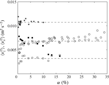
Figure 8 shows the variances of the bubble velocity fluctuations. Let us first discuss the variance of the velocity signal provided by the dual optical probe from this work (○) for
 ${\it\alpha}$
up to 30 % and from Riboux et al. (Reference Riboux, Risso and Legendre2010) (*) for
 ${\it\alpha}$
up to 12 %. As noted by Riboux et al. (Reference Riboux, Risso and Legendre2010), if the dual optical probe is an accurate technique to measure the average vertical bubble velocity, it does not provide a reliable value of the variance of the bubble vertical velocity. The reason comes from the fact that the considered bubbles are oblate spheroid which move with oscillating velocity and orientation. The fluctuations that are recorded by the dual probe are thus a complex combination of the fluctuations of the vertical velocity, orientation and shape. For that reason, the measured variance is observed to depend on the exact probe geometry. The values obtained by Riboux et al. (Reference Riboux, Risso and Legendre2010) with a distance between the two fibre tips of 0.5 mm is indeed significantly larger than that obtained in the present work with a fibre tip separation of 1 mm. However, the variance provided by the dual optical probe can be used to characterize the evolution with the gas volume fraction of the overall energy of agitation of the bubbles in the vertical direction. It was already noticed that the bubble vertical agitation keeps a constant value up to a gas volume fraction of around 10 % by Martínez-Mercado, Palacios-Morales & Zenit (Reference Martínez-Mercado, Palacios-Morales and Zenit2007) and Riboux et al. (Reference Riboux, Risso and Legendre2010), which suggested that the energy of bubble agitation remains controlled by wake instabilities. The present results seem to show that this result holds up to
 ${\it\alpha}=30\,\%$
.
Variances of bubble velocity against gas volume fraction. Variance obtained from the dual optical probe in this work (○) and by Riboux et al. (Reference Riboux, Risso and Legendre2010) (*). Variances of the vertical velocity (▫) and the horizontal velocity (▪) measured in this work from particle tracking on images taken with a fixed focal lens.

(a) Bubble Reynolds number (
 $\mathit{Re}=\langle V_{z}\rangle \langle d\rangle /{\it\nu}_{L}$
) and (b) Eötvös number (
 $\mathit{Eo}={\rm\Delta}{\it\rho}g\,\langle d\rangle ^{2}/{\it\sigma}$
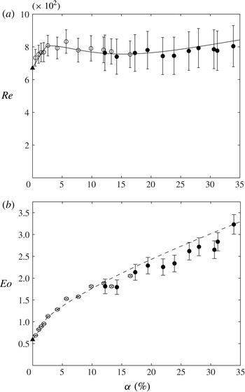
) versus gas volume fraction: ○, method using a fixed focal lens; ●, method using a telecentric lens; ▴, result for a single bubble from Riboux et al. (Reference Riboux, Risso and Legendre2010); ——, Reynolds number determined form fitted data ((3.1), (3.2) and (3.5)); – – –, Eötvös number determined form fitted data ((3.1) and (3.2)).

(a) Bubble average aspect ratio and (b) Weber number (
 $\mathit{We}={\it\rho}_{L}\langle V_{z}\rangle ^{2}\langle d\rangle /{\it\sigma}$
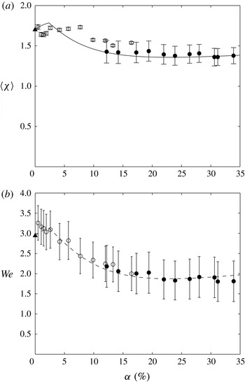
) versus gas volume fraction: ○, method using a fixed focal lens; ●, method using a telecentric lens; ▴, result for a single bubble from Riboux et al. (Reference Riboux, Risso and Legendre2010); ——, aspect ratio estimated from (3.6) (Legendre, Zenit & Velez-Cordero Reference Legendre, Zenit and Velez-Cordero2012); – – –, Weber number determined form fitted data ((3.1), (3.2) and (3.5)).

In order to have a more complete description of the bubble agitation, we have also determined the velocity variance of the horizontal and the vertical bubble velocity fluctuations by PTV based on images taken with a fixed focal lens. As stated before, this imaging technique already used by Colombet et al. (Reference Colombet, Legendre, Cockx, Guiraud, Risso, Daniel and Galinat2011) is limited to moderate volume fractions. The corresponding results are also plotted in figure 8 for
 ${\it\alpha}$
up to 16 %. Both the horizontal and the vertical variances are found to be almost constant,
 $\langle {v_{z}^{\prime }}^{2}\rangle \approx 0.003~\text{m}^{2}~\text{s}^{-2}$
and
 $\langle {v_{x}^{\prime }}^{2}\rangle \approx 0.0075~\text{m}^{2}~\text{s}^{-2}$
, for
 ${\it\alpha}$
up to 10 %. As shown by Ellingsen & Risso (Reference Ellingsen and Risso2001), the horizontal component of the fluctuant velocity of an isolated bubble evolves as
 $v_{x}^{\prime }={\it\omega}A_{x}\cos ({\it\omega}t)$
. For the present bubble size, Riboux (Reference Riboux2007) measured an angular frequency of
 ${\it\omega}=29~\text{rad}~\text{s}^{-1}$
and a path amplitude
 $A_{x}$
varying from 3.5 to 4.9 mm, which gives a variance
 $\langle {v_{x}^{\prime }}^{2}\rangle =(A_{x}{\it\omega})^{2}/2$
from 0.005 to
 $0.01~\text{m}^{2}~\text{s}^{-2}$
, in agreement with the values found here at moderate volume fraction. When
 ${\it\alpha}$
is increased beyond 10 %, the vertical variance remains constant, while the horizontal one decreases down to match the vertical value around
 ${\it\alpha}=12\,\%$
. Such a decrease of the horizontal fluctuation of the dispersed phase has already been reported in a solid/liquid fluidized bed by Aguilar Corona (Reference Aguilar Corona2008) and Aguilar Corona, Zenit & Masbernat (Reference Aguilar Corona, Zenit and Masbernat2011). It may result from hindrance effects on bubble paths when increasing
 ${\it\alpha}$
.
3.3. Bubble Reynolds, Eötvös and Weber numbers
In order to fully characterize the present flow regime, it is useful to consider the values taken by the relevant dimensionless numbers in the range of volume fractions investigated. These values can be computed either from the raw values of the measured dimensional quantities or from the empirical fits proposed in the previous sections. In the following figures, plots systematically represent raw data whereas lines corresponds to values obtained from fitted data.
Figure 9(a) shows the Reynolds number,
 $\mathit{Re}=\langle V_{z}\rangle \langle d\rangle /{\it\nu}_{L}$
. It first increases from 670 to 780 as
 ${\it\alpha}$
increases from 0 to 2.5 % and then keeps a constant value as
 ${\it\alpha}$
is further increased. The constance of the Reynolds number for
 ${\it\alpha}\geqslant 2.5\,\%$
results from the fact that the increase in the bubble diameter (figure 5) is compensated by the decrease of the rise velocity (figure 7). A similar result was observed for a volume fraction up to 10 % by Martínez-Mercado et al. (Reference Martínez-Mercado, Palacios-Morales and Zenit2007), who also used a bank of capillaries to inject the bubbles. This is an interesting property of this type of experimental set-up, which allows the volume fraction to be varied while keeping the Reynolds number constant.
Figure 9(b) shows the Eötvös number:
 $\mathit{Eo}={\rm\Delta}{\it\rho}g\langle d\rangle ^{2}/{\it\sigma}$
. As expected from the evolution of
 $\langle d\rangle$
, it regularly increases from 0.5 to 3.2 as
 ${\it\alpha}$
varies from 0 to 30 %.
Figure 10(a) presents the mean bubble aspect ratio,
 $\langle {\it\chi}\rangle$
, which is found to slightly decrease from 1.7 to 1.4. The bubble deformation is known to be controlled by both the Weber number (Moore Reference Moore1965) and the Morton number (Legendre et al.
Reference Legendre, Zenit and Velez-Cordero2012). Here, since we are considering a single system of fluids with constant physical properties, the Morton number is constant:
 $\mathit{Mo}=g{\it\nu}_{L}^{4}{\it\rho}_{L}^{2}{\rm\Delta}{\it\rho}/{\it\sigma}^{3}=2.5\times 10^{-11}$
. The measured Weber number,
 $\mathit{We}={\it\rho}_{L}\langle V_{z}\rangle ^{2}\langle d\rangle /{\it\sigma}$
, is plotted in figure 10(b). It is found to decrease from approximately 3.25 down to 1.8. Since the Reynolds number is almost constant, the Weber number turns out to be proportional to
 $\langle V_{z}\rangle$
. The decrease of the average aspect ratio, by approximately 30 %, is of the same order as that of
 $\mathit{We}$
, and both
 $\langle {\it\chi}\rangle$
and
 $\mathit{We}$
keep an almost constant value for
 ${\it\alpha}>15\,\%$
. These results are in good agreement, within 14 %, with the relation proposed by Legendre et al. (Reference Legendre, Zenit and Velez-Cordero2012) for a single bubble at low Morton number:
 $$\begin{eqnarray}{\it\chi}=\frac{1}{1-{\textstyle \frac{9}{64}}\,\mathit{We}}.\end{eqnarray}$$
3.4. Collective effect on bubble drag coefficient
We consider now the evolution of the bubble drag coefficient
 $C_{d}$
with the gas volume fraction in order to analyse the collective effect of the bubbles on their rise velocity. Here
 $C_{d}$
is determined from the balance between drag and buoyancy forces as
 $$\begin{eqnarray}C_{d}=\frac{4}{3}\,\frac{{\rm\Delta}{\it\rho}}{{\it\rho}_{L}}\frac{g\langle d\rangle }{\langle V_{z}\rangle ^{2}},\end{eqnarray}$$
where
 $g$
is the acceleration of gravity, the average equivalent diameter
 $\langle d\rangle$
is measured from image processing and the average rise velocity
 $\langle V_{z}\rangle$
from the dual-tip optical probe. The experimental results are shown in figure 11 (○, ●) as a function of the gas volume fraction. Here
 $C_{d}$
is observed to increase from 0.26 for
 ${\it\alpha}=0.45\,\%$
and
 $\langle d\rangle \approx 2.5~\text{mm}$
to 2.4 at
 ${\it\alpha}=34\,\%$
and
 $\langle d\rangle \approx 5~\text{mm}$
.
Experimental drag coefficient (3.7) against gas volume fraction:

 $\cdots \cdots$
, Garnier et al. (Reference Garnier, Lance and Marié2002) (3.11); – – –, Roghair et al. (Reference Roghair, Lau, Deen, Slagter, Baltussen, Van Sint Annaland and Kuipers2011) (3.12).

In order to disentangle the effect of the bubble size to that of the gas volume fraction, it is interesting to compare the present results with those obtained for single rising bubbles of the same diameter. The drag coefficient
 $C_{d_{0}}$
of a deformed single bubble at terminal velocity is commonly estimated by (Tomiyama et al.
Reference Tomiyama, Kataoka, Zun and Sakaguchi1998)
 $$\begin{eqnarray}C_{d_{0}}=\frac{8}{3}\,\frac{\mathit{Eo}}{c_{1}+c_{2}\,\mathit{Eo}},\end{eqnarray}$$
with
 $c_{1}=4$
and
 $c_{2}=1$
according to Mendelson (Reference Mendelson1967),
 $c_{1}=4.28$
and
 $c_{2}=1.02$
according to Comolet (Reference Comolet1979) and
 $c_{1}=19/3$
and
 $c_{2}=2/3$
for
 $\mathit{Re}>600$
with air/water systems according to Dijkhuizen et al. (Reference Dijkhuizen, Roghair, Van Sint Annaland and Kuipers2010).
The corresponding values are represented by empty squares and triangles in figure 11. Starting from similar values at low gas volume fractions,
 $C_{d}$
and
 $C_{d_{0}}$
quickly diverge as
 ${\it\alpha}$
increases. In the present experiments, the increase of
 $C_{d}$
turns out to mainly result from hydrodynamic bubble interactions. The collective effect of bubbles is really important and leads to a drag coefficient 2.4 times larger than that of an isolated bubble at
 ${\it\alpha}=34\,\%$
.
In the literature devoted to bubbly flows, numerous relations have been proposed to describe the evolution of the drag coefficient with the gas volume fraction. Considering air bubbles injected through a porous sparger in a column of 9.5 cm diameter filled with a soapy water solution, Wallis (Reference Wallis1961) proposed the following correlation, for
 $3<{\it\alpha}<30\,\%$
 $$\begin{eqnarray}C_{d}=C_{d_{0}}(1-{\it\alpha})^{-2},\end{eqnarray}$$
which was later used for one-dimensional gas–liquid modelling (Wallis Reference Wallis1969, p. 52). We have computed
 $C_{d}$
using relation (3.9) with
 $C_{d_{0}}$
from Mendelson (Reference Mendelson1967). The corresponding values are represented by a plain line in figure 11. They are in fairly good agreement with the present measurements.
Applying a mixture viscosity model to their experimental results, Ishii & Chawla (Reference Ishii and Chawla1979) (see also Ishii & Zuber Reference Ishii and Zuber1979) found the following correction to account for the effect of the gas volume fraction on the bubble drag coefficient:
 $$\begin{eqnarray}C_{d}=\frac{C_{d_{0}}}{(1-{\it\alpha})}\left(\frac{1+17.67\,[f({\it\alpha})]^{6/7}}{18.67\,f({\it\alpha})}\right)^{2}\quad \text{with }f({\it\alpha})=(1-{\it\alpha})^{1.5}.\end{eqnarray}$$
This relation is also reported in figure 11 (dashed-dotted line) by using the expression proposed by Mendelson (Reference Mendelson1967) for
 $C_{d_{0}}$
. It predicts an evolution of
 $C_{d}$
that is close to that of Wallis (Reference Wallis1961) so that it is difficult to conclude which is in best agreement with the present results.
Garnier et al. (Reference Garnier, Lance and Marié2002) experimentally investigated a homogeneous air/water bubbly flow in the presence of a co-current liquid flow for volume fractions up to 30 % and Reynolds numbers from 300 to 500. They results led to
 $$\begin{eqnarray}C_{d}=C_{d_{0}}\left(1-{\it\alpha}^{1/3}\right)^{-2}.\end{eqnarray}$$
Using again the expression proposed by Mendelson (Reference Mendelson1967) for
 $C_{d_{0}}$
, this relation (dotted line in figure 11) is found to considerably over-predict the effect of the gas volume fraction upon the drag coefficient compared with the present results.
Roghair et al. (Reference Roghair, Lau, Deen, Slagter, Baltussen, Van Sint Annaland and Kuipers2011) performed numerical simulations of a bubble swarm in a periodic cubic domain for
 $1\leqslant \mathit{Eo}\leqslant 5$
,
 $4\times 10^{-12}\leqslant \mathit{Mo}\leqslant 2\times 10^{-9}$
and
 ${\it\alpha}\leqslant 45\,\%$
. From their results, they proposed the following relation
 $$\begin{eqnarray}C_{d}=C_{d_{0}}\left(1+\frac{18}{\mathit{Eo}}{\it\alpha}\right),\end{eqnarray}$$
where
 $C_{d_{0}}$
is given by the relation proposed by Dijkhuizen et al. (Reference Dijkhuizen, Roghair, Van Sint Annaland and Kuipers2010). This relation suggests that the collective effect of the bubbles on the drag coefficient may depend on other parameters than the gas volume fraction, such as the Eötvös number. The corresponding values of
 $C_{d}$
are represented by a dashed line in figure 11. They are approximately 30 % higher than the present experimental data, just at the limit of the measurement uncertainty.
4. Mass transfer
In this section, the measured mass transfer coefficients and Sherwood numbers are first presented as a function of the gas volume fraction. Then, they are compared with available correlations for a single bubble rising in a liquid at rest. Finally, they are compared with transfer rates expected in a highly turbulent flow. In figures 14 and 15, errorbars indicate the uncertainty related to the measurement of the interfacial area
 $a_{I}$
, the gas volume fraction
 ${\it\alpha}$
, the bubble equivalent diameter
 $\langle d\rangle$
by considering an uncertainty of
 $\pm 10\,\%\,{\it\tau}$
on the determination of the mass transfer time scale
 ${\it\tau}$
.
4.1. Experimental results
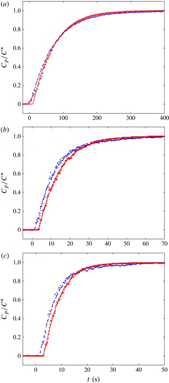
The time evolutions of the oxygen concentration are presented in figure 12 for
 ${\it\alpha}=1.46\,\%$
(a),
 ${\it\alpha}=15.1\,\%$
(b) and
 ${\it\alpha}=26.9\,\%$
(c). In this figure, the time origin has not been shifted by
 $z/\langle V_{z}\rangle$
so that the signal of the upper probe is delayed compared with the first. The least-squares method is used to fit each set of experimental data by (2.11) in order to obtain the transfer time scale
 ${\it\tau}$
. The corresponding fitting curves, represented by lines in figure 12, describe accurately the experimental results, confirming that the assumptions made about the probe response and the fact that the flow is well mixed are fulfilled.
Typical measured time evolutions of the concentration of dissolved oxygen of (a)
 ${\it\alpha}=1.46\,\%$
, (b)
 ${\it\alpha}=15.1\,\%$
and (c)
 ${\it\alpha}=26.9\,\%$
: ●, lower probe; ○ upper probe; – – – and ——, (2.11).

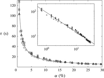
A total of 38 experimental runs have been conducted in the range of
 $0.7\leqslant {\it\alpha}\leqslant 29.6\,\%$
. The corresponding values of
 ${\it\tau}$
are reported in figure 13 together with the 29 values measured by Colombet et al. (Reference Colombet, Legendre, Cockx, Guiraud, Risso, Daniel and Galinat2011) in the range
 $0.45\leqslant {\it\alpha}\leqslant 16.5\,\%$
. The time necessary to reach the saturation is significantly affected by the void fraction since it decreases by more than one order of magnitude between
 ${\it\alpha}=1\,\%$
and
 ${\it\alpha}=30\,\%$
. Such a strong decrease is expected from the strong increase of the interfacial area with
 ${\it\alpha}$
(figure 6). As it is clearly visible in the log–log plot proposed in the inset of figure 13, the experimental values of
 ${\it\tau}$
nicely follow a simple power law,
 $$\begin{eqnarray}{\it\tau}\approx {\it\tau}_{0}\,{\it\alpha}^{-0.8}\quad \text{with}~{\it\tau}_{0}=2.22~\text{s}.\end{eqnarray}$$
Time scale of the mass transfer versus the gas volume fraction: ▫, lower probe; ▵, upper probe; ○, Colombet et al. (Reference Colombet, Legendre, Cockx, Guiraud, Risso, Daniel and Galinat2011) (using a single oxygen probe); ——, experimental fit (4.1). Inset: log–log representation.

In order to analyse the collective effect of the bubbles on the mass transfer, we have to consider the mass transfer coefficient by unit of area,
 $k_{L}$
. The experimental value of
 $k_{L}$
is obtained from the measured values of
 ${\it\tau}$
,
 ${\it\alpha}$
and
 $a_{I}$
by
 $$\begin{eqnarray}k_{L}=\frac{(1-{\it\alpha})}{{\it\tau}\,a_{I}}.\end{eqnarray}$$
Combining relations (3.4) for
 $a_{I}$
and (4.1) for
 ${\it\tau}$
, the following simple empirical relation is found for the mass transfer coefficient, for
 ${\it\alpha}>2.3\,\%$
 $$\begin{eqnarray}k_{L}\approx k_{L_{0}}(1-{\it\alpha})\quad \text{with}~k_{L_{0}}=4.45\times 10^{-4}~\text{m s}^{-1}.\end{eqnarray}$$
Figure 14(a) shows the evolution of the experimental values of
 $k_{L}$
as a function of the gas volume fraction. The decrease is considerably lower compared with that of
 ${\it\tau}$
, which indicates that most of the evolution of the total rate of transfer results from the trivial effect of the augmentation of the interfacial area and justifies the efforts made to obtain an accurate determination of
 $a_{I}$
.
Mass transfer coefficient (a) and Sherwood number (b) versus gas volume fraction. Experiments: ▫, this work (average values); ○, Colombet et al. (Reference Colombet, Legendre, Cockx, Guiraud, Risso, Daniel and Galinat2011);

 $\cdots \cdots$
, (4.8) (Winnikow Reference Winnikow1967); – – –, (4.9) (Takemura & Yabe Reference Takemura and Yabe1998); ——, (4.10) (Colombet et al.
Reference Colombet, Legendre, Cockx and Guiraud2013);
——, (4.12) and (4.13) (Figueroa & Legendre Reference Figueroa and Legendre2010).

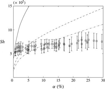
Comparison of the measured Sherwood number with mass transfer models for turbulent flows. Present experiments: same legend as in figure 14; (4.14) and (4.15) with ——
 $c_{1}=2/\sqrt{{\rm\pi}}$
(Kawase et al.
Reference Kawase, Halard and Moo-Young1987), – – –
 $c_{1}=0.523$
(Linek et al.
Reference Linek, Kordac, Fujasova and Moucha2004), — ⋅ —
 $c_{1}=0.4$
(Lamont & Scott Reference Lamont and Scott1970).

To go further in the analysis of the physical mechanism underlying the mass transfer, we have to make dimensionless the rate of mass transfer by introducing the Sherwood number
 $$\begin{eqnarray}\mathit{Sh}=\frac{k_{L}\left\langle d\right\rangle }{D_{L}},\end{eqnarray}$$
where
 $D_{L}$
is the diffusion coefficient of dissolved oxygen in water. Figure 14(b) shows the evolution of the experimental Sherwood number as a function of
 ${\it\alpha}$
, which using empirical fits (3.1), (3.2), (4.3) and (4.4) can be described by the following empirical relation, for
 ${\it\alpha}>2.3\,\%$
 $$\begin{eqnarray}\mathit{Sh}\approx \mathit{Sh}_{0}(1-{\it\alpha})(1+2.3\,{\it\alpha}^{0.5})\quad \text{with}~\mathit{Sh}_{0}=445.\end{eqnarray}$$
The increase of
 $\langle d\rangle$
almost compensates for the decrease of
 $k_{L}$
so that
 $\mathit{Sh}$
turns out to increase moderately with the gas volume fraction, its values (4.5) remaining between 600 and 750 in the whole range of
 ${\it\alpha}$
investigated.
The present results therefore suggest that the collective effect of the bubbles has a relatively weak influence on the interfacial mass transfer considering the huge effect observed on the transfer time scale
 ${\it\tau}$
. However, it is difficult to conclude from the sole evolution of the Sherwood number since variations of bubble size, velocity and shape are associated with variation of gas volume fractions. In next section, we will compare the present results with those corresponding to a single bubble in the same flow regime and with the same geometrical properties.
4.2. Comparison with a single bubble rising in a liquid at rest
In most studies of mass transfer in bubble columns, the rate of transfer is estimated by using Higbie’s penetration theory (Higbie Reference Higbie1935),
 $$\begin{eqnarray}k_{L}=\frac{2}{\sqrt{{\rm\pi}}}\sqrt{\frac{D_{L}}{t_{c}}},\end{eqnarray}$$
where
 $t_{c}$
is taken equal to
 $\langle d\rangle /\langle V_{z}\rangle$
. In fact this is equivalent to the analytical solution obtained by Boussinesq (Reference Boussinesq1905) by considering that the flow around the bubble can be approximated by the potential flow and a very thin concentration layer on the bubble
 $$\begin{eqnarray}\mathit{Sh}=\frac{2}{\sqrt{{\rm\pi}}}\mathit{Pe}^{1/2},\end{eqnarray}$$
where
 $\mathit{Pe}=\langle d\rangle \langle V_{z}\rangle /D_{L}$
is the Péclet number. This solution is thus valid in the limit of large
 $\mathit{Re}$
and
 $\mathit{Pe}$
.
Various improvements have been proposed to account for the effect of bubble deformation or finite Reynolds number upon the mass transfer from a single bubble. Considering the flow approximation of Moore (Reference Moore1963), Winnikow (Reference Winnikow1967) derived the following expression that includes the effect of the Reynolds number:
 $$\begin{eqnarray}\mathit{Sh}=\frac{2}{\sqrt{{\rm\pi}}}\left[1-\frac{2.89}{\sqrt{\mathit{Re}}}\right]^{1/2}\mathit{Pe}^{1/2}.\end{eqnarray}$$
Measuring the mass transfer of almost spherical millimetre-sized bubbles from volume variations, Takemura & Yabe (Reference Takemura and Yabe1998) proposed the following relation,
 $$\begin{eqnarray}\mathit{Sh}=\frac{2}{\sqrt{{\rm\pi}}}\left[1-\frac{2}{3}\frac{1}{(1+0.09\mathit{Re}^{2/3})^{3/4}}\right]^{1/2}(2.5+\mathit{Pe}^{1/2})\end{eqnarray}$$
which was found to be in good agreement with both experiments and numerical simulations at moderate
 $\mathit{Re}$
numbers and large
 $\mathit{Pe}$
.
Recently, considering numerical results from various previous works, Colombet et al. (Reference Colombet, Legendre, Cockx and Guiraud2013) proposed the following relation that is valid for a spherical bubble whatever the value of
 $\mathit{Re}$
and
 $\mathit{Pe}$
,
 $$\begin{eqnarray}\mathit{Sh}=1+\left[1+\left(\frac{4}{3\,{\rm\pi}}\right)^{2/3}\left(2\,\mathit{Pe}_{max}\right)^{2/3}\right]^{3/4},\end{eqnarray}$$
where
 $\mathit{Pe}_{max}$
is the Péclet number based on the maximal velocity
 $U_{max}$
of the liquid at the interface instead of the bubble velocity
 $V_{z}$
, which is obtained from the correlation proposed by Legendre (Reference Legendre2007),
 $$\begin{eqnarray}\frac{U_{max}}{V_{z}}=\frac{1}{2}\,\frac{16+3.315\mathit{Re}^{1/2}+3\mathit{Re}}{16+3.315\mathit{Re}^{1/2}+\mathit{Re}}.\end{eqnarray}$$
When
 $\mathit{Pe}$
tends to zero, relation (4.10) tends to the diffusive solution in the absence of flow (
 $\mathit{Sh}=2$
) while it tends towards the Boussinesq solution when
 $\mathit{Re}$
and
 $\mathit{Pe}$
become very large.
The effect of the bubble deformation has been studied by Lochiel & Calderbank (Reference Lochiel and Calderbank1964), who considered the potential flow around a spheroidal bubble. They proposed to correct the Boussinesq expression by the introduction of a function
 $f$
of the aspect ratio
 ${\it\chi}$
,
 $$\begin{eqnarray}\mathit{Sh}({\it\chi})=\frac{2}{\sqrt{{\rm\pi}}}\mathit{Pe}^{1/2}f({\it\chi}).\end{eqnarray}$$
The validity of this solution has been recently discussed by Figueroa & Legendre (Reference Figueroa and Legendre2010), who proposed the following expression
 $$\begin{eqnarray}f({\it\chi})=0.524+0.88{\it\chi}-0.49{\it\chi}^{2}+0.086{\it\chi}^{3},\end{eqnarray}$$
which is based on the results of direct numerical simulations, and proved to be valid for
 $500<({\it\chi}/8)^{1/3}\mathit{Re}<1000$
,
 ${\it\nu}_{L}/D_{L}>100$
and
 $1\leqslant {\it\chi}\leqslant 3$
.
The values of
 $k_{L}$
predicted by all of these expressions derived for an isolated bubble are reported in figure 14(a) while the corresponding values of
 $\mathit{Sh}$
are reported in figure 14(b). Because the Reynolds number remains almost constant and the bubble shape does not evolve so much in the present experiments, the predictions of all of these correlations are close to each other. Moreover, these predictions are all in agreement with the experiments, considering the measurement uncertainty.
We can therefore conclude that the mass transfer in a homogeneous bubble swarm at high Péclet number is almost independent of the gas volume fraction. It has been proved to remain similar to that of a single bubble rising in a fluid at rest up to a volume fraction of 30 %. This conclusion is in agreement with the trends of the numerical simulations of Roghair (Reference Roghair2012).
4.3. Comparison with the interfacial transfer in highly turbulent flows
The bubbles generate strong velocity fluctuations in the liquid phase. It is thus interesting to compare the rate of transfer measured here with that induced at a plane interface by a turbulence of similar intensity. It has been shown that turbulent eddies can enhance the mass transfer by causing the renewal of the liquid close to the interface (Magnaudet & Calmet Reference Magnaudet and Calmet2006). Considering that the timescale
 $t_{c}$
of renewal of the liquid at the interface is proportional to
 $({\it\nu}_{L}/\langle {\it\epsilon}_{L}\rangle )^{1/2}$
, where
 ${\it\epsilon}_{L}$
is the rate of dissipation of the turbulence, (4.6) gives
 $$\begin{eqnarray}\mathit{Sh}=c_{1}\left(\frac{d\langle {\it\epsilon}_{L}\rangle ^{1/4}}{{\it\nu}_{L}^{3/4}}\right)\mathit{Sc}^{1/2},\end{eqnarray}$$
where
 $\mathit{Sc}={\it\nu}_{L}/D_{L}$
is the Schmidt number. Several values have been proposed for the prefactor
 $c_{1}$
: 0.4 (Lamont & Scott Reference Lamont and Scott1970), 0.523 (Linek et al.
Reference Linek, Kordac, Fujasova and Moucha2004) or
 $2/\sqrt{{\rm\pi}}$
(Kawase et al.
Reference Kawase, Halard and Moo-Young1987).
In an homogeneous bubbly flow, Riboux et al. (Reference Riboux, Risso and Legendre2010) showed that the rate of dissipation of the energy is given by
 $$\begin{eqnarray}\langle {\it\epsilon}_{L}\rangle \approx \frac{{\rm\Delta}{\it\rho}}{{\it\rho}_{L}}\,{\it\alpha}\langle V_{z}\rangle g.\end{eqnarray}$$
According to (4.15),
 $\langle {\it\epsilon}_{L}\rangle$
ranges from 0.02 to
 $0.5~\text{m}^{2}~\text{s}^{-3}$
for the range of gas volume fraction considered here. The Sherwood numbers given by relation (4.14) are plotted in figure 15. They are clearly not in agreement with the present measurements. Combining (4.15) and (4.14), it yields
 $$\begin{eqnarray}\mathit{Sh}=c_{1}\left(\mathit{Eo}^{3}/\mathit{Mo}\right)^{1/8}{\it\alpha}^{1/4}\mathit{Re}^{1/4}\mathit{Sc}^{1/2}.\end{eqnarray}$$
The evolution of Sherwood number with the gas volume fraction predicted by this relation (
 ${\it\alpha}^{1/4}$
) is not compatible with the experimental result. Moreover, the predicted evolution with the Reynolds number (
 $\mathit{Re}^{1/4}$
) is contradictory to the scaling expected considering the evolution for an isolated bubble (
 $\mathit{Re}^{1/2}$
).
This analysis confirms that the mass transfer in the bubble column is controlled by the mass transfer around a single bubble in fluid at rest. The fact that the liquid agitation may play a negligible role in the mass transfer at a bubble interface has already been noticed by Alves et al. (Reference Alves, Vasconcelos and Orvalho2006), who investigated the case of a single bubble in a turbulent flow with a dissipation rate of one order of magnitude smaller than in the present configuration.
5. Discussion
Hydrodynamic interactions between bubbles have a strong effect on the average bubble rise velocity, which is found to decrease strongly when increasing the gas volume fraction. The analysis of the interactions between two rising bubbles in a liquid at rest reveals opposite effects depending on the relative position of the bubbles. For two bubbles rising in line, the drag force on the trailing bubble is diminished (Yuan & Prosperetti Reference Yuan and Prosperetti1994; Harper Reference Harper1997; Ruzicka Reference Ruzicka2000; Hallez & Legendre Reference Hallez and Legendre2011), so that vertical interactions between bubbles should increase the average bubbles velocity in a bubble swarm. On the other hand, the drag coefficient of two bubbles rising side by side is increased (Legendre, Magnaudet & Mougin Reference Legendre, Magnaudet and Mougin2003; Hallez & Legendre Reference Hallez and Legendre2011), so that transversal interactions between bubbles should decrease the average bubble velocity. In a two-dimensional high-Reynolds-number swarm of bubbles confined between two vertical plates (Bouche et al. Reference Bouche, Roig, Risso and Billet2012), vertical interactions are predominant and both the average and the variance of the vertical bubble velocity is observed to increase with the gas volume fraction. The main difference between this configuration and the present one is that turbulence cannot develop because of the wall friction. In a three-dimensional unconfined bubble swarm, hydrodynamic interactions between bubble wakes cause a strong attenuation of individual wakes (Risso et al. Reference Risso, Roig, Amoura, Riboux and Billet2008). The combination of the wake attenuation with the existence of an intense agitation of both the bubbles and the liquid phase reduces considerably the vertical entrainment by bubbles and explains why the hindering effect is predominant when the gas volume fraction increases. More surprising is the weak influence of hydrodynamic interactions on the variance of the vertical bubble agitation, which is observed to remain close to that of an isolated bubble. Even if bubble path oscillations become erratic, the fluctuant energy of their motion seems still controlled by wake instabilities.
The major finding of the present work is the absence of any significant collective effect of the bubbles on the mass transfer up to volume fraction of 30 %. This result is not valid for any dispersed two-phase flow. Collective effect on the mass transfer are known to exist for a long time (Ranz & Marshall Reference Ranz and Marshall1952). In the 1960s and the 1970s, many experimental works on mass (or heat) transfer in fixed or fluidized bed measured an increase of the Sherwood (or Nusselt) number with the particle volume fraction
 ${\it\alpha}_{S}$
(Ranz & Marshall Reference Ranz and Marshall1952; Rowe & Claxton Reference Rowe and Claxton1965; Littman & Silva Reference Littman and Silva1970; Turner & Otten Reference Turner and Otten1973; Gunn & Souza Reference Gunn and Souza1974; Miyauchi, Kataoka & Kikuchi Reference Miyauchi, Kataoka and Kikuchi1976; Gunn Reference Gunn1978). More recently, numerical simulations have confirmed this trend: Massol (Reference Massol2004) for
 $0\leqslant \mathit{Re}\leqslant 300$
,
 $0.72\leqslant {\it\nu}/D\leqslant 2$
and
 ${\it\alpha}_{S}\leqslant 60\,\%$
; and Deen et al. (Reference Deen, Kriebitzsch, van der Hoef and Kuipers2012) for
 $36\leqslant \mathit{Re}\leqslant 144$
,
 ${\it\nu}/D=0.8$
and
 ${\it\alpha}_{S}=30\,\%$
, who found results in agreement with Gunn (Reference Gunn1978). The point is therefore to understand the absence of collective effect in homogenous bubbly flows.
First, let us discuss the mechanism of mass transfer for a single rising bubble. For large Reynolds and Péclet numbers, Figueroa & Legendre (Reference Figueroa and Legendre2010) showed that the mass transfer mainly takes place across a thin diffusive layer located at the front part of the bubble, where the flow is potential. The thickness
 ${\it\delta}_{D}$
of the concentration boundary layer can be estimated from (Boussinesq Reference Boussinesq1905)
 $$\begin{eqnarray}\frac{{\it\delta}_{D}}{d}\approx \frac{\sqrt{{\rm\pi}}}{2}\mathit{Pe}^{-1/2}.\end{eqnarray}$$
In the present experiments, the Péclet number is around
 $3.5\times 10^{5}$
and
 ${\it\delta}_{D}$
is of the order of
 $10^{-3}\,d$
(
 ${\approx}5~{\rm\mu}\text{m}$
). In order that the solution for a single bubble can apply, two conditions must be fulfilled. First, the average flow in the close surrounding of each bubble have to be similar to that of a isolated bubble. Second, liquid velocity fluctuations must not penetrate within the concentration boundary layer. Experimental investigations of the flow around a bubble immersed within an homogeneous bubble swarm (Risso & Ellingsen Reference Risso and Ellingsen2002; Roig & Larue de Tounemine Reference Roig and Larue de Tounemine2007; Risso et al.
Reference Risso, Roig, Amoura, Riboux and Billet2008) have shown that the first condition is satisfied; in particular, at high bubble Reynolds number, the flow in front of the bubble is well described by the potential solution for a single bubble. The second condition requires that both the distance
 ${\it\delta}_{x}$
between the interfaces of neighbour bubbles and the size of the smallest turbulent eddies
 ${\it\eta}_{K}$
are large compare to the thickness
 ${\it\delta}_{D}$
of the concentration boundary layer.
If bubbles were arranged on a periodic face-centred cubic network, the minimum distance between two bubble interfaces is given by
 $$\begin{eqnarray}\frac{{\it\delta}_{x}}{d}=\left(\frac{1}{\sqrt{2}}\left(\frac{2{\rm\pi}}{3{\it\alpha}}\right)^{1/3}-1\right),\end{eqnarray}$$
which gives
 ${\it\delta}_{x}\approx 0.35\,d\approx 1.6~\text{mm}$
for
 ${\it\alpha}=30\,\%$
.
As suggested by Riboux et al. (Reference Riboux, Risso and Legendre2010), the Kolmogorov microscale of the bubble-induced turbulence, which corresponds to the size of the smallest turbulent eddies, can be roughly estimated by
 $$\begin{eqnarray}{\it\eta}_{K}=\left(\frac{{\it\nu}_{L}^{3}}{\left\langle {\it\epsilon}_{L}\right\rangle }\right)^{1/4},\end{eqnarray}$$
where the average dissipation rate
 $\langle {\it\epsilon}_{L}\rangle$
is determined from (4.15) and gives
 ${\it\eta}_{K}\approx 10^{-2}\,d\approx 50~{\rm\mu}\text{m}$
for
 ${\it\alpha}=30\,\%$
. Both
 ${\it\delta}_{x}$
and
 ${\it\eta}_{K}$
are therefore much larger than
 ${\it\delta}_{D}$
and the second condition is satisfied.
With a Péclet number of 1070, the results of Roghair (Reference Roghair2012) did not show any collective effect. However, in the cases considered by Massol (Reference Massol2004) (
 $\mathit{Pe}=600$
) and Deen et al. (Reference Deen, Kriebitzsch, van der Hoef and Kuipers2012) (
 $\mathit{Pe}=115$
), the mass transfer was observed to depend on the volume fraction of the dispersed phase. This confirms that a large enough Péclet number is necessary so that the mass transfer is not influenced by hydrodynamic interactions.
6. Conclusions
Thanks to an original method of imaging using a telecentric lens and a dual optical probe, the properties of the gas phase have been measured in an homogenous swarm of bubble up to a volume fraction of 30 %. In particular, the bubble deformation is found to be in good agreement with the correlation proposed by Legendre et al. (Reference Legendre, Zenit and Velez-Cordero2012) for a single bubble. Also, the average bubble velocity is observed to strongly decrease with
 ${\it\alpha}$
and found to be in agreement with the correlations of Wallis (Reference Wallis1961) and Ishii & Chawla (Reference Ishii and Chawla1979). Even if some open questions remain concerning the physical mechanism responsible for the increase of the drag coefficient, available correlations are reliable to predict the deformation and the average bubble rise velocity in an homogenous bubble swarm at large Reynolds number. The bubble fluctuating velocity has also been characterized. Surprisingly, no significant influence of the gas volume fraction on the variance measured by means of the dual optical probe was observed. Hydrodynamic interactions between bubbles make the bubble path oscillations irregular, but they do not seem to modify the overall amount of fluctuating energy, which remains controlled by the instability of the wake behind each bubble.
The total mass transfer of oxygen from the bubbles to the liquid has been measured by means of the gassing-out method. Thanks to the determination of the total interfacial area by imaging, the mass transfer rate by unit of area and the Sherwood number have been obtained. Remarkably, the Sherwood number is found to be very close to that of a single bubble rising at the same velocity. The reason lies in the fact that the mass flux occurs in a very thin layer located in front of the bubble. Owing to the large value of the Péclet number (
 ${>}10^{5}$
), the distance between the interfaces of the bubbles and the smallest turbulent eddies are much larger than the thickness of the concentration boundary layer. Consequently, the flow within this layer is not affected by the presence of the other bubbles. Moreover, the mixing generated by the bubble-induced agitation of the liquid ensures that the dissolved oxygen is homogeneous everywhere out of this layer. For the mass transfer the conditions are therefore equivalent to those of a single bubble rising in a fluid at rest and at uniform concentration. Correlations for the Sherwood number established for single rising bubbles are therefore relevant to predict the mass transfer in a homogenous bubble column up to a volume fraction of 30 %, provided that the bubble Reynolds and Péclet numbers are large enough. This conclusion is consistent with the results obtained experimentally for a similar system by Colombet et al. (Reference Colombet, Legendre, Cockx, Guiraud, Risso, Daniel and Galinat2011) for gas volume fractions lower than 17 % and with the numerical simulations of Roghair (Reference Roghair2012) for a Péclet number around 1000. Results obtained at lower Péclet number in fluidized beds however showed an increase of the Sherwood number compared with that of a single particle. There is probably a lower limit below which mass transfer in a dispersed two-phase flow depends on the volume fraction. The determination of this limit, which probably depends on parameters such as the nature of the dispersed phase or the Reynolds number, requires further investigations.
Acknowledgements
The authors would like to thank Rhodia, member of the SOLVAY Group, for supporting this work and especially Dr C. Daniel and Dr S. Galinat. We also thank Sébastien Cazin for their invaluable help on image processing and Grégory Ehses for his help in adapting the experimental set-up for this study. This research was carried out within the framework of a CIFRE-ANRT contract in collaboration with the FERMaT federation.