The question of how much to invest in education—and the returns to those investments—has attracted a great deal of attention in economics (Coleman et al. Reference Coleman1966; Card and Krueger Reference Card and Krueger1992; Betts Reference Betts1996; Hanushek Reference Hanushek1986, Reference Hanushek1996). Publicly funded education has long been viewed as the most important policy tool for improving the future labor market outcomes of children, particularly for youths from disadvantaged backgrounds. Accordingly, concerns about disparities in access to educational resources have motivated a complex and evolving system of transfers from the federal and state governments to local districts.Footnote 1 However, for much of American history, local governments assumed the bulk of the responsibility for financing their own school systems and deciding on spending levels (Stoddard Reference Stoddard2009).
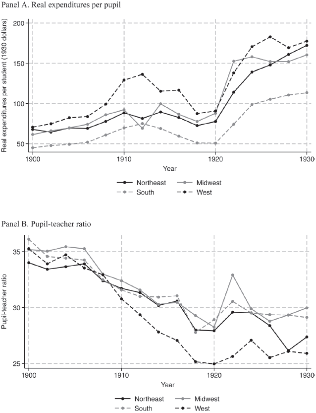
We study the impact of the unprecedented investments in public education made by city school districts in the aftermath of WWI and provide the first nationwide, district-level analysis of spending on education in early twentieth-century America. We digitized reports of education published biennially for city school districts—the finest geographic unit for which there are comprehensive surviving records from this period—from 1900 to 1930 for major cities in the United States from the Report of the Commissioner of Education (1900–1916) and the Biennial Survey of Education (1918–1930). Panel A of Figure 1 displays the trend in real expenditures per pupil in our sample of cities separately by census region. The growth in educational spending by cities after WWI marked a significant departure from nineteenth-century levels. On the eve of the United States entering WWI (1916), real expenditures per pupil were about $84 (in 1930 dollars). However, between 1920 and 1924, expenditures ballooned from $79 to $143 per pupil, an 80 percent increase. Such a rapid increase in real expenditures per pupil would not occur again until the 1960s.
TRENDS IN RESOURCES PER PUPIL FOR SAMPLE CITIES (1900–1930)
Notes: Data are weighted averages in each census region for our sample of 340 cities. In Panel A, the data are weighted by the number of pupils in average daily attendance in each city in every academic year. In Panel B, the data are weighted by the number of teachers in each city in every academic year. Expenditures per pupil are the sum of expenditures on teachers, supervisors, capital, and other expenditures divided by the average daily attendance in a city school system. Real expenditures per student are adjusted using the CPI from Officer and Williamson (Reference Officer and Williamson2021). The year of each data point corresponds to the calendar year in which the academic year ended (e.g., expenditures per pupil for the 1905–1906 academic year are plotted in 1906). The 1914–1915 academic year is plotted in 1916, since we could not find data for the 1915–1916 academic year.
Source: Schmick and Shertzer (Reference Schmick and Shertzer2025).

To obtain adult outcomes for students educated in urban schools during these decades, we matched school-age individuals from the 1910 and 1920 complete count censuses to the 1940 complete count census. Because the 1940 census contains information only on state of birth, linking individuals is essential to match adults in 1940 to the city-level school resources they experienced as children. An advantage of our approach is that we can investigate the potentially heterogeneous returns to educational resources based on childhood socioeconomic status, a task that is generally not possible with retrospective analyses.
Our empirical strategy relies on the observation that post-WWI expansions in school resources were in part a response to immigrants from enemy nations who had already settled in the United States. WWI abruptly downgraded the status of ethnic Germans living in the United States, with lasting effects throughout the 1920s (Moser Reference Moser2012; Ferrara and Fishback Reference Ferrara and Fishback2022). Anti-German hysteria exploded across many facets of American life, from outright violence to politically divisive Americanization laws, some of which outright forbid instruction in the German language (Lleras-Muney and Shertzer Reference Lleras-Muney and Shertzer2015; Fouka Reference Fouka2020). City governments reacted with panic to large populations of German descent and undertook efforts to assimilate the children of enemy aliens through public schooling, along with expanded city school budgets (Ross Reference Ross1994). We argue that anti-German panic can be used to construct an instrument for school resources in the immediate aftermath of WWI.
The intuition for our approach borrows from the literature on the impact of post-1960 increases in public school resources, which has found that estimates depend crucially on whether expenditures are exogenously determined (Lavy Reference Lavy2015; Jackson, Johnson, and Persico 2016; Lafortune, Rothstein, and Schanzenbach 2018). The narrative history suggests that city school system administrators during the Progressive Era responded to deteriorating student outcomes by increasing spending. A naïve panel estimation of the returns to such endogenously determined school resources might be biased toward zero. We develop an instrument for increases in school spending that is instead related to anti-German sentiment, as proxied by exposure to post-WWI school spending in cities that had differing levels of German settlement prior to the conflict. We show this instrument is both predictive of spending on education after WWI and robust to a range of tests for violations of the exclusion restriction. Importantly for our identification strategy, it is not the case that years of schooling or wages were trending differentially across cohorts in cities with different German shares prior to WWI.
We find limited evidence of a positive return to educational spending associated with endogenous increases in resources for either attainment or wages, consistent with reactionary increases in school resources by early twentieth-century city school boards. However, utilizing variation in spending arising from pre-WWI German settlement yields economically significant estimates. A 10 percent increase in educational expenditures per pupil across an individual’s 13 school-age years (ages 5–17) led to an increase in years of schooling of about one month. We also find that a 10 percent increase in expenditures per pupil increased the probability of completing 8 and 12 years of schooling by about 2 percentage points and increased wages in adulthood by about 1.6 percent.
We also find varying results by childhood socioeconomic status. In particular, the effects for completing primary schooling and on wages are driven by the children of blue-collar workers. The effect of completing primary school is three times larger, and the effect on wages four times larger for these children than for the children of white-collar workers. Increased educational resources related to anti-German sentiment appear to have primarily benefited the children of lower socioeconomic status families, regardless of nativity. Overall, higher spending on public education can explain about 40 percent of the sizable increase in years of schooling for cohorts born between 1895 and 1913.Footnote 2
Our findings shed new light on the long-running debate on returns to school resources in the United States. We find robust evidence that investments in public schools led to higher educational attainment and adult wages for less-advantaged children, providing an urban companion to papers examining the impacts of historical school spending in rural areas in the Midwest (Parman Reference Parman2012) and in the South (Carruthers and Wanamaker Reference Carruthers and Wanamaker2017; Maurer Reference Maurer2019; Cascio and Lewis Reference Cascio and Lewis2024). Investments in public education are also relevant to the increases in the returns to education around the middle of the twentieth century studied in recent papers (Card, Domnisoru, and Taylor Reference Card, Domnisoru and Taylor2018; Feigenbaum and Tan 2020).
The war-driven expansion of school resources we study in this paper has received relatively little attention in economics.Footnote 3 However, the expansion of public education over the course of the early twentieth century has been well documented (see Goldin Reference Goldin1998, Reference Goldin2001; Goldin and Katz Reference Goldin and Katz1997). Included in the story of American educational expansion is that Progressive Era reformers were motivated by the need to prepare youths for the American labor market, and voters largely supported investments in education (Goldin Reference Goldin2001). Progressive Era education crusaders particularly supported higher school spending to reduce crowding in schools in immigrant neighborhoods. New elementary schools using the “platoon” model (students taught by a group of teachers with different expertise), in addition to junior high schools and well-equipped senior high schools, were viewed by prominent city superintendents as essential for their goal of improving social and civic instruction in schools.Footnote 4
WWI was a watershed in the provision of public education in the United States, yet we find little evidence that even large investments primarily benefiting less-advantaged children were effective in closing the urban educational attainment gap that existed between the children of high- and low-skilled fathers, which remained constant at about one year throughout the early twentieth century. However, it is possible that educational investments made by cities allowed the “Great Compression” of wage inequality to occur later in the twentieth century by helping the children of unskilled workers at least keep up with their more advantaged peers (Goldin and Margo Reference Goldin and Margo1992; Collins and Niemesh Reference Collins and Niemesh2019).
BACKGROUND AND HISTORICAL CONTEXT
Public Education around WWI
The early twentieth century saw rapid population growth in cities, fueled largely by immigration from Europe. Foreign-born workers were seen as resistant to assimilation into American society, and, troublingly for city leaders, susceptible to organized labor movements.Footnote 5 The concerns about unassimilated immigrants heightened as the United States entered WWI, and reformers called for investments in public education to help immigrant youth adopt American values for the sake of national solidarity. A quote from an introduction to one edition of the Biennial Survey of Education illustrates why the conflict generated pressure to improve education across the country:
“It was not until American Army officers found it necessary to have their orders shouted to American privates in three, four—yes, and even five—languages that America awoke, awoke to the fact that in a country whose laws, whose very ideals were written in English, thousands upon thousands of adult citizens could not read a single word of the language of their adopted country” (Swift Reference Swift1924, p. 2).
The chapter also highlighted the inadequacies of public schooling in many locations, which left even native English speakers unable to understand written orders.
The German population in U.S. cities was substantial and a source of concern for elected leaders. On 6 April 1917, President Woodrow Wilson signed the declaration of war against Germany and issued Presidential Proclamation 1364, in which he warned at length of the dangers of enemy aliens, which he defined as male immigrants from Germany over the age of 13.Footnote 6 Meanwhile, the Justice Department attempted to compile a list of all German immigrants and arrested over 4,000 of them on charges of espionage (Yockelson Reference Yockelson1998). Anti-German sentiment reached its peak in April of 1918 when Robert Prager, a German immigrant, was lynched by a mob in Collinsville, Illinois.Footnote 7
Education was viewed as the foremost policy tool for controlling the Teutonic threat by inculcating a sense of loyalty to America in individuals of German descent. City leaders hoped that children would introduce their parents to the English language and American values they learned about in school (Schlossman Reference Schlossman1983; Ross Reference Ross1994). Accordingly, school curricula were reformed to include matters of citizenship and civic duty, and to eliminate the teaching of German (Land Reference Land2002). However, the literature has generally found that Americanization education policies did not improve assimilation-related outcomes for foreign-born youth (Lleras-Muney and Shertzer Reference Lleras-Muney and Shertzer2015; Fouka Reference Fouka2020). We thus take the view that investments in public education after WWI improved the school environment for children in general without having much of a direct assimilation effect on immigrant children. Our results are consistent with this historical interpretation; the effects of school spending on immigrants and the native born are generally similar, and our results are not driven by German youth.
A primary reason why investments in public education during this period improved outcomes for immigrant and native children alike was the focus on new school construction by city superintendents. The plan of Frank Cody, the superintendent of Detroit appointed just as WWI was ending, was typical of the day. He proposed a new system of platoon-style elementary schools, in which students moved from class to class instead of being kept in one room for most of the day. This plan required a substantial commitment to constructing additional elementary schools to accommodate moving classes of students, as well as new intermediate and high schools where educational leaders would deploy the new curriculum focused on personal health, citizenship, and character formation. Cody also envisioned a large auditorium in each school where an effort could be made to “socialize and Americanize” students for half an hour a day.Footnote 8 Capital investments were thus central to the plan for using increased resources to improve education for children, immigrant and native alike.
The Role of the State in the Provision of Public Education
Local governments assumed the bulk of the responsibility for financing public schools at this time. Online Appendix Figure A.I shows that cities themselves were the source for about 75 percent of revenues used for public schools during the 1900–1930 period. Nevertheless, it is useful to understand the role that various levels of government played in the provision of public education. During the early twentieth century, state governments limited their involvement in public education to two areas. First, state legislatures passed compulsory schooling laws (CSLs) and child labor laws intended to keep children in school through eighth grade (or longer if they were not in the labor force). Studies investigating the impacts of these laws have found mixed results but generally agree that state legislation was not the primary driver of the increase in educational attainment in the early twentieth century.Footnote 9
The second source of state involvement was in providing transfers to municipalities to support education. Beginning in the middle of the nineteenth century, state governments began to recognize that some municipalities and counties were too poor to provide a quality public education to children living within their borders. The typical policy response was to pass a law requiring all localities to provide at least universal primary school access. The states would then provide a “flat grant,” or a lump sum of money, to each locality to help finance the operation of those primary schools. Flat grants were distributed to rich and poor districts alike. As the cost of education rose in the early twentieth century, states switched their funding formulas to a per classroom, per teacher, or even per school-aged pupil flat grant (Odden and Picus Reference Odden and Picus2004).
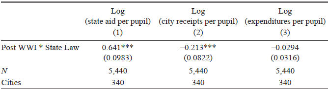
The impact of early grant programs on local school finances has gone largely unexplored in economics. Of particular interest is the question of whether policy changes that increased funds from the state can serve as an instrumental variable for school resources in the spirit of the court-ordered school finance reforms used by Jackson, Johnson, and Persico (2016). We obtained information on which states passed laws mandating major increases in grants from the state to local districts immediately following WWI from the Biennial Survey of Education.Footnote 10 We then ran simple two-way fixed effects regressions on our baseline sample of cities from 1900 to 1930, where we included dummies for the post-WWI period and the passing of a state law increasing grant aid, as well as the interaction of these variables in Table 1. The results suggest that early grant programs crowded out local spending on education.Footnote 11 In states that passed a grant law after WWI, city school districts saw a 90 percent increase in per pupil aid from the state government (Column (1)).Footnote 12 However, the revenues a school received from the city decreased by about 24 percent (Column (2)).Footnote 13 This left expenditures per student unchanged (Column (3)). It thus appears that increased state aid to schools after WWI crowded out local investment in education.Footnote 14 We, therefore, develop a novel instrument for changes in educational resources per pupil using anti-German sentiment.
IMPACTS OF STATE EDUCATIONAL FUNDING LAWS

Table 1 Long description
A table with three columns and four rows, plus a header row. The columns are labeled ‘Log (state aid per pupil)’, ‘Log (city receipts per pupil)’, and ‘Log (expenditures per pupil)’. The row labels are ‘Post WWI * State Law’. The values in the table are as follows: Row 1: Post WWI * State Law, 0.641***, -0.213***, -0.0294. The table also includes additional information such as ‘N’ and ‘Cities’ with values 5,440 and 340 respectively for each column.
Notes: The unit of observation is a city-year. The “Post WWI” variable is an indicator that takes a value of 1 for the years 1917–1930, and a value of 0 for the years 1900–1916. “State Law” is an indicator that takes a value of 1 if a city is located in a state that passed a law increasing state aid to schools after WWI. The states that passed these laws are: Arizona, California, Georgia, Iowa, Louisiana, Massachusetts, New York, North Carolina, Pennsylvania, South Carolina, Texas, Utah, Washington, and West Virginia. State aid per pupil, city receipts per pupil, and expenditures per pupil are interpolated between two adjacent academic years when they are not reported for a city. All regressions control for city and year fixed effects. Standard errors are clustered at the city-level and reported in parentheses.
*** p<0.01.
Source: Schmick and Shertzer (Reference Schmick and Shertzer2025).
DATA
City School Spending Data
We used the Report of the Commissioner of Education (1900–1916) and the Biennial Survey of Education (1918–1930) to construct a new city-level dataset of public school resources during the early twentieth century.Footnote 15 We collected the available data on school resources for every other academic year, beginning with the 1899–1900 academic year.Footnote 16 The reports contain information on expenditures for teachers and supervisors, expenditures for capital, other expenditures, average daily attendance in public schools, the number of public school teachers, and the revenues that city school districts received from city, county, and state governments. These data allow us to compute total expenditures per pupil, which we define as the sum of expenditures for teachers, supervisors, capital, and other expenditures, all divided by the average daily attendance in a city school system. For our analysis, we form a panel of 340 of the largest cities in the United States during the early twentieth century (Schmick and Shertzer Reference Schmick and Shertzer2025).Footnote 17
To provide a more complete picture of the evolution of school resources in the early twentieth century, we graph a time series of real expenditures per pupil and the pupil-teacher ratio by census region in Figure 1. Panel A of Figure 1 shows real expenditures per pupil, which rose only modestly from 1900 to WWI. It is only after 1920 that large real increases are evident. Average real expenditures per pupil increased from $79 in 1920 to $143 in 1924, an 81 percent increase. Panel B graphs the pupil-teacher ratio, which declined steadily from 1900 to about 1920 before leveling off. Figure 1 suggests that increased expenditures after WWI were not simply a matter of smaller class sizes.
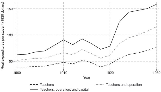
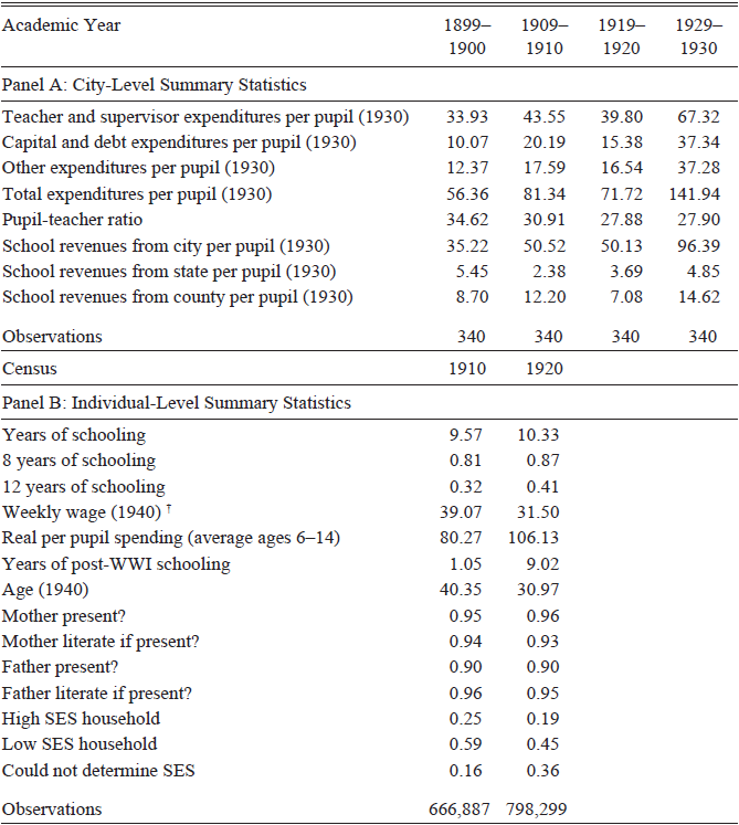
To explore this idea further, Figure 2 breaks the time series of real expenditures per pupil into three main categories of expenditures: expenditures on teachers and supervisors, operations, and capital. The overall trend is that all three expenditure categories increase dramatically after 1920. However, expenditures on capital and operations increase faster than expenditures on teachers and supervisors. Expenditures on teachers and supervisors made up about 60 percent of total expenditures in 1900, but this category dropped to around 50 percent by 1930. Expenditures on capital and operations each made up around 20 percent in 1900, but each of these categories increased to around 25 percent by 1930, reflecting a surge in new school construction and administration. Panel A of Table 2 displays summary statistics for the 340 city school systems in our sample for four academic years: 1899–1900, 1909–1910, 1919–1920, and 1929–1930.
GROWTH IN EDUCATIONAL SPENDING BY CATEGORY
Notes: Data are weighted averages for our sample of 340 cities. The data are weighted by the number of pupils in average daily attendance in each city in every academic year. Real expenditures per student are adjusted using the CPI from Officer and Williamson (Reference Officer and Williamson2021). The year of each data point corresponds to the calendar year in which the academic year ended (e.g., expenditures per pupil for the 1905–1906 academic year are plotted in 1906). The 1914–1915 academic year is plotted in 1916, since we could not find data for the 1915–1916 academic year.
Source: Schmick and Shertzer (Reference Schmick and Shertzer2025).

SUMMARY STATISTICS

Table 2 Long description
The table is divided into two panels: Panel A and Panel B. Panel A presents city-level summary statistics for four academic years: 1899-1900, 1909-1910, 1919-1920, and 1929-1930. It includes data on teacher and supervisor expenditures per pupil, capital and debt expenditures per pupil, other expenditures per pupil, total expenditures per pupil, pupil-teacher ratio, school revenues from city per pupil, school revenues from state per pupil, school revenues from county per pupil, and the number of observations. Panel B presents individual-level summary statistics for the years 1910 and 1920, including years of schooling, 8 years of schooling, 12 years of schooling, weekly wage in 1940, real per pupil spending for average ages 6-14, years of post-WWI schooling, age in 1940, presence of mother and father, literacy of mother and father if present, high and low SES household status, and the number of observations.
Notes: Data in Panel A are from the Report of the Commissioner of Education (1900–1916) and the Biennial Survey of Education (1918–1930). Monetary values in Panel A are in 1930 dollars, which were adjusted using the CPI from Officer and Williamson (Reference Officer and Williamson2021). Data in Panel B are from the linked census sample.
†: There are a different number of observations for weekly wages. The number of observations for each census year is as follows: 402,692 (1910); 523,749 (1920).
Source: Schmick and Shertzer (Reference Schmick and Shertzer2025).
Linked Census Samples
To measure if student outcomes were impacted by the large expansion of school investments associated with WWI, we construct a dataset of White men linked from the 1910 and 1920 complete count censuses to the 1940 complete count census (Ruggles et al. Reference Ruggles, Flood, Goeken, Grover, Meyer, Pacas and Sobek2021). We restrict our attention to White men in light of the concern that Black children did not experience similar exposure to school resources (Baker Reference Baker2019). Linking individuals is necessary to match adults in 1940 to the local level of school resources they experienced as children. We begin by restricting the 1910 and 1920 censuses to White men who were 6 to 15 years of age when the census occurred and were living in one of the 340 cities for which we have school resource data. In other words, the 1910 linked sample includes individuals born 1895–1904, and the 1920 linked sample includes individuals born 1905–1914.
We use the ABE linking algorithm, which was developed by Ran Abramitzky, Leah Boustan, and Katherine Eriksson and used in Abramitzky, Boustan, and Eriksson (Reference Abramitzky, Boustan and Eriksson2012, Reference Abramitzky, Boustan and Eriksson2014), Abramitzky et al. (Reference Abramitzky, Boustan, Jacome and Pérez2021b), and many other papers. We begin by adjusting first names for common nicknames and then standardize each first name and surname using the NYSIIS algorithm, which transforms a word into a phonetic code. We then restrict our sample to individuals who are unique by NYSIIS first name, NYSIIS surname, birthplace, and birth year. For each individual in the 1910 and 1920 censuses, we search for records in the 1940 census that match exactly on NYSIIS first name, NYSIIS surname, birthplace, and birth year. If we find a unique match, then we declare this observation to be a match. If we find multiple matches, then the observation is discarded.
If we do not find a unique match, then we continue to search for individuals who match exactly on NYSIIS first name, NYSIIS surname, and birthplace, but we now allow birth year to differ by up to one year (e.g., if an individual in the 1910 census reports a birth year of 1902, we search for individuals in the 1940 census with a birth year of 1901 and 1903). If no unique match is found, we continue to search for individuals who match exactly on NYSIIS first name, NYSIIS surname, and birthplace, but we now allow birth year to differ by up to two years. The ABE algorithm is one of many algorithms currently used to link individuals across censuses. For other algorithms, see Abramitzky, Mill, and Pérez (Reference Abramitzky, Mill and Pérez2020), Bailey et al. (Reference Bailey, Cole, Henderson and Massey2020), and Feigenbaum (Reference Feigenbaum2016). Importantly, Abramitzky et al. (Reference Abramitzky, Boustan, Eriksson, Feigenbaum and Pérez2021a) show that automated approaches, including the ABE algorithm, result in low false-positive rates and similar coefficient estimates relative to a hand-linked sample.
The results from this linking procedure are displayed in Online Appendix Table A.I. From the 1910 complete count census we searched for 1,995,734 individuals and were able to find 666,887 of them in the 1940 census (a 33 percent link rate); for 1920, we searched for 2,264,425 individuals in 1920 and were able to successfully link 798,299 of them to 1940 (a 35 percent link rate). Our link rates are generally in line with, but a bit higher than, the prior literature. For example, Abramitzky et al. (Reference Abramitzky, Boustan, Jacome and Pérez2021b) were able to successfully link 29.5 percent of individuals from the 1910 census to the 1940 census. This discrepancy in link rates is likely due to the fact that Abramitzky et al. (Reference Abramitzky, Boustan, Jacome and Pérez2021b) link individuals both forward in time (from 1910 to 1940) and backward in time (from 1940 to 1910) and take the intersection of individuals that were linked both ways. We only link forward since we need information on the city an individual was living in as a child, which is not available in the 1940 census. Despite the slightly higher link rates, we show the robustness of our main results to alternative and more conservative matching procedures.
Panel B of Table 2 displays summary statistics for our sample of linked White men. All of the summary statistics are calculated using the number of observations reported at the bottom of the table, except for weekly wages. We construct weekly wages by dividing annual income by the number of weeks worked, both reported for the year 1939. We then follow Acemoglu, Autor, and Lyle (Reference Acemoglu, Autor and Lyle2004) by censoring weekly wages at the 98th percentile and assigning values above the 98th percentile with 1.5 times the 98th percentile wage.Footnote 18 For weekly wages, we include only individuals who were wage workers, worked more than 30 weeks in the year, and were not employed in a work relief program such as the Civilian Conservation Corps or Works Progress Administration.
Online Appendix Table A.I shows that our linked sample appears to be representative of the overall population. For example, the average age of individuals in 1910 that we were able to link was 10.42 years, while the average age of the entire sample that we attempted to link was 10.44 years. We do find that children from families that likely had higher socioeconomic statuses were more likely to be linked. For example, individuals in our linked sample are usually about 3–4 percentage points more likely to live in a dwelling that is owned, as opposed to rented. In addition, the parents of individuals in our linked sample have slightly higher literacy rates, and the fathers have slightly higher occupational income scores (occscores). We address these differences by splitting the sample based on whether the father is of high or low socioeconomic status in some specifications.
Another concern is that individuals in high-German-share cities might be more or less likely to be linked relative to individuals in low-German-share cities. We explore this issue in Online Appendix Table A.II and do not find large discrepancies between the share of individuals linked in high- and low-German-share cities. We were able to successfully link about 33 percent of individuals in low-German-share cities (452,589 out of 1,386,841) and 35 percent of individuals in high-German-share cities (1,012,597 out of 2,873,318). Additionally, we find that the linked samples in both types of cities appear representative of the overall population, with the caveat that children from families that likely had higher socioeconomic statuses were more likely to be linked (as is the case for most census linking papers). We believe that, if anything, this might bias us toward not finding an impact of educational expenditures on adult outcomes for two reasons. First, children from high socioeconomic status families were more likely to be enrolled in private schools, which means that our school expenditure measure, which is only relevant for public schools, is not accurate for them. Second, even if children from high socioeconomic status families did attend public school (which many did), they had a variety of channels not available to low socioeconomic status children that might break any potential relationship between school expenditures and adult outcomes (such as private tutors, family business networks, etc.).
EMPIRICAL STRATEGY
Panel Estimation Using OLS
The objective of our empirical work is to identify the causal effect of the large increases in school resources that occurred during the early twentieth century on adult outcomes. We begin with a naïve estimation of the effect in a panel framework using the following specification:

In Equation (1), i indexes individuals, e indexes city-of-education, and c indexes cohorts. [outcome]iec is one of four adult outcomes: (1) years of schooling, (2) the probability of completing eight years of schooling, (3) the probability of completing 12 years of schooling, and (4) weekly wages. We restrict the sample to men born between 1895 and 1913 because our school resource data covers the 1900 to 1930 period, and we can thus only compute an average of expenditures per pupil for all 13 school-age years (in other words, 5–17 years of age) for these cohorts.Footnote 19 When weekly wages are the dependent variable, we restrict the sample to wage workers who worked more than 30 weeks in the year and who were not employed in a work relief program. Importantly, self-employed individuals (including farmers) did not report income in the 1940 census and, therefore, we could not compute weekly wages for them; they are not included in the sample when weekly wages are the dependent variable. Since our sample consists primarily of individuals in urban areas and does not include many farmers, only 13 percent of our sample is self-employed.Footnote 20
The vector X iec contains individual-level characteristics including: mother’s literacy (three dummy variables: mother literate, mother illiterate, and mother not present), father’s literacy (three dummy variables: father literate, father illiterate, and father not present), mother’s occupation (dummies), father’s occupation (dummies), father’s birthplace (dummies), mother’s birthplace (dummies), own birthplace (dummies), and childhood home ownership status (dummies for owned, rented, or unknown).Footnote 21 The vector Y ec contains city-of-education by cohort-level controls, including the average percentage of each city’s population employed in various professions during each cohort’s mandatory school-age years. In particular, we control for the percentage of a city’s population employed as a professional, craftsman, operator, service worker, laborer, or farmer (non-occupational responses are the omitted category).Footnote 22 Y ec also controls for the average number of mandatory school years, which are defined for each birth cohort based on state compulsory schooling laws. We subtract the work permit age from the entry age for states that had work permit laws. For states without work permit laws, we subtract the exit age from the entry age. Data on entry, exit, and work permit ages are taken from Goldin and Katz (Reference Goldin and Katz2008).
We include cohort fixed effects γ c and city-of-education fixed effects γ e. For our main treatment variable, we construct a measure of a student’s exposure to school resources, [ln expenditures per pupil]ec, which is the log of average expenditures per pupil (in real 1930 dollars) during potential school-age years (ages 5–17 during our time period) for individuals in cohort c who were educated in city e. Finally, τ iec is a stochastic error term, and we cluster standard errors at the city-of-education level.
For Equation (1) to estimate a causal effect, it must be the case that, conditional on the controls in Y ec, per pupil expenditures were randomly assigned to city school districts. This assumption, undoubtedly, does not hold. Thus, our primary concern in Equation (1) is that the OLS panel estimates are biased. For example, cities with booming labor markets could increase school expenditures (perhaps from increases in the tax base), and student outcomes could improve through mechanisms unrelated to school expenditures, biasing our results away from zero. Alternatively, if cities made dynamic investment decisions and increased spending by more when schooling outcomes were deteriorating, estimated impacts of school resources would likely be biased toward zero. The narrative history certainly suggests that reformers lobbied for larger school budgets in response to the poor performance of “foreign elements” in the school system during the period of generally high immigration before 1924. To address the endogeneity of expenditures per pupil, we next discuss our instrumental variables approach, which aims to isolate variation in school resources that is uncorrelated with trends in student outcomes.
Instrumental Variables Approach Using Anti-German Sentiment
Our instrumental variables approach exploits variation in educational spending that arose as a result of anti-German sentiment as opposed to concerns about schooling outcomes. Specifically, we construct a measure of exposure to years of education after WWI, interacted with the share of the population in a city that was of German descent in 1910, prior to WWI. Our approach shares some similarities with Acemoglu, Autor, and Lyle (Reference Acemoglu, Autor and Lyle2004), who use county German share to obtain variation in WWII mobilization rates uncorrelated with economic conditions. In this section, we show that our instrument is predictive of future increases in educational spending and that German share, not general immigrant levels, is driving increases in investments. Finally, we provide a set of checks on the exclusion restriction, including showing that cities with different German shares were not on different trajectories of wages or years of schooling prior to WWI.
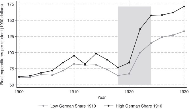
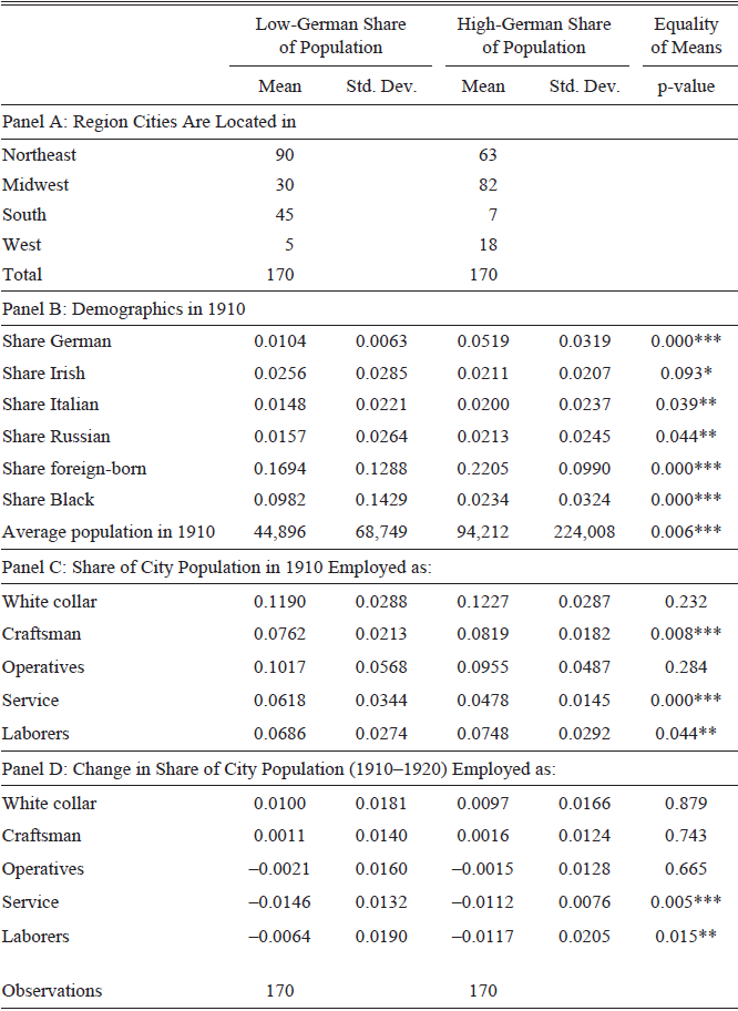
We visualize the basic variation underlying our instrument in Figure 3. Here, we subdivide our sample of cities by median German population share and show trends in spending per pupil.Footnote 23 Prior to WWI, cities with higher German shares of the population spent more on education than cities with lower German shares. The level differences arise largely as a function of geography, with German immigrants having settled predominantly in the large, industrial cities of the Midwest and Northeast and having largely avoided the South (see Panel A of Table 3). Importantly, cities with high-German shares do not appear to have been on a different trend in expenditures per pupil for at least ten years prior to WWI. In 1908, cities with high-German shares had expenditures per pupil that were 17 percent higher than cities with low-German shares ($84.37 vs. $72.06). Ten years later, in 1918, the difference was 19 percent ($76.80 vs. $64.50). However, after 1918, the gap between expenditures per pupil in high- and low-German-share cities began to widen. By 1924, the gap had reached 37 percent, almost double the level in 1918.Footnote 24 All cities increased expenditures in the aftermath of WWI (as is obvious from Figure 3), but cities with large German populations differentially increased their expenditures.
GROWTH IN EXPENDITURES PER PUPIL BY GERMAN SHARE
Notes: Data are weighted averages for cities in each group. The data are weighted by the number of pupils in average daily attendance in each city in every academic year. High and low German share are defined as cities above and below the median German share of the population, which is 2.26 percent of the population.
Source: Schmick and Shertzer (Reference Schmick and Shertzer2025).

DIFFERENCE IN CHARACTERISTICS OF CITIES BY GERMAN SHARE

Table 3 Long description
The table is divided into four panels (A, B, C, D) and compares various characteristics of cities with low and high German shares of the population. Panel A shows the regions where cities are located, with means and standard deviations for both low and high German shares. Panel B provides demographic data from 1910, including shares of different ethnic groups and the average population. Panel C details the share of the city population employed in different occupations in 1910. Panel D shows the change in the share of the city population employed in various occupations from 1910 to 1920. Each panel includes p-values to indicate the equality of means between the two groups.
Notes: This table shows average characteristics in 1910 for the 340 cities in our sample. There are 170 cities in the “Low-German share of population” group and 170 cities in the “High-German share of population” group. White collar workers are defined as professionals, managers, officials, proprietors, clerks, and salesmen. The final column provides the p-value from a test for the equality of means (t-test) between low- and high-German-share cities.
* p<0.1, ** p<0.05, *** p<0.01.
Source: Schmick and Shertzer (Reference Schmick and Shertzer2025).
Having introduced our instrument, we can estimate the following system of equations using two-stage least squares (2SLS):


In Equations (2) and (3), γ c and θ c are cohort fixed effects, γ e and θ e are city-of-education fixed effects, X iec are individual level control variables, and Y ec are city-of-education by cohort level controls. These controls are the same as those from Equation (1). [exposure]c is the number of years of schooling for cohort c that occurred after the United States entered WWI in 1917. We again define school-age years as being 5 to 17 years old. Therefore, [exposure]c is zero for individuals born in or before 1900, one for individuals born in 1901, and two for individuals born in 1902, and takes a maximum value of 13 for individuals born in 1913 (the last birth cohort in our sample). Finally, [German share 1910]e is the German share of the population in 1910 for city-of-education e.
In order for the German share of the population in 1910 interacted with exposure to years of education after WWI to be a suitable instrument for educational expenditures, it must satisfy two criteria. First, it must be the case that the presence of Germans specifically prompted increased spending on education around the time of the war, when fears of enemy aliens peaked. Second, it must satisfy the exclusion restriction, which states that the German share of the population in 1910 impacted student outcomes only through its effect on expenditures per pupil.
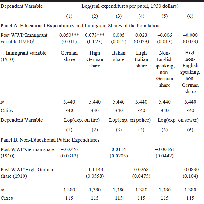
We explore the first criterion in Panel A of Table 4. All columns in this table control for city and year fixed effects and the share of a city’s population working in the following occupations: white collar (professional, manager, clerk, or salesman), craftsman, operator, service worker, laborer, or farmer. Column (1) of Table 4 uses the German share of a city’s population in 1910, which has been standardized to have a mean of zero and a standard deviation of one. A one standard deviation increase in the German share of a city’s population resulted in a 5 percent increase in expenditures per pupil after WWI. Column (2) dichotomizes the German share measure and shows that cities with above median German shares of the population in 1910 increased expenditures per pupil after WWI by 7 percent relative to cities with low-German shares.Footnote 25 We show in Columns (3) and (4) of Table 4 that this was a phenomenon specific to Germans, as we do not find a similar effect for Italian immigrants. Finally, Columns (5) and (6) show that having a high-German population, not a high foreign-born population more generally, is what led to the divergence in expenditures per pupil using both dichotomous and continuous measures of non-English-speaking, non-German immigrants.
VALIDITY OF GERMAN SHARE INSTRUMENT

Table 4 Long description
The table is divided into two panels: Panel A and Panel B. Panel A focuses on educational expenditures and immigrant shares of the population, while Panel B focuses on non-educational public expenditures. Panel A has six columns and five rows, including the header row. The columns are labeled with different immigrant share variables and their impact on log(real expenditures per pupil, 1930 dollars). The rows include the Post WWI*Immigrant variable (1910) and its interaction with different immigrant shares, along with the number of observations (N) and cities. Panel B has three columns and four rows, including the header row. The columns are labeled with different expenditure variables and their impact on log(exp. on fire), log(exp. on police), and log(exp. on sewer). The rows include the Post WWI*German share (1910) and Post WWI*High-German share (1910), along with the number of observations (N) and cities. The table provides specific values for each interaction, indicating the impact of immigrant shares on expenditures.
Notes: The unit of observation is a city-year. The “Post WWI” variable is an indicator that takes a value of one for the years 1917–1930, and zero for the years 1900–1916. “German share (1910)” is the share of a city’s population that were immigrants from Germany in 1910. “Italian share (1910)” is the share of a city’s population that were immigrants from Italy in 1910. “Non-English speaking, non-German share (1910)” is the share of a city’s population that were immigrants and not from Canada, England, Germany, Ireland, Northern Ireland, Scotland, and Wales. All continuous measures are standardized to have a mean of zero and standard deviation of one. “High-German share (1910)” is an indicator if a city had an above median German share of the population in 1910. “High Italian share (1910)” is an indicator if a city had an above median Italian share of the population in 1910. “High non-English speaking, non-German share (1910)” is an indicator if a city had an above median non-English speaking, non-German share of the population in 1910. All regressions control for city fixed effects, year fixed effects, and the share of a city’s population working in the following occupations: white collar (professional, manager, clerk, or salesman), craftsman, operator, service worker, laborer, or farmer. Spending on fire, police, and sewer services were provided by Elyce Rotella and Louis Cain. Standard errors are clustered at the city-level and are reported in parentheses.
*** p<0.01.
Source: Schmick and Shertzer (Reference Schmick and Shertzer2025).
We now turn to the exclusion restriction. One concern regarding the validity of our instrument is whether cities with high-German shares of the population were on systematically different trajectories from cities with lower German shares of the population. For example, if German immigrants had a preference for settling in cities with growing tax bases and increasing expenditures on public schools, then this tendency would invalidate our argument that city schools responded to the German share of the population by increasing expenditures after WWI. We provide evidence that German immigrants were not simply clustered in cities with better tax bases in Panel B of Table 4. Specifically, we run a series of regressions on 115 cities for which we obtained non-educational public expenditure data on fire, police, and sewer services.Footnote 26 These regressions, shown in Panel B of Table 4, demonstrate that the German share of a city’s population does not appear to have significantly impacted non-educational public expenditures after WWI. If anything, such cities spent less on these other public goods. These results strongly suggest that German share is not simply a proxy for a growing post-WWI tax base.
A related concern (and violation of the exclusion restriction) is that cities or regions with more Germans were on different trends along some dimensions that would somehow have led to differing evolutions of educational attainment or wages in the absence of increased educational spending. For instance, it could be the case that areas with more Germans were shifting out of manufacturing and into white-collar work more rapidly. To explore this idea, Panels B through D of Table 3 examine demographic and economic characteristics of cities based on the German share of the population. Panel B shows that cities with high-German shares had larger populations and a smaller Black share, which is consistent with few Germans settling in the South (Panel A). Panel C shows that while there are some significant differences in the industrial composition of high- and low-German-share cities, these differences are generally small in magnitude (less than 2 percentage points). Perhaps more important than the level differences shown in Panel C is the question of whether high-German-share cities were trending differently. Accordingly, Panel D shows changes in occupational shares of the city between 1910 and 1920. There were some small differences in the decline of low-skill occupations in high- versus low-German-share cities between 1910 and 1920. We, therefore, include controls for occupational structure in our baseline specifications. We also show our main results are robust to the inclusion of region time-trends and to dropping the “German Triangle” (the high-German area between St. Louis, Milwaukee, and Cincinnati).
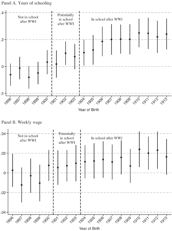
Our instrument is, essentially, a difference-in-differences setup and, therefore, is subject to the usual difference-in-differences parallel trends assumption. A recent literature has also highlighted the importance of the assumptions made about the trends in outcomes absent treatment (for instance, see De Chaisemartin and D’HaultfOEuille 2017; Goodman-Bacon Reference Goodman-Bacon2018). In our context, we must assume that the difference in outcomes between children educated in high- versus low-German-share cities would have trended similarly had WWI not occurred. We estimate the following event study specification to provide some evidence on this:

This equation is similar to Equation (1), but we replace expenditures per pupil with a series of birth cohort dummy variables (γ c; omitting 1894) interacted with a dummy variable if the individual was educated in a high-German-share city. We wish to demonstrate that individuals living in high-German-share cities and who were completely educated prior to WWI had similar outcomes to those living in low-German-share cities.
We plot the coefficients φ c in Figure 4. Panel A shows the coefficients when years of schooling is the dependent variable. There is no significant difference in years of schooling for individuals living in high-German-share cities who were completely educated prior to WWI (the 1895–1900 birth cohorts). We begin to see an upward trend in years of schooling for individuals educated in high-German-share cities starting with the 1901 birth cohort. The 1901–1903 birth cohorts could have been in high school during and shortly after WWI, so individuals from high-German-share cities would have experienced some of the rapid, war-induced increase in expenditures. Finally, because compulsory schooling laws mandated most children to stay in school until at least the age of 14, the 1904 birth cohort and all later cohorts were definitely exposed to some post-WWI education. Accordingly, the upward trend that started in 1901 is more pronounced for these cohorts. Panel B of Figure 4 plots the coefficient estimates when log of weekly wage is the dependent variable. Again, we see no upward trend prior to the 1901 birth cohort.
ESTIMATED DIFFERENCES IN OUTCOMES BY CITY GERMAN SHARE
Notes: The unit of observation is an individual. The figure graphs the coefficient estimates from Equation (4) in the text. The points are the difference in outcomes between high- and low-German-share cities relative to 1895 (the omitted year). Ninety-five percent confidence intervals are shown.
Source:Schmick and Shertzer (Reference Schmick and Shertzer2025).

We also illustrate the trend in school spending by German share in Online Appendix Figure A.III. Estimated differences in average expenditures per student are essentially flat for cohorts born between 1898 and 1904, after which high-German-share cities begin to spend more. Taken together, all these pieces of evidence are consistent with the exclusion restriction holding.
RESULTS
Main Results
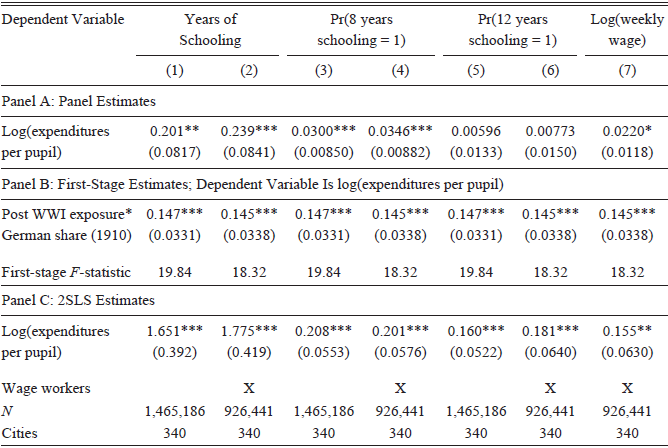
We begin our analysis by estimating Equations (1)–(3) for our four outcomes of interest. Panel A of Table 5 presents the baseline panel regression estimates. Columns (1), (3), and (5) use the entire sample of individuals for whom we have years of schooling, while Columns (2), (4), (6), and (7) use the sample of individuals who were wage workers. Consistent with the expectation that the naïve OLS estimation would be biased downward, nearly all of the panel estimates are small, even when they are significantly different from zero. For example, in Column (1) of Panel A, a 10 percent increase in expenditures per pupil during school-age years would result in a 0.0201-year increase in years of schooling, or about 3.5 additional days of school for a typical 180-day school year.
OLS AND 2SLS ESTIMATES OF EXPENDITURES PER PUPIL ON ADULT OUTCOMES

Table 5 Long description
A table with three panels (A, B, and C) showing estimates of expenditures per pupil on adult outcomes. Panel A presents baseline panel regression estimates with columns for years of schooling and probabilities of 8 and 12 years of schooling, and log of weekly wage. Panel B shows first-stage estimates with log of expenditures per pupil as the dependent variable. Panel C displays 2SLS estimates with the same outcomes as Panel A. Each panel includes statistical values and significance levels. Panel A has seven columns with different dependent variables and samples. Panel B has one row with post-World War II exposure and German share. Panel C has seven columns similar to Panel A but with 2SLS estimates.
Notes: The unit of observation is an individual. Panel A provides estimates of Equation (1), Panel B provides estimates of Equation (2), and Panel C provides estimates of Equation (3). The treatment variable, log(expenditures per pupil), is average per pupil spending (in real 1930 dollars) during the years an individual was aged 5–17. Expenditures per pupil is the sum of expenditures on teachers, supervisors, capital, and other expenditures all divided by the average daily attendance in a city-year cell. All regressions control for: city-of-education fixed effects, birth year fixed effects, mother’s literacy (dummy variables for mother literate, mother illiterate, and mother not present), father’s literacy (dummy variables for father literate, father illiterate, and father not present), mother’s occupation (dummies), father’s occupation (dummies), mother’s birthplace (dummies), father’s birthplace (dummies), own birthplace (dummies), childhood home ownership status (dummies for owned, rented, or unknown), the average number of mandatory school years, and the average percent of a city’s population that works in various occupations. The average number of mandatory school years, which we control for, is defined for each birth cohort based on state compulsory schooling laws. In particular, we subtract the work permit age from the entry age for states that had work permit laws. For states without work permit laws, we subtract the exit age from the entry age. Data on entry, exit, and work permit age are taken from Goldin and Katz (Reference Goldin and Katz2008). We control for the average percent of a city’s population working in the following occupations: white collar (professional, manager, clerk, or salesman), craftsman, operator, service worker, laborer, or farmer. Non-occupational responses are the omitted category. These percentages were constructed from the 1900–1930 IPUMS (Ruggles et al. Reference Ruggles, Flood, Goeken, Grover, Meyer, Pacas and Sobek2021) complete count census data and are interpolated between census years. Standard errors are clustered at the city-level and reported in parentheses.
* p<0.1, ** p<0.05, *** p<0.01.
Source: Schmick and Shertzer (Reference Schmick and Shertzer2025).
Panel B of Table 5 reports on the first stage from our 2SLS regressions. The F-statistic in the first stage is around 20 in all cases, indicating a sufficiently strong first stage. Panel C reports the coefficients from the second stage of our 2SLS approach. Column (1) shows that a 10 percent increase in expenditures per pupil during mandatory school-age years increased years of schooling by 0.17 school years. For a typical 180-day school year, this effect translates into approximately 30 additional days of schooling. In Columns (3)–(6) we find that a 10 percent increase in expenditures per pupil increased the probability of completing 8 and 12 years of schooling by about 2 percentage points. Finally, Column (7) shows that a 10 percent increase in expenditures per pupil led to a 1.6 percent increase in adult wages.Footnote 27
To put these results into context, the average student in our sample saw expenditures per pupil increase by 0.34 log points (or 40 percent) over his 13 school-age years (5 through 17), and years of schooling in our sample increased by 1.3 from the 1895 cohort to the 1913 cohort.Footnote 28 If our 2SLS point estimate (1.65) of the relationship between log educational expenditures and years of schooling is taken seriously, this implies that increased educational expenditures should increase years of schooling by 0.56 years (1.65*0.34), which accounts for 43 percent (0.56/1.3) of the increase in years of schooling over our sample period. The same average increase in expenditures translated into wage increases of 6 percent.Footnote 29
It is useful to compare our main results to modern estimates of the impact of school resources on long-run outcomes. One such set of estimates comes from Jackson, Johnson, and Persico (2016). They look at children born between 1955 and 1980 and find that a 10 percent increase in expenditures per pupil resulted in 0.31 more years of completed schooling and 7 percent higher wages. Recall that for a similar 10 percent increase, we find that years of schooling would increase by 0.17 years and weekly wages by about 1.6 percent. Thus, our results are generally smaller in magnitude than those of Jackson, Johnson, and Persico (2016). There could be several reasons for these differences. First, it is possible that the returns on school resources have changed over time. Perhaps schooling is more valuable in the modern era due to changes in the occupational and industrial structure of the United States. A second potential source of difference between estimates is that Jackson, Johnson, and Persico (2016) instrument for expenditures per pupil with court-ordered school finance reforms, whereas we use the share of the German population in a city prior to WWI.
Robustness
We next explore the robustness of these results to the inclusion of regional time trends to address the concern that areas with more Germans were evolving differently along unobservable dimensions in terms of wages or educational attainment. Online Appendix Table A.V reports the results of the baseline specification with the addition of four census region time trends, which, for instance, allow the “German Triangle” in the Midwest to have a different trend relative to the Northeast. Our estimates for attainment, completing eight years of schooling, and wages are similar, but the estimated effect on 12 years of schooling drops by about half and loses significance. We also reran the baseline specification on the sample of cities outside the “German Triangle” in Online Appendix Table A.VI and found results similar to the baseline specification.Footnote 30 We conclude that the German share instrument may be picking up some regional trends in high school completion. However, it appears unlikely that trends in attainment at lower rungs of the educational ladder or in wages are being driven by general trends across regions that are correlated with German share.
We explore whether large or small cities are driving our results in Online Appendix Table A.VII by dropping individuals educated in cities whose populations were over 250,000 in 1900. The 2SLS estimates are displayed in Panel B, and our first stage is even stronger for this subsample, with F-statistics over 25. The coefficient estimates remain similar to Table 5, with the exception of the coefficient estimate for weekly wages, which is smaller. Only 17 cities in our sample have populations over 250,000, indicating that our effects are not simply being driven by the large cities. In fact, it could be the case that our instrument has more power in this subsample if German immigrant populations are more noticeable in smaller cities.
Individuals born after 1910 would be under the age of 30 in 1940 and may not have achieved their full earning potential. We explore the robustness of our results to an age restriction in Online Appendix Table A.VIII by dropping individuals born after 1910. We find that our results are generally robust to this restriction and our first stage remains sufficiently strong.
Alternative Linking Methods
Our main results use the ABE linking algorithm. However, Bailey et al. (Reference Bailey, Cole, Henderson and Massey2020) show that automated linking algorithms that use phonetically cleaned names can result in a large number of false-positive matches (in other words, linking a child to the wrong adult). The rate of false positives in our sample would have to be systematically related to both the German share of a city’s population and the years in which a child was educated for our results to be confounded by false positives (e.g., many false positives for children educated in all places prior to WWI, but few false positives for children educated in high-German-share cities after WWI). While we believe this is unlikely, we nevertheless follow Abramitzky et al. (Reference Abramitzky, Boustan, Jacome and Pérez2021b) and use three more conservative linking techniques to demonstrate the robustness of our results.
First, we restrict our sample to individuals that match exactly on first name (not phonetically cleaned), last name (not phonetically cleaned), birthplace, and birth year. We re-estimate our main empirical results (Table 5) with this sample and display the results in Online Appendix Table A.IX. The results using only individuals that match exactly on name and birth year are almost identical to our main results. The second method restricts to individuals whose NYSIIS cleaned first and last names are unique within a five-year age band. We again re-estimate Table 5 using the unique names and display the results in Online Appendix Table A.X. The results are again almost identical to our main results. Finally, we restrict to individuals that match exactly on name and birth year and that are unique within a five-year age band. The results using this method remain similar and are displayed in Online Appendix Table A.XI. It therefore appears unlikely that our results are sensitive to the inclusion of false positives, since more conservative linking approaches—which should result in fewer false-positive matches—yield similar results.
Heterogeneous Effects by Socioeconomic Status and Nativity
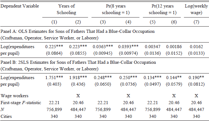
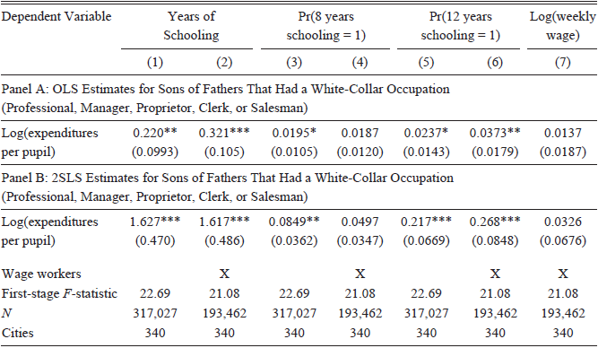
The early twentieth century was a time of significant inequality. An advantage of our approach is that we can assess the returns to school resources for children from different economic backgrounds. Table 6 shows our results for children whose fathers had a blue-collar job, which we define as being a craftsman, operative, service worker, or laborer. Table 7 shows the corresponding results for children whose fathers had a white-collar job, which included professionals, managers, proprietors, clerks, or salesmen.
EFFECT OF SCHOOL RESOURCES ON ADULT OUTCOMES FOR SONS OF LOW SES FATHERS

Table 6 Long description
The table is divided into two panels: Panel A and Panel B. Panel A presents OLS estimates for sons of fathers that had a blue-collar occupation, while Panel B presents 2SLS estimates for the same group. The table has seven columns: Dependent Variable, Years of Schooling, Pr(8 years schooling = 1), Pr(12 years schooling = 1), and Log(weekly wage). Each panel contains rows with data on log(expenditures per pupil) and wage workers. The table includes statistical values such as coefficients and standard errors, along with first-stage F-statistics, sample sizes (N), and the number of cities. Panel A shows data for log(expenditures per pupil) and its impact on years of schooling and probabilities of completing 8 and 12 years of schooling, as well as log(weekly wage). Panel B provides 2SLS estimates for the same variables. Notable trends include the positive coefficients for log(expenditures per pupil) in both panels, indicating a positive relationship with years of schooling and probabilities of completing 8 and 12 years of schooling.
Notes: The unit of observation is an individual. The treatment variable, log(expenditures per pupil), is average per pupil spending (in real 1930 dollars) during the years an individual was aged 5–17. Expenditures per pupil is the sum of expenditures on teachers, supervisors, capital, and other expenditures all divided by the average daily attendance in a city-year cell. All regressions control for: city-of-education fixed effects, birth year fixed effects, mother’s literacy (dummy variables for mother literate, mother illiterate, and mother not present), father’s literacy (dummy variables for father literate, father illiterate, and father not present), mother’s occupation (dummies), father’s occupation (dummies), mother’s birthplace (dummies), father’s birthplace (dummies), own birthplace (dummies), childhood home ownership status (dummies for owned, rented, or unknown), the average number of mandatory school years, and the average percentage of a city’s population that works in various occupations. See notes to Table 5 for more details on these controls. Standard errors are clustered at the city-level and reported in parentheses.
** p<0.05, *** p<0.01.
Source: Schmick and Shertzer (Reference Schmick and Shertzer2025).
EFFECT OF SCHOOL RESOURCES ON ADULT OUTCOMES FOR SONS OF HIGH SES FATHERS

Table 7 Long description
A table comparing the effect of school resources on adult outcomes for sons of high SES fathers. The table has 7 columns and 10 rows, including headers and grouped rows. Column headers are Dependent Variable, Years of Schooling, Pr(8 years schooling = 1), Pr(12 years schooling = 1), Log(weekly wage). Row labels include Panel A: OLS Estimates for Sons of Fathers That Had a White-Collar Occupation and Panel B: 2SLS Estimates for Sons of Fathers That Had a White-Collar Occupation. Each panel contains rows with values for Log(expenditures per pupil), Wage workers, First-stage F-statistic, N, and Cities. Panel A has 5 rows and Panel B has 6 rows. Values are provided for each dependent variable and statistical measure.
Notes: The unit of observation is an individual. The treatment variable, log(expenditures per pupil), is average per pupil spending (in real 1930 dollars) during the years an individual was aged 5–17. Expenditures per pupil is the sum of expenditures on teachers, supervisors, capital, and other expenditures all divided by the average daily attendance in a city-year cell. All regressions control for: city-of-education fixed effects, birth year fixed effects, mother’s literacy (dummy variables for mother literate, mother illiterate, and mother not present), father’s literacy (dummy variables for father literate, father illiterate, and father not present), mother’s occupation (dummies), father’s occupation (dummies), mother’s birthplace (dummies), father’s birthplace (dummies), own birthplace (dummies), childhood home ownership status (dummies for owned, rented, or unknown), the average number of mandatory school years, and the average percentage of a city’s population that works in various occupations. The 1911–1913 birth cohorts are not included in the analysis. See notes to Table 5 for more details on these controls. Standard errors are clustered at the city-level and reported in parentheses.
* p<0.1, ** p<0.05, *** p<0.01.
Source: Schmick and Shertzer (Reference Schmick and Shertzer2025).
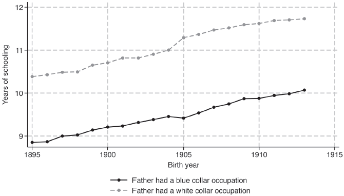
We find that expenditures per pupil had large, positive, and significant effects on all outcomes for the children of low socioeconomic status, blue-collar fathers. Specifically, we find that a 10 percent increase in expenditures per pupil would have increased educational attainment by about 0.2 school years (approximately 36 days), the probability of completing eight years of schooling by 2.5 percentage points, and weekly wages by 2 percent. In comparison, we find that expenditures per pupil had much smaller effects on weekly wages and completing eight years of schooling for the children of high socioeconomic status, white-collar fathers. Children of both low and high socioeconomic status fathers saw increases in the probability of completing 12 years of schooling, but we caution against interpreting this effect as causal in light of our findings related to regional trends. Despite the results generally being larger among the children of low socioeconomic status fathers, we do not find evidence that the gap in years of schooling between low and high socioeconomic students closed for the cohorts in our sample. Figure 5 shows that the gap in years of schooling remained relatively constant at over one year for all cohorts in our sample, suggesting that the increase in school resources helped children from less privileged backgrounds keep up with peers from wealthier families.
GAP IN YEARS OF SCHOOLING IN 1940 BY FATHER’S SOCIOECONOMIC STATUS
Notes: The plotted data are the average years of schooling of individuals in our sample whose father had a blue- or white-collar occupation when we observed the child (in 1910 or 1920). Blue collar occupations are defined as: craftsmen, operators, service workers, or laborers. White collar occupations are defined as: professionals, managers, proprietors, clerks, or salesmen.
Source: Schmick and Shertzer (Reference Schmick and Shertzer2025).

Why are the effects of increased school resources concentrated among the children of lower-skilled workers? One explanation is that the children of professionals were frequently enrolled in private schools and academies in the early twentieth century and, with high parental incomes, would have completed eighth grade regardless of the quality of public schooling in their city. We cannot test for the role of private schools directly; nonetheless, we believe that improved public school quality would have had a larger scope to impact children who could not afford private education. The difference in estimated effects across children of different socioeconomic statuses also suggests that Progressive Era reformers followed through on their intentions to use increases in public funds to improve educational outcomes for working-class youth.
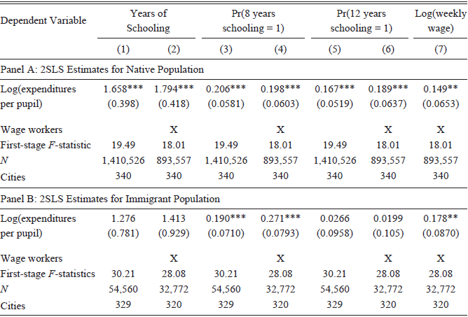
Many of the lower-status workers and their children were foreign-born. We, therefore, also consider differential impacts by nativity. This question is of particular interest since our instrument uses variation in school resources related to anti-German sentiment. We subdivide our sample by nativity and rerun our analysis in Table 8. Panel A shows the 2SLS results for the native-born population, while Panel B shows the results for the foreign-born population. We find that the effects of increased expenditures on high school completion were larger for native-born individuals, while the effects on adult wages were similar across the two groups. Immigration significantly declined during WWI, and after the Emergency Quota Act was passed in 1921, only a relatively small share of our sample (about 3 percent) were foreign-born and of school age in the 1920s. Thus, although increases in school resources resulted from concerns about immigrant assimilation, the native-born (including second-generation immigrants) saw broad benefits.
EFFECT OF SCHOOL RESOURCES ON ADULT OUTCOMES BY NATIVITY

Table 8 Long description
A table comparing the effect of school resources on adult outcomes for native and immigrant populations. The table has two panels: Panel A for native population and Panel B for immigrant population. Each panel includes columns for years of schooling, probability of 8 years of schooling, probability of 12 years of schooling, and log of weekly wage. Panel A shows 2SLS estimates for the native population with rows for log of expenditures per pupil, wage workers, first-stage F-statistic, sample size (N), and number of cities. Panel B shows similar data for the immigrant population. Each row provides specific values and standard errors in parentheses. Notable trends include higher effects of increased expenditures on high school completion for native-born individuals and similar effects on adult wages across both groups.
Notes: The unit of observation is an individual. The treatment variable, log(expenditures per pupil), is average per pupil spending (in real 1930 dollars) during the years an individual was aged 5–17. Expenditures per pupil is the sum of expenditures on teachers, supervisors, capital, and other expenditures all divided by the average daily attendance in a city-year cell. All regressions control for: city-of-education fixed effects, birth year fixed effects, mother’s literacy (dummy variables for mother literate, mother illiterate, and mother not present), father’s literacy (dummy variables for father literate, father illiterate, and father not present), mother’s occupation (dummies), father’s occupation (dummies), mother’s birthplace (dummies), father’s birthplace (dummies), own birthplace (dummies), childhood home ownership status (dummies for owned, rented, or unknown), the average number of mandatory school years, and the average percentage of a city’s population that works in various occupations. See notes to Table 5 for more details on these controls. Standard errors are clustered at the city-level and reported in parentheses.
** p<0.05, *** p<0.01.
Source: Schmick and Shertzer (Reference Schmick and Shertzer2025).
Mechanisms
We conclude our empirical analysis by considering mechanisms through which expenditures per pupil improved student outcomes. To do this, we decompose expenditures into three components: expenditures per pupil on teachers and supervisors, expenditures per pupil on operation expenditures (catch-all category that includes expenditures on clerical work, fuel, heating, textbooks, water, etc.), and expenditures per pupil on capital projects. This decomposition allows us to examine how schools were spending money and, therefore, which elements of expenditures led to improved outcomes.
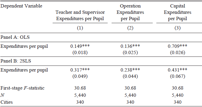
Panel A of Table 9 regresses each of these three components on total expenditures per pupil, city fixed effects, and year fixed effects. Each column in this table can be interpreted as the amount each category of spending would increase by from a one-dollar increase in per pupil spending (in other words, the coefficients across categories of expenditures should add up to 1). Accordingly, for a one-dollar increase in expenditures per pupil, about 15 cents went to teachers, 11 cents went to operations, and 74 cents went to capital projects.
DECOMPOSITION OF EXPENDITURES PER PUPIL

Table 9 Long description
The table presents data on expenditures per pupil across three categories: Teacher and Supervisor Expenditures per Pupil, Operation Expenditures per Pupil, and Capital Expenditures per Pupil. It is divided into two panels: Panel A (OLS) and Panel B (2SLS). Each panel shows the expenditures per pupil with corresponding standard errors in parentheses. Panel A includes the following rows: Expenditures per pupil with values 0.149, 0.136, and 0.709 for the three categories respectively. Panel B includes the following rows: Expenditures per pupil with values 0.317, 0.238, and 0.431 for the three categories respectively. Additionally, Panel B includes a First-stage F-statistic of 30.68, a sample size (N) of 5,440, and 340 cities.
Notes: The unit of observation is a city-year. Expenditures per pupil are total expenditures per pupil. We decompose this aggregate measure into three constituent parts: teacher and supervisor expenditures per pupil, operation expenditures per pupil (catch-all category that includes expenditures on clerical work, fuel, heating, textbooks, water, etc.), and capital expenditures per pupil. All regressions control for city fixed effects and year fixed effects. Standard errors are clustered at the city-level and reported in parentheses.
*** p<0.01.
Source: Schmick and Shertzer (Reference Schmick and Shertzer2025).
The implication of most money going toward capital projects is that city school districts were likely constructing new middle and high schools, which might have encouraged students to stay in school beyond sixth grade. However, when we instrument for expenditures per pupil using the German share interacted with a post-WWI indicator in Panel B, the coefficient on capital expenditures is reduced somewhat, although still the largest of the three categories. One interpretation of these results is that while all cities dedicated increased spending to new schools, cities with high-German shares of the population dedicated relatively more money toward instruction, perhaps on matters of civics and English, and relatively less money toward new schools.
CONCLUSION
This paper documents that WWI was a pivotal moment in the history of educational spending in the United States. In the decade following the conflict, the level of financial support received by urban school districts permanently shifted upward. We provide the first quantitative analysis of the returns on these resources, highlighting several key facts about this historical event. First, overall increases in per pupil spending were generated by cities themselves, not transfers from state governments. Second, while all cities increased spending, urban areas with a larger share of enemy aliens saw proportionally larger growth in school resources. We argue this divergence was related to the assimilation prerogative of cities after the outbreak of WWI and use German share as an instrument for changes in school resources.
As in the present day, using endogenous increases in educational spending leads to estimated returns on school resources that are close to zero. However, using variation arising from the distribution of the German population prior to WWI leads to estimated returns that are statistically significant and economically meaningful. Our results suggest that war-driven increases in spending were an important part of the overall increase in educational attainment and wages across cohorts born at the end of the nineteenth and start of the twentieth century. These benefits were particularly pronounced in children from lower socioeconomic backgrounds. Thus, the public education response to WWI may have played an important role in the midcentury decline in inequality in the United States.