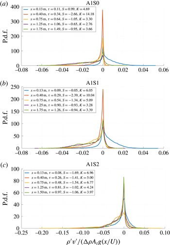
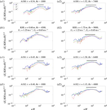
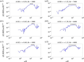
1 Introduction
In the majority of fluid flows, the presence of hydrodynamic instability causes the flow to develop to, or persist in, a turbulent state. Two important hydrodynamic instabilities which often occur together are the buoyancy-driven Rayleigh–Taylor instability (RT instability or RTI) and the shear-driven Kelvin–Helmholtz instability (KH instability or KHI). Together, these instabilities emerge in atmospheric and oceanic flows (Lyons, Panofsky & Wollaston Reference Lyons, Panofsky and Wollaston1964; Browand & Winant Reference Browand and Winant1973; Turner Reference Turner1980; Werne & Fritts Reference Werne and Fritts1999; Kelley et al. Reference Kelley, Chen, Beland, Woodman, Chau and Werne2005), combustion chambers (Nagata & Komori Reference Nagata and Komori2000) and inertial confinement fusion (ICF) targets (Sharp Reference Sharp1984). Much effort has been exerted to understand mixing due to instabilities in the ICF fuel target in order to increase yield and reach ignition (Betti & Hurricane Reference Betti and Hurricane2016). In order to validate models and codes used to predict the outcome of ICF processes, a thorough set of experimental works must be utilized. This paper provides the results of experiments in which the coupled Kelvin–Helmholtz and Rayleigh–Taylor instability (KHRT instability or KHRTI) is studied.
Rayleigh–Taylor instability occurs at the interface of fluids of dissimilar densities. If the pressure gradient (
 $\unicode[STIX]{x0394}p$
) and density gradient (
 $\unicode[STIX]{x0394}\unicode[STIX]{x1D70C}$
) are misaligned such that
 $\unicode[STIX]{x1D735}p\boldsymbol{\cdot }\unicode[STIX]{x1D735}\unicode[STIX]{x1D70C}<0$
, then baroclinic torque is deposited at the interface and small perturbations at the interface begin to grow with time. Often, including in this study, the pressure gradient is the hydrostatic condition caused by gravitational acceleration
 $g$
. The difference in density is quantified by the non-dimensional Atwood number, defined by
 $$\begin{eqnarray}A_{t}=\frac{\unicode[STIX]{x1D70C}_{1}-\unicode[STIX]{x1D70C}_{2}}{\unicode[STIX]{x1D70C}_{1}+\unicode[STIX]{x1D70C}_{2}},\end{eqnarray}$$
where
 $\unicode[STIX]{x1D70C}_{1}$
is the density of the heavier, top fluid and
 $\unicode[STIX]{x1D70C}_{2}$
is the density of the lighter, bottom fluid.
The growth of RTI with multi-mode initial perturbation was delineated in three stages by Youngs (Reference Youngs1984). In the first stage, perturbations grow exponentially according to linear stability theory, with smaller wavelength perturbations growing exponentially faster than large wavelength perturbations (Drazin & Reid Reference Drazin and Reid2004). This analysis was first conducted by Taylor (Reference Taylor1938) and is appropriate at early times when the amplitude of the perturbations are much smaller than their wavelength. Once the amplitude has grown to be approximately half the size of the wavelength, the second stage begins. At that time, small wavelength perturbation growth saturates and slows down (Lewis Reference Lewis1950) while larger wavelength perturbations continue to grow, causing larger structures to appear in the flow and to dominate the development. If large wavelength modes are absent in the initial perturbation, then larger structures appear due to the nonlinear interaction of smaller structures. During this stage, a coherent structure of bubbles and spikes develops. In the third stage, memory of the initial perturbation wavelengths is lost and the flow becomes self-similar. The only remaining length scale of importance is
 $gt^{2}$
, where
 $g$
is gravitational acceleration and
 $t$
is time. In this stage, the total width of the mixed region is given by
 $$\begin{eqnarray}h=2\unicode[STIX]{x1D6FC}A_{t}gt^{2},\end{eqnarray}$$
where
 $\unicode[STIX]{x1D6FC}$
is the RTI growth rate parameter. This result has been arrived at by a variety of techniques, including Lagrangian analysis (Fermi & Neumann Reference Fermi and Neumann1955), modelling of turbulent mix (Birkhoff Reference Birkhoff1955), physical arguments along with linear stability results (Youngs Reference Youngs1984), self-similar analysis of the Navier–Stokes equations (Ristorcelli & Clark Reference Ristorcelli and Clark2004) and a mass flux and energy balance argument (Cook, Cabot & Miller Reference Cook, Cabot and Miller2004). For large density difference (
 $A_{t}>0.2$
), the growth rate parameters for bubble and spike need not be equal (Akula & Ranjan Reference Akula and Ranjan2016).
Kelvin–Helmholtz instability occurs at the shear layer between two fluids with different parallel components of velocities (Chandrasekhar Reference Chandrasekhar1961; Drazin & Reid Reference Drazin and Reid2004). The growth of KHI starts when small perturbations are convected into streams of different fluids, causing an acceleration or deceleration of the perturbation and the development of small spanwise vortices. The instability grows through vortex pairing, the coalescence of neighbouring pairs of vortices to form a larger vortex (Winant & Browand Reference Winant and Browand1974). The self-similar growth of the mixing width is given by
 $$\begin{eqnarray}h=2\unicode[STIX]{x1D6FD}\unicode[STIX]{x0394}Ut,\end{eqnarray}$$
where
 $h$
is the total mixing width,
 $\unicode[STIX]{x1D6FD}$
is the KHI growth rate parameter,
 $\unicode[STIX]{x0394}U$
is the speed difference between the two streams and
 $t$
is time (Pope Reference Pope2000). It is to be noted that at supersonic speed differentials between parallel streams, resultant acoustic dynamics can lead to KHI suppression (Karimi & Girimaji Reference Karimi and Girimaji2016).
When studying the coupled shear–buoyancy instability, it is useful to quantify the relative strength of buoyancy to shear. This can be quantified by the Richardson number
 $Ri$
, defined in the present context by
 $$\begin{eqnarray}Ri=\frac{\displaystyle -g\left(\frac{\unicode[STIX]{x2202}\unicode[STIX]{x1D70C}}{\unicode[STIX]{x2202}y}\right)}{\unicode[STIX]{x1D70C}\displaystyle \left(\frac{\unicode[STIX]{x2202}u}{\unicode[STIX]{x2202}y}\right)^{2}}\sim \frac{-g(\unicode[STIX]{x0394}\unicode[STIX]{x1D70C})h}{\unicode[STIX]{x1D70C}(\unicode[STIX]{x0394}U)^{2}}=\frac{-2gA_{t}h}{(\unicode[STIX]{x0394}U)^{2}},\end{eqnarray}$$
where
 $g$
is the gravitational acceleration,
 $\unicode[STIX]{x1D70C}$
is the density,
 $u$
is the velocity,
 $y$
is the vertical position,
 $\unicode[STIX]{x0394}U$
is the speed difference between the streams,
 $h$
is the total mixing width and
 $A_{t}$
is the Atwood number. In the situation where
 $Ri>0$
, the sign of the density gradient is negative, indicating a stably stratified flow where variations in density can diminish the growth of KHI vortices. The coupled instability, then, can only occur if the value of the Richardson number describing the flow is negative.
Experimental investigations of stably stratified free shear flows have shown that buoyancy causes a decay of turbulence produced by the shear flow. Thorpe (Reference Thorpe1968) used an inclined tube filled with two different liquids to produce a stratified free shear flow. Varying the parameters defining
 $Ri$
on the right-hand side of (1.4), Thorpe (Reference Thorpe1973a
,Reference Thorpe
b
) observed that at
 $Ri\approx 0.33$
, striations started to appear and turbulence began to decay. This
 $Ri$
is referred to as the critical Richardson number. It was observed that the ratio of the velocity interface thickness to the density interface thickness (velocity and density interface thicknesses are defined as the distance between the points in the mixing layer where the velocity and density reach their respective free-stream values) increased with the increased values of the initial Richardson number, i.e.
 $Ri$
based on the initial mixing width at the onset of the instability. The final Richardson number, defined at the centre of the layer based on both velocity and density interface thicknesses, remained constant irrespective of the initial Richardson number after a fixed non-dimensional time from the onset of turbulence. Also, nearly three-quarters of the kinetic energy in the flow was dissipated. After modifying their KHI vortex pairing experimental set-up to study stably stratified free shear layers, Browand & Winant (Reference Browand and Winant1973) noticed the mixing layer profiles collapsed onto a single curve irrespective of the initial density difference between the streams. They concluded that even small amounts of density variation in the flow inhibited vortex pairing and caused the instability to decay. Koop & Browand (Reference Koop and Browand1979) studied the turbulence and flow structure at different Richardson numbers in a stably stratified free shear flow. They observed that at
 $Ri<0.15$
, the vortical structures similar to the plane mixing layer still persisted in their visualization experiments, which was similar to Thorpe’s observation (Thorpe Reference Thorpe1973a
,Reference Thorpe
b
). The flow induced by these vortical structures moved the heavier fluid to the top and the lighter fluid to the bottom. The vortical structures grew in size due to vortex pairing, but they were unable to work against buoyancy and broke down before re-laminarizing into a non-turbulent flow. As the initial Richardson number increased further, the formation of the vortices was not observed and the flow structure was replaced by interfacial waves. Koop & Browand (Reference Koop and Browand1979) showed that the decay of turbulence in the re-laminarizing region is similar to grid turbulence decay. They compared the value of their critical Richardson number with the non-interacting vortex model, and found good agreement with Thorpe’s experiments (Thorpe Reference Thorpe1973a
,Reference Thorpe
b
). They also observed a decreased amount of molecular mixing with increasing values of initial Richardson number after the start of turbulence decay.
Study of unstably stratified free shear flows in which both RTI and KHI are present (KHRT), has been sparse. Lawrence, Browand & Redekopp (Reference Lawrence, Browand and Redekopp1991) performed stability analysis on the coupled instability by solving the Taylor–Goldstein equation with piecewise-linear approximations for the velocity and density profiles. They also conducted experiments with the coupled instability, imaging the flow structure using laser induced fluorescence, and found that the flow initially behaved like a non-stratified shear flow but transitioned into a buoyancy-driven flow. Snider & Andrews (Reference Snider and Andrews1994, Reference Snider and Andrews1996b
) performed experiments in a similar experimental set-up and considered the conditions for transition from shear-dominated to buoyancy-dominated flow. They found transition to occur at
 $Ri$
between
 $-5$
and
 $-10$
. No significant change in the RTI growth rate parameter was detected by adding shear in these experiments. These water channel experiments were limited in the Atwood numbers and velocity differences that could be achieved. Akula, Andrews & Ranjan (Reference Akula, Andrews and Ranjan2013) improved upon the previous experimental work by constructing a gas tunnel which could study a broader range of Atwood numbers and velocity differences. They identified a similar transition from KHI-like to RTI-like instability growth, and determined a transitional Richardson number of
 $-1.5$
to
 $-2.5$
. Hot-wire anemometry was used to measure velocity and density at locations in the flow in order to calculate molecular mixing quantities.
Simulation work on the coupled instability has provided useful insights into the effect of shear on the growth of the buoyancy instability. Snider & Andrews (Reference Snider and Andrews1996a
) used a
 $k$
–
 $\unicode[STIX]{x1D700}$
model to simulate situations similar to those found in their experimental water channel. By considering the form of the self-similar solution, they were able to analytically select values for the constants in the turbulence equations. These simulations matched well with their experimental results, and allowed them to predict that the addition of shear to an RTI flow would reduce the growth rate. The effect of shear in a magnetohydrodynamic flow was simulated by Shumlak & Roderick (Reference Shumlak and Roderick1998), who simulated the
 $z$
-pinch plasma implosion. In this study, the addition of enough shear was found to mitigate and, in some situations, stabilize the buoyancy instability. The high resolution simulations of Olson et al. (Reference Olson, Larsson, Lele and Cook2011) found similar results, and attributed the mitigation to effects in the nonlinear regime. Measures of the peak growth rate parameter of the coupled instability found that it varied non-monotonically with increasing shear. At a certain critical amount of velocity difference between the streams, the growth rate of the RTI could be minimized. An energy budget analysis showed that, at this minimum growth rate, less kinetic energy in the flow was being channelled towards vertical mixing. A non-continuum approach was investigated by Velasco & Muñoz (Reference Velasco and Muñoz2015) who used a multiphase lattice-Boltzmann model to simulate a vertical situation where buoyancy acted parallel to the direction of the shear as opposed to normal to it. The overall effect of the coupled instability on the gold–gas interface of the ICF hohlraum was studied numerically by Vandenboomgaerde, Bonnefille & Gauthier (Reference Vandenboomgaerde, Bonnefille and Gauthier2016). KHI roll-ups were found along the interface of the gold bubble, and during deceleration of the interface, RTI starts to appear. By changing the laser pulse shape and using near-vacuum hohlraums, it was found that the KHI growth could be reduced.
In the present study, the coupled buoyancy–shear instability is experimentally investigated using a multi-layer gas tunnel facility. An effort is made to quantify the Richardson number of transition between KHI-dominated and RTI-dominated flow, and to consider the effect of increasing shear on the overall growth rate of the instability. In addition, while most experiments and simulations have focused on documenting the mixing from the perspective of the density field, the first planar velocity measurements of such a flow are provided to capture the dynamics.
2 Experimental facility and diagnostics
Experiments are performed in the multi-layer gas tunnel facility, an improved version of the two-layer gas tunnel used by Banerjee & Andrews (Reference Banerjee and Andrews2006). Two separated fluid streams, one heavy and one light, are drawn through the facility by a suction fan. Upon entering the test section, the upstream division between the streams is absent and mixing between them begins. Measurements are taken in the test section through visualization techniques, hot-wire anemometry and particle image velocimetry (PIV). The experiment is statistically steady (Snider Reference Snider1994), allowing the measurement of higher-order moments, probability density functions (p.d.f.) and correlations of density and velocity. In such a convective-type system, Taylor’s hypothesis (Taylor Reference Taylor1938; Pope Reference Pope2000) is assumed to relate time
 $t$
from the onset of the instability with
 $x$
using
 $t=x/U$
, where
 $x$
is the streamwise distance from the splitter plate and
 $U$
is the mean velocity of the flow streams. A detailed review of the facility and its improvements is given by Akula (Reference Akula2014) and Akula & Ranjan (Reference Akula and Ranjan2016).
2.1 Gas tunnel facility
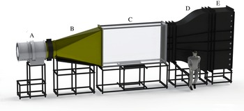
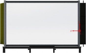
A computer-generated model of the facility is shown in figure 1. All sections except for the fan (section A) and test section (section C) are made of 3.175 mm thick carbon steel. Every section is mounted separately on steel structural tubing stands and casters, allowing sections to be moved and exchanged independently. The entire tunnel is 11.25 m in length. Significant attention is placed in reducing free-stream turbulence in the flow. After construction, the mean velocity variations in the transverse direction and the turbulence intensity value are measured to be
 ${\approx}4\,\%$
and
 ${\approx}0.4\,\%$
of the mean velocity, respectively. Coordinates of the reference system used are shown in figure 2. The origin of the coordinate system is at the splitter plate where both streams begin to mix. The
 $x$
coordinate runs along the direction of flow (streamwise direction), the
 $y$
coordinate runs vertically upward (cross-stream direction) and the
 $z$
direction runs perpendicular to the other two directions into the plane of the figure (spanwise direction).
A computer-generated model of the multi-layer gas tunnel facility. A human model is shown for scale. Flow is from right to left; from section E towards section A.

A computer-generated model of the test section, illustrating the coordinate system.

Flow through the gas tunnel is produced with a 0.80 m diameter suction fan placed at the exit (section A). The rotational speed and blade pitch angle of the fan can be changed to modulate the stream velocities up to maximum speed of
 $20~\text{m}~\text{s}^{-1}$
. Velocity differences between streams are provided by louvers placed at the inlet of the tunnel. Section B is a 2.55 m long square-to-round exit cone which interfaces the rectangular test section (section C) to the fan. To prevent vibrations in the fan from propagating to the rest of the tunnel, the exit cone is not bolted onto the fan, and a gap of approximately 1 mm is left between the two sections. The exit cone includes an access door into the tunnel and a flow straightener is placed in the circular collar.
Measurements are taken inside the test section (section C). Sheets of 12.7 mm thick acrylic are held together with an aluminium frame to form a box of interior dimensions 3.04 m long, 1.83 m tall and 0.61 m wide. The acrylic has a transmittance greater than 99 % in the visible wavelength range. Upstream of the test section, every section is divided into three fluid streams, each separated by a 3.175 mm thick aluminium partition.
Section D is a contraction section connecting the test section to the larger settling section (section E). Near the test section, it contains three steel wire mesh screens carefully selected (Schubauer, Spangenberg & Klebanoff Reference Schubauer, Spangenberg and Klebanoff1950; Loehrke & Nagib Reference Loehrke and Nagib1972; Groth & Johansson Reference Groth and Johansson1988) to reduce the turbulence fluctuation of the streams. The third screen, placed immediately between the partitioned streams and the test section, reduces the effects of the boundary layer formed by the partition.
Gas is injected through gas nozzles mounted inside of the settling section (section E). The nozzles are polyvinyl chloride (PVC) pipes spanning the width of the section that have 6.35 mm holes drilled along their length. Each stream has nine PVC pipes with 12–15 holes per pipe for injecting gas. Two small circulation fans and baffles are installed in the section to promote mixing between the injected gas and air drawn in through the tunnel inlet. In addition, a flow straightener and steel wire mesh screen are placed between the settling section and contraction section (section D). Finally, the inlet of the tunnel is covered by three sets of manual louvers which can be opened and closed to alter the flow rate between streams.
Although the facility is designed and built for experiments with three separate fluid streams, only two are used in the present work. The bottom and middle streams are a helium–air mixture and air, respectively, and the velocity of the top stream is set equal to that of the middle stream. This prevents any shear layer from growing and affecting the interface between the middle and bottom streams. In this paper, the middle stream is referred to as the top stream.
2.2 Visualization
Flow visualization is used to determine the volume fraction profiles of each stream, as well as the bubble and spike mixing widths. The test section is back-lit using an array of light-emitting diode (LED) panels covering an area
 $3.05~\text{m}\times 1.83~\text{m}$
. A large sheet of matte acetate paper is placed between the light panels and the test section to ensure diffuse and uniform lighting of the flow. One fluid stream is seeded with fog particles composed of condensed ethylene glycol. The fog is four times more dense than air and is injected at the rate of
 $2~\text{g}~\text{s}^{-1}$
. This affects the stream density, changing the Atwood number by
 ${\approx}3\,\%$
at an Atwood number of 0.07 (Akula Reference Akula2014). As the Atwood number approaches unity and the difference between fluid densities increases, the effect of fog injection in the stream decreases. The fog is produced by a fog generator and pushed towards the louvers using a ventilation fan. The fog is drawn into the air stream due to the suction drawn through the tunnel, and is mixed with the air using a series of baffles and mixing fans placed in the settling section.
The injected gas acts as a thin light-extincting medium, and the absorption of light due to the presence of the fog is linearly proportional to the volume fraction of fog (as approximated from Beer–Lambert’s law) (Akula et al. Reference Akula, Andrews and Ranjan2013). Images of the flow are then collected and pixel intensity is converted to volume fraction using a wedge calibration technique (Banerjee & Andrews Reference Banerjee and Andrews2006).
Images are collected at a rate of 60–300 images per minute depending on the velocity and Atwood number of the experiment. Approximately 200 large-scale structures per averaging and thus 200 images are needed to obtain statistically convergent data on the mixing width (Banerjee & Andrews Reference Banerjee and Andrews2006). In experiments with larger Atwood number, the velocity of the flow is increased, and more structures are convected in the same amount of time as in an experiment with smaller Atwood number. Thus, for larger Atwood number experiments, a larger frame rate is used. The images are captured with a Nikon® D90/D4 camera with an
 $f8$
aperture, ISO sensitivity of 100, and shutter speed of
 $1/100$
s. The images are ensemble averaged and processed through a background subtraction technique to remove non-uniformities (Banerjee & Andrews Reference Banerjee and Andrews2006). The MATLAB® contour function is used to find the volume fraction contours corresponding to the spike and bubble mixing width. The signal from the fogged stream is small at the edge of the mixing layer and it is difficult to obtain the required (say, 95 %) volume fraction point location. Therefore, each experiment is repeated two times with fog particles injected in a different stream each time. When the bottom stream is injected with fog, the bubble height is obtained and injecting into the top stream gives the spike height.
2.3 Particle image velocimetry
In the past three decades, PIV has become an increasingly powerful and important technique for experimental fluid mechanics. In conventional box-type experimental set-ups studying fluid instabilities, the implementation of PIV is difficult due to particle seeding issues and short experiment durations. However, the statistically steady nature of the present experimental facility has lent itself to PIV measurement. A detailed validation of the technique in this facility is presented elsewhere (Akula Reference Akula2014; Akula & Ranjan Reference Akula and Ranjan2016).
There are three fundamental components to a PIV system: particle seeding, particle illumination and image capture. For this flow, both streams are injected with oil particles produced by a Pea Soup Phantom PS33 H1 180 model fog machine. The size of the particles is between 0.2 and
 $1~\unicode[STIX]{x03BC}\text{m}$
. The particles are illuminated by a Litron LPU 550 dual-head laser with a 120 mJ pulse and maximum pulse frequency of 15 Hz. The laser sheet is oriented in the
 $x$
–
 $y$
plane in the test section and formed using a converging lens (focal length 1000 mm), a cylindrical diverging lens (focal length
 $-15/-12.7$
mm) and a reflecting mirror (50.8 mm diameter). The repetition rate of laser 1 is controlled by triggering the laser 1 flash lamp via a National Instruments PCIe-6321 DAQ card. Internal timing in the laser triggers the laser 1 Q-switch after a time of approximately
 $80~\unicode[STIX]{x03BC}\text{s}$
. The signal from the laser 1 Q-switch is also sent to a Berkeley Nucleonics Corporation (BNC) model 555 pulse delay generator which triggers the laser 2 flash lamp and Q-switch. Images are captured with a TSI 630157 dual-frame charge-coupled device camera, equipped with 50 mm focal length Nikon lenses. The cameras are controlled through the TSI INSIGHT4G® software, and data from the cameras are collected by a frame grabber installed on the motherboard of the acquisition computer.
One thousand two hundred image pairs are collected at a rate of 15 Hz for all experiments. In order to obtain a statistically steady value for turbulence quantities, at least 400 images must be collected, past which values vary by less than 3 %. Thus, the 1200 collected image pairs at each station represent a statistically steady flow field.
The PIV processing method is performed through the TSI INSIGHT4G® software by searching for the peak of the cross-correlation between windows around points of the image. A signal to noise ratio (SNR) of 1.5 must be achieved in a given window for a data point to be collected at that location. In most cases, 95 % of data points successfully pass the SNR test, with the majority of failures being at the edges of the image.
2.4 Hot-wire anemometry
The simultaneous measurement of density and velocity are necessary to quantify certain important turbulence quantities. This is accomplished through simultaneous three-wire and cold-wire anemometry (S3WCA) analyses detailed by Kraft (Reference Kraft2008). This method is based on the earlier efforts of Hishida & Nagano (Reference Hishida and Nagano1978) and Vukoslavc̆ević, Radulović & Wallace (Reference Vukoslavc̆ević, Radulović and Wallace2005) to perform simultaneous temperature and velocity measurements with hot-wire analysis. In this technique, temperature is used as a marker for density by slightly heating one stream. As the Lewis number of the fluids used in the experiment is nearly unity, thermal and molecular diffusivity are similar in magnitude and the measured temperature can be correlated to volume fraction. Heat guns aimed at the heated stream raise the temperature by approximately
 $2\,^{\circ }\text{C}$
. Due to the low Atwood numbers used in the experiments, any larger temperature rise would cause larger uncertainty in Atwood number. The temperature of both streams is measured in the centre of each stream immediately after passing the final steel wire mesh screen by the use of K-type thermocouples.
Two probes are placed in the flow in close proximity to one another. The first is a Dantec Dynamics 55P91 three-wire probe which is used to measure velocity in three component directions. Each wire of the probe is held at
 $250\,^{\circ }\text{C}$
by a Dantec Dynamics MiniCTA 54T42 constant temperature anemometer with an overheat ratio of 0.83. The other is a cold-wire probe used to measure temperature. Together, the probes take simultaneous measurements with a spatial resolution of 6 mm. The sampling frequency is 1000 Hz.
The cold-wire probe senses fluid temperature independent of the concentration of the flow. Combined with the temperature of each unmixed stream, the concentration of fluid can be obtained after performing an energy balance (Kraft, Banerjee & Andrews Reference Kraft, Banerjee and Andrews2009). The resulting equations for concentration by mass and by volume are
 $$\begin{eqnarray}\displaystyle & \displaystyle f_{m,2}(t)=\left[1+\frac{c_{p,2}}{c_{p,1}}\frac{T_{2}(t)-T_{mix}(t)}{T_{mix}(t)-T_{2}(t)}\right]^{-1}, & \displaystyle\end{eqnarray}$$
 $$\begin{eqnarray}\displaystyle & \displaystyle f_{v,2}(t)=\frac{\unicode[STIX]{x1D70C}_{1}}{\unicode[STIX]{x1D70C}_{1}-\unicode[STIX]{x1D70C}_{2}+\unicode[STIX]{x1D70C}_{2}/f_{m,2}(t)}, & \displaystyle\end{eqnarray}$$
where a subscript 1 refers to the top stream, subscript 2 refers to the bottom stream,
 $f_{m,i}$
is the mass fraction of stream
 $i$
,
 $f_{v,i}$
is the volume fraction of stream
 $i$
,
 $c_{p}$
is the specific heat,
 $T$
is the temperature and
 $\unicode[STIX]{x1D70C}$
is the density.
3 Results and discussion
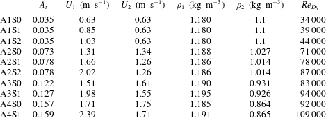
Parameters for different experimental cases are summarized in table 1. Cases are named as A
 $n$
S
 $m$
where A
 $n$
represents experiments at the same
 $A_{t}$
; increasing values of
 $n$
indicate experiments at higher
 $A_{t}$
. For experiments at the same
 $A_{t}$
, S
 $m$
represents experiments with different amounts of shear; increasing values of
 $m$
indicate experiments with higher shear, with S0 being RTI only (no shear) experiments.
 $Re_{D_{h}}=UD_{h}/\unicode[STIX]{x1D708}_{mix}$
is the Reynolds number based on the hydraulic diameter
 $D_{h}$
of the test section, where
 $U=(U_{1}+U_{2})/2$
is the mean convective speed and
 $\unicode[STIX]{x1D708}_{mix}$
is obtained as per Wilke (Reference Wilke1950).
 $D_{h}=4A_{c}/P$
where
 $A_{c}$
is the cross-sectional area of the test section and
 $P$
is the cross-sectional wetted perimeter.
Parameters for different sets of experiments performed in the present work (subscripts 1 and 2 refer to top and bottom streams, respectively). Velocities reported have an uncertainty of 4 %.
 $\unicode[STIX]{x1D70C}_{1}$
has an uncertainty of 0.15 % and
 $\unicode[STIX]{x1D70C}_{2}$
has an uncertainty of 1.7 %. Atwood numbers have an uncertainty of 11 %.
 $Re_{D_{h}}$
is the Reynolds number based on the hydraulic diameter of the test section.

Experiments A1S0, A1S1 and A1S2 were performed in the two-layer gas tunnel facility (Akula et al.
Reference Akula, Andrews and Ranjan2013; Akula Reference Akula2014), and all other cases were performed in the multi-layer gas tunnel facility. Visualization and S3WCA are used to measure the mixing widths as well as instantaneous velocity and density for A1S0, A1S1 and A1S2. In addition to these two diagnostics, two-dimensional (2-D) PIV measurements acquired the flow field information of the streamwise (
 $u$
) and cross-stream (
 $v$
) velocity components for all other cases (A2, A3 and A4). Helium is injected into the bottom stream to provide the density difference between the streams. Before the start of the experiment, the velocity of the bottom stream (
 $U_{bot}$
or
 $U_{2}$
) is intentionally kept smaller than the indicated value in table 1 to compensate for the velocity increase due to the injection of helium. The velocity increase due to helium and air mixture injection is estimated a priori by Amagat’s law (Moran & Shapiro Reference Moran and Shapiro2000) and the actual measurements agree with the Amagat’s law estimation. The density of the top stream,
 $\unicode[STIX]{x1D70C}_{1}$
, is assumed to be that of air at the temperature measured by a thermocouple in the stream. Amagat’s law, as formulated (Akula et al.
Reference Akula, Andrews and Ranjan2013) by
 $$\begin{eqnarray}\unicode[STIX]{x1D70C}_{bot}^{mix}=\unicode[STIX]{x1D70C}_{2}=\unicode[STIX]{x1D70C}_{air}+\frac{{\dot{m}}_{He}}{U_{2}A}\left[1-\frac{\unicode[STIX]{x1D70C}_{air}}{\unicode[STIX]{x1D70C}_{He}}\right]\end{eqnarray}$$
is used to calculate the density of the bottom stream (
 $\unicode[STIX]{x1D70C}_{bot}^{mix}$
or
 $\unicode[STIX]{x1D70C}_{2}$
) based on the densities of air and helium at the stream temperature (
 $\unicode[STIX]{x1D70C}_{air}$
and
 $\unicode[STIX]{x1D70C}_{He}$
, respectively) and the known mass flow rate of helium (
 ${\dot{m}}_{He}$
).
 $A$
in (3.1) is the cross-sectional area of the bottom stream;
 $\unicode[STIX]{x1D70C}_{1}$
and
 $\unicode[STIX]{x1D70C}_{2}$
are used to calculate the Atwood number (1.1).
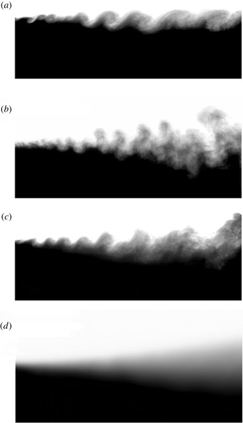
Typical flow visualization images (flow from left to right): (a) shear only experiment with air,
 $U_{1}=0.85~\text{m}~\text{s}^{-1}$
and
 $U_{2}=0.60~\text{m}~\text{s}^{-1}$
(image courtesy of Akula et al. (Reference Akula, Andrews and Ranjan2013)). (b) Instantaneous image from case A1S0. (c) Instantaneous image from case A1S1 (image courtesy of Akula et al. (Reference Akula, Andrews and Ranjan2013)). (d) Mixing width evolution after ensemble averaging of instantaneous images from case A1S1. These images correspond to a visualization window of approximately
 $150~\text{cm}\times 70~\text{cm}$
in size.

Volume fraction
 $f_{v,2}$
and corresponding mean fluid density profiles
 $\overline{\unicode[STIX]{x1D70C}}(y)$
for different KHRT cases.

3.1 Mixing growth and phenomenology
3.1.1 Flow structures
Typical instantaneous visualization images after background subtraction are shown in figure 3(a–c). Panel (a) is taken from a pure KHI case, and the spanwise vortical structures which are characteristic of free shear flows are clearly seen. Panel (b) is taken from a pure RTI case (A1S0). Unlike KHI, RTI produces vertical plumes of rising bubbles and falling spikes, and the corresponding mushroom-like structures observed develop due to shear at the interface between these opposing plumes. For the coupled KHRT case (A1S1), shown in panel (c), the flow is dominated by KHI-type vortical structures in initial stages which are stretched and diffused by vertical RTI plumes in later stages. This trend is attributed to the competing KHI and RTI growth rates at different stages of the flow (Akula et al. Reference Akula, Andrews and Ranjan2013).
The image shown in figure 3(d) is obtained by ensemble averaging a large set of images similar to the one in figure 3(c). The ensemble-averaged image is used to find the volume fraction contours corresponding to the upper and lower edges of the mixing width (also referred to as the mixing height). For the present study, 5 % and 95 % volume fraction points (with respect to bottom stream fluid) are chosen as the criterion to locate these upper and lower edges, respectively, in order to calculate the mixing width. This criterion was used in our previous work (Akula et al.
Reference Akula, Andrews and Ranjan2013; Akula Reference Akula2014; Akula & Ranjan Reference Akula and Ranjan2016) and its use was also justified by Snider & Andrews (Reference Snider and Andrews1994). To put this into perspective, for the case A1S2 at a distance of 1 m from the splitter plate, a 5–95 % criterion gives a mixing width of 21.48 cm, compared to a mixing width of 18.53 cm obtained using a 10–90 % criterion, and a mixing width of 25.73 cm obtained using a 1–99 % criterion. An integral measure of mixing width was also considered, following the work of Snider & Andrews (Reference Snider and Andrews1994), with
 $h=6\int f_{v,1}f_{v,2}\,\text{d}y$
. For the same case and streamwise location, a mixing width of 26.03 cm was found.
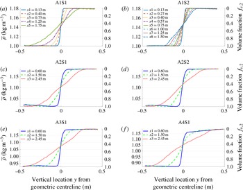
The volume fraction profiles (
 $f_{v,2}$
) and corresponding mean fluid density profiles (
 $\overline{\unicode[STIX]{x1D70C}}(y)$
) obtained at different streamwise location
 $x$
for different KHRT cases are shown in figure 4;
 $f_{v,2}$
and
 $\overline{\unicode[STIX]{x1D70C}}(y)$
are related by
 $\overline{\unicode[STIX]{x1D70C}}=\unicode[STIX]{x1D70C}_{1}-(f_{v,2}\unicode[STIX]{x0394}\unicode[STIX]{x1D70C})$
, where
 $\unicode[STIX]{x0394}\unicode[STIX]{x1D70C}=\unicode[STIX]{x1D70C}_{1}-\unicode[STIX]{x1D70C}_{2}$
is the density difference between the top and bottom streams. Relating volume fraction and mean fluid density is based on the assumption that volume fractions obtained from visualization describe the extent of molecular mixing in the flow (Dimotakis Reference Dimotakis1991). The volume fraction profiles across the mixing layer are expected to be linear in the core and vary like an error function distribution at the edges of the mixing layer (Dimonte & Schneider Reference Dimonte and Schneider2000; Banerjee, Gore & Andrews Reference Banerjee, Gore and Andrews2010a
). The same is observed for the profiles in figure 4. These volume fraction and mean density profiles are later used to derive vertical gradients of mean density across the mixing layer, required for Richardson number calculations. As seen from figure 4, the point of volume fraction
 ${\approx}0.5$
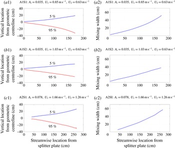
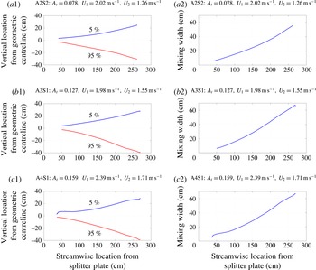
falls below the geometric centreline with increasing streamwise distance, which is typical of free shear flows (Pope Reference Pope2000). It indicates the shift of the mixing centreline (i.e. 50 % volume fraction contour) below the geometric centreline towards the slow moving fluid stream. The 5 % and 95 % volume fraction contours of the bottom stream are shown in the left columns of figures 5 and 6, and the total mixing widths (
 $h_{t}$
or simply
 $h$
) are shown in the right columns.
Upper (
 $f_{v,2}=0.05$
) and lower (
 $f_{v,2}=0.95$
) edges of the mixing width, and the total mixing width for different experimental cases.

Upper (
 $f_{v,2}=0.05$
) and lower (
 $f_{v,2}=0.95$
) edges of the mixing width and the total mixing width for different experimental cases.

3.1.2 Mixing widths and growth rate parameters
In the self-similar stage, the mixing width grows linearly with time for KHI (
 ${\sim}\unicode[STIX]{x0394}Ut\sim (\unicode[STIX]{x0394}U/U)x$
) (Brown & Roshko Reference Brown and Roshko1974; Winant & Browand Reference Winant and Browand1974; Bell & Mehta Reference Bell and Mehta1990; Dimotakis Reference Dimotakis1991) and quadratically with time for RTI (
 ${\sim}A_{t}gt^{2}\sim A_{t}g(x/U)^{2}$
) (Birkhoff Reference Birkhoff1955; Fermi & Neumann Reference Fermi and Neumann1955; Youngs Reference Youngs1984; Cherfils & Mikaelian Reference Cherfils and Mikaelian1996; Cook et al.
Reference Cook, Cabot and Miller2004; Ristorcelli & Clark Reference Ristorcelli and Clark2004). Details on growth rate parameters and their calculations from experiments with both two-layer and multi-layer gas tunnels for KHI and RTI cases can be found in Akula (Reference Akula2014).
For the coupled instability, it was proposed by Akula et al. (Reference Akula, Andrews and Ranjan2013) that the total mixing-layer width would grow at a rate predicted by
 $$\begin{eqnarray}\displaystyle h & = & \displaystyle 2\unicode[STIX]{x1D6FD}\unicode[STIX]{x0394}Ut+2\unicode[STIX]{x1D6FC}_{khrt}A_{t}gt^{2},\quad t>t_{tr}\nonumber\\ \displaystyle & = & \displaystyle 2\unicode[STIX]{x1D6FD}\unicode[STIX]{x0394}U\left(\frac{x}{U}\right)+2\unicode[STIX]{x1D6FC}_{khrt}A_{t}g\left(\frac{x}{U}\right)^{2},\quad x>x_{tr},\end{eqnarray}$$
which combines the self-similar mixing width growth equations for KHI and RTI. The equation holds after the flow has transitioned into the buoyancy-dominated regime (
 $t>t_{tr}$
or equivalently,
 $x>x_{tr}$
).
 $\unicode[STIX]{x1D6FD}$
is the growth rate parameter for a KHI case with identical mean convective speed
 $U=(U_{1}+U_{2})/2$
and velocity difference
 $\unicode[STIX]{x0394}U=U_{1}-U_{2}$
, but without any density difference, and
 $t=x/U$
is the development time where
 $x$
is streamwise distance from the splitter plate. For velocity ratios
 $U/\unicode[STIX]{x0394}U<4$
,
 $\unicode[STIX]{x1D6FD}\approx 0.15{-}0.19$
(Akula Reference Akula2014) and closely resembles previous estimates as in Brown & Roshko (Reference Brown and Roshko1974). After substituting for
 $\unicode[STIX]{x1D6FD}$
,
 $\unicode[STIX]{x1D6FC}_{khrt}$
is calculated using the method of Ristorcelli & Clark (Reference Ristorcelli and Clark2004) (RC) and the virtual-origin (VO) method (Snider & Andrews Reference Snider and Andrews1994). At late times, the quadratic RTI term in (3.2) dominates and the instability shows parabolic growth. The same trend can also be seen for mixing width evolutions shown in figures 5 and 6. This transition from shear to buoyancy dominance in KHRT flows will later be quantified using the transitional Richardson number.
The
 $\unicode[STIX]{x1D6FC}_{khrt}$
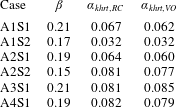
values obtained for different KHRT cases using both RC and VO methods are shown in table 2. Except for the A1S2 case, all cases have
 $\unicode[STIX]{x1D6FC}_{khrt}$
values of 0.064–0.082. For the A1S2 case, the transition to the RTI regime occurs near the end of the tunnel. If the mixing layer has not transitioned into RTI-like behaviour,
 $\unicode[STIX]{x1D6FC}_{khrt}$
will be less than the pure RTI
 $\unicode[STIX]{x1D6FC}$
value. It is interesting to note that, irrespective of the amount of shear or buoyancy present, the measured
 $\unicode[STIX]{x1D6FC}_{khrt}$
value is in a small range and is within the range of values typically recorded for RTI (Snider & Andrews Reference Snider and Andrews1994; Ramaprabhu & Andrews Reference Ramaprabhu and Andrews2004; Mueschke, Andrews & Schilling Reference Mueschke, Andrews and Schilling2006; Mueschke & Schilling Reference Mueschke and Schilling2009a
). This statement is true only after the mixing layer has transitioned into RTI-like behaviour. This transition criterion is discussed in the next section. It is to be noted that the flow transitions into a buoyancy-dominated regime which does not immediately become self-similar until later (further downstream) in the flow. Thus, equation (3.2) need not represent a self-similar flow although its individual terms represent self-similar KHI and RTI growth.
Growth rate parameters:
 $\unicode[STIX]{x1D6FC}_{khrt}$
calculated for different cases using both RC and VO methods, taking
 $\unicode[STIX]{x1D6FD}$
from the shear only experiments at the same set of parameters.

3.1.3 Transition from shear-dominated to buoyancy-dominated flow
From the visualization study of the coupled instability experiments, it is clear that the mixing layer exhibits KHI-like behaviour at earlier times and transitions into RTI-like behaviour at later times. It is important to quantify this transition point for different cases and determine any criterion for transition. This criterion can be used to predict the mixing growth rate as explained previously in § 3.1.2. It could also be used to switch from shear only to coupled shear–buoyancy physics in turbulence models and simulations.
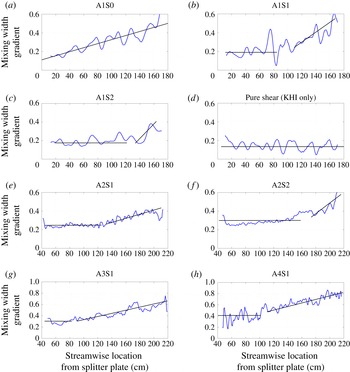
Because the shear mixing width grows linearly with time, the gradient of the mixing width with respect to time is a constant. Meanwhile, the RTI mixing width grows quadratically with time, yielding a gradient with respect to time which increases linearly. For the coupled instability, then, there should exist a streamwise region (time range after coordinate transformation) over which the plot of the mixing width gradient shifts from a constant value to linear growth. The location of this region is identified as the transition location,
 $x_{tr}$
, with corresponding transition time,
 $t_{tr}=x_{tr}/U$
. The mixing width gradient is calculated by a moving window technique (Akula et al.
Reference Akula, Andrews and Ranjan2013), in which two windows of 100 pixels in size are placed side by side and traversed downstream. Mixing width values are averaged in each window and the gradient is calculated using the averaged values through a finite difference approximation.
Mixing width gradient variation along the test section for different experimental cases.

Figure 7 shows the mixing width gradients (non-dimensional) for different KHRT cases, along with one pure RTI case (panel (a)) and one pure KHI case (panel (d)). Each panel shows the actual mixing width gradient, and the corresponding trend marked using straight lines. The oscillatory behaviour is due to small fluctuations in the mixing width information obtained from the image analysis (Akula et al.
Reference Akula, Andrews and Ranjan2013). The approximate location of the change in trend from constant to linearly increasing is used to calculate the transition location. These transition locations are also verified using a least squares fit of a zeroth-degree polynomial and a first-degree polynomial, and an uncertainty of
 $\pm 10$
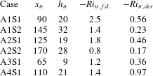
cm is associated with these locations. These transition locations and corresponding mixing widths at these locations are tabulated in table 3. As expected, at similar
 $A_{t}$
, increasing shear delays the transition from KHI-like to RTI-like behaviour. Also, comparing cases with similar values of
 $\unicode[STIX]{x0394}U$
, such as
 $\{\text{A1S2},\text{A2S1},\text{A3S1}\}$
or
 $\{\text{A2S2},\text{A4S1}\}$
, increasing
 $A_{t}$
causes early transition.
Streamwise location of transition from KHI-dominance to RTI-dominance (
 $x_{tr}$
, cm), the total mixing width (
 $h_{tr}$
, cm) at transition location, and the transitional Richardson numbers (
 $Ri_{tr}$
) for different KHRT cases.

The Richardson number
 $Ri$
(1.4) quantifies the competition between buoyancy and shear production of turbulent kinetic energy in atmospheric and oceanic flows (Lyons et al.
Reference Lyons, Panofsky and Wollaston1964; Werne & Fritts Reference Werne and Fritts1999; Kelley et al.
Reference Kelley, Chen, Beland, Woodman, Chau and Werne2005). For the present case, the definition of
 $Ri$
in derivative form (henceforth, referred to as
 $Ri_{der}$
) is given by
 $$\begin{eqnarray}Ri_{der}=\frac{\displaystyle -g\left(\frac{\unicode[STIX]{x2202}\unicode[STIX]{x1D70C}}{\unicode[STIX]{x2202}y}\right)}{\displaystyle \unicode[STIX]{x1D70C}\left(\frac{\unicode[STIX]{x2202}u}{\unicode[STIX]{x2202}y}\right)^{2}}.\end{eqnarray}$$
Approximating the derivatives in (3.3) with their finite difference forms (
 $\unicode[STIX]{x2202}\unicode[STIX]{x1D70C}/\unicode[STIX]{x2202}y\approx \unicode[STIX]{x0394}\unicode[STIX]{x1D70C}/h$
,
 $\unicode[STIX]{x2202}u/\unicode[STIX]{x2202}y\approx \unicode[STIX]{x0394}U/h$
,
 $\unicode[STIX]{x0394}\unicode[STIX]{x1D70C}=\unicode[STIX]{x1D70C}_{1}-\unicode[STIX]{x1D70C}_{2}$
) and using the definition of
 $A_{t}$
, we arrive at the finite difference form of
 $Ri$
(henceforth, referred to as
 $Ri_{f.d.}$
), given by
 $$\begin{eqnarray}Ri_{f.d.}=\frac{-2gA_{t}h}{(\unicode[STIX]{x0394}U)^{2}}.\end{eqnarray}$$
The dependence of coupled shear–buoyancy transition on
 $Ri_{f.d.}$
has been discussed by Snider & Andrews (Reference Snider and Andrews1994, Reference Snider and Andrews1996b
), Akula et al. (Reference Akula, Andrews and Ranjan2013) and Akula (Reference Akula2014). Note that for a given set of experimental parameters,
 $Ri_{f.d.}$
is solely dependent on the mixing width,
 $h$
, itself only varying with streamwise location,
 $x$
.
 $Ri_{f.d.}$
can thus be treated as a non-dimensional measure of the mixing width and can be used to find a transition Richardson number,
 $Ri_{tr}$
, at the streamwise location of transition.
In going from
 $Ri_{der}$
to
 $Ri_{f.d.}$
, one generally assumes the mixing width for density,
 $h_{den}$
, and for velocity,
 $h_{vel}$
, are the same, which need not always be true. The two mixing widths are also referred to as density and velocity interface thicknesses. Though the two mixing widths are expected to scale proportionally (Dimotakis Reference Dimotakis1991) and the definition of
 $h$
should not affect the overall Richardson number dependence of the mixing width, the actual magnitude of
 $Ri_{tr}$
does depend on the definition of
 $h$
and holds some physical importance.
The mixing width
 $h$
that has been referred so far in this paper is based on visualization (
 $h_{viz}$
) and closely resembles the mixing width based on mean density variation (
 $h_{den}$
) of molecularly mixed fluid (Dimotakis Reference Dimotakis1991) (i.e.
 $h\approx h_{viz}\approx h_{den}$
). The mixing width based on velocity (
 $h_{vel}$
) is often defined (Dimotakis Reference Dimotakis1991) in terms of the mean streamwise velocity profile
 $\overline{U}(y)$
as
 $$\begin{eqnarray}h_{vel}=\frac{\unicode[STIX]{x0394}U}{\displaystyle \left(\frac{\text{d}\overline{U}(y)}{\text{d}y}\right)_{max}}.\end{eqnarray}$$
The mixing width
 $h_{vel}$
is also referred to as the vorticity (or maximum slope) thickness and is found to be approximately half of
 $h_{viz}$
for experiments with gases (Dimotakis Reference Dimotakis1991). This is discussed later in § 3.1.4 in greater detail. Because the difference between the two mixing widths is not accounted for in the calculation of
 $Ri_{f.d.}$
, its magnitude should be approximately four times larger than that of
 $Ri_{der}$
. In the present work, density and velocity gradients measured across the mixing layer are used with the definition of
 $Ri_{der}$
to determine transitional Richardson number,
 $Ri_{tr,der}$
(velocity gradients are calculated from
 $\overline{U}(y)$
profiles in § 3.2). These are compared with the transitional Richardson numbers (
 $Ri_{tr,f.d.}$
) obtained using (3.4) (Akula Reference Akula2014). Both
 $Ri_{tr}$
values are obtained at transition locations, and are reported in table 3. The magnitude of
 $Ri_{tr,der}$
is less than unity for all the KHRT cases. Except for A4S1,
 $Ri_{tr,der}$
and
 $Ri_{tr,f.d.}$
for all other cases are approximately related by a factor around 4, which can be attributed to the previously discussed scaling between
 $h_{viz}$
and
 $h_{vel}$
. The discrepancy for case A4S1 could be due to using only a single PIV camera during velocity measurement which may have failed to capture the entire velocity mixing width. At
 $|Ri|\approx 1$
, flows are considered to be buoyancy dominated (Lyons et al.
Reference Lyons, Panofsky and Wollaston1964) and thus, transition should occur at
 $|Ri|<1$
when buoyancy and shear are of comparable strength. The magnitudes of
 $Ri_{tr,der}$
obtained here are in accordance with this prediction.
As discussed in § 1, for stably stratified free shear flows, Thorpe (Reference Thorpe1968, Reference Thorpe1973a
,Reference Thorpe
b
, Reference Thorpe1971) and Browand & Winant (Reference Browand and Winant1973) observed the shear layer to transition to a region of almost constant thickness, and they associated a critical Richardson number with this thickness. This observation was one of the early motivations to investigate the dependence of KH to RT transition on some critical Richardson number. Snider & Andrews (Reference Snider and Andrews1994) found KH to RT transition to occur at
 $Ri_{f.d.}=-5$
to
 $-10$
at
 $A_{t}$
of the order of
 $10^{-3}$
. Akula et al. (Reference Akula, Andrews and Ranjan2013) found
 $Ri_{tr}$
to be in the range of
 $-1.5$
to
 $-2.5$
in
 $A_{t}=0.035$
experiments. D. M. Israel (Personal communication 2014, Encyclopedia of analytic and approximate analytic solutions to the Boussinesq mixing-layer, Los Alamos National Laboratory) shows analytically that if shear scaling (
 ${\sim}t$
) is assumed at early time and buoyant scaling (
 ${\sim}t^{2}$
) at late time, a piecewise solution for
 $h$
indicates an instantaneous switch from shear to buoyancy self-similar behaviour at some critical
 $Ri$
. He suggests the need for turbulence modelling to remove the unphysical sharp transition. Using a simple one equation model (Tennekes & Lumley Reference Tennekes and Lumley1972; Ristorcelli & Clark Reference Ristorcelli and Clark2004), Israel (2014) shows that the temporal evolution of KHRT mixing width is only dependent on the non-dimensional mixing width or associated
 $Ri$
. Thus, the KH to RT transition should be quantifiable in terms of
 $Ri$
. But this
 $Ri_{tr}$
need not just be a single number, and may show a spread in values or narrow range, as observed for stably stratified free shear flows (Thorpe Reference Thorpe1971; Browand & Winant Reference Browand and Winant1973).
One of the most remarkable observations about
 $Ri_{tr}$
obtained in our experiments is that their magnitudes closely resemble the transitional layer Richardson number (
 $R_{iL}$
) at which Thorpe (Reference Thorpe1971) observed ‘domination of striated structures over rounded billows’ in a stably stratified free shear layer. As per Thorpe (Reference Thorpe1971), the shear-layer thickness became constant at
 $Ri\approx 0.4$
, indicating decay of turbulence in stably stratified free shear flow. The definition of Richardson number used by Thorpe (Reference Thorpe1971), though a finite difference one, uses the Brunt–Väisälä frequency (AMS 2017) which could be related to the density gradient in
 $Ri_{der}$
or
 $Ri_{f.d.}$
definitions. Different studies (Taylor Reference Taylor1931; Lyons et al.
Reference Lyons, Panofsky and Wollaston1964; Browand & Winant Reference Browand and Winant1973; Werne & Fritts Reference Werne and Fritts1999; Kelley et al.
Reference Kelley, Chen, Beland, Woodman, Chau and Werne2005; AMS 2017) have found this critical or transitional
 $Ri$
for stably stratified free shear flows, and the magnitudes there too vary between 0.2 and 1.0, the range which has been observed with present KHRT experiments and the
 $Ri_{tr,der}$
definition. The similarity in
 $Ri_{tr}$
(with opposite signs) between stably and unstably stratified free shear flows may not be a mere coincidence, and could indicate a universal or analogous role of buoyancy in affecting flows which are initially shear dominated. For stably stratified flows, density difference leads to decay of turbulence while for unstable stratification, it enhances turbulence. More studies, encompassing wider ranges of velocity and density ratios, are required before anything can be conclusively said about this. If such an analogy exists, this will be of immense significance for atmospheric and oceanic fluid mechanics where many studies exist for stable stratification and results from these studies can be extended to unstably stratified situations. Also, the KH to RT transition criterion based on
 $Ri_{tr}$
should be useful for numerical hydrodynamic solvers to decide between suitable KHI related and RTI related turbulence models.
Evolution of visualization and velocity-based mixing widths for A1S2 case.

3.1.4 Evolution of mass and momentum mixing layers
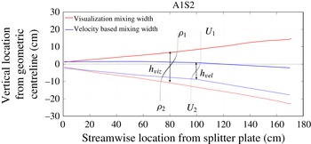
It has been mentioned previously in § 3.1.1 that the mixing centreline falls below the geometric centreline. Also, as mentioned in § 3.1.3, the mixing width obtained from visualization appropriately gives the extent of density-based mixing width or mass mixing-layer thickness (
 $h\approx h_{viz}\approx h_{den}$
), and the velocity-based mixing width or momentum mixing-layer thickness
 $h_{vel}$
is found to be approximately half of
 $h_{viz}$
for experiments with gases (Dimotakis Reference Dimotakis1991). Mass diffusion is expected to be more prominent than momentum diffusion due to a gaseous Schmidt number
 $Sc\approx 0.7$
which is less than unity. However, this value of
 $Sc$
is not small enough to cause the momentum diffusion layer to be half as thick as the mass diffusion layer. Other factors such as fluid entrainment due to turbulent shear and buoyancy (for unstable stratification) also contribute to mass transport in addition to diffusion, thickening the mass mixing layer. This is also the reason why such a flow feature is referred to as a mixing layer, not a diffusion layer.
For the present KHRT experiments, mean density profiles (figure 4) and mean streamwise velocity profiles
 $\overline{U}(y)$
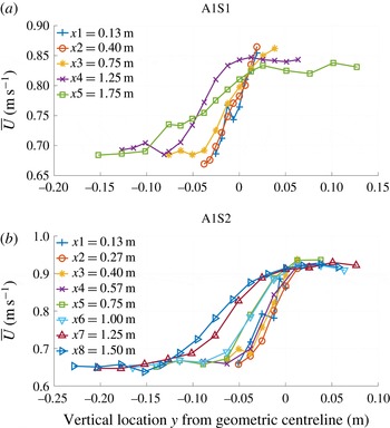
(figure 9), obtained at different streamwise locations can be interpolated to give the simultaneous evolution of visualization/density-based and velocity-based mixing widths. Velocity-based mixing widths are defined similar to visualization mixing widths, approximately based on 5 %–95 % thresholds. Such a mixing-layer thickness is close in magnitude to the vorticity (or maximum slope) thickness discussed earlier. The evolution of mixing widths for case A1S2 is shown in figure 8. While the density mixing layer shifts only slightly below the geometric centreline, the velocity mixing layer shifts dramatically; at late times, even the upper edge of the velocity mixing layer falls below the geometric centreline. This large fall in the velocity mixing layer can be attributed to the tendency of shear layers to spread preferentially into the low-speed stream (Pope Reference Pope2000), and the relatively higher momentum of the top stream (greater speed and density). Such an asymmetry is more pronounced for KHRT than KHI. Another way to understand this difference in the evolution of two mixing widths is to compare mean density and streamwise velocity profiles (i.e. compare panels (b) of figures 4 and 9). The mean density profiles show a degree of symmetry about a central cross-over point, but no such prominent cross-over point is present for the mean streamwise velocity profiles. The velocity profiles show large spreading, increasing with streamwise distance. Such a disparity between mean density and velocity profiles has also been observed by Koop & Browand (Reference Koop and Browand1979) for stably stratified free shear layer, in which the ‘variations of (velocity mixing width) are more complicated and difficult to interpret’. While their density profiles at different streamwise locations were very similar and easy to scale, no such similarity was established for velocity profiles. Koop & Browand (Reference Koop and Browand1979) attributed such a behaviour of velocity profiles to the dominance of buoyancy forces.
Mean streamwise velocity profiles
 $\overline{U}(y)$
at different streamwise locations for A1 cases.

Actual and normalized velocity fluctuations (root-mean-square values)
 $u_{rms}^{\prime }$
and
 $v_{rms}^{\prime }$
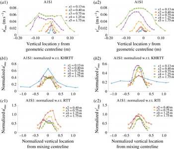
for A1S1 experiments.

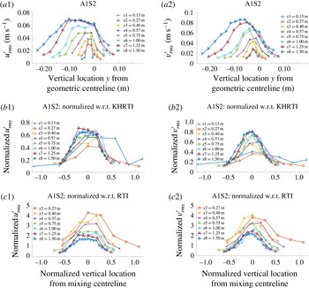
Actual and normalized velocity fluctuations (root-mean-square values)
 $u_{rms}^{\prime }$
and
 $v_{rms}^{\prime }$
for A1S2 experiments.

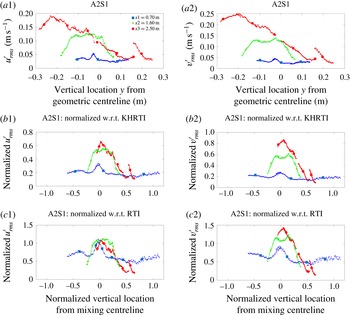
Actual and normalized velocity fluctuations (root-mean-square values)
 $u_{rms}^{\prime }$
and
 $v_{rms}^{\prime }$
for A2S1 experiments.

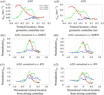
Actual and normalized velocity fluctuations (root-mean-square values)
 $u_{rms}^{\prime }$
and
 $v_{rms}^{\prime }$
for A2S2 experiments.

Actual and normalized velocity fluctuations (root-mean-square values)
 $u_{rms}^{\prime }$
and
 $v_{rms}^{\prime }$
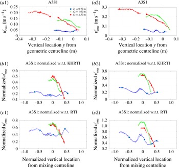
for A3S1 experiments.

3.2 Turbulence statistics
Velocity fluctuation measurements are made using hot-wire anemometry for A1 cases and PIV for all other cases. Density fluctuations are also measured for A1 cases using hot-wire anemometry and are used for calculating density–velocity fluctuation correlations (
 $\overline{\unicode[STIX]{x1D70C}^{\prime }v^{\prime }}$
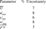
). Estimated uncertainties in hot-wire measurements (Kraft Reference Kraft2008) have been summarized in table 4. Details about
 $\unicode[STIX]{x1D70C}^{\prime }$
measurements and molecular mixing are presented in Akula et al. (Reference Akula, Andrews and Ranjan2013). Mean streamwise velocity profiles
 $\overline{U}(y)$
for A1 cases are shown in figure 9. General trends observed here (such as shifting of profiles below the geometric centreline and their spreading when approaching the low-speed stream velocity) have been discussed previously in § 3.1.4. Slopes of these curves and their interpolated values were used to obtain velocity gradients for Richardson number calculations in § 3.1.3.
Estimated uncertainties in hot-wire measurements.

3.2.1 Velocity fluctuations
Profiles of velocity fluctuations (root-mean-square values) in streamwise (
 $u_{rms}^{\prime }=\sqrt{\overline{{u^{\prime }}^{2}}}$
) and cross-stream (
 $v_{rms}^{\prime }=\sqrt{\overline{{v^{\prime }}^{2}}}$
) directions across the mixing layer are shown in panels (a1) and (a2) of figures 10–14. The
 $v_{rms}^{\prime }$
profiles for A1 cases look Gaussian-like. The
 $u_{rms}^{\prime }$
profiles for A1 cases show a flatter distribution, specifically after the first few
 $x$
locations. Profiles at location
 $x3$
for cases A2S1 and A2S2, and profiles at both locations
 $x2$
and
 $x3$
for case A3S1 are incomplete. Also, discrepancies in stitching between PIV cameras at location
 $x2$
for cases A2S1 and A2S2 make interpretation difficult. However, the overall trends look similar to A1 cases. The
 $v_{rms}^{\prime }$
profiles appear Gaussian-like and the
 $u_{rms}^{\prime }$
profiles show flatter shapes.
An attempt has been made to scale these velocity fluctuations using a combination of KHI and RTI scaling techniques. We assume that
 $v^{\prime }$
can be scaled by the derivative of the mixing width with respect to time,
 ${\dot{h}}$
. Applying this same concept to (3.2), we find
 $$\begin{eqnarray}v_{khrt}^{\prime }\sim {\dot{h}}\sim C_{1}\unicode[STIX]{x0394}U+C_{2}A_{t}g\left(\frac{x}{U}\right).\end{eqnarray}$$
Values of
 $C_{1}$
and
 $C_{2}$
can be chosen based on the relative strength of shear and buoyancy in the regime of interest of the flow. To determine a single velocity scale,
 $C_{1}$
is taken to be equal to
 $\unicode[STIX]{x1D6FD}$
and
 $C_{2}=2\unicode[STIX]{x1D6FC}$
, where
 $\unicode[STIX]{x1D6FD}$
and
 $\unicode[STIX]{x1D6FC}$
are growth rate parameters from table 2. This scaling is referred to as scaling with respect to KHRT or KHRTI scaling (
 $v_{khrt}^{\prime }$
). Choosing
 $C_{1}=0$
or
 $C_{2}=0$
is referred to as scaling with respect to RTI (
 $v_{rt}^{\prime }$
) or KHI (
 $v_{kh}^{\prime }$
), respectively. The vertical location
 $y$
is normalized similar to Pope (Reference Pope2000) as
 $y_{norm}=(y-y_{0}(x))/h(x)$
, where
 $h(x)$
is the mixing width (3.2) at location
 $x$
and
 $y_{0}$
is the vertical location where
 $\overline{U}(y)\approx (U_{1}+U_{2})/2$
. Normalized profiles of
 $u_{rms}^{\prime }$
and
 $v_{rms}^{\prime }$
for KHRT cases are shown in panels (b) and (c) of figures 10–14. In all these figures, panel (b) shows normalization with respect to the KHRTI scale and panel (c) shows normalization with respect to the RTI scale. Normalization using only the KHI scale (
 $C_{2}=0$
) does not give any coherent scaling and thus is ignored.
For A1 cases,
 $v_{khrt}^{\prime }$
normalizes
 $u_{rms}^{\prime }$
better than
 $v_{rt}^{\prime }$
. Scaling is the best for A1S1, where only the profile at
 $x1$
deviates from a collapse. At the early location
 $x1$
, the flow is shear dominated. Similarly, the profiles of case A1S2 at initial
 $x$
locations do not follow the scaling. The larger shear and delayed transition from shear to buoyancy in case A1S2 could explain why the deviation from the scale persists for longer time. Scaling of
 $v_{rms}^{\prime }$
is not as good as
 $u_{rms}^{\prime }$
when using
 $v_{khrt}^{\prime }$
. This trend is observed in general for A2–A3 cases as well.
 $v_{rms}^{\prime }$
scales better with
 $v_{rt}^{\prime }$
for most of the A1–A3 cases (this is when
 $x1$
is not considered for A1 cases;
 $x1$
data dropped from the bottom of panel (c) of figures 10 and 11). For A3S1,
 $v_{rms}^{\prime }$
profiles at
 $x2$
and
 $x3$
scale better with
 $v_{khrt}^{\prime }$
. Buoyancy plays the dominant role in affecting cross-stream velocity fluctuations and thus these velocity components scale better when normalized by
 $v_{rt}^{\prime }$
at late times. Another irregular trend is that RTI scaling is better even for
 $u_{rms}^{\prime }$
for A2S1 and A3S1 cases, while
 $v_{khrt}^{\prime }$
scales
 $u_{rms}^{\prime }$
better for A2S2. When comparing between cases, the scaling on vertical axes generally looks much more consistent when KHRT normalization is used rather than RTI normalization.
To summarize, the proposed scaling with
 $v_{khrt}^{\prime }$
is adequate for intermediate stages of the flow when transition from shear to buoyancy dominance is taking place. A single velocity scale may not be relevant throughout the flow. The shear and buoyancy-dominated stages of the flow scale appropriately with KH and RT scales, respectively. One expected yet important observation is that the chosen scaling for the vertical location
 $y$
performs well, suggesting that the points of maximum
 $u_{rms}^{\prime }$
and
 $v_{rms}^{\prime }$
roughly coincide with the vertical location where
 $\overline{U}(y)\approx (U_{1}+U_{2})/2$
. This location in the mixing width is used when calculating probability density functions and energy spectra.
3.2.2 Probability density functions
The probability density function (p.d.f.) of a continuous random variable describes the likelihood of the variable to have a particular value (Papoulis & Pillai Reference Papoulis and Pillai2002; Bendat & Piersol Reference Bendat and Piersol2010; Davidson Reference Davidson2015). Mathematically, the definite integral of p.d.f.
 $p(x)\,\text{d}x$
from
 $x_{1}$
to
 $x_{2}$
gives the probability of variable
 $x$
taking values between
 $x_{1}$
and
 $x_{2}$
. This implies that
 $\int _{-\infty }^{+\infty }p(x)\,\text{d}x=1$
. In the present context, the p.d.f. of a variable, say streamwise velocity fluctuation
 $u^{\prime }$
, indicates the relative amount of fluid whose velocity fluctuation is that value of
 $u^{\prime }$
. Here, the p.d.f. is calculated for quantities varying in time at a particular spatial location, which is approximately the point of maximum
 $u_{rms}^{\prime }$
or
 $v_{rms}^{\prime }$
(discussed previously in § 3.2.1). Apart from the p.d.f., two more statistical quantities, skewness and kurtosis, are reported (Wygnanski & Fiedler Reference Wygnanski and Fiedler1970; Champagne, Pao & Wygnanski Reference Champagne, Pao and Wygnanski1976; Groeneveld & Meeden Reference Groeneveld and Meeden1984; Joanes & Gill Reference Joanes and Gill1998). For fluctuating variable
 $u^{\prime }$
, an estimate of the skewness is
 $S_{u^{\prime }}=\overline{{u^{\prime }}^{3}}/\unicode[STIX]{x1D70E}_{u^{\prime }}^{3}$
and the kurtosis is
 $K_{u^{\prime }}=\overline{{u^{\prime }}^{4}}/\unicode[STIX]{x1D70E}_{u^{\prime }}^{4}$
, where
 $\unicode[STIX]{x1D70E}_{u^{\prime }}$
is the standard deviation of
 $u^{\prime }$
. For unimodal distributions, negative skewness indicates longer or fatter left tail in the p.d.f., and positive skewness indicates longer or fatter right tail. Skewness is zero for symmetric distributions such as the normal distribution. Kurtosis measures the degree of peakedness of a distribution. Sharp peaks in the p.d.f. produce larger kurtosis while a broader plateau-like p.d.f. produces a smaller kurtosis. The kurtosis of the normal distribution is 3. While these interpretations of skewness and kurtosis are useful, they can also be inconsistent, especially for multi-mode distributions.
The non-dimensional time
 $\unicode[STIX]{x1D70F}$
for KHRT cases is defined as
 $\unicode[STIX]{x1D70F}=(x/U)\sqrt{A_{t}g/H}$
, where
 $H$
is the effective tunnel height (1.2 m for the two-layer tunnel and 1.22 m for the multi-layer tunnel). In most numerical studies of RTI,
 $H$
is defined as the dominant wavelength of the initial perturbation (Cabot & Cook Reference Cabot and Cook2006). In the present experimental set-up, the p.d.f.s and energy spectra in § 3.2.3 are calculated for fluctuating quantities varying with time at a particular spatial location, and this corresponds to the variation along the mixing line for conventional box-type, transient experiments.
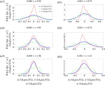
P.d.f.s of velocity fluctuations at different non-dimensional times
 $\unicode[STIX]{x1D70F}$
for A1S0 and A1S1 cases.

Panels (a) of figure 15 show the p.d.f.s of fluctuating velocity components
 $u^{\prime }$
,
 $v^{\prime }$
and
 $w^{\prime }$
(
 $w^{\prime }$
is the spanwise component) at
 $\unicode[STIX]{x1D70F}=0.53,1.03$
and 1.56 for case A1S0; velocities are normalized using the RTI scale
 $A_{t}g(x/U)$
. During the initial stage at
 $\unicode[STIX]{x1D70F}=0.53$
when the flow is not necessarily self-similar, p.d.f.s of
 $u^{\prime }$
and
 $v^{\prime }$
have broad distributions, indicating that the normalized root-mean-square of velocity fluctuations are higher than the corresponding self-similar values. This is in accordance with the higher values of RTI growth rate parameters
 $\unicode[STIX]{x1D6FC}_{b,s}$
observed at early stages of the instability (Akula et al.
Reference Akula, Andrews and Ranjan2013). Also, it can be seen that the p.d.f. of
 $w^{\prime }$
has a very large peak around zero, confirming the nearly two-dimensional nature of the flow at early times. The p.d.f.s of
 $u^{\prime }$
and
 $v^{\prime }$
are similar at
 $\unicode[STIX]{x1D70F}=0.53$
. Around this time,
 $v_{rms}^{\prime }/u_{rms}^{\prime }\approx 1$
. By the time
 $\unicode[STIX]{x1D70F}=1.03$
, the p.d.f. of spanwise component
 $w^{\prime }$
becomes similar to the distribution for
 $u^{\prime }$
, indicating transition into three-dimensional flow. The ratio
 $v_{rms}^{\prime }/u_{rms}^{\prime }$
becomes greater than 1.5 at late times (Akula & Ranjan Reference Akula and Ranjan2016). The broader p.d.f. of
 $v^{\prime }$
at late times is a characteristic for RTI flows (Banerjee, Kraft & Andrews Reference Banerjee, Kraft and Andrews2010b
; Akula & Ranjan Reference Akula and Ranjan2016), due to the broad spectrum of scales that develop from rising bubbles and falling spikes. It also indicates that large fluid blobs exhibit these random vertical motions.
Panels (b) of figure 15 show the p.d.f.s of fluctuating velocity components
 $u^{\prime }$
,
 $v^{\prime }$
and
 $w^{\prime }$
at
 $\unicode[STIX]{x1D70F}=0.37,0.74$
and 1.12 for KHRT case A1S1. The
 $u^{\prime }$
profile looks Gaussian-like at all times, similar to RTI flows. The widths of these Gaussian-like profiles are different at each time, due to the scaling of the velocity fluctuation. At an early time
 $\unicode[STIX]{x1D70F}=0.37$
, when the flow is KHI dominated, the velocity fluctuation does not scale with
 $A_{t}g(x/U)$
and the p.d.f. shape is much broader. Although the flow is primarily two-dimensional at this time, the p.d.f. of
 $w^{\prime }$
looks broader due to the improper choice of scaling. The ratio
 $v_{rms}^{\prime }/u_{rms}^{\prime }$
at this time is less than 1, which is a characteristic of KHI mixing layers (Bell & Mehta Reference Bell and Mehta1990; Pope Reference Pope2000). The location at
 $\unicode[STIX]{x1D70F}=0.74$
falls in the KH to RT transition region, and the mixing layer is three-dimensional by this point. The p.d.f. of
 $u^{\prime }$
is Gaussian-like and mostly symmetric about the zero mean. The ratio
 $v_{rms}^{\prime }/u_{rms}^{\prime }$
exceeds 1 at this location, as the mixing layer begins to show characteristics of RTI. At
 $\unicode[STIX]{x1D70F}=1.12$
, the flow becomes RTI dominated and all the p.d.f.s show characteristics similar to the self-similar RTI mixing layer of case A1S0 at
 $\unicode[STIX]{x1D70F}=1.56$
(comparing panels (a2), (a3) and (b3) of figure 15).
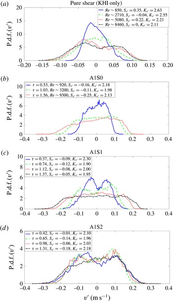
P.d.f.s of vertical (cross-stream) velocity fluctuations
 $v^{\prime }$
at different non-dimensional times
 $\unicode[STIX]{x1D70F}$
for a pure shear case (a) and A1 cases (b–d), along with skewness and kurtosis values.

P.d.f.s of vertical velocity fluctuations (without normalization) are given special attention due to their interesting behaviour. Figure 16 shows p.d.f.s of
 $v^{\prime }$
at different non-dimensional times for a pure shear case and A1 cases. Skewness and kurtosis values are also reported. For the shear case, a suitable Reynolds number is defined as
 $Re=h\unicode[STIX]{x0394}U/\unicode[STIX]{x1D708}$
, where
 $h$
is the total mixing width and
 $\unicode[STIX]{x1D708}$
is the coefficient of kinematic viscosity (Akula Reference Akula2014). For RT and KHRT cases, a suitable Reynolds number is defined (Akula et al.
Reference Akula, Andrews and Ranjan2013; Akula Reference Akula2014; Akula & Ranjan Reference Akula and Ranjan2016) as
 $Re=(h^{3/2}/\unicode[STIX]{x1D708}_{mix})\sqrt{gA_{t}/6}$
, where
 $\unicode[STIX]{x1D708}_{mix}$
is obtained as per Wilke (Reference Wilke1950). These Reynolds numbers are included in the p.d.f. and energy spectra figures wherever appropriate. For the pure shear case (panel (a) of figure 16), the p.d.f. of
 $v^{\prime }$
is Gaussian-like at small Reynolds numbers (at early times). As the Reynolds number increases, the kurtosis decreases, indicating that the p.d.f. is deviating from Gaussian. The skewness values are small, indicating symmetry as fluctuations from both top and bottom streams are being entrained into the centre of the mixing layer. The p.d.f. shape also becomes double peaked as roll-up structures develop at higher Reynolds numbers. The double peaked p.d.f. of
 $v^{\prime }$
could be a characteristic of KHI flows with well-developed large coherent roll-ups, as explained later qualitatively. For RTI flows (panel (b) of figure 16), the p.d.f.s of
 $v^{\prime }$
at different times show flatter distributions indicating an equal contribution from a broad spectrum of scales (Banerjee et al.
Reference Banerjee, Kraft and Andrews2010b
; Akula & Ranjan Reference Akula and Ranjan2016). The skewness is close to zero, suggesting symmetry. The kurtosis is
 ${\approx}2$
, due to the flatness of the p.d.f. shapes. For the KHI case, although the shapes of the p.d.f.s are different compared to the RTI case, the kurtosis values are still
 ${\approx}2$
at high Reynolds numbers. For A1S1 and A1S2 cases, the p.d.f.s of
 $v^{\prime }$
are shown in panels (c) and (d) of figure 16. The p.d.f.s show double peaked distributions at early times and flat RTI-like distributions at later times. This change in p.d.f.s could be used to predict KH to RT transition, but is not investigated in the present paper. The flattening of the distribution can be interpreted as an increase in the number of peaks with time, indicating generation of structures of varying size due to nonlinear interactions. The p.d.f. shapes eventually look similar to the ones seen in RTI-dominated flows at late times for both A1S1 and A1S2 cases. The kurtosis remains roughly constant throughout the p.d.f. evolution at
 ${\approx}2$
. The skewness is always negative, but very close to zero at all times. Negative skewness indicates that the largest fluctuations are seen in the downward direction.
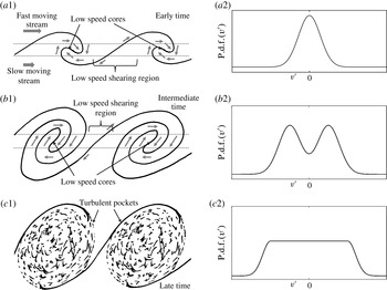
Schematics in (a1,b1,c1) to show development of KHI roll-ups and their subsequent stretching, and how they contribute to multiple peaks in p.d.f.s of velocity fluctuations. In (a2,b2,c2), representative p.d.f. distributions are shown.

Panels (a1) and (b1) of figure 17 qualitatively explain the origin of double peaks (or multiple peaks, in general) in p.d.f.s of planar velocity fluctuations (
 $u^{\prime }$
and
 $v^{\prime }$
) at early stages of KHI flows or KHRT flows when shear is dominant. At early times when KHI roll-ups are developing, only a small amount of fluid in the vortex core exhibits rotational motion (marked as low-speed cores in panel (a1); arrows are used to show fluid motion). A large amount of stagnant fluid (only convected by the mean flow) is present near the interface of two fluids (marked as low-speed shearing region in panel (a1)). Now, if a p.d.f. of
 $v^{\prime }$
is calculated at the centre of the mixing layer, its shape is likely to be Gaussian-like, centred at zero and having small standard deviation (panel (a2)) as most of the fluid is still stagnant. At intermediate stages of the flow (panel (b1)), roll-ups become well developed and have a coherent structure. More fluid is now showing rotational motion around the low-speed vortex cores and only a small amount of stagnant fluid is present in the shearing region. In other words, more fluid has a positive or negative velocity, and less fluid is stagnant. This gives rise to the double peaked p.d.f. of
 $v^{\prime }$
, shown in panel (b2). Depending upon how misaligned the measurement point is from the actual mixing centre and the orientation of the velocity vectors (as shown in panels (a1) and (b1)), the p.d.f. can be skewed, can have multiple (two or more) peaks, or the p.d.f. of
 $u^{\prime }$
can exhibit multiple peaks. At late stages when shear roll-ups are no longer coherent (due to merging with large turbulent roll-ups or stretching due to RTI), we find turbulent pockets as shown in panel (c1). A wide range of velocity scales develop and the p.d.f. looks flat as shown in panel (c2). Note that the representative p.d.f.s shown in the right column in figure 17 are idealized. For example, as was observed from the top panel (a) of figure 16, double peaks in the p.d.f. of
 $v^{\prime }$
can persist till late times.
P.d.f.s of vertical turbulent mass flux
 $\unicode[STIX]{x1D70C}^{\prime }v^{\prime }$
at different streamwise locations and corresponding non-dimensional times
 $\unicode[STIX]{x1D70F}$
for A1 cases, along with skewness and kurtosis values.

The vertical turbulent mass flux
 $\unicode[STIX]{x1D70C}^{\prime }v^{\prime }$
is an important quantity for turbulence transport in RTI and KHRT flows (Mueschke & Schilling Reference Mueschke and Schilling2009a
,Reference Mueschke and Schilling
b
; Banerjee et al.
Reference Banerjee, Kraft and Andrews2010b
; Akula & Ranjan Reference Akula and Ranjan2016). Figure 18 shows p.d.f.s of
 $\unicode[STIX]{x1D70C}^{\prime }v^{\prime }$
(normalized with RT scale
 $\unicode[STIX]{x0394}\unicode[STIX]{x1D70C}A_{t}g(x/U)$
) for all three A1 cases at different streamwise locations and corresponding non-dimensional times, along with skewness and kurtosis values. Late time p.d.f.s scale quite well with the chosen RT scale, as expected. Large and sharp peaks are found around 0 for most of the cases, resulting in large kurtosis values. P.d.f.s have longer and fatter tails on the left (negative skewness). This is a characteristic of RT-dominated flows (Banerjee et al.
Reference Banerjee, Kraft and Andrews2010b
; Akula & Ranjan Reference Akula and Ranjan2016) where
 $\unicode[STIX]{x1D70C}^{\prime }$
and
 $v^{\prime }$
are strongly negatively correlated, and it indicates predominantly rising motion of lighter fluid particles and falling motion of heavier fluid particles. An exception to this trend is the first
 $x$
location for A1S0 and A1S1 where there is greater probability of positive
 $\unicode[STIX]{x1D70C}^{\prime }v^{\prime }$
. The cross-correlation coefficient
 $R_{\unicode[STIX]{x1D70C}^{\prime }v^{\prime }}=\overline{\unicode[STIX]{x1D70C}^{\prime }v^{\prime }}/(\unicode[STIX]{x1D70C}_{rms}^{\prime }v_{rms}^{\prime })$
values for all three A1 cases are shown in table 5 at different streamwise locations. The value of
 $R_{\unicode[STIX]{x1D70C}^{\prime }v^{\prime }}\sim -0.8$
for A1S0 is close to the earlier reported values in Cook & Dimotakis (Reference Cook and Dimotakis2001), Ristorcelli & Clark (Reference Ristorcelli and Clark2004), Kraft (Reference Kraft2008), Akula & Ranjan (Reference Akula and Ranjan2016), and this value indicates a strong negative correlation between
 $\unicode[STIX]{x1D70C}^{\prime }$
and
 $v^{\prime }$
as explained previously. Magnitudes of
 $R_{\unicode[STIX]{x1D70C}^{\prime }v^{\prime }}$
for A1S1 case are relatively smaller than those of pure RTI case A1S0 due to the presence of shear. Magnitudes of
 $R_{\unicode[STIX]{x1D70C}^{\prime }v^{\prime }}$
are even smaller for A1S2 case due to the presence of larger shear.
Cross-correlation coefficient
 $R_{\unicode[STIX]{x1D70C}^{\prime }v^{\prime }}=\overline{\unicode[STIX]{x1D70C}^{\prime }v^{\prime }}/(\unicode[STIX]{x1D70C}_{rms}^{\prime }v_{rms}^{\prime })$
at different streamwise locations for A1 cases.

3.2.3 Energy spectra
Energy spectra (Tennekes & Lumley Reference Tennekes and Lumley1972; Pope Reference Pope2000; Davidson Reference Davidson2015) obtained due to contribution of different fluctuating quantities provide useful insight into the development of turbulent length scales. Spectra for three components of velocity fluctuations (
 $u^{\prime }$
,
 $v^{\prime }$
and
 $w^{\prime }$
), density fluctuation
 $\unicode[STIX]{x1D70C}^{\prime }$
and vertical turbulent mass flux
 $\unicode[STIX]{x1D70C}^{\prime }v^{\prime }$
are presented for all A1 cases and a pure shear experiment, using hot-wire measurements. Although the measurements are made for frequency with the present convective-type set-up, they relate to wavenumbers along the mixing line for conventional, box-type set-ups. The frequency measurement becomes the wavenumber. This wavenumber is non-dimensionalized with the effective tunnel height
 $H$
. Discrete Fourier transforms, using the fast Fourier transform function of MATLAB®, are used to obtain the spectra (Pope Reference Pope2000)
 $$\begin{eqnarray}E_{\unicode[STIX]{x1D719}}(\unicode[STIX]{x1D705})=\left|\frac{1}{N}\mathop{\sum }_{n=1}^{N}\unicode[STIX]{x1D719}(n)\text{e}^{-\text{i}2\unicode[STIX]{x03C0}(\unicode[STIX]{x1D705}-1)(n-1)/N}\right|^{2},\end{eqnarray}$$
where
 $\unicode[STIX]{x1D719}=u^{\prime },v^{\prime },w^{\prime },\unicode[STIX]{x1D70C}^{\prime },\unicode[STIX]{x1D70C}^{\prime }v^{\prime }$
. The wavenumber is defined as
 $\unicode[STIX]{x1D705}=2\unicode[STIX]{x03C0}/\unicode[STIX]{x1D706}$
, where
 $\unicode[STIX]{x1D706}$
is the wavelength. The largest wavelength
 $L$
(corresponding to the smallest wavenumber
 $K$
) is defined as the product of the total sampling or measurement time
 $T$
and the average convective speed
 $U$
;
 $L=UT$
.
Compensated energy spectra for velocity fluctuations at different times, for A1 cases and a pure shear case.

Compensated spectra for density fluctuations at different times, for A1 cases.

Compensated spectra for vertical turbulent mass flux at different times, for A1 cases.

Spectra for
 $u^{\prime }$
,
 $v^{\prime }$
,
 $\unicode[STIX]{x1D70C}^{\prime }$
and
 $\unicode[STIX]{x1D70C}^{\prime }v^{\prime }$
at different streamwise locations and corresponding non-dimensional times, for A1S0 case.

Spectra for
 $u^{\prime }$
,
 $v^{\prime }$
,
 $\unicode[STIX]{x1D70C}^{\prime }$
and
 $\unicode[STIX]{x1D70C}^{\prime }v^{\prime }$
at different streamwise locations and corresponding non-dimensional times, for A1S1 case.

Spectra for
 $u^{\prime }$
,
 $v^{\prime }$
,
 $\unicode[STIX]{x1D70C}^{\prime }$
and
 $\unicode[STIX]{x1D70C}^{\prime }v^{\prime }$
at different streamwise locations and corresponding non-dimensional times, for A1S2 case.

Figure 19 shows the compensated spectra for all velocity fluctuations with
 $E$
normalized by KH. To check for Kolmogorov–Obukhov
 $\unicode[STIX]{x1D705}^{-5/3}$
law (Kolmogorov Reference Kolmogorov1941a
,Reference Kolmogorov
b
; Obukhov Reference Obukhov1941; Kolmogorov Reference Kolmogorov1962; Obukhov Reference Obukhov1962) in the inertial subrange (Tennekes & Lumley Reference Tennekes and Lumley1972; Pope Reference Pope2000; Davidson Reference Davidson2015), the energy on the vertical axis is also multiplied (compensated) with
 $(\unicode[STIX]{x1D705}H)^{5/3}$
, allowing the inertial subrange to appear as a horizontal line. The inertial subrange contains the scales for energy cascade (Tennekes & Lumley Reference Tennekes and Lumley1972; Pope Reference Pope2000; Davidson Reference Davidson2015). Panels (a1) and (a2) of figure 19 show velocity spectra at two streamwise locations for case A1S0. Panels (b1) and (b2) show spectra for a pure shear case. For A1S0 at
 $\unicode[STIX]{x1D70F}=0.54$
(panel (a1)), when the flow is still in early stages, neither the
 $v^{\prime }$
spectrum nor the
 $w^{\prime }$
spectrum show noticeable inertial subranges, but the spectrum for
 $u^{\prime }$
shows some inertial subrange (approximately a decade). The small scales have not yet developed at this time. At a later time
 $\unicode[STIX]{x1D70F}=1.52$
(panel (a2)), all three components show approximately one-and-a-half decades of inertial subrange. For the KHI case, at an early time (panel (b1)) when
 $Re\sim 4500$
, the flow is mostly dominated by large wavelengths, with no noticeable inertial subrange for any velocity component. At a later time (panel (b2)) when
 $Re\sim 9000$
, the mixing layer becomes three-dimensional and spectra show approximately one-and-a-half decades of
 $k^{-5/3}$
scaling for all velocity components. Panels (c) and (d) of figure 19 show the compensated spectra for velocity fluctuations for A1S1 and A1S2 cases, respectively. For these coupled instability cases, the spectra evolution is very similar to the RTI case. The spectra here for all three components start showing inertial subrange scaling even for early times (comparing panels (c1), (d1) with (a1), (b1)), indicating that the coupled instability cases transition to turbulence faster than purely KHI or RTI cases. Early transition for
 $u^{\prime }$
is observed again. Approximately one-and-a-half decades of inertial subrange are seen at late times.
Figure 20 shows the compensated spectra for density fluctuations for A1 cases. The density spectra have shown an inertial subrange from earlier times compared to velocity spectra. This observation is more apparent from figures 22–24. The spectra show approximately one to one-and-a-half decades of inertial subrange at late times. For their stratified wake simulation, de Stadler, Sarkar & Brucker (Reference de Stadler, Sarkar and Brucker2010) also observed the density field showing inertial subrange scales far earlier than the turbulent kinetic energy (Pope Reference Pope2000). This observation might provide further insight into why the density layer is thicker than the velocity layer, as discussed in § 3.1.4.
Figure 21 shows the compensated spectra for vertical turbulent mass flux for A1 cases. At early times, no inertial subrange is seen for any of the cases. At late times, the spectra show quite narrower inertial subrange compared to that of velocity and density fluctuations. This can again be seen from figures 22–24. The narrow inertial subrange for vertical turbulent mass flux may be attributed to difference in the extent and overlap of inertial subranges for vertical velocity and density fluctuations.
Spectra (without compensation) for
 $u^{\prime }$
,
 $v^{\prime }$
,
 $\unicode[STIX]{x1D70C}^{\prime }$
and
 $\unicode[STIX]{x1D70C}^{\prime }v^{\prime }$
for A1 cases at different streamwise locations and corresponding non-dimensional times are shown in figures 22–24. Fiducial slope lines corresponding to
 $\unicode[STIX]{x1D705}^{-5/3}$
are included in panels (c), (d) and (e). At early times of the instability growth, shown in panels (a) and (b) of each figure, no distinct structure appears in the spectra. However, moving from panel (a) to panel (e) in each figure, one notices features of turbulence onset, such as the development of an inertial subrange. In general, velocity and density exhibit similar scaling in the inertial subrange, but this scaling is steeper than
 $\unicode[STIX]{x1D705}^{-5/3}$
. This suggests that the exponent
 $p$
in the power-law spectrum
 $E(\unicode[STIX]{x1D705})\sim \unicode[STIX]{x1D705}^{-p}$
(Pope Reference Pope2000) is higher than
 $5/3$
for buoyancy affected flows. Previous estimates of such exponents for buoyancy affected flows include
 $p=7/4$
(Mikaelian Reference Mikaelian1989; Zhou Reference Zhou2001),
 $p=2$
(Poujade Reference Poujade2006; Abarzhi Reference Abarzhi2010; Sreenivasan & Abarzhi Reference Sreenivasan and Abarzhi2013) and
 $p=11/5$
(Bolgiano Reference Bolgiano1959; Obukhov Reference Obukhov1959; Lohse & Xia Reference Lohse and Xia2010; Zhou Reference Zhou2013; Kumar, Chatterjee & Verma Reference Kumar, Chatterjee and Verma2014; Zhou et al.
Reference Zhou, Huang, Lu, Liu and Ni2016; Boffetta & Mazzino Reference Boffetta and Mazzino2017). Despite sharing similar power-law scaling, the inertial subrange of the
 $\unicode[STIX]{x1D70C}^{\prime }$
spectra is longer than the velocity spectra, implying earlier exhibition of inertial subrange for density field. Strong correlation exits between the spectra for
 $v^{\prime }$
and
 $\unicode[STIX]{x1D70C}^{\prime }v^{\prime }$
, as was also observed for RTI flows by Banerjee et al. (Reference Banerjee, Kraft and Andrews2010b
). Spectra of
 $u^{\prime }$
show different power-law scaling in the inertial subrange depending on the amount of shear present. In the case with no shear, the spectra plot for
 $u^{\prime }$
closely matches that for
 $v^{\prime }$
. As the amount of shear increases, the
 $u^{\prime }$
spectra deviates from
 $v^{\prime }$
and begins to follow the
 $\unicode[STIX]{x1D705}^{-5/3}$
law, as apparent from the bottom panels of figure 24. This could be due to the
 $\unicode[STIX]{x1D705}^{-5/3}$
law for KHI-dominated flows (Townsend Reference Townsend1980; Werne & Fritts Reference Werne and Fritts1999), and prolonged shear dominance and late transition into the RTI regime for case A1S2.
Velocity spectra (without compensation) for
 $u^{\prime }$
and
 $v^{\prime }$
at different streamwise locations and corresponding non-dimensional times are shown in figures 25 and 26, for A2–A3 cases. PIV is used to obtain velocity fluctuations around maximum
 $u_{rms}^{\prime }$
or
 $v_{rms}^{\prime }$
for these cases as hot-wire measurements were made only at the geometric centreline. As PIV measurements are spaced by
 $1/15$
s in time and although this frequency along with the number of images collected represent statistically steady statistics of the flow (see the discussion on PIV in § 2.3), these measurements are inadequate for spectra calculations. Thus, measurements are made for wavenumbers along the mixing line (similar to conventional, box-type set-ups) by treating the PIV window as a box-type experiment. The largest wavenumbers obtained using this approach are of the same order of magnitude as those from hot-wire measurements for the A1 cases, as seen by comparing the right limits of the horizontal axes of figures 25 and 26 with those of earlier figures showing spectra. However, due to the small size of PIV windows, large wavelengths (small wavenumbers) are not properly captured, as seen by comparing the left limits of the horizontal axes of figures 25 and 26 with those of previous spectra. In figures 25 and 26, fiducial slope lines corresponding to
 $\unicode[STIX]{x1D705}^{-3}$
,
 $\unicode[STIX]{x1D705}^{-5/2}$
,
 $\unicode[STIX]{x1D705}^{-2}$
,
 $\unicode[STIX]{x1D705}^{-7/4}$
and
 $\unicode[STIX]{x1D705}^{-5/3}$
are also shown for comparison (see table 6). At late times, the velocity spectra show
 $\unicode[STIX]{x1D705}^{-p}$
dependence in the inertial subrange with
 $2\lesssim p\lesssim 5/2$
. This indicates that the measured/resolved small scales at present Reynolds number do not achieve three-dimensional isotropy, for A2–A3 cases with the discussed method of calculating spectra.
Some commonly used power-law energy spectra for velocity fluctuations in turbulent flows.

Energy spectra for
 $u^{\prime }$
and
 $v^{\prime }$
at different streamwise locations and corresponding non-dimensional times, for A2S0 and A2S1 cases.

4 Conclusions
This paper summarizes the essential dynamics of the coupled Rayleigh–Taylor (RT) and Kelvin–Helmholtz (KH) instability studied using statistically steady experiments performed in a multi-layer gas tunnel. Experiments are performed at four Atwood numbers ranging from 0.035 to 0.159, with varying amount of shear ranging
 $\unicode[STIX]{x0394}U/U$
from 0 to 0.48. Three types of diagnostics – back-lit visualization, hot-wire anemometry and particle image velocimetry – are employed to obtain the mixing widths, velocity field and density field.
Owing to linear self-similar temporal growth for KHI and quadratic growth for RTI, the flow is KHI dominated at early times and RTI dominated at late times. This transition from KHI-like to RTI-like behaviour is quantified using the Richardson number: the non-dimensional number used to quantify the relative strength of buoyancy to shear. The transitional Richardson number magnitudes obtained for the present KHRT flows, i.e. unstably stratified free shear flows, are in the range 0.17–0.56. This range closely resembles the critical Richardson number range for stably stratified free shear flows. For this latter category of flows, turbulence starts to decay after the critical Richardson number is reached. This similarity between unstably and stably stratified free shear flows could be of great importance for atmospheric and oceanic fluid mechanics. Also, the KH to RT transition criterion based on transitional Richardson number should be useful for numerical hydrodynamic solvers to decide between KHI and RTI related turbulence models.
A comparison of the evolution of density and velocity mixing widths is presented. The density mixing layer is observed to grow approximately two times as thick but symmetrically compared to the velocity mixing layer. This observation is consistent with some of the previous works (Dimotakis Reference Dimotakis1991), and can be attributed to enhanced mass transport arising from diffusion as well as fluid entrainment due to turbulent shear and buoyancy.
Scaling of velocity fluctuations is investigated using combinations of KH and RT scales. It is found that the proposed KHRT velocity scale, obtained using the combined mixing-layer growth equation (3.2), is appropriate for intermediate stages of the flow when both KH and RT dynamics are comparable. A single velocity scale may not be relevant throughout the flow. Probability density functions for different fluctuating quantities are presented. Multiple peaks in p.d.f.s are qualitatively explained from the development of coherent KH roll-ups and their subsequent transition into turbulent pockets. The evolution of energy spectra for the studied flows indicates that density fluctuations start to show an inertial subrange from earlier times compared to velocity fluctuations. The spectra exhibit slightly steeper slope than Kolmogorov–Obukhov five-thirds law in the inertial subrange. Previous studies do suggest such steeper slopes for buoyancy affected flows.
The data, analyses and discussions presented in this paper, originating from statistically steady experiments, are expected to be very useful for instability-driven turbulence research and related meteorological phenomena.
Energy spectra for
 $u^{\prime }$
and
 $v^{\prime }$
at different streamwise locations and corresponding non-dimensional times, for A2S2 and A3S1 cases.

Acknowledgement
This work was supported by the US DOE-NNSA SSAA grant no. DE-NA0002575.