

1 Introduction
Buoyancy-driven atmospheric boundary layers capped by strong stable layers can be understood as a large-scale manifestation of turbulent Rayleigh–Bénard (R–B) convection (Deardorff Reference Deardorff1970; Brown Reference Brown1980; Wyngaard Reference Wyngaard1992). The presence of water vapour and its associated phase changes plays a central role in the nature of the convection (Bretherton Reference Bretherton1987, Reference Bretherton1988; Stevens Reference Stevens2005; Pauluis et al. Reference Pauluis and Schumacher2010; Pauluis & Schumacher Reference Pauluis and Schumacher2011; Mellado, Puche & van Heerwaarden Reference Mellado, Puche and van Heerwaarden2017). The general problem of moist convection, fully coupled with surface fluxes, large-scale dynamics, radiative transfer and cloud formation remains a grand challenge, with relevance to weather forecasting and climate. In this work, we set as a more modest goal the investigation of how water vapour supersaturation behaves in traditional Rayleigh–Bénard convection.
1.1 Moist convection parameters
The cloud topped convective-boundary-layer is effectively a Rayleigh–Bénard system driven by buoyancy forcing, e.g. radiative forcing from cloud top (Lilly Reference Lilly1968; Moeng & Rotunno Reference Moeng and Rotunno1990; Stevens Reference Stevens2005; Mellado Reference Mellado2017). In this system, continuous plume eruption from both boundaries transports heat and moisture and produces the mixed layer (Emanuel Reference Emanuel1994). The cloud aspect of the problem depends on the presence of water vapour, making this a case of two-scalar Rayleigh–Bénard convection. Similar to a single-component convection, the equivalent Rayleigh number (or the moist Rayleigh number for moist convection) determines the marginal stability of the convective system. For moist convection, it can be approximated as (Chillà & Schumacher Reference Chillà and Schumacher2012; Niedermeier et al. Reference Niedermeier, Chang, Cantrell, Chandrakar, Ciochetto and Shaw2018)
 $$\begin{eqnarray}Ra_{moist}\approx \frac{g\unicode[STIX]{x0394}TH^{3}}{T_{0}\unicode[STIX]{x1D708}D_{t}}+\frac{g\unicode[STIX]{x1D716}\unicode[STIX]{x0394}q_{v}H^{3}}{\unicode[STIX]{x1D708}D_{t}}.\end{eqnarray}$$
Here,  $\unicode[STIX]{x0394}T$,
 $\unicode[STIX]{x0394}q_{v}$ and
 $H$ are the applied temperature difference, the difference in the water vapour mixing ratio and length scale of the system, respectively. Other constants
 $g$,
 $\unicode[STIX]{x1D708}$ and
 $T_{o}$ are the gravitational acceleration, the kinematic viscosity and the mean temperature (reference temperature). The parameter
 $\unicode[STIX]{x1D716}=M_{a}/M_{w}-1$, where
 $M_{a}$ and
 $M_{w}$ are the molecular masses of dry air and water, respectively. The above relation is obtained by taking a ratio of buoyancy (
 ${\sim}\unicode[STIX]{x1D70C}g(\unicode[STIX]{x0394}T/T_{0}+\unicode[STIX]{x1D716}\unicode[STIX]{x0394}q_{v})$) and viscous force (
 ${\sim}\unicode[STIX]{x1D708}\unicode[STIX]{x1D70C}w^{\ast }/H^{2}$) scales and assuming that the destruction of density perturbation is larger because of the thermal diffusion than the diffusion of the other scalar (i.e. using
 $w^{\ast }\sim D_{t}/H$ as a velocity scale in the viscous forcing). Additionally, the velocity scale (
 $w^{\ast }$) is obtained from the flux balance between advection (
 ${\sim}w^{\ast }\unicode[STIX]{x1D6FF}T/H$) and diffusion (
 ${\sim}D_{t}\unicode[STIX]{x1D6FF}T/H^{2}$) of scalar perturbation from the base state. The scaling is therefore only valid when the thermal gradient is the largest contributor to buoyancy or when both scalars have the same molecular diffusivities. In the contrasting case where the second scalar contributes significantly, the diffusivity of the dominant scalar should be used. In the moist convection case, the water vapour’s contribution to the buoyancy is smaller than the thermal contribution (at least for the temperature range considered here). In the subsequent definition of the Rayleigh number, the underlying assumption is that the thermal gradient is a larger contributor to the buoyancy perturbation than the gradient of the other scalar. However, the contribution of the other scalar to buoyancy is not ignored. Other relevant non-dimensional variables associated with the fluid properties are the relative diffusivities of water vapour and thermal field, the Schmidt number (
 $Sc=\unicode[STIX]{x1D708}/D_{v}$) and Prandtl number (
 $Pr=\unicode[STIX]{x1D708}/D_{t}$). These quantify the rate at which the molecular diffusion of scalars destroys the buoyancy forcing. A non-dimensional quantity related to the geometry of a system, the aspect ratio of a convection cell, also influences the flow to some extent.
There is a similarity between double-diffusive convection (Schmitt Reference Schmitt1994; Kelley et al. Reference Kelley, Fernando, Gargett, Tanny and Özsoy2003) and the current case of moist convection. In both cases, there are two scalars involved in the problem which are advecting and diffusing. However, in the traditional double-diffusive convection, scalars usually have opposite contributions to the buoyancy and/or have opposite diffusive fluxes. In the current case of moist convection, both scalars contribute to positive buoyancy and diffusing in the same direction; therefore, it is closer to traditional R–B convection. Indeed, the current case can be expressed as single component R–B convection driven by a difference in virtual temperature. The novel aspect considered here is to explicitly consider the diffusivity difference between the two scalars, as expressed through the Lewis number  $Le\equiv D_{t}/D_{v}$. The relevance of Lewis number and differential diffusivity is motivated by the water vapour supersaturation, described next.
1.2 Supersaturation from two scalar fields
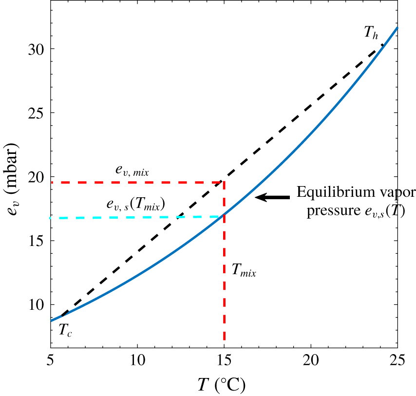
A thermodynamic vapour-pressure–temperature diagram illustrating the formation of supersaturation through isobaric mixing. An idealized mixing process of two saturated air parcels at different temperatures,  $T_{h}$ and
 $T_{c}$ (dashed line) and its comparison with the saturation (equilibrium) vapour pressure curve (blue line).

Supersaturation is central to cloud formation, whether it be in the earth’s atmosphere (Bohren & Albrecht Reference Bohren and Albrecht1998) or in the atmospheres of other planets and stars (Burrows et al. Reference Burrows, Marley, Hubbard, Lunine, Guillot, Saumon, Freedman, Sudarsky and Sharp1997; Marley et al. Reference Marley, Ackerman, Cuzzi and Kitzmann2013; Kreidberg et al. Reference Kreidberg, Bean, Désert, Benneke, Deming, Stevenson, Seager, Berta-Thompson, Seifahrt and Homeier2014). Taking water vapour as an example, supersaturation depends upon the two scalar fields’ temperature and water vapour mixing ratio through the water vapour pressure:  $s\equiv (e_{v}/e_{v,s}(T))-1$. Here,
 $e_{v}$ and
 $e_{v,s}$ are the water vapour pressure and saturation (or equilibrium) vapour pressure, respectively. The latter is expressed by the Clausius–Clapeyron equation,
 $e_{v,s}(T)\propto \exp (-{\mathcal{L}}/R_{v}T)$, where
 ${\mathcal{L}}$ is the latent heat of vaporization,
 $R_{v}$ is the mass-based gas constant for water vapour and
 $T$ is the temperature (Bohren & Albrecht Reference Bohren and Albrecht1998; Lamb & Shaw Reference Lamb and Shaw2016).
In turbulent R–B convection, scalar fields are advected and diffused, resulting in their mutual mixing. An idealized view of the mixing of two saturated air parcels is shown in figure 1, which depicts a thermodynamic space consisting of temperature and water vapour pressure. The equilibrium (Clausius–Clapeyron) curve is shown, and the mixing is assumed to take place between two air parcels with temperatures  $T_{h}$ and
 $T_{c}$ with a constant heat capacity. For isobaric mixing, various mass ratios result in the dashed line (Bohren & Albrecht Reference Bohren and Albrecht1998). The red dashed lines show a specific example of a fully mixed parcel with temperature
 $T_{mix}$ and water vapour pressure
 $e_{v,mix}$. It can be seen that
 $e_{v,mix}>e_{v,s}(T)$, resulting in a positive supersaturation in the mixture.
The idealization of figure 1 can be extended, taking into account the details of how temperature and water vapour fields are mixed in a turbulent flow. The relative humidity (RH  $\equiv e_{v}/e_{v,s}(T)$) problem has been the subject of considerable study in the boundary layer meteorology community, mainly focused on correlations between the two fields (e.g. Sorbjan Reference Sorbjan1989). The concept also underlies a common approach to representation of subgrid-scale variability of cloudiness. For example, Sommeria & Deardorff (Reference Sommeria and Deardorff1977) used the joint probability distribution function (p.d.f.) of two moist adiabatically conserved scalars to diagnose subgrid-scale cloud fraction, liquid water content and buoyancy flux in a large-eddy simulation of trade-wind cumulus clouds. Relative humidity variability is due to joint variability in the two conserved scalars and cloud is assumed to exist when relative humidity
 $RH\geqslant 1$. This approach has been extended by several others since then (e.g. Golaz, Larson & Cotton (Reference Golaz, Larson and Cotton2002a); Bogenschutz & Krueger (Reference Bogenschutz and Krueger2013) and references therein), in what have come to be known as p.d.f. methods. Further discussion of these approaches is in § 4.
1.3 An approach for studying scalar fields in moist Rayleigh–Bénard convection
This work is motivated by the problem of supersaturation in turbulent Rayleigh–Bénard convection within an idealized context, i.e. without the complications of large-scale shear, radiative transfer and condensate formation that exist in the atmosphere. The work’s origins are in questions that arose during the analysis and interpretation of observations taken in the ‘Pi chamber’, a laboratory chamber for studying cloud formation in turbulent R–B convection (Niedermeier et al. Reference Niedermeier, Chang, Cantrell, Chandrakar, Ciochetto and Shaw2018). In particular, the competing and complementary roles of diffusion versus advection are of interest, as is the relevance of differences in diffusivities for heat and for water vapour. For example, the seemingly negligible difference in diffusivities (Lewis number  $Le\equiv D_{t}/D_{v}=0.84$ at
 $20\,^{\circ }\text{C}$) has been used in other laboratory contexts as the underlying mechanism for precise control of supersaturation (Stratmann et al. Reference Stratmann, Kiselev, Wurzler, Wendisch, Heintzenberg, Charlson, Diehl, Wex and Schmidt2004).
We approach the problem of supersaturation in R–B convection using an idealized, one-dimensional model that faithfully represents the processes of advection and diffusion in turbulent flow. Using this kind of model allows a wide range of parameter space (e.g.  $Ra$) to be explored with computational efficiency and it is well suited to problems that are fundamentally dependent on advection and diffusion of scalars. It represents all relevant scales, so it captures the diffusive boundary layer as well as the larger-scale turbulent mixing in the bulk fluid. We consider this as a first exploration of the phenomenon at work, and more detailed approaches, such as using direct numerical simulation, will follow. Finally, the one-dimensional model is highly scalable, so it can be run at scales comparable to laboratory experiments with turbulent moist convection (Niedermeier et al. Reference Niedermeier, Chang, Cantrell, Chandrakar, Ciochetto and Shaw2018) and then can be scaled up for moist convection in the atmospheric boundary layer. The purpose here is to investigate the mean and fluctuating properties of the supersaturation field in turbulent moist Rayleigh–Bénard convection, in a general sense. Detailed comparison to laboratory experiments and exploration of the atmospheric context are challenges for future work.
The paper is organized as follows: in § 2 the One-Dimensional Turbulence (ODT) model is described and the parameters used in this study are defined. We then proceed to use the model to explore the scaling of heat and water vapour fluxes with relevant dimensionless variables (§ 3.1), fluctuations of scalars in the bulk fluid (§ 3.2), fluctuations of supersaturation in the bulk fluid (§ 3.4), vertical profiles of supersaturation in the boundary layer and the bulk fluid (§ 3.5) and the sampling within the thermodynamic space of water vapour pressure versus temperature (§ 3.3). Finally, we conclude the paper by summarizing and discussing the results in § 4.
2 Model description and problem set-up
The One-Dimensional Turbulence model was developed to simulate turbulent flows which are statistically homogeneous and isotropic in two dimensions but varying in the third (Kerstein Reference Kerstein1999). The ODT evolved from the linear eddy model (Kerstein Reference Kerstein1999), which has been previously used to simulate cloud turbulence (Krueger Reference Krueger1993; Krueger, Su & McMurtry Reference Krueger, Su and McMurtry1997). The ODT has been widely used for turbulence problems ranging from combustion (Echekki et al. Reference Echekki, Kerstein, Dreeben and Chen2001) to large-eddy simulation (LES) subgrid-scale modelling (Stechmann Reference Stechmann2014). Subsequent ODT development led to a version of the model specifically designed for problems involving buoyancy, either stably stratified (Wunsch & Kerstein Reference Wunsch and Kerstein2001) or convective (Wunsch & Kerstein Reference Wunsch and Kerstein2005; Gonzalez-Juez, Kerstein & Lignell Reference Gonzalez-Juez, Kerstein and Lignell2011). All versions of the ODT rely on the same basic construct. The flow is simulated on a line which is oriented along the direction in which mean flow properties vary, so for buoyant convection ODT represents the vertical coordinate. All fluid properties are functions of location along the line. Turbulent advection occurs through a series of random mappings of the ODT line onto itself. Mappings occur on all relevant length scales, and their statistics reproduce standard scaling relations for turbulence. During the intervals between mapping events, molecular diffusion is modelled using standard partial differential equations. The ODT results are typically interpreted statistically, e.g. by computing the mean and variance of each flow variable at each position along the line. Due to the restriction to one spatial dimension, it is computationally feasible to fully resolve the Kolmogorov scale. In the following paragraphs we provide an overview of the ODT model and readers are referred to the ODT references for details (Kerstein Reference Kerstein1999; Wunsch & Kerstein Reference Wunsch and Kerstein2001, Reference Wunsch and Kerstein2005).
To simulate moist convection using ODT, a variant of the version employed in Wunsch & Kerstein (Reference Wunsch and Kerstein2001, Reference Wunsch and Kerstein2005) is employed here. The ODT line is oriented along the  $z$ (vertical) axis. The flow variables are the magnitude of the velocity vector (
 $w$), temperature (
 $T$) and water vapour mixing ratio
 $q_{v}$. During the intervals between mappings, each of these variables (
 $X$) obeys
 $$\begin{eqnarray}(\unicode[STIX]{x2202}_{t}-D_{X}\unicode[STIX]{x2202}_{z}^{2})X=0.\end{eqnarray}$$
The boundary condition for the current problem is no-slip for velocity and water-vapour-saturated bottom and top boundaries at a fixed temperature (hot bottom and colder top). Note that the advection terms are absent from (2.1), and that the velocity variable ( $w$) does not actually move the fluid elements; in ODT the random mappings do that instead. Here
 $D_{X}$ represents molecular diffusivity of variable
 $X$. These equations are solved at full resolution (including all scales down to the viscous and/or diffusive scales). Full resolution of all length and time scales in turbulent flow is one of the key advantages of ODT simulations, and it is made computationally affordable by the restriction to one dimension. The fluid density variations are related to temperature and water vapour content by
 $$\begin{eqnarray}\unicode[STIX]{x1D70C}(q_{v},T)=\unicode[STIX]{x1D70C}_{o}\frac{T_{o}(1+\unicode[STIX]{x1D716}q_{v_{o}})}{T(1+\unicode[STIX]{x1D716}q_{v})},\end{eqnarray}$$
where  $\unicode[STIX]{x1D70C}_{o}$ and
 $q_{v_{o}}$ are the reference density and water vapour mixing ratio.
To simulate moist convection in the laboratory ‘Pi chamber’ with the ODT model, the velocity boundary conditions replicate no-slip walls at  $z=0$ and
 $z=H$ and fixed boundary condition for temperature and water vapour are applied. A temperature difference,
 $\unicode[STIX]{x0394}T$ is imposed across the convective cell and boundaries are assumed to be saturated with water at the temperature of each boundary. Therefore, there is also an imposed difference for water vapour (
 $\unicode[STIX]{x0394}q_{v}$) across the convective cell.
The physics of turbulent mixing is implemented in ODT through randomly selected mappings ( $M(z)$) of the line onto itself. The mapping is applied to all scalar fields simultaneously. It mimics the motion of a ‘fluid element’ and preserves the properties of each fluid element. The attributes of the mapping function have a strong impact on the model dynamics, so selection of an appropriate function is essential to constructing a realistic representation of turbulent advection within the one-dimensional framework. The mapping used in ODT is measure preserving. This is the one-dimensional equivalent of incompressibility, and implies that all statistical moments of scalar fields are preserved by the mapping. The mapping is also a continuous function, to avoid introducing discontinuities in mapped scalar fields. Finally, the function maps a finite region, to mimic a turbulent ‘eddy’ of defined length. The specific function
 $M(z)$ used here was introduced by Kerstein (Reference Kerstein1999) and is common to all versions of the ODT model (Wunsch & Kerstein Reference Wunsch and Kerstein2001),
 $$\begin{eqnarray}M(z)\equiv z_{o}+\left\{\begin{array}{@{}ll@{}}3(z-z_{o}),\quad & \text{if }z_{0}\leqslant z\leqslant z_{o}+L/3,\\ 2L-3(z-z_{o}),\quad & \text{if }z_{o}+L/3\leqslant z\leqslant z_{o}+2L/3,\\ 3(z-z_{o})-2L,\quad & \text{if }z_{o}+2L/3\leqslant z\leqslant z_{o}+L,\\ z-z_{o}\quad & \text{else,}\end{array}\right.\end{eqnarray}$$
where  $z_{o}$ is the location of the mapping event on a segment of length L. Essentially, this function takes the portion of the original scalar profile
 $T(z)$ between
 $z_{o}$ and
 $z_{o}+L$, compresses it to
 $1/3$ of its original size, and places three copies of this compressed profile within the original domain. The middle copy is reversed in order to maintain continuity. This mapping function has two additional attributes which are valuable for representing turbulent flows. The compression i.e. mixing of scalar profiles leads to a cascade of turbulent kinetic energy or scalar variance from large to small scales, as illustrated in Kerstein (Reference Kerstein1999) and Wunsch & Kerstein (Reference Wunsch and Kerstein2001). Also, the mapping results in a net scalar transport along the line when applied to a scalar field with a mean gradient. In the present context, this means that mappings will transport heat and water vapour vertically through the laboratory convection cell.
Since mappings do not change any statistical moment of a scalar field, they conserve kinetic energy. However, if vertical transport of scalars  $T$ or
 $q_{v}$ results in a change in potential energy, then energy conservation requires potential energy changes to be offset by corresponding changes in kinetic energy (conversion of potential to kinetic energy). The change in kinetic energy requires an additional operation on the velocity scalar, in addition to the applied mapping. The complete set of mapping and energy conserving operations applied to each scalar during a mapping event are given by
 $$\begin{eqnarray}\displaystyle & \displaystyle X(z)\rightarrow X(M(z)), & \displaystyle\end{eqnarray}$$
 $$\begin{eqnarray}\displaystyle & \displaystyle w(z)\rightarrow w(M(z))+c_{w}(z-M(z)), & \displaystyle\end{eqnarray}$$
 $(z-M(z))$ is the function added to the velocity scalar as part of the mapping process,
 $X$ represents scalars
 $T$ and
 $q_{v}$, and
 $c_{w}$ is a amplitude selected to enforce energy conservation. Energy conservation determines the constant
 $c_{w}$,
 $$\begin{eqnarray}c_{w}=\frac{27}{4L}\left[-w_{k}\pm \sqrt[]{w_{k}^{2}-\frac{8gL\unicode[STIX]{x1D70C}_{k}}{27\unicode[STIX]{x1D70C}_{o}}}\right],\end{eqnarray}$$
where  $w_{k}$ and
 $\unicode[STIX]{x1D70C}_{k}$ are defined as
 $$\begin{eqnarray}\displaystyle & \displaystyle w_{k}\equiv \frac{4}{9L^{2}}\int _{z_{o}}^{z_{o}+L}w(z)(L-2(z-z_{o}))\,\text{d}z, & \displaystyle\end{eqnarray}$$
 $$\begin{eqnarray}\displaystyle & \displaystyle \unicode[STIX]{x1D70C}_{k}\equiv \frac{-1}{L^{2}}\int _{z_{o}}^{z_{o}+L}(\unicode[STIX]{x1D70C}(M(z))-\unicode[STIX]{x1D70C}(z))z\,\text{d}z. & \displaystyle\end{eqnarray}$$
 $w_{k}$ is similar to a wavelet transformation, and
 $w_{k}$ can be interpreted as a filtered kinetic energy within the mapped region. Similarly,
 $\unicode[STIX]{x1D70C}_{k}$ (the mapped density difference) is proportional to the potential energy change. If
 $\unicode[STIX]{x1D70C}_{k}$ is positive (the mapping increases the potential energy of the fluid), then there must be sufficient filtered kinetic energy in the
 $w_{k}^{2}$ terms to compensate for this loss of energy; otherwise the amplitudes will be imaginary and the corresponding mapping cannot occur.
The remaining aspect of the turbulence model is to determine the rate at which mappings occur. Mappings are selected randomly, but the probability of each one is based on standard turbulence scaling relations. The model is therefore not deterministic, and calculations rely on a large ensemble of eddy mappings to produce meaningful average results. Each eddy mapping, defined by its position  $z_{o}$ and length
 $L$, is assigned a rate
 $\unicode[STIX]{x1D706}(z_{o},L)$. Similar to Wunsch & Kerstein (Reference Wunsch and Kerstein2005), the overall rate expression for a mapping of size
 $L$ at location
 $z_{o}$ is
 $$\begin{eqnarray}\unicode[STIX]{x1D706}(z_{o},L)\equiv \frac{C\unicode[STIX]{x1D708}}{L^{4}}\sqrt[]{\left(\frac{w_{k}L}{\unicode[STIX]{x1D708}}\right)^{2}-\frac{8gL^{3}\unicode[STIX]{x1D70C}_{k}}{27\unicode[STIX]{x1D708}^{2}\unicode[STIX]{x1D70C}_{o}}-Z},\end{eqnarray}$$
where  $C$ and
 $Z$ are dimensionless parameters of the turbulence model. Equation (2.7) has been normalized so that filtered kinetic energy term is expressed as an ‘eddy Reynolds number’ (
 $w_{k}L/\unicode[STIX]{x1D708}$) and the potential energy term is essentially an ‘eddy Rayleigh number’ (
 $gL^{3}\unicode[STIX]{x1D70C}_{k}/\unicode[STIX]{x1D708}^{2}\unicode[STIX]{x1D70C}_{o}$). The constant
 $Z$ in (2.7) represents a small-scale viscous cutoff, or a minimum eddy Reynolds number for a non-zero eddy rate. It determines the smallest eddy mapping that can occur in the model. The constant
 $C$ sets an overall time scale for all eddy mappings (but has no impact on the relative rates of different mappings). Note that the sign of the potential energy transferred by each eddy can be either positive (convection) or negative (stable stratification).
The eddy rate coefficient ( $C^{2}$) and viscous cutoff (
 $ZC^{2}$) are set to
 $1.5\times 10^{3}$ and
 $10^{5}$, respectively, based on the previous study by Wunsch & Kerstein (Reference Wunsch and Kerstein2005). As in that study, the effect of reasonable changes in the model parameters is tested and results are found to be consistent. This study used
 $Z\approx 67$, which can be thought of as a Reynolds number of approximately 8 for the smallest possible eddy, close to the dissipative eddies. Moreover, the rate constant
 $C\approx 39$ produces an order-one relation between the shear and the eddy rate with an additional constant (
 $2/27$) due to mapping.
Equation (2.7) provides the rate for each eddy mapping (defined by its size  $L$ and location
 $z_{o}$), given profiles of the velocity components and density (determined from the temperature and water vapour profiles according to the equation of state). Mappings are randomly selected for implementation, but the selection probabilities are weighted according to the rate
 $\unicode[STIX]{x1D706}$. The algorithm for doing this in the ODT model is described in detail by Kerstein (Reference Kerstein1999). Because the rate of mapping events is based on standard physical scalings, the ODT model reproduces the Kolmogorov
 $-5/3$ power spectrum (Kerstein Reference Kerstein1999; Wunsch & Kerstein Reference Wunsch and Kerstein2001), the viscous ‘law of the wall’ (Kerstein Reference Kerstein1999), as well as many of the observed properties of Rayleigh–Bénard convection (Wunsch & Kerstein Reference Wunsch and Kerstein2005). It is well known that the Nusselt number for a given Rayleigh number also depends to some extent on the aspect ratio of the cell. This effect is neglected in a one-dimensional model. Hence, while the ODT model can be used for parametric studies and scaling relations (as in past studies as well as here), it cannot capture the dependence of Nusselt number on changing geometry. Instead, the model parameters
 $C$ and
 $Z$ have been adjusted to produce reasonable quantitative agreement for
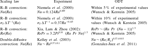
 $Nu(Ra)$ for cylindrical Rayleigh–Bénard cells with aspect ratios of 0.5–1.0. Details of the numerical simulations used to determine the model parameter values used here can be found in Wunsch & Kerstein (Reference Wunsch and Kerstein2005). That work includes tests of the ODT model for Rayleigh–Bénard convection for different parameter values and quantitative assessment of accuracy using comparisons with experimental data. It has been also used and tested carefully for the problem of double-diffusive convection where the two scalars involved were similar to the current case (e.g. Gonzalez-Juez et al. Reference Gonzalez-Juez, Kerstein and Lignell2011). Table 1 describes several examples of the comparison between the scaling results from ODT studies and relevant experimental measurements. More details about the statistical comparison between ODT results and experimental observation for different cases can be explored in the references cited above.
Comparison of scaling results from experimental studies and ODT simulations. Results shown are for Nusselt number versus  $Ra$,
 $\unicode[STIX]{x1D70E}_{T}/\unicode[STIX]{x0394}T$ versus
 $Ra$, and Reynolds number versus
 $Ra$ for single-component convection, and Nusselt number versus
 $Ra$ for double-diffusive convection. Here
 $Re$ and
 $R_{\unicode[STIX]{x1D70C}}$ are the Reynolds number based on velocity fluctuations and buoyancy ratio of two scalar components, respectively.

For this study, simulations with  $\unicode[STIX]{x0394}T$ of 6, 8, 12, 14 and 20 K and a mean of 283 K are run. All simulations have saturated bottom and top boundaries. The resulting range of Rayleigh number is
 $2.05\times 10^{8}\leqslant Ra\leqslant 2.75\times 10^{9}$. These values are similar to values that have been explored in laboratory experiments (Chandrakar et al. Reference Chandrakar, Cantrell, Chang, Ciochetto, Niedermeier, Ovchinnikov, Shaw and Yang2016; Niedermeier et al. Reference Niedermeier, Chang, Cantrell, Chandrakar, Ciochetto and Shaw2018), and they correspond to
 $Ra$ sufficiently large that the flows are fully turbulent. Moreover, the Prandtl and Schmidt number ranges used in the current simulations are
 $0.18\leqslant Pr\leqslant 0.72$ and
 $0.15\leqslant Sc\leqslant 0.72$.
3 Results and discussion
Supersaturation depends on water vapour concentration and temperature fields, so we anticipate that the magnitudes of the diffusivities for the two scalar fields will be relevant to the problem of supersaturation advection and dissipation. In order to understand the relative roles of the two diffusivities, we analyse the following four combinations throughout the rest of the paper.
(i) Actual
 $D_{v}$ and $D_{t}$: actual diffusivities for the water vapour and thermal fields, for air at a temperature of 283 K ($D_{v}/D_{t}=1.16$).
(ii)
$D_{v}=D_{t}$: the water vapour diffusivity is same as the actual thermal diffusivity ($D_{v}/D_{t}=1$).(iii)
$4\times D_{v}$: the water vapour diffusivity is four times the actual value, and the thermal diffusivity is same as the actual value ($D_{v}/D_{t}=4.63$).(iv)
$4\times D_{t}$: the water vapour diffusivity is same as the actual value, and the thermal diffusivity is four times the actual value ($D_{v}/D_{t}=0.29$).


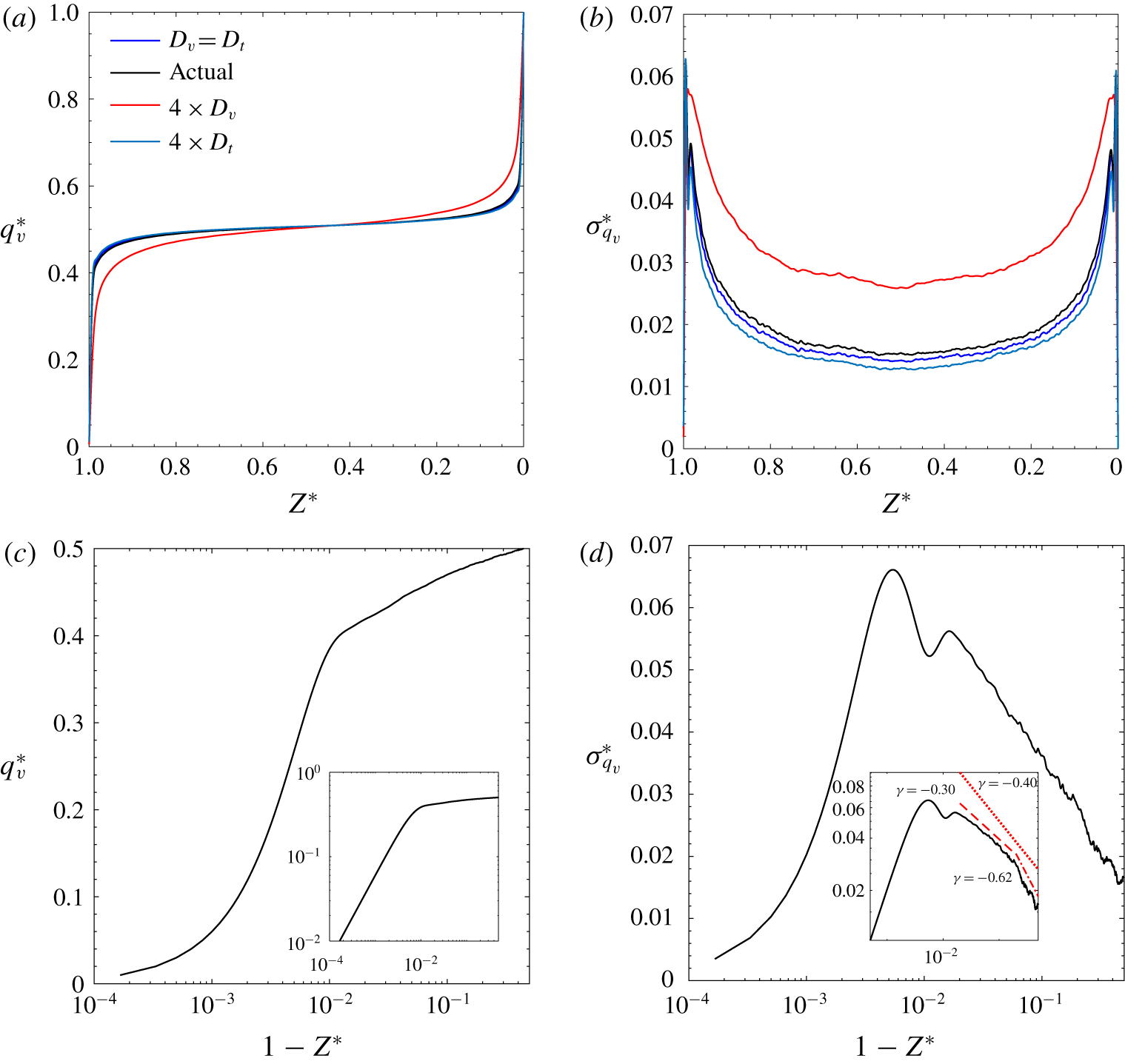
Water vapour mixing ratio mean and standard deviation profile: (a) vertical profiles of mean water vapour mixing ratio, (b) profiles of mixing ratio standard deviation for the different diffusivity cases, (c,d) semi-logarithmic plot of the scalar mean and standard deviation profiles (for the actual diffusivity case) in the half of the domain towards the cold boundary, and the inset figures are the same plots with logarithmic axis and power law ( $\propto (1-Z^{\ast })^{\unicode[STIX]{x1D6FE}}$) fittings of standard deviation. Here,
 $Z^{\ast }=0$ corresponds to the hot boundary and 1 corresponds to the cold boundary. The dotted, dashed and dash-dot curves represent power law expressions obtained from fitting the standard deviation profile outside the boundary layer at different regions.

Figure 2(a,b) illustrates the vertical profile for a single scalar field, as simulated by ODT. Specifically, it displays the mean (a) and standard deviation (b) of water vapour mixing ratio ( $q_{v}$) versus height. In the plots and rest of the text, the normalized water vapour mixing ratio and temperature variables are defined as
 $q_{v}^{\ast }=(q_{v}-q_{v_{t}})/\unicode[STIX]{x0394}q_{v}$ and
 $T^{\ast }=(T-T_{t})/\unicode[STIX]{x0394}T$. The subscripts
 $t$ and
 $b$ represent properties at the top and bottom boundaries of the domain. These profiles are consistent with results from experimental and fully resolved computational studies of R–B convection (Belmonte, Tilgner & Libchaber Reference Belmonte, Tilgner and Libchaber1993; Tilgner, Belmonte & Libchaber Reference Tilgner, Belmonte and Libchaber1993; Breuer et al. Reference Breuer, Wessling, Schmalzl and Hansen2004; Du Puits et al. Reference Du Puits, Resagk, Tilgner, Busse and Thess2007; Ahlers et al. Reference Ahlers, Bodenschatz, Funfschilling, Grossmann, He, Lohse, Stevens and Verzicco2012). Specifically, the mean scalar profile shows strong vertical gradients within the boundary layers and a relatively flat bulk profile, and the standard deviation profile shows peak variability in the boundary layers. When water vapour diffusivity is increased (the
 $4\times D_{v}$ case), the boundary layers are observed to be thicker and the standard deviation for
 $q_{v}$ is increased. These results are expected, and demonstrate the ability of ODT to capture the essential physics of the problem, i.e. the competing roles of advection and diffusion in determining scalar fluxes as a function of height. They are consistent with the findings of Wunsch & Kerstein (Reference Wunsch and Kerstein2005), who first described the ability of ODT to quantitatively represent turbulent R–B convection. Because it is a one-dimensional model, ODT does not capture processes like the formation of a large-scale circulation. In the subsequent sections we will further demonstrate the fidelity of ODT by showing comparison of fluxes with a scaling based on physical arguments.
Additionally, we have analysed the profiles of scalar mean and standard deviation outside the boundary layer, similar to Du Puits et al. (Reference Du Puits, Resagk, Tilgner, Busse and Thess2007). From figure 2(c,d), it is apparent that the mean and standard deviation profiles of water vapour mixing ratio (or temperature, not shown here) are nearly logarithmic as observed in Tilgner et al. (Reference Tilgner, Belmonte and Libchaber1993) and Ahlers et al. (Reference Ahlers, Bodenschatz, Funfschilling, Grossmann, He, Lohse, Stevens and Verzicco2012) and contrasting to the observation of power law in Du Puits et al. (Reference Du Puits, Resagk, Tilgner, Busse and Thess2007). Although, the overall exponent of the power law fitting for the standard deviation profile (inset of figure 2d) is around  $\unicode[STIX]{x1D6FE}=-0.4$, and it is very close to the value reported by Du Puits et al. (Reference Du Puits, Resagk, Tilgner, Busse and Thess2007) for the aspect ratio close to unity. In the current case, this exponent varies from
 $\unicode[STIX]{x1D6FE}=-0.3$ just outside the boundary layer to
 $\unicode[STIX]{x1D6FE}=-0.62$ near the centre of the domain. The aspect ratio close to unity is a better case for comparison considering the formulation of the ODT model structure. In ODT, the large-scale circulation is not explicitly resolved because of its dimensional constraint, although, large mapping events might incorporate the statistical features of it for the aspect ratio of unity (Wunsch & Kerstein Reference Wunsch and Kerstein2005). It is intriguing that such a simple model, ODT, can capture such details of the scalar profile in R–B convection.
3.1 Flux scaling – $Nu$ and $Sh$ as functions of $Ra_{moist}$, $Pr$ and $Sc$


Can we get the scalar fluxes in moist convection by merely extending the relation of dry convection with additional buoyancy perturbation from another scalar? Does ODT capture the effect of additional buoyancy perturbation correctly? What is the role of scalar diffusivities on the fluxes of both scalars in two-component R–B convection? These questions, along with the appropriateness of the ODT simulation for this case, are the primary motivation of this section. Dimensionless measures of heat and water vapour transfer are given by the Nusselt ( $Nu$) and Sherwood (
 $Sh$) numbers, respectively, i.e. the heat and mass transfer for turbulent convection relative to the values calculated for molecular diffusion. Conceptually, heat transfer in turbulent R–B convection is assumed to be limited by conductive heat transfer through the laminar boundary layer (BL), which itself is at a critical thickness (Howard Reference Howard1963, Reference Howard1966). This argument suggests that the Rayleigh number based on the average velocity BL thickness (
 $Ra_{\unicode[STIX]{x1D6FF}_{v}}$) is a constant parameter, such that
 $Ra_{\unicode[STIX]{x1D6FF}_{v}}/Ra=c/Ra=(\unicode[STIX]{x1D6FF}_{v}/H)^{3}$. It is also recognized that the relative thicknesses of the velocity and thermal boundary layers, for
 $Pr\sim 1$, are
 $\unicode[STIX]{x1D6FF}_{v}/\unicode[STIX]{x1D6FF}_{th}=\sqrt[]{\unicode[STIX]{x03C0}\unicode[STIX]{x1D708}t^{\ast }}/\sqrt[]{\unicode[STIX]{x03C0}D_{t}t^{\ast }}=Pr^{1/2}$. Here
 $t^{\ast }$ is a critical time scale for boundary layer development before a thermal/plume detaches from a boundary (Howard Reference Howard1966). The same argument can be extended to two-component R–B convection by replacing
 $Ra$ with
 $Ra_{moist}$, allowing the following scaling for Nusselt number to be obtained:
 $$\begin{eqnarray}Nu=\frac{H}{2\unicode[STIX]{x1D6FF}_{th}}=\frac{1}{2c^{1/3}}Pr^{1/2}Ra_{moist}^{1/3}.\end{eqnarray}$$
Similarly, the Sherwood number ( $Sh$) scaling for water vapour can be expressed as
 $$\begin{eqnarray}Sh=\frac{H}{2\unicode[STIX]{x1D6FF}_{w}}=\frac{1}{2c^{1/3}}Sc^{1/2}Ra_{moist}^{1/3},\end{eqnarray}$$
where  $\unicode[STIX]{x1D6FF}_{w}$ is the BL thickness for water vapour. For the case where
 $Pr\ll 1$, the kinematic BL is much thinner compared to the thermal BL. Therefore, the critical
 $Ra_{\unicode[STIX]{x1D6FF}_{v}}$, which is based on the stability of velocity BL, should contain the friction velocity (
 $w\sim \unicode[STIX]{x1D708}/\unicode[STIX]{x1D6FF}_{v}$) as a velocity scale. This is instead of the velocity scale determined based on the advection–diffusion balance of density, since the density change due to scalar diffusion is much smaller in the velocity BL as a result of the larger thermal BL thickness. Use of the different velocity scale leads to the following relation:
 $Ra_{\unicode[STIX]{x1D6FF}_{v}}/Ra_{moist}=c/Ra_{moist}=Pr^{-1}(\unicode[STIX]{x1D6FF}_{v}/H)^{3}$. Consequently, we obtain the following modified scalings for
 $Nu$ and
 $Sh$:
 $$\begin{eqnarray}\displaystyle & \displaystyle Nu=\frac{H}{2\unicode[STIX]{x1D6FF}_{th}}=\frac{H}{2\unicode[STIX]{x1D6FF}_{v}}\frac{\unicode[STIX]{x1D6FF}_{v}}{\unicode[STIX]{x1D6FF}_{th}}=\frac{1}{2c^{1/3}}Pr^{1/6}Ra_{moist}^{1/3}, & \displaystyle\end{eqnarray}$$
 $$\begin{eqnarray}\displaystyle & \displaystyle Sh=\frac{H}{2\unicode[STIX]{x1D6FF}_{w}}=\frac{H}{2\unicode[STIX]{x1D6FF}_{v}}\frac{\unicode[STIX]{x1D6FF}_{v}}{\unicode[STIX]{x1D6FF}_{w}}=\frac{1}{2c^{1/3}}Sc^{1/2}Pr^{-1/3}Ra_{moist}^{1/3}. & \displaystyle\end{eqnarray}$$
The above simplified scalings are based on the foundation of Howard (Reference Howard1963, Reference Howard1966) and a linear BL approximation for the heat flux estimation. Moreover, any effects of turbulent fluctuations (or eddies) at the edge of BL in the boundary layer heat transport are ignored. A more detailed treatment of the scaling relations likely can be obtained by extending the Grossmann & Lohse (Reference Grossmann and Lohse2000, Reference Grossmann and Lohse2004) theory to the two-component RB convection problem. For the current purposes, however, where the goal is to understand the essential features of the supersaturation field within moist convection, we stay with this simplified treatment of the scaling relations.
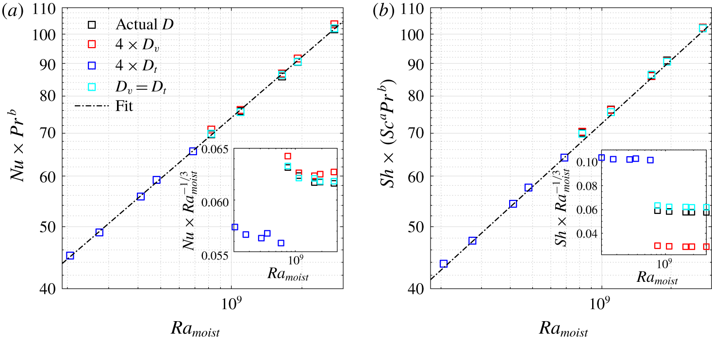
Variation of the scalar fluxes of heat ( $Nu$) and water vapour (
 $Sh$) with moist Rayleigh number (
 $Ra_{moist}$): (a)
 $Nu$ scaled with
 $Pr$ according to the scaling relations (3.1) and (3.3) and plotted against
 $Ra_{moist_{t}}$, (b)
 $Sh$ scaled with
 $Sc$ and
 $Pr$ according to the scaling relations (3.2) and (3.4) and plotted against
 $Ra_{moist}$. Inset figures are the compensated plots where
 $Nu$ and
 $Sh$ are multiplied with
 $Ra_{moist}^{-1/3}$ and plotted against
 $Ra_{moist}$. Fittings of the scaled
 $Nu$ and
 $Sh$ data produce
 $Ra_{moist}$ exponents around
 $0.316\pm 0.005$ and
 $0.328\pm 0.006$.

Figure 3 demonstrates the Nusselt (a) and Sherwood (b) number scaling with  $Ra_{moist}$ as produced by ODT, and serves as a check for the
 $Nu$ and
 $Sh$ scalings described above. It is apparent from the collapse of the data points to a line that the
 $Nu$ scalings ((3.1) and (3.3)) and
 $Sh$ scalings ((3.2) and (3.4)) reasonably describe the heat and water vapour fluxes for the simulated ranges of
 $Pr$ and
 $Sc$. Moreover, fittings of the scaled
 $Nu$ and
 $Sh$ produce
 $Ra_{moist}$ exponents of
 $0.316\pm 0.005$ and
 $0.328\pm 0.006$ for heat and water vapour scalars, respectively. The compensated plots, as shown in inset figures, also display nearly a flat response with
 $Ra_{moist}$. However, there is a slight negative slope in the compensated
 $Nu$ plot, which explains the somewhat lower exponent than
 $1/3$. These exponents are close to
 $1/3$ and previous experimental results (Niemela et al. Reference Niemela, Skrbek, Sreenivasan and Donnelly2000; Fleischer & Goldstein Reference Fleischer and Goldstein2002; Niemela & Sreenivasan Reference Niemela and Sreenivasan2006). Similarly, the
 $Pr$ scaling presented in numerical studies by Verzicco & Camussi (Reference Verzicco and Camussi1999) and Breuer et al. (Reference Breuer, Wessling, Schmalzl and Hansen2004) for the low
 $Pr$ case are also roughly consistent with the scaling exponent presented here (
 $1/6$). These results build confidence in the scaling, as well as in the ability of ODT to reproduce essential statistics of R–B convection.
3.2 Scalar fluctuations in the bulk fluid
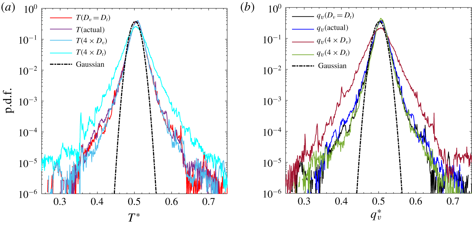
The p.d.f.s of (a) temperature and (b) water vapour fluctuations near the domain centre for the different diffusivity cases (8 K applied temperature difference). The dot-dashed line is a Gaussian curve fit to the scalar p.d.f. for the actual diffusivity case.

The central purpose of this section is first to confirm that the behaviour of scalar statistics in the bulk region are in line with expected behaviour. Then we extended the analysis to explore the role of differential diffusivity, and ultimately the implications for temperature-water vapour covariance, which is crucial for determining supersaturation statistics.
In the bulk fluid in turbulent R–B convection, scalar fluctuations are determined by turbulent scalar advection from the BL and destruction of scalar gradients due to the molecular diffusion. Therefore, the magnitude of scalar fluctuations in the bulk fluid is not just a function of the applied buoyancy forcing through  $\unicode[STIX]{x0394}T$, but it also depends on the diffusivity of the scalar. Figure 4 demonstrates this concept, that the scalar diffusivity is important in determining the bulk fluctuations. It displays p.d.f.s of water vapour and temperature fluctuations near the centre of the domain. Apparently, the dispersion of the scalar p.d.f. is larger when its diffusivity is higher. The dot-dashed lines in the plots show a Gaussian curve fit of the scalar p.d.f. for the actual diffusivity case. From the comparison with the curve fit, it is clear that far tails of the distributions have a slower decay than the Gaussian, in fact nearly exponential tails, as expected at the centre of a turbulent R–B convection cell. Moreover, tails deviate further from Gaussian with an increase in diffusivities of the scalar. Therefore, the dispersion of the scalar p.d.f. increases with increase in respective scalar diffusivities. Moreover, all scalar p.d.f.s from the centre of the domain are nearly symmetric as expected and become more skewed closer to the boundaries (not shown here). Can we extend a previously reported scaling approach for scalar variance in one component convection (for example, Castaing et al. (Reference Castaing, Gunaratne, Heslot, Kadanoff, Libchaber, Thomae, Wu, Zaleski and Zanetti1989)) to the moist (or two component) convection case, including an explanation for why
 $\unicode[STIX]{x1D70E}_{T}$ and
 $\unicode[STIX]{x1D70E}_{q_{v}}$ tend to change with
 $Ra_{moist}$,
 $Pr$, and
 $Sc$? Additionally, do ODT results support these scaling relations? We consider these questions in the remainder of this section.
A simplified relation for the bulk fluctuation with moist-convection parameters ( $Ra_{moist}$,
 $Sc$ and
 $Pr$) can be derived based on scaling arguments similar to Castaing et al. (Reference Castaing, Gunaratne, Heslot, Kadanoff, Libchaber, Thomae, Wu, Zaleski and Zanetti1989). During steady moist-convection, the bulk convective acceleration (
 $w\unicode[STIX]{x2202}w/\unicode[STIX]{x2202}z$) is mainly supported by the buoyancy forcing in the bulk fluid (
 $g\unicode[STIX]{x1D6FD}\unicode[STIX]{x1D6FF}T_{v,bulk}$), and the viscous force is negligible unless the length scale of interest is very small. If the buoyancy contribution of water vapour is small, the bulk virtual temperature difference (
 $\unicode[STIX]{x1D6FF}T_{v,bulk}$) can be approximated from the mean temperature profile. The mean virtual temperature drop in the bulk flow can be approximated as
 $\unicode[STIX]{x1D705}\unicode[STIX]{x0394}T_{v}$ based on the assumption of Howard’s boundary layer profile (Howard Reference Howard1966), where the constant of proportionality
 $\unicode[STIX]{x1D705}$ depends on
 $Pr$ and
 $Sc$. Additionally,
 $\unicode[STIX]{x1D705}\ll 1$ since most of the temperature drop occurs in the boundary layers. Consequently, we get the following scaling relation for the normalized vertical-velocity fluctuation (
 $\unicode[STIX]{x1D70E}_{w}^{\ast }\equiv \unicode[STIX]{x1D70E}_{w}H/D_{t}$) in the bulk:
 $$\begin{eqnarray}\unicode[STIX]{x1D70E}_{w}^{\ast }\sim \unicode[STIX]{x1D705}^{1/2}~Ra_{moist}^{1/2}Pr^{1/2}\left(\frac{z}{H}\right)^{1/2}.\end{eqnarray}$$
The heat and water vapour transport in the bulk are due to both the turbulent convection and the diffusion as a result of the mean scalar gradient. In the limit of low  $Pr$ or
 $Sc$, the diffusion term in the heat or water vapour flux can be neglected. As a result,
 $Nu$ and
 $Sh$ can be approximated as
 $\overline{w^{\prime }T^{\prime }}^{\ast }$ and
 $\overline{w^{\prime }q_{v}^{\prime }}^{\ast }$, and the order of these terms can be represented as
 $\unicode[STIX]{x1D70E}_{w}^{\ast }\unicode[STIX]{x1D70E}_{T}^{\ast }$ and
 $\unicode[STIX]{x1D70E}_{w}^{\ast }\unicode[STIX]{x1D70E}_{q_{v}}^{\ast }Pr^{-1}Sc$, respectively. Here,
 $\unicode[STIX]{x1D70E}_{T}^{\ast }\equiv \unicode[STIX]{x1D70E}_{T}\unicode[STIX]{x0394}T^{-1}$ and
 $\unicode[STIX]{x1D70E}_{q_{v}}^{\ast }\equiv \unicode[STIX]{x1D70E}_{q_{v}}\unicode[STIX]{x0394}q_{v}^{-1}$. By using the
 $Nu$ and
 $Sh$ scaling from equations (3.1) and (3.2), the following scalings for the normalized scalar fluctuations can be derived:
 $$\begin{eqnarray}\unicode[STIX]{x1D70E}_{T}^{\ast }\sim \unicode[STIX]{x1D705}^{-1/2}Ra_{moist}^{-1/6}\left(\frac{z}{H}\right)^{-1/2}\end{eqnarray}$$
and
 $$\begin{eqnarray}\unicode[STIX]{x1D70E}_{q_{v}}^{\ast }\sim \unicode[STIX]{x1D705}^{-1/2}~Ra_{moist}^{-1/6}Sc^{-1/2}Pr^{1/2}\left(\frac{z}{H}\right)^{-1/2}.\end{eqnarray}$$
If  $Pr\ll 1$, the above scalings for the temperature fluctuation will not be applicable since there will be a significant contribution of the heat flux due to the temperature gradient in the bulk, as well as the scaling for
 $Nu$ being different. Moreover, the correlation between temperature and vertical velocity will be reduced because of a significantly larger diffusivity of the thermal field. Due to a similar reason as the
 $Pr\ll 1$ case, for the
 $Sc\ll 1$ case (3.7) will also not be applicable. Evidence for a higher mean gradient in the bulk for the
 $Sc\ll 1$ case is manifested in figure 2. For the
 $Pr\ll 1$ case, however, a new scaling of
 $\unicode[STIX]{x1D70E}_{qv}^{\ast }$ can be obtained, and it is slightly different than (3.7) due to the different flux scaling in (3.4),
 $$\begin{eqnarray}\unicode[STIX]{x1D70E}_{q_{v}}^{\ast }\sim \unicode[STIX]{x1D705}^{-1/2}Ra_{moist}^{-1/6}Sc^{-1/2}Pr^{1/6}\times \left(\frac{z}{H}\right)^{-1/2}.\end{eqnarray}$$
Although, as explained above that the scaling for  $\unicode[STIX]{x1D70E}_{T}^{\ast }$ (for
 $Pr\ll 1$ ) and
 $\unicode[STIX]{x1D70E}_{qv}^{\ast }$ (for
 $Sc\ll 1$) derived based on the
 $Nu/Sh$ relation may not be completely applicable due to a non-negligible mean scalar gradient in the bulk as well as a decrease in correlation efficiency between vertical velocity and scalar fluctuations, we still present these results below for the completeness of the discussion;
 $$\begin{eqnarray}\unicode[STIX]{x1D70E}_{T}^{\ast }\sim \unicode[STIX]{x1D705}^{-1/2}Ra_{moist}^{-1/6}~Pr^{-1/3}\left(\frac{z}{H}\right)^{-1/2}\end{eqnarray}$$
and
 $$\begin{eqnarray}\unicode[STIX]{x1D70E}_{q_{v}}^{\ast }\sim \unicode[STIX]{x1D705}^{-1/2}Ra_{moist}^{-1/6}Sc^{-1/2}Pr^{1/2}\left(\frac{z}{H}\right)^{-1/2}.\end{eqnarray}$$
For these cases, the actual  $Pr/Sc$ exponent might be slightly different from above scaling relations for the actual
 $Pr\sim 1$ and
 $Sc\sim 1$ ranges.
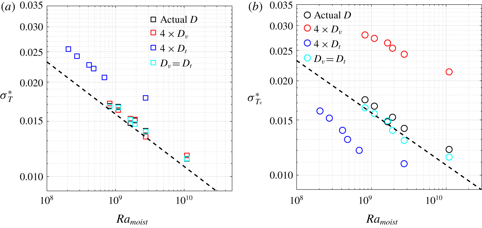
Normalized standard deviations of (a) temperature and (b) water vapour ( $\unicode[STIX]{x1D70E}_{T}^{\ast }\equiv \unicode[STIX]{x1D70E}_{T}\unicode[STIX]{x0394}T^{-1}$ and
 $\unicode[STIX]{x1D70E}_{q_{v}}^{\ast }\equiv \unicode[STIX]{x1D70E}_{q_{v}}\unicode[STIX]{x0394}q_{v}^{-1}$) near the domain centre versus
 $Ra_{moist}$. The dashed line represents the
 $Ra_{moist}^{-1/6}$ scaling from (3.6) and (3.7).

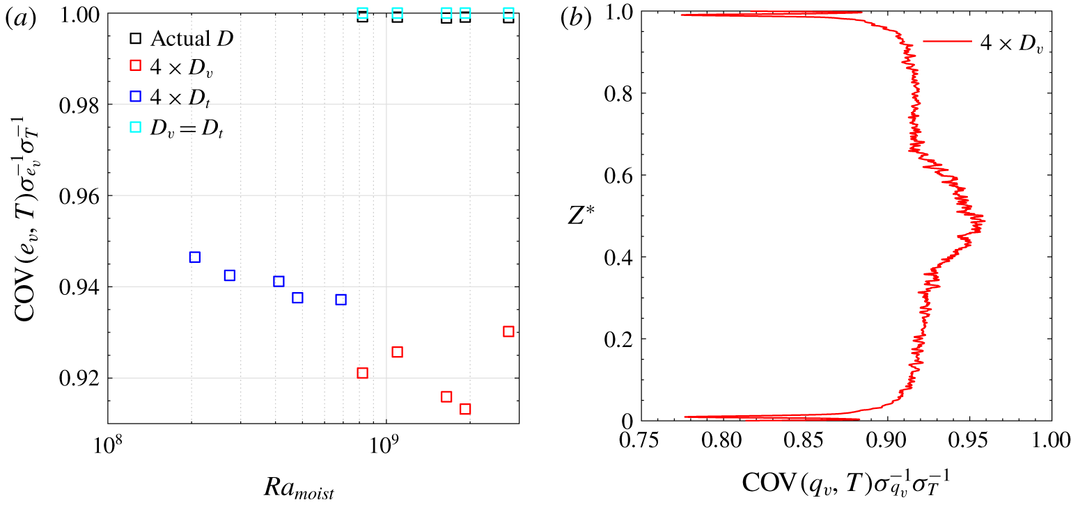
(a) Normalized covariance of temperature and water vapour pressure at the domain centre versus  $Ra_{moist}$. (b) An example of the vertical profile of normalized covariance of temperature and water vapour mixing ratio across the domain for 20 K applied temperature difference (and for the case where water vapour diffusivity is four times the actual value).

Figure 2 illustrates that the scaling presented above qualitatively represents the shape of the scalar fluctuation profile outside the BL. The normalized  $q_{v}$ standard deviation decreases nearly in a parabolic profile outside the BL, consistent with scaling. The derived power of
 $Ra_{mosit}$ in the above scalings is close to the experimentally observed
 $\unicode[STIX]{x1D70E}_{T}^{\ast }-Ra$ scaling for single-component R–B convection (Niemela et al. Reference Niemela, Skrbek, Sreenivasan and Donnelly2000), as well as to predictions of Grossmann & Lohse (Reference Grossmann and Lohse2000, Reference Grossmann and Lohse2004).
Similarly, as expected from the scaling relations, figure 5 displays a decreasing trend of the normalized standard deviation of  $T$ and
 $q_{v}$ with
 $Ra_{moist}$. Furthermore, the
 $Ra_{moist}$ exponent obtained from a data fit is close to the prediction from the scaling law, as can be seen from the dashed reference lines with (
 $-1/6$) slope. For the low-
 $Pr$ case, the
 $\unicode[STIX]{x1D70E}_{T}^{\ast }$ data points are slightly offset from the normal trend of the other data set; this is due to the additional
 $Pr$ dependency because of a higher thermal diffusivity as explained in the earlier paragraphs (3.9). Likewise, for the same case,
 $\unicode[STIX]{x1D70E}_{qv}^{\ast }$ data points are slightly lower, as expected from the scaling relation (3.8) due to the
 $Pr^{1/6}$ dependence. Moreover, with a decrease of
 $Sc$, i.e. an increase of the water vapour diffusivity, the normalized water vapour fluctuation increases as anticipated by the scaling relation. Although, for the
 $Sc\ll 1$ case, the
 $Sc$ dependency in the relation (3.7) will be slightly different due to a significant mean gradient in the bulk as explained earlier.
The covariance of other scalars with the temperature field in convective flows is an important quantity for atmospheric applications since it is related to the reaction rate or rate of phase change through the supersaturation. Figure 6(a) shows the normalized covariance of water vapour pressure and temperature at the centre of the convection cell, as a function of  $Ra_{moist}$. As anticipated, it is close to one for the cases with small diffusivity difference. However, for higher diffusivity differences, it drops down slightly. In these cases, the normalized covariance decreases with an increase in the buoyancy forcing (
 $Ra_{moist}$). As depicted in figure 6(b), the covariance magnitude also varies along a vertical profile moving towards boundaries, due to the higher effect of relative diffusion and lower turbulence level closer to the boundaries. In cumulus clouds, the normalized covariance between temperature and water vapour field was estimated between 0.24 and 0.34 using high-frequency measurements of temperature and water vapour concentration (Siebert & Shaw Reference Siebert and Shaw2017). These values are significantly lower than the current simplistic case. It should be noted, however, that in cloudy convection the presence of water vapour and heat fluxes resulting from entrainment and condensation could decrease this covariance further from the idealized confined convection case.
3.3 From two scalars to supersaturation: mixing diagrams and vertical profiles
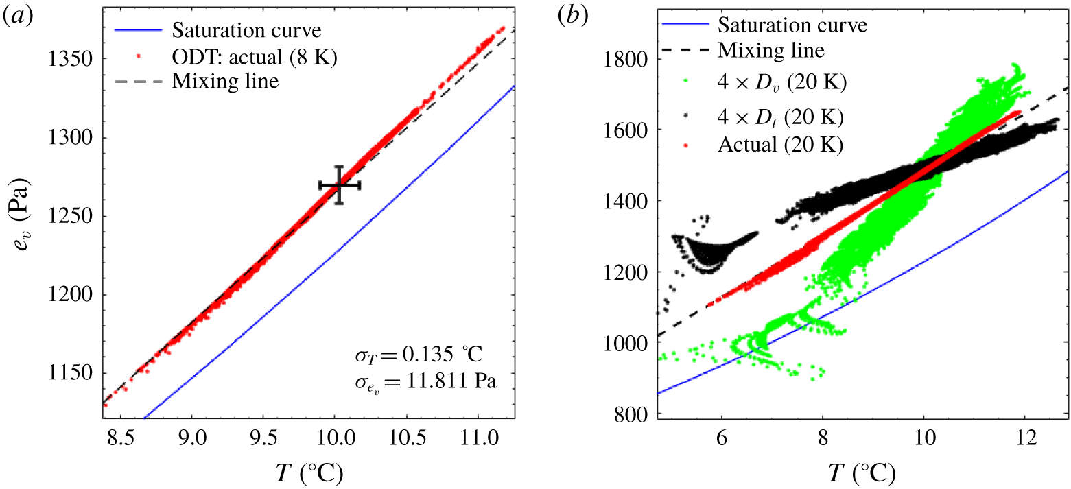
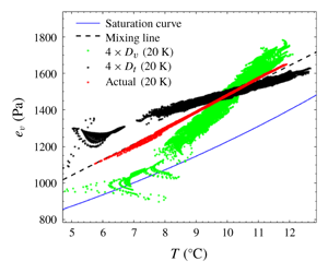
(a) An example of the mixing diagram for the actual diffusivity case at 8 K applied temperature difference with error bars showing standard deviation. (b) Mixing diagram for different diffusivity cases at a higher applied temperature difference (20 K).

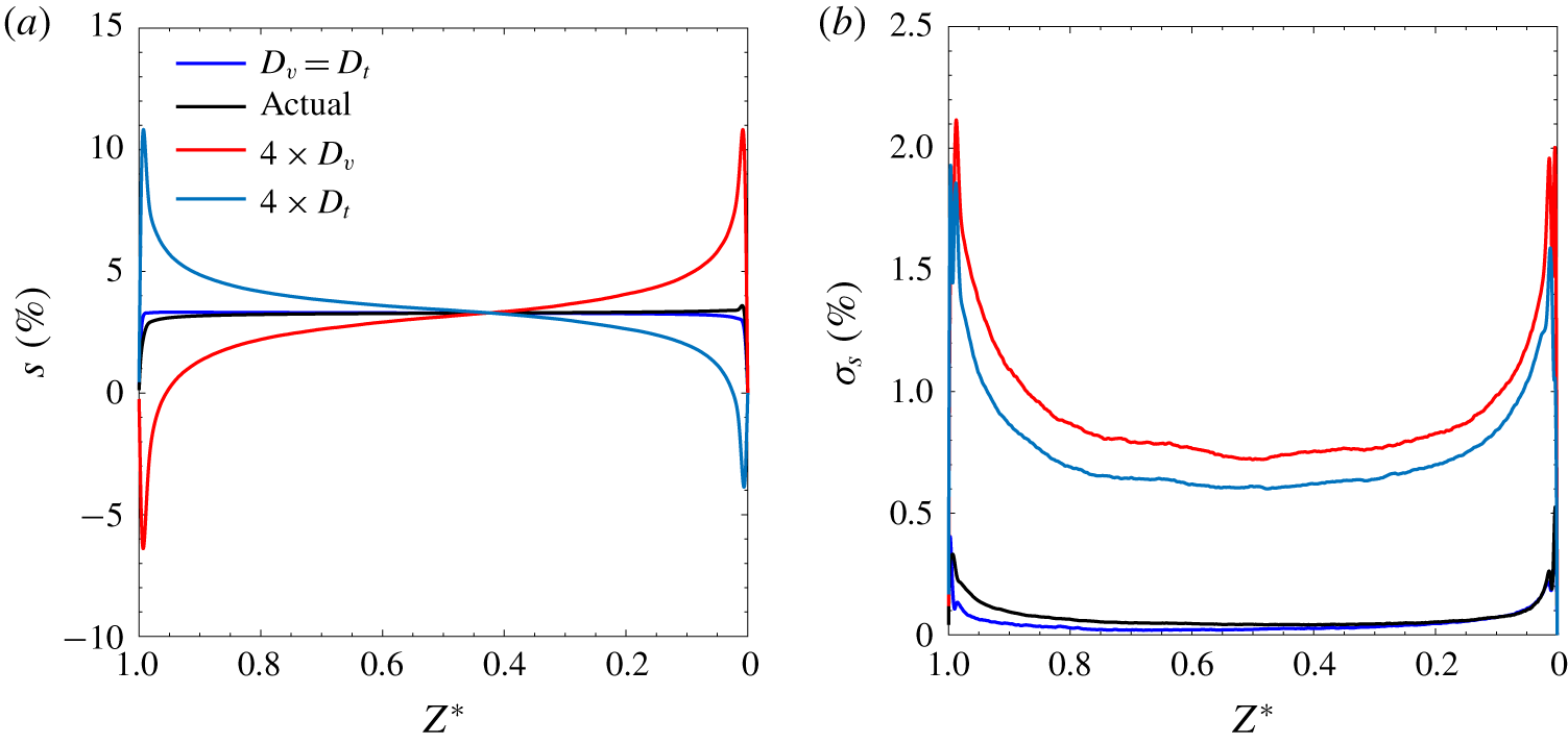
Supersaturation mean and fluctuation profile: (a) vertical profiles of the supersaturation mean, (b) Profiles of supersaturation fluctuations (standard deviations) for the different diffusivity cases. (Here,  $Z^{\ast }=0$ corresponds to the hot boundary and 1 corresponds to the cold boundary.)

In atmospheric R–B convection the relevant scalar for cloud formation is the supersaturation, which as discussed already is a combination of the two scalars, water vapour pressure and temperature:  $s\equiv (e_{v}/e_{v,s}(T))-1$. The saturation value
 $e_{v,s}(T)$ is related exponentially to the temperature through the Clausius–Clapeyron equation. We note that water vapour pressure and water vapour mixing ratio can be considered as interchangeable, via the ideal gas law. In figure 2 and § 3.2 we considered the vertical profiles and fluctuations of the two individual scalars, and in this subsection we extend to supersaturation. In the following two subsections we then investigate the bulk and boundary-layer properties of supersaturation in more detail.
Figure 7 shows mixing diagrams obtained from ODT grid points near the centre of the domain. As discussed in the introduction, in an idealized scenario one would expect the sampled values of  $e_{v}$ and
 $T$ to lie along a linear mixing line (dashed curve). In figure 7(a), which corresponds to
 $\unicode[STIX]{x0394}T=8~\text{K}$ and for the actual diffusivities, this can be seen to be approximately true. In figure 7(b), however, corresponding to
 $\unicode[STIX]{x0394}T=20~\text{K}$, it can be seen that for the two cases with different scalar diffusivities, the points deviate from the idealized mixing line. When the thermal diffusivity is higher than the water vapour, the cloud of points spreads more strongly along the temperature axis and therefore has a shallower slope than the mixing line. This is due to a higher relative transport for the temperature compared to the water vapour due to its higher diffusivity. The exact opposite argument is also valid when considering higher water vapour diffusivity. The spread of points is now greater along the vapour pressure axis leading to a steeper inclination compared to the mixing line. We can anticipate that this higher spread produces greater fluctuations in supersaturation relative to the idealized mixing scenario with nearly equal diffusivities (cf. § 3.4). The relative supersaturation fluctuation can be visualized by comparing the spread of data points above and below the saturation curve.
Supersaturation mean and fluctuation profiles in the atmospheric boundary-layer are anticipated to be relevant for cloud microphysical processes and dynamics. Figure 8 illustrates the profile of supersaturation mean (a) and standard deviation (b) ( $\unicode[STIX]{x1D70E}_{s}$) across the domain. The mean supersaturation profile is nearly flat in the bulk fluid, just for the individual scalars, when the diffusivity difference is small. For these cases, it is also close to the mean value one calculates from the idealized mixing process. Interestingly, the slope of the mean supersaturation profile flips sign in both halves of the domain when one of the scalar diffusivities is significantly higher than the other. Moreover, a difference in the scalar diffusivities causes a significant peak to appear in the mean supersaturation profile, close to the boundaries. Which diffusivity is larger also determines the sign of the supersaturation (or subsaturation) peak near the two boundaries. If the thermal diffusivity is higher than the water vapour diffusivity, the supersaturation peak is positive at the cold boundary and negative at the hot boundary (and opposite otherwise). A higher diffusivity of a scalar leads to a smaller slope of the mean scalar profile in the boundary layer. Therefore, if the thermal diffusivity is higher than the other scalar, the drop in average temperature from the hot boundary is slower than the case when both are equal. As a result of the above effect as well as the exponential relation of the saturation vapour pressure with temperature, the supersaturation profile produces a negative peak close to the hot boundary and a positive peak near the cold boundary for a higher thermal diffusivity and opposite otherwise. Additionally, for the higher relative diffusivity cases, the mean profile does not cross the mean value and each other precisely at
 $Z^{\star }=0.5$, due to the nonlinear relation of saturation vapour pressure with temperature (the Clausius–Clapeyron equation). The saturation vapour pressure change is not symmetric at a temperature lower or higher than the mean because of this nonlinearity. Similarly, the multiple peaks in standard deviation profiles near the boundaries could also be a result of this nonlinearity since it does not exist (only one peak) in the temperature or water vapour mixing ratio profiles. The
 $\unicode[STIX]{x1D70E}_{s}$ profile responds analogously to the individual scalar profiles (cf. figure 2); i.e. it peaks near the boundaries and decreases while approaching the centre. This decreasing response with
 $Z^{\star }$ is qualitatively consistent with the parabolic decrease found in § 3.4 for scaling of supersaturation in the bulk fluid. Furthermore, in that subsection we also investigate the observation that
 $\unicode[STIX]{x1D70E}_{s}$ increases significantly for the cases with different scalar diffusivities.
3.4 Supersaturation fluctuations in the bulk fluid: contributions from both scalars
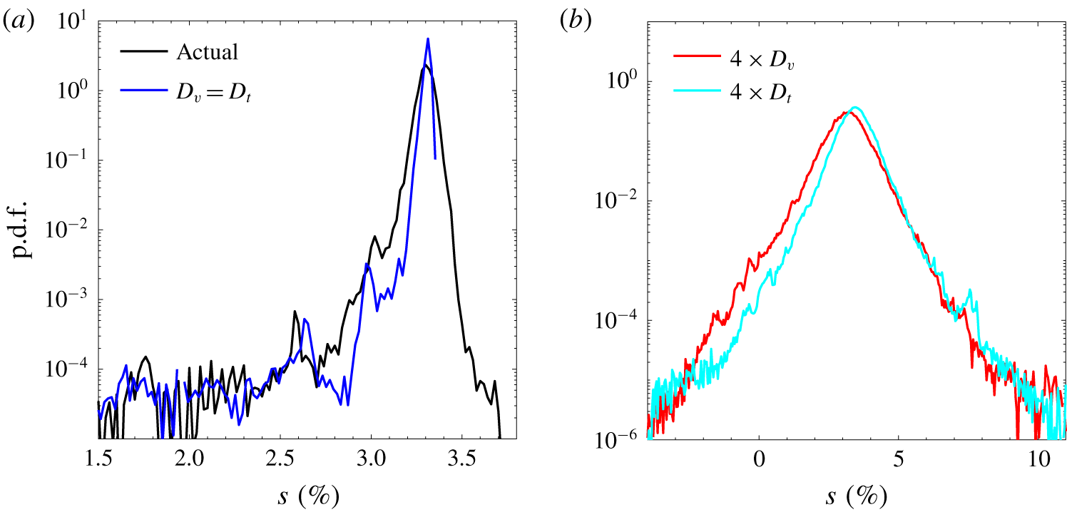
Sample p.d.f.s of supersaturation near the domain centre for the different diffusivity cases (8 K applied temperature difference).

In this subsection we consider the behaviour of supersaturation fluctuations in the bulk fluid, away from the BL. Figure 9 shows several examples of supersaturation p.d.f.s for different thermal and water vapour diffusivity combinations. Analogous to the temperature and vapour mixing ratio p.d.f.s, it responds to a change in the diffusivity of both scalars. However, it produces broader p.d.f.s with an increase in the difference in diffusivity of water vapour and temperature (not the absolute diffusivities of both scalars) due to the nonlinear coupling of both scalars in supersaturation. Moreover, figure 9 shows that the p.d.f.s are negatively skewed for the lower relative diffusivity cases (figure 9a). This negative skewness of the fluctuation distribution is due to the increasing slope of the saturation curve with temperature (i.e. the exponential temperature dependence).
As described earlier, both scalar fluctuations (normalized by the applied scalar gradients) can be scaled as a function of  $Ra_{moist}$,
 $Pr$ and
 $Sc$. Therefore, we expect that the supersaturation fluctuation can also be scaled as a function of these parameters. A detailed exploration of the contributions from both scalars can be made by expressing supersaturation variance as a function of temperature and water vapour pressure variances (Kulmala et al. Reference Kulmala, Rannik, Zapadinsky and Clement1997; Siebert & Shaw Reference Siebert and Shaw2017),
 $$\begin{eqnarray}\unicode[STIX]{x1D70E}_{s}^{2}\approx S^{2}\left[\left(\frac{\unicode[STIX]{x1D70E}_{e_{v}}}{\bar{e_{v}}}\right)^{2}+\unicode[STIX]{x1D701}^{2}\left(\frac{\unicode[STIX]{x1D70E}_{T}}{\bar{T}}\right)^{2}-2\unicode[STIX]{x1D701}\frac{\overline{T^{\prime }e_{v}^{\prime }}}{\bar{T}\bar{e_{v}}}\right].\end{eqnarray}$$
Here,  $S=e_{v}/e_{v,s}(\bar{T})$ is the mean saturation ratio,
 $e_{v,s}(\bar{T})$ is the saturation vapour pressure at temperature the average temperature, and
 $\unicode[STIX]{x1D701}={\mathcal{L}}/(R_{v}\bar{T})$. Additionally, primes and bars represent fluctuations and mean quantities, respectively.
With the use of the scaling expressions (3.6) and (3.7), a linearized form of the Clausius–Clapeyron equation ( $\unicode[STIX]{x0394}e_{v,s}\approx \unicode[STIX]{x1D701}\bar{e}_{v,s}\unicode[STIX]{x0394}T/\bar{T}$), and (3.11), the following scaling relation for supersaturation fluctuations can be obtained:
 $$\begin{eqnarray}\left(\frac{\unicode[STIX]{x1D70E}_{s}}{S}\right)^{2}\sim \unicode[STIX]{x1D705}^{-1}\unicode[STIX]{x1D709}^{2}\left[1+\frac{Pr}{S^{2}Sc}-\frac{2C_{q_{v},T}}{S}\left(\frac{Pr}{Sc}\right)^{1/2}\right]Pr^{-2}Ra_{moist}^{5/3}\left(\frac{z}{H}\right)^{-1}.\end{eqnarray}$$
Here,  $C_{q_{v},T}$ is the correlation efficiency of water vapour mixing ratio and temperature and
 $\unicode[STIX]{x1D709}=\unicode[STIX]{x1D701}\unicode[STIX]{x1D708}^{2}/gH^{3}$. As can be seen from figure 6, the correlation efficiency of water vapour and temperature fluctuations reside mostly in the neighbourhood of 100 %, at least for the current range of
 $Ra_{moist}$. With this information, equation (3.12) can be simplified to
 $$\begin{eqnarray}\left(\frac{\unicode[STIX]{x1D70E}_{s}}{S}\right)^{2}\sim \unicode[STIX]{x1D705}^{-1}~\unicode[STIX]{x1D709}^{2}\left[1-\frac{1}{S}\left(\frac{Pr}{Sc}\right)^{1/2}\right]^{2}Pr^{-2}Ra_{moist}^{5/3}\left(\frac{z}{H}\right)^{-1}.\end{eqnarray}$$
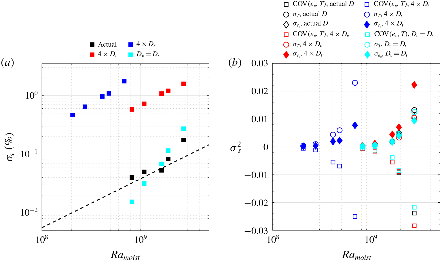
Figure 10(a) displays the variation of supersaturation fluctuations with  $Ra_{moist}$ as a result of fluctuations in both scalars. There is an increasing trend of the supersaturation fluctuations with
 $Ra_{moist}$ as anticipated from the scaling relation (3.12), and as indicated by the dashed line with the predicted scaling slope for
 $Ra_{moist}$. The magnitude of
 $\unicode[STIX]{x1D70E}_{s}$ is larger for a higher difference between the water vapour and thermal diffusivity. This effect of diffusivity difference on
 $\unicode[STIX]{x1D70E}_{s}$ is also predicted by the scaling relation (3.13). Contributions of the different terms of (3.11) to the magnitude of the supersaturation fluctuations are shown in figure 10(b). It can be seen that all terms are equally important, although because of the strong covariance, (3.11) can be further simplified by replacing the covariance term with the standard deviations of the two scalars. Moreover, the scalar with a higher diffusivity dominates the contribution, and the covariance term always has the largest magnitude.
Supersaturation fluctuation statistics at the domain centre. (a) Supersaturation standard deviation as a function of  $Ra_{moist}$ and its comparison between the different diffusivity cases. The dashed line represents the
 $Ra_{moist}^{5/6}$ scaling from (3.13). (b) Contributions of different scalar statistics (as shown in (3.11)) to the supersaturation variance versus
 $Ra_{moist}$.

3.5 Supersaturation profiles in the boundary layer
In this subsection we move from the bulk to the boundary layer. The mean and instantaneous BL profiles in R–B convection have been observed to be close to the BL theory of Prandtl–Blasius–Pohlhausen (Zhou & Xia Reference Zhou and Xia2010; Zhou et al. Reference Zhou, Stevens, Sugiyama, Grossmann, Lohse and Xia2010). Therefore, to explore the supersaturation profile within the boundary layer, we have used the Prandtl–Blasius–Pohlhausen profiles for the water vapour and temperature fields. As mentioned above, some studies claim the Prandtl–Blasius–Pohlhausen profile reasonably represents the scalar profile in the boundary layer of single-component Rayleigh–Bénard convection. In the current case, even though we have two driving scalars and the air is supersaturated with water vapour, both scalars contribute to positive buoyancy, avoiding the complexities of double-diffusive convection. In fact, the moist convection case can be expressed as single-component R–B convection with the virtual temperature difference as the driving scalar. The only complication arises due to the different diffusivities of both scalars, which changes the relative slopes of the two profiles. However, the concept of the Prandtl–Blasius–Pohlhausen profile due to the large-scale circulation can also be extended for this case since two scalars do not have contrasting buoyancy contributions, unlike in double-diffusive convection. Its applicability may be questioned even in the case of the single-component R–B convection due to the presence of the plume structure near boundaries. Therefore, we also have compared this profile with Howard’s model (Howard Reference Howard1966) to explore the supersaturation profile.
With the assumption of low  $Pr/Sc$ (i.e. the thermal and water vapour boundary layer completely encapsulates the velocity boundary layer), we can obtain a simplified solution of the water vapour and thermal boundary layer. This assumption (
 $\unicode[STIX]{x1D6FF}_{v}<\unicode[STIX]{x1D6FF}_{th}$ and
 $\unicode[STIX]{x1D6FF}_{v}<\unicode[STIX]{x1D6FF}_{w}$) might be a reasonable approximation for the
 $Pr/Sc$ range considered in this study. It implies that the velocity variation in the thermal or water vapour boundary layer is neglected. Since the Blasius boundary layer is expected to be self-similar, using a similarity transform with similarity variables
 $\unicode[STIX]{x1D702}=z/\unicode[STIX]{x1D6FF}(x)$,
 $\unicode[STIX]{x1D6E9}=2(T_{b}-T)/\unicode[STIX]{x0394}T$ and
 $\unicode[STIX]{x1D713}=U\unicode[STIX]{x1D6FF}(x)f(\unicode[STIX]{x1D702})$ (or
 $f^{\prime }(\unicode[STIX]{x1D702})=u(z)/U$), a simplified solution can be obtained (Schlichting et al. Reference Schlichting, Gersten, Krause, Oertel and Mayes1955; Bejan Reference Bejan2013)
 $$\begin{eqnarray}\unicode[STIX]{x1D6E9}(\unicode[STIX]{x1D702})=\text{erf}\left(\frac{\unicode[STIX]{x1D702}~\sqrt[]{Pr}}{2}\right).\end{eqnarray}$$
Here  $\unicode[STIX]{x1D713}$,
 $\unicode[STIX]{x1D6FF}$,
 $T_{b}$ and
 $U$ are the velocity stream-function, BL thickness, temperature at the bottom boundary and free stream velocity, respectively. This solution is also applicable for the water vapour field with corresponding changes in variables (e.g.
 $Pr$ replaced with
 $Sc$ and
 $\unicode[STIX]{x1D6FF}_{th}$ with the BL thickness for water vapour,
 $\unicode[STIX]{x1D6FF}_{w}$). The streamwise velocity scale
 $U$ determines the time scale for the boundary layer growth, i.e. the kinematic boundary layer thickness at location
 $x$ from the leading edge scales as
 $\sqrt{\unicode[STIX]{x1D708}\unicode[STIX]{x1D70F}}$, where
 $\unicode[STIX]{x1D70F}=x/U$. For Rayleigh–Bénard convection, the streamwise velocity is thought to be a result of the large-scale circulation, which is still questionable due to the presence of the intermittent plume structure near boundaries. The plume structure of the boundary layer suggests that the intermittent boundary layer develops locally until a plume detaches from the boundary. In ODT simulations the large-scale circulation is not represented explicitly due to its one-dimensional structure; however, the effect of a large-scale circulation is represented stochastically by the large-scale mappings (Wunsch & Kerstein Reference Wunsch and Kerstein2005). Therefore, for the completeness of the discussion, we have included the Prandtl–Blasius–Pohlhausen solution of the thermal and water vapour profiles. The thermal BL thickness can be estimated from
 $\unicode[STIX]{x1D6FF}_{th}=H/(2~Nu)$ together with the
 $Nu{-}Ra$ relation. We use the above solution in conjunction with the empirical relation of
 $Nu$ and
 $Sh$ from fitting (as explored in § 3.1) and the Clausius–Clapeyron equation to get the BL profile of supersaturation.
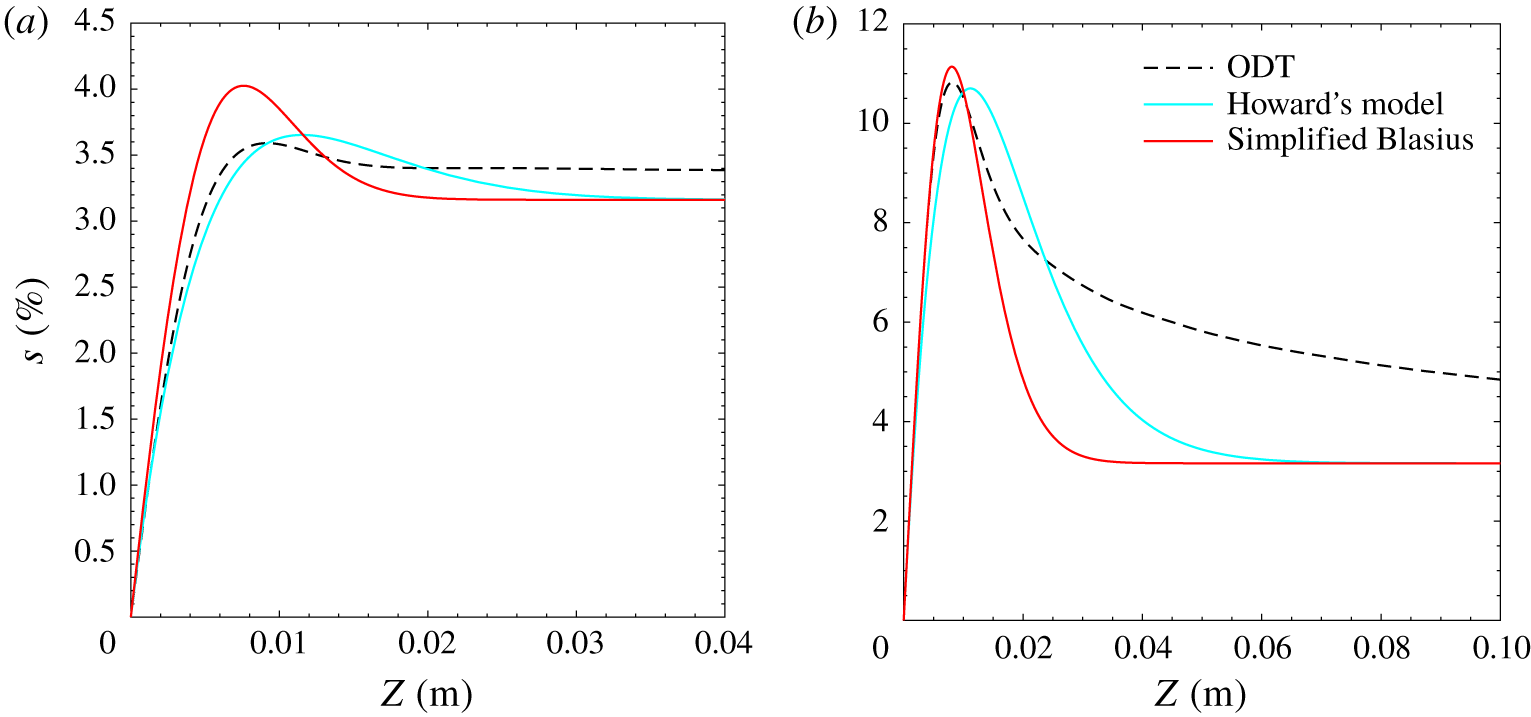
The BL mean supersaturation profile at the hot boundary: (a) an example of the s profiles for the actual diffusivity case, (b) the s profile for the case where four times higher (than actual) diffusivity of water vapour is used. Here, the black dashed curve is the simulation output, the solid red curve shows an estimation using the simplified Blasius-BL solution, and the solid cyan curve represent an estimation using Howard’s model (Howard Reference Howard1966).

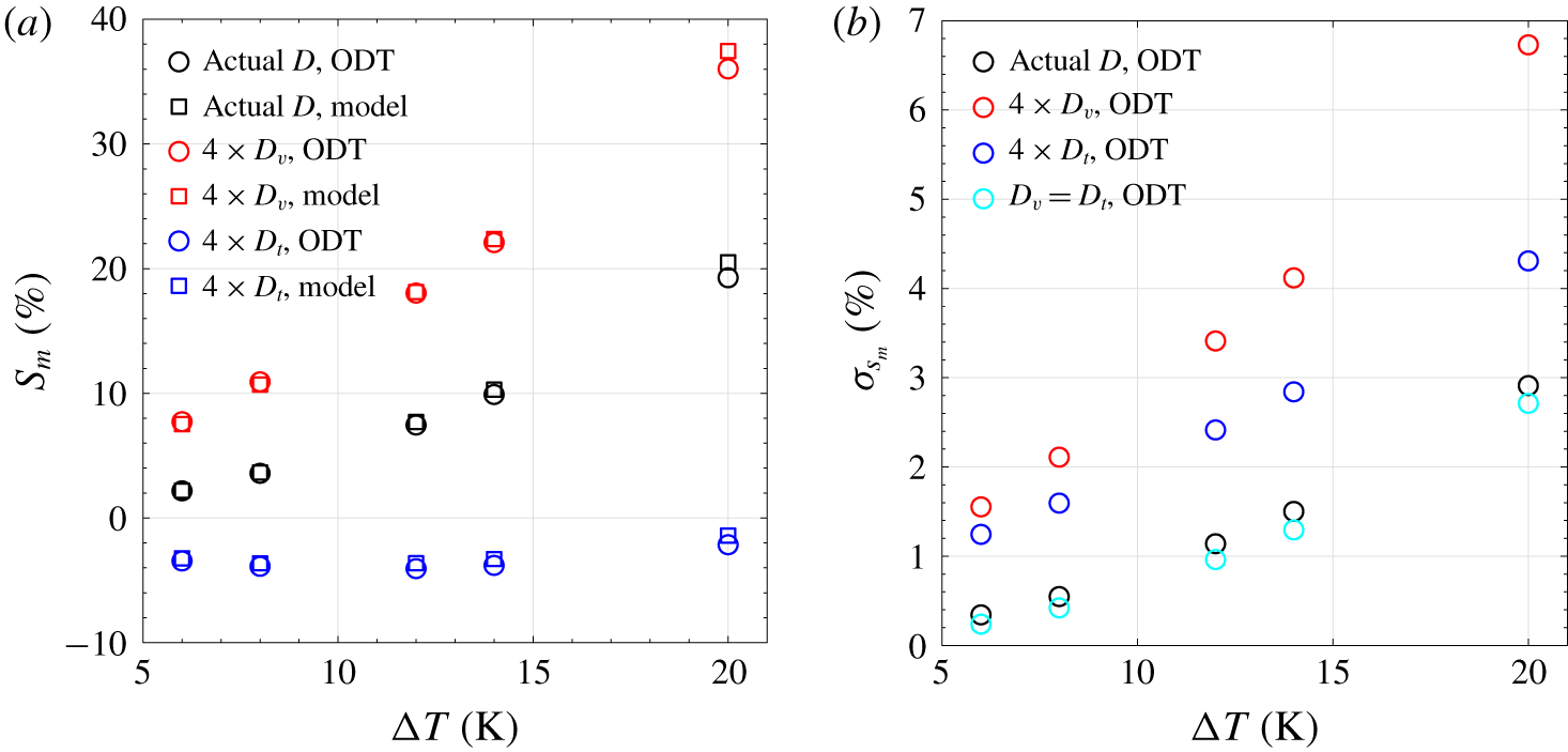
Supersaturation mean and peak standard deviation inside the BL. (a) Variation of the mean supersaturation peak with  $\unicode[STIX]{x0394}T$ and its comparison with the Howard model. (b) Maximum supersaturation standard deviation inside the BL versus applied temperature difference.

Figure 11 shows the mean supersaturation profile (near the hot boundary) obtained from the ODT simulation and its comparison with the BL solution as discussed above. Both the simulation and the estimate produce a peak of supersaturation in the BL, and the estimated magnitude of the peak is roughly consistent with the simulation. Considering the approximations used in the BL solution, it has a reasonable predictive ability. As an alternative, we also adapt the model proposed by Howard (Reference Howard1966) to predict the BL profile of supersaturation profile. As seen in figure 11, it provides a significantly improved match to the ODT. The Howard model is based on the concept of continuous eruptions of ‘thermals’ (plume) from the BL: it assumes that at some place on the hot boundary, a thermal develops during the conduction stage and because of the convective instability, it becomes detached from the boundary instantly once it reaches some critical size. A mean critical time to which a thermal develops, until which the corresponding diffusion-equation solution can be applied near the plate, is represented here as  $t^{\star }$. In turbulent convection these thermals are continuously developing and breaking off at different times and places. Therefore, the time-dependent solution of the diffusion equation needs to be averaged from 0 to
 $t^{\ast }$ and the resulted expression is (Howard Reference Howard1966)
 $$\begin{eqnarray}\bar{T}=T_{m}+\unicode[STIX]{x0394}T/2\left[(1+2\unicode[STIX]{x1D709}^{2})\text{erfc}(\unicode[STIX]{x1D709})-\frac{2\unicode[STIX]{x1D709}\text{e}^{-\unicode[STIX]{x1D709}^{2}}}{\sqrt[]{\unicode[STIX]{x03C0}}}\right].\end{eqnarray}$$
Here,  $\unicode[STIX]{x1D709}=z/(2~\sqrt[]{D_{t}t^{\ast }})$,
 $t^{\ast }=H^{2}(Ra_{\unicode[STIX]{x1D6FF}_{v}}/Ra)^{2/3}/(\unicode[STIX]{x03C0}\unicode[STIX]{x1D708})$, and
 $Ra_{\unicode[STIX]{x1D6FF}}$ is the Rayleigh number based on the critical boundary layer thickness (
 $\unicode[STIX]{x1D6FF}=\sqrt{\unicode[STIX]{x03C0}\unicode[STIX]{x1D708}t^{\ast }}$). The expression for
 $t^{\ast }$ is obtained from the definition of Rayleigh number (
 $Ra/Ra_{\unicode[STIX]{x1D6FF}}=(H/\unicode[STIX]{x1D6FF})^{3}$) and the critical boundary layer thickness (
 $\unicode[STIX]{x1D6FF}=\sqrt{\unicode[STIX]{x03C0}\unicode[STIX]{x1D708}t^{\ast }}$). Howard (Reference Howard1966) reported
 $Ra_{\unicode[STIX]{x1D6FF}}=2800$ obtained from fitting measurements made in air by Townsend (Reference Townsend1959). We use the above relation (and a similar relation for water vapour), along with
 $Ra_{\unicode[STIX]{x1D6FF}}=2800$ for obtaining the supersaturation profile shown in figure 11. The Howard model better predicts the magnitude and
 $z$-position of the peak in mean supersaturation and
 $\unicode[STIX]{x1D70E}_{s}$.
Figure 12 displays the supersaturation mean (a) and  $\unicode[STIX]{x1D70E}_{s}$ (b) peaks near the hot boundary at different
 $\unicode[STIX]{x0394}T$ and for the different diffusivity cases. Both increase monotonically with
 $\unicode[STIX]{x0394}T$. The prediction of the peak mean-
 $s$ from the Howard model is also shown in figure 12(a), and it is able to capture the trend and the magnitude remarkably well for all cases. The peak magnitude of the mean supersaturation is positive and higher for the higher water vapour diffusivity case and negative for the higher thermal diffusivity case. The fluctuations are influenced by the absolute diffusivity difference between water vapour and temperature, and is greater if one of the diffusivities is significantly larger than the other. Moreover, the peak position of supersaturation is nearly insensitive to the temperature difference in the current range of
 $Ra_{moist}$ (not shown here).
4 Summary and discussion
The problem of moist Rayleigh–Bénard convection involves buoyancy components from two driving scalars, temperature and water vapour, in a flow field, which makes it more intriguing and complex compared to its dry (single-component) convection counterpart. There is a rich variety of multi-component convection problems, ranging from double-diffusive convection (Huppert & Turner Reference Huppert and Turner1981) to particle-settling-driven convection (Burns & Meiburg Reference Burns and Meiburg2012). In this work, we consider the problem from the perspective of supersaturation, which is a nonlinear coupling of water vapour concentration and temperature fields, and is the fundamental driver of phase transformations in clouds. Cloud formation itself leads to profound changes in flow structure through latent heating, radiative transfer and particle settling, but in this work we focus solely on the supersaturation field. This view can be considered complementary to the boundary layer perspective of humidity flux budgets (Wyngaard et al. (Reference Wyngaard, Pennell, Lenschow and LeMone1978) and Mellado et al. (Reference Mellado, Puche and van Heerwaarden2017) and references therein), where covariances of temperature and absolute humidity are considered. One aspect of the problem we explicitly account for here is the difference in diffusivities of both scalars; although it is seemingly slight, we consider the extent to which it influences scalar statistics. The intent in varying the two diffusivities has been primarily to elucidate and clarify the role of differential diffusivity in determining supersaturation profiles and statistics. Beyond its purpose in exploring the dependence on differential diffusivity, there may be applications (e.g. semiconvection or cloud formation in exoplanet atmospheres) in which varying Lewis numbers play a role (Marley et al. Reference Marley, Ackerman, Cuzzi and Kitzmann2013; Zaussinger & Spruit Reference Zaussinger and Spruit2013).
Supersaturation statistics, not simply mean quantities, but properties of the fluctuations, are very important for cloud microphysical processes (Politovich & Cooper Reference Politovich and Cooper1988). The supersaturation statistics in the atmospheric boundary-layer may be dependent on surface and radiative fluxes, and other complex dynamical features of the atmospheric convection. In this article, we have investigated the supersaturation statistics in an idealized scenario of the moist R–B convection in order to gain insight into the fundamental roles of temperature and water vapour covariance, differential scalar diffusivity, and diffusion versus advection. This R–B convection perspective is also motivated by experiments performed in a turbulent moist-convection chamber, in which supersaturation variability has been proposed as contributing to important cloud properties (Chandrakar et al. Reference Chandrakar, Cantrell, Chang, Ciochetto, Niedermeier, Ovchinnikov, Shaw and Yang2016). Eventually, we aim to compare these results to experimental observations, but this will require careful development of methods capable of accurate measurement of temperature and water vapour, highly resolved in both space and time.
Central results and findings from this study may be summarized as follows:
(i) We have investigated moist R–B convection using a stochastic model (ODT), covering a range of Rayleigh number
$2.05\times 10^{8}\leqslant Ra\leqslant 2.75\times 10^{9}$. The ODT model is a numerically efficient method of exploring advection and diffusion within turbulent convection (Wunsch & Kerstein Reference Wunsch and Kerstein2005). To explore the role of relative diffusivity, four different combinations of scalar diffusivities for temperature and water vapour have been used. As a primary check, profiles of mean and standard deviation of both scalars are consistent with profiles one would expect in R–B convection.(ii) A simplistic scaling for
$Nu$ and $Sh$ is developed, based on the approaches of Malkus (Reference Malkus1954) and Howard (Reference Howard1963). The scalings and simulation results are generally self-consistent, and are in line with previous findings.(iii) In the bulk fluid,
$\unicode[STIX]{x1D70E}_{T}^{\ast }$ and $\unicode[STIX]{x1D70E}_{qv}^{\ast }$ both follow a $Ra_{moist}^{-1/6}$ scaling relation. Moreover, the magnitude of scalar fluctuations increases with an increase in the respective scalar diffusivity, as predicted from the scaling relations. An increase in thermal diffusivity decreases water vapour fluctuations, which is also consistent with derived scaling. Derivation of the scaling relations are based on the argument presented in Castaing et al. (Reference Castaing, Gunaratne, Heslot, Kadanoff, Libchaber, Thomae, Wu, Zaleski and Zanetti1989) for the single-component convection case.(iv) The correlation of both scalars is very close to 1 for a small difference in scalar diffusivities, and it decreases slightly with an increase in relative diffusivity and
$Ra_{moist}$. It also decreases further towards boundaries.(v) In a mixing diagram (
$e_{v}-T$ coordinate), data points obtained from the centre of the domain shows deviations from the idealized mixing scenario for cases with relatively different water vapour and thermal diffusivities. The scatter of data points within the space ($e_{v}-T$) is greater for the scalar with higher diffusivity. This inclination of data points corresponding to the mixing line signifies higher supersaturation fluctuations compared to the idealized mixing case.(vi) Vertical profiles of supersaturation mean and standard deviation both are nearly flat in the bulk fluid for cases with low diffusivity difference. Additionally, the mean value is close to the prediction from the ideal mixing diagram. In contrast, for cases with higher diffusivity difference, the mean profile develops a more pronounced slope and its sign flips depending on
$D_{v}>D_{t}$ or $D_{v}<D_{t}$. The $\unicode[STIX]{x1D70E}_{s}$ profile resembles the shape of both scalars and its magnitude scales with relative diffusivity difference.(vii) The p.d.f. of supersaturation become broader with an increase in absolute value of the diffusivity difference. Also, the p.d.f. is slightly negatively skewed for cases with a low diffusivity difference, unlike the
$T$ and $q_{v}$ p.d.f.s. Moreover, we have developed a scaling relation for supersaturation variance in the bulk fluid. It suggests an increase in supersaturation variance as $Ra_{moist}^{5/3}$, likewise, a relationship with $Pr$ and $Sc$. The supersaturation sampled from the centre of the domain approximately agrees with the scaling. Furthermore, the analysis of numerical output shows contributions to the supersaturation variance from both scalar variance and covariance. It indicates that all terms are equally important, although the covariance contribution can be simplified as a function of individual scalar variances since the correlation efficiency is nearly 100 %. However, this correlation efficiency might be significantly lower in atmospheric clouds (e.g. 0.24–0.34 in cumulus cloud (Siebert & Shaw Reference Siebert and Shaw2017)) due to additional relative fluxes of water vapour and heat as a result of entrainment and condensation. This certainly is a topic for further investigation.(viii) Finally, the supersaturation profile within the boundary layer has been investigated. It develops opposite-sign peaks near the two boundaries for a non-zero diffusivity difference. These peaks flip sign depending on the condition
$D_{v}>D_{t}$ or $D_{v}<D_{t}$. Additionally, supersaturation profiles in the BL obtained using scalar profiles from Prandtl–Blasius–Pohlhausen solution (for a low $Pr/Sc$ case) and from Howard’s model, both resemble the shape reasonably well. Howard’s model predicts the shape, as well as the peak magnitude and location extremely well.


The first four numbered points of this section describe the relatively modest departures of Rayeigh–Bénard convection when water vapour is included as an additional scalar. The main contribution of the current work has been to explore the supersaturation mean and fluctuation characteristics in turbulent convection, with the most significant results summarized in the last four numbered points above. These results indicate that the nonlinear coupling between both species through saturation equation and relative diffusivities of scalars influences the supersaturation statistics in an interesting way. One could extend this study further to include the effects of phase changes and accompanying latent heat release, and momentum coupling between the fluid and the condensed water, which will depend on the particle size distribution. It is also of interest to consider implications for scaling the model up to the properties that would exist for a full convective layer in the atmosphere (e.g. atmospheric boundary layer). The variance of supersaturation fluctuations in the bulk follows a  $Ra^{5/3}~H^{-6}\propto \unicode[STIX]{x0394}T^{5/3}~H^{-1}$ relation (cf. equations (3.12) and (3.13)). Thus, supersaturation variance would be expected to decrease with layer depth for a constant imposed temperature difference. Other factors such as entrainment and phase-changes would enhance the supersaturation fluctuations relative to this idealized condition, however, and this is of interest for further exploration.
The insight into the behaviour of supersaturation fluctuations in the idealized scenario considered in this study could have implications for subgrid-scale representation of fluctuations relevant to cloud droplet growth (e.g. Chandrakar et al. Reference Chandrakar, Cantrell, Chang, Ciochetto, Niedermeier, Ovchinnikov, Shaw and Yang2016). Already, the two-scalar concept has been used in representation of cloudiness in computational models of the atmosphere by combining assumed probability density functions with higher-order turbulence closure (HOC). Higher-order turbulence closure uses the equations that govern selected moments of the subgrid scale variables. For example, Sommeria & Deardorff (Reference Sommeria and Deardorff1977) and Mellor (Reference Mellor1977) independently connected the concept of assumed probability density functions with HOC. They proposed that within the grid cells of a LES, the liquid water potential temperature  $\unicode[STIX]{x1D703}_{l}$ and total water mixing ratio (vapour plus cloud droplets)
 $q_{t}$, could be assumed to have a joint Gaussian distribution. They further showed how this assumption can be used to diagnose the fractional cloudiness from the means, variances and covariance of
 $\unicode[STIX]{x1D703}_{l}$ and
 $q_{t}$. Their idea was that these moments could be determined by HOC, then used to determine the parameters of the assumed joint Gaussian for each grid cell of a model. The joint distribution could then be used to diagnose the fractional cloudiness, which in turn affects the buoyancy flux, microphysical process rates, and radiative fluxes. Cloud is assumed to exist when
 $q_{t}$ exceeds the saturation mixing ratio of water vapour,
 $q_{v}^{\ast }$ and the cloud water mixing ratio is found as
 $q_{t}-q_{v}^{\ast }$ integrated over the joint probability density function. The approach has been further generalized (Randall Reference Randall1987; Golaz et al. Reference Golaz, Larson and Cotton2002a; Golaz, Larson & Cotton Reference Golaz, Larson and Cotton2002b) and has been widely adopted. The work presented here provides additional insight, by illustrating the role of scalar diffusivity, and by providing scaling relations for boundary layer and bulk supersaturation profiles and fluctuations. A next step is to make direct comparison with laboratory measurements, as well as extending to atmospherically relevant scales.
Acknowledgements
This work was supported by National Science Foundation Grant AGS-1754244 and by the NASA Earth and Space Science Fellowship Program Grant 80NSSC17K0449.