1 Introduction
Modern microfluidic devices have revolutionized experimental study of the transport and fluid dynamics of biological cells (Dahl et al.
Reference Dahl, Lin, Muller and Kumar2015). The motion of single cells through a tight constriction has been of central interest, e.g. for understanding the hemodynamics of the microcirculation (Goldsmith & Skalak Reference Goldsmith and Skalak1975; Secomb et al.
Reference Secomb, Skalak, Oozkaya and Gross1986; Pries, Neuhaus & Gaehtgens Reference Pries, Neuhaus and Gaehtgens1992), characterizing cancer cell mechanics (Byun et al.
Reference Byun, Son, Amodei, Cermak, Shaw, Kang, Hecht, Winslow, Jacks, Mallick and Manalis2013) or developing biocompatible drug delivery carriers through ‘cell squeezing’ (Sharei et al.
Reference Sharei, Zoldan, Adamo, Sim, Cho, Jackson, Mao, Schneider, Han, Lytton-Jean, Basto, Jhunjhunwala, Lee, Heller, Kang, Hartoularos, Kim, Anderson, Langer and Jensen2013). The main attraction of microfluidic devices is the relative ease with which they may be fabricated (e.g. via soft lithography), the exquisite control over the device geometry and the small volume of fluid sample required for experimentation (Xia & Whitesides Reference Xia and Whitesides1998). Consequently, many experiments may be conducted simultaneously at relatively low cost. Moreover, at length scales of the order of
 $10{-}100~\unicode[STIX]{x03BC}\text{m}$
, inertial forces are often negligible and hence microfluidic fluid flow typically is in the Stokes regime (Squires & Quake Reference Squires and Quake2005). Useful corollaries of Stokes flow (linearity, reciprocity and temporal invariance) facilitate analysis and prediction of microfluidic device operation by hydrodynamicists.
The hydrodynamics of freely suspended particles (rigid or soft particles, droplets and biological cells) driven by a pressure gradient through a conduit is quantified by two figures of merit. The first is the translational velocity
 $U$
of a particle relative to the mean velocity
 $V$
of the suspending fluid flow. (The latter quantity
 $V$
is not to be confused with the velocity of the undisturbed flow. Both
 $U$
and
 $V$
must be measured simultaneously as the particle flows through the conduit via a controlled pressure gradient.) The relative velocity
 $U/V$
quantifies the mobility of the particle through the conduit, and is typically bounded (from above) by the maximum velocity in the channel. That is to say, the average velocity of a freely suspended particle – one free of influence of external body forces – cannot exceed the maximum velocity in the channel. For a Poiseuille flow through a circular tube, this upper bound is set by
 $2V$
. The particle translational velocity
 $U$
is relatively easy to measure by tracking its position in time (Savin, Bandi & Mahadevan Reference Savin, Bandi and Mahadevan2016). The mean fluid velocity
 $V$
must be simultaneously measured, e.g. by measuring the flow rate through a ‘reference channel’ driven by the same pressure gradient as a ‘test channel’ containing the particle. Thus, the relative velocity
 $U/V$
is a relatively simple metric for quantifying the hindered mobility of particles due to channel confinement.
The second hydrodynamic figure of merit is the extra pressure drop
 $\unicode[STIX]{x0394}p^{+}$
created by the presence of a suspended particle (Brenner Reference Brenner1970, Reference Brenner1971). The extra pressure drop is an intrinsic measure of particle dissipation in channel flow, akin to the intrinsic (or per particle) viscosity measured in a shear-flow experiment of a dilute suspension. Fluid flow in a conduit creates dissipation on the conduit walls, which in turn must be balanced by a driving pressure force. In the absence of suspended particles, the pressure drop
 $\unicode[STIX]{x0394}p^{\circ }$
required to drive a Newtonian fluid through a duct of constant cross-section at a (steady) flow rate
 $Q$
is given by Poiseuille’s law,
 $$\begin{eqnarray}\unicode[STIX]{x0394}p^{\circ }=L_{c}K_{hyd}Q,\end{eqnarray}$$
where
 $L_{c}$
is the channel length and
 $K_{hyd}$
is a hydraulic resistance coefficient that depends only on the shear viscosity
 $\unicode[STIX]{x1D707}$
of the fluid and the geometry of the duct. For cylindrical conduits, the hydraulic resistance is maximized when the cross-section is circular. For example, letting
 $R$
be the channel hydraulic radius and
 $\unicode[STIX]{x1D707}$
the suspending fluid viscosity,
 $R^{4}K_{hyd}/\unicode[STIX]{x1D707}=8/\unicode[STIX]{x03C0}\simeq 2.55$
for a circular tube, 1.78 for a square duct and
 $20/(9\sqrt{3})\simeq 1.28$
for an equilateral triangular duct (White Reference White1991). The flow rate
 $Q$
is related to the mean fluid velocity
 $V$
by
 $$\begin{eqnarray}Q=A_{\times }V,\end{eqnarray}$$
where
 $A_{\times }$
is the area of a cross-section (e.g.
 $A_{\times }/R^{2}=\unicode[STIX]{x03C0}\simeq 3.14$
for a circular tube,
 $4$
for a square duct and
 $3\sqrt{3}\simeq 5.20$
for a triangular duct). Introducing particles into the fluid creates a disturbance velocity field and hence the total pressure drop
 $\unicode[STIX]{x0394}p=\unicode[STIX]{x0394}p^{\circ }+\unicode[STIX]{x0394}p^{+}$
required to push the particle suspension through the duct at the same flow rate
 $Q$
is altered (for most systems,
 $\unicode[STIX]{x0394}p>\unicode[STIX]{x0394}p^{\circ }$
). The dimensionless extra pressure drop
 $\unicode[STIX]{x0394}p^{+}R/(\unicode[STIX]{x1D707}V)$
can be directly related to the apparent intrinsic viscosity of the particle suspension at known concentration
 $c$
, and thus gives a measure of the suspension rheology (Tözeren & Skalak Reference Tözeren and Skalak1978; Barakat Reference Barakat2018).
Aside from the suspension concentration, the primary control parameter that determines the relative velocity
 $U/V$
and dimensionless extra pressure drop
 $\unicode[STIX]{x0394}p^{+}R/(\unicode[STIX]{x1D707}V)$
is the ratio between the characteristic radius of the particle
 $R_{0}$
and the hydraulic radius of the channel
 $R$
,
 $\unicode[STIX]{x1D706}=R_{0}/R$
. Biological cells can deform under the action of hydrodynamic stresses, and so the dimensionless groups
 $U/V$
and
 $\unicode[STIX]{x0394}p^{+}R/(\unicode[STIX]{x1D707}V)$
for cellular suspensions are also nonlinearly coupled to cell shape configurations. Early studies of cellular flow through narrow channels neglected this dependence by focusing on ‘rigid-particle models’, mostly in circular-tube geometries (Brenner & Happel Reference Brenner and Happel1958; Goldsmith & Mason Reference Goldsmith and Mason1962; Lighthill Reference Lighthill1968; Wang & Skalak Reference Wang and Skalak1969; Brenner Reference Brenner1970; Chen & Skalak Reference Chen and Skalak1970; Hochmuth & Sutera Reference Hochmuth and Sutera1970). In the Stokes-flow regime, the equations governing the flow of rigid particles in bounded domains are linear, provided that their configurations in space and time are known. In order to make analytical progress in theoretical calculations, often the particle configurations are simplified, e.g. by assuming diluteness or some well-defined structure to the suspension. The main results from studies of rigid particles flowing through circular tubes show that, for particle dimensions
 $R_{0}$
of the order of the tube radius
 $R$
, the relative velocity
 $U/V$
is in excess of unity by an amount proportional to the flow area through which fluid may bypass the particle. The dimensionless extra pressure drop
 $\unicode[STIX]{x0394}p^{+}R/(\unicode[STIX]{x1D707}V)$
typically diverges in proportion to some power of the reciprocal gap thickness, say
 $(R-R_{0})^{-1}$
. The strength of this singularity depends on the particle surface curvature at the point of contact, e.g. the singularity is of
 $O[(R-R_{0})^{-1/2}]$
for spherical particles and
 $O[(R-R_{0})^{-1}]$
for cylindrical particles whose axis is coincident with the channel axis.
Later theoretical studies of cellular flow through conduits incorporated intrinsic cellular mechanics, using white blood cells (Tözeren & Skalak Reference Tözeren and Skalak1978), red blood cells (Secomb et al. Reference Secomb, Skalak, Oozkaya and Gross1986; Halpern & Secomb Reference Halpern and Secomb1989) and vesicles (Bruinsma Reference Bruinsma1996; Trozzo et al. Reference Trozzo, Boedec, Leonetti and Jaeger2015; Barakat & Shaqfeh Reference Barakat and Shaqfeh2018a ,Reference Barakat and Shaqfeh b ) as model systems. The material properties of the cell thus become parameters in the flow system. The most basic cellular models typically fall into one of three categories:
(i) The entire cell volume is treated as an elastic solid with bulk elastic moduli. This is a common model for white blood cells.
(ii) The membrane is treated as a two-dimensional solid, with elastic properties akin to that of a thin shell. The principal deformation modes include in-plane shear and dilatation (with surface elastic moduli
 $E_{S}$
and
$E_{D}$
, respectively, with units of force
$\div$
distance) and out-of-plane bending (
$E_{B}$
has units of force
$\times$
distance). Typically, the dilatational modulus
$E_{D}$
is very large, of the order of
$200~\text{mN}~\text{m}^{-1}$
(Evans & Needham Reference Evans and Needham1987), so a common approximation is to assume that the membrane is surface-area incompressible. This is the common type of model used for red blood cells (Skalak et al.
Reference Skalak, Tozeren, Zarda and Chien1973).
(iii) The membrane is treated as a two-dimensional incompressible fluid with surface shear viscosity
$\unicode[STIX]{x1D702}_{s}$
(units of force
$\times$
time
$\div$
distance). Out-of-plane deformation is governed by a bending-elastic modulus
$E_{B}$
. The bending modulus of giant, unilamellar vesicles is approximately
$10^{-13}~\unicode[STIX]{x03BC}\text{N}~\text{m}$
(Evans & Needham Reference Evans and Needham1987). Typically, the surface shear viscosity
$\unicode[STIX]{x1D702}_{s}$
of membranes is small, of the order of
$10^{-3}{-}10^{-2}~\unicode[STIX]{x03BC}\text{N}~\text{s}~\text{m}^{-1}$
(Evans & Needham Reference Evans and Needham1987; Evans & Yeung Reference Evans and Yeung1994). Vesicles, which lack the spectrin-actin cortex and hence the in-plane shear elasticity of red blood cells, are typically modelled in this way (Helfrich Reference Helfrich1973).



The importance of accounting for intrinsic cellular mechanics is twofold. Firstly, cellular deformation influences the cell shape and hence the hydrodynamics. This effect is inherently nonlinear and can lead to ‘non-Newtonian behaviour’, meaning that the extra pressure drop
 $\unicode[STIX]{x0394}p^{+}$
no longer scales linearly with the imposed mean velocity
 $V$
. Secondly, membrane flow can qualitatively affect the flow in the suspending fluid. For circularly symmetric systems, cells enclosed by incompressible membranes have uniform surface velocity; hence, they behave much like rigid particles in circular Poiseuille flow.
All of the studies mentioned above, both for rigid particles and more realistic ‘model cells’, have focused on flow through circular tubes. One of the main motivations for studying this geometry originates in the study of blood flow through the circulatory system. In fact, Poiseuille’s original study of blood flow in the microcirculation is what led to his eponymous law (Sutera & Skalak Reference Sutera and Skalak1993). From a mathematical point of view, the additional simplicity gained by considering a conduit whose cross-section possesses circular symmetry also facilitates analysis. However, fluid experimentation nowadays makes use of microfluidic devices fabricated using soft lithography. The resulting channels are either square or rectangular in cross-section, not circular. Unfortunately, theoretical studies of particulate flow through non-circular conduits are relatively sparse (Tullock, Phan Thien & Graham Reference Tullock, Phan and Graham1992). (The closely analogous ‘plane-Poiseuille flow’ is not included in this group, since the areal cross-section is not well defined and thus the quantities
 $U/V$
and
 $\unicode[STIX]{x0394}p^{+}R/(\unicode[STIX]{x1D707}V)$
cease to have meaning.) Far from being a trivial change, it is expected that the duct cross-section has a qualitative effect on the hydrodynamics due to the broken symmetry about the channel axis. Two of the authors of the present work have previously compared the relative velocity
 $U/V$
of wax particles, vesicles and cancer cells travelling through square ducts (Ahmmed et al.
Reference Ahmmed, Suteria, Garbin and Vanapalli2018). In this work, it was shown that the relative velocity of cancer cells is higher than that of solid particles but lower than that of vesicles for fixed radius ratio
 $\unicode[STIX]{x1D706}=R_{0}/R$
, presumably due to differences in surface mobility. The marked differences observed between these three systems, in addition to qualitative deviations from the circular-tube geometry, motivates additional experimentation as well as a theoretical complement.
The purpose of the present work is to investigate the hydrodynamics of a model cell – a vesicle – in conduit flow with a non-circular cross-section. The specific case considered in this work is that of square cross-section, which has particular relevance to microfluidics. The theoretical problem of calculating the relative velocity
 $U/V$
and dimensionless extra pressure drop
 $\unicode[STIX]{x0394}p^{+}R/(\unicode[STIX]{x1D707}V)$
for a vesicle freely suspended in channel flow is solved herein using boundary element simulations and lubrication theory. Bending elasticity and membrane shear viscosity are neglected in the model, so that the only characteristic feature of the vesicles is that they have incompressible surfaces. Experimental measurements are performed using a microfluidic manometer, previously used to study droplets, wax particles, vesicles and cancer cells (Vanapalli et al.
Reference Vanapalli, Banpurkar, van den Ende, Duits and Mugele2009; Khan & Vanapalli Reference Khan and Vanapalli2013; Khan et al.
Reference Khan, Kamyabi, Hussain and Vanapalli2017). Excellent agreement between theory and experiment is achieved. It is shown that vesicular hydrodynamics in the square cross-section is qualitatively different than that in a circular cross-section, previously investigated by two of the authors (Barakat & Shaqfeh Reference Barakat and Shaqfeh2018a
,Reference Barakat and Shaqfeh
b
).
This paper is organized as follows. In § 2, the governing equations of hydrodynamics are posed in conjunction with the equations of mechanical equilibrium for the vesicle membrane. The boundary element method (BEM) used in this work is introduced in § 3. A lubrication theory is developed in § 4. The experimental methods are presented in § 5. A discussion of the results, including comparison between theory and experiment, is presented in § 6. Concluding remarks are given in § 7.
2 Theoretical formulation
2.1 Governing equations
A schematic of the problem is shown in figure 1 with Cartesian axes
 $(x,y,z)=(x_{1},x_{2},x_{3})$
. A vesicle with volume
 $\unicode[STIX]{x1D6FA}_{0}$
and surface area
 $A_{0}$
enters a square duct and flows until it reaches some fully developed configuration (independent of end effects). The hydraulic radius of the duct is
 $R$
, defined as twice the ratio of the flow area to the wetted perimeter of the duct. In the creeping-flow regime, the fluid velocity
 $\boldsymbol{u}$
and stress
 $\unicode[STIX]{x1D64E}$
satisfy the Stokes equations (written below in Einstein notation),
 $$\begin{eqnarray}\displaystyle & \displaystyle \left\{\begin{array}{@{}l@{}}\displaystyle \frac{\unicode[STIX]{x2202}u_{j}}{\unicode[STIX]{x2202}x_{j}}=0\quad \\ \displaystyle \frac{\unicode[STIX]{x2202}\unicode[STIX]{x1D61A}_{ij}}{\unicode[STIX]{x2202}x_{j}}=-\frac{\unicode[STIX]{x2202}p}{\unicode[STIX]{x2202}x_{i}}+\unicode[STIX]{x1D707}\unicode[STIX]{x1D6FB}^{2}u_{i}=0\quad \end{array}\right.\quad \text{in the suspending fluid}, & \displaystyle\end{eqnarray}$$
 $$\begin{eqnarray}\displaystyle & \displaystyle \left\{\begin{array}{@{}l@{}}\displaystyle \frac{\unicode[STIX]{x2202}u_{j}}{\unicode[STIX]{x2202}x_{j}}=0\quad \\ \displaystyle \frac{\unicode[STIX]{x2202}\unicode[STIX]{x1D61A}_{ij}}{\unicode[STIX]{x2202}x_{j}}=-\frac{\unicode[STIX]{x2202}p}{\unicode[STIX]{x2202}x_{i}}+\hat{\unicode[STIX]{x1D707}}\unicode[STIX]{x1D6FB}^{2}u_{i}=0\quad \end{array}\right.\quad \text{within the vesicle}, & \displaystyle\end{eqnarray}$$
 $\unicode[STIX]{x1D707}$
is the exterior fluid viscosity,
 $\hat{\unicode[STIX]{x1D707}}$
is the interior fluid viscosity and
 $p$
is the fluid pressure (a Lagrange field that enforces volume incompressibility). The vesicle is forced into motion by a mean velocity
 $V$
, where
 $$\begin{eqnarray}VA_{\times }=\int _{\mathscr{S}_{\times }}u_{1}\,\text{d}S\quad \text{as }x_{1}\rightarrow \pm \infty .\end{eqnarray}$$
Here,
 $\mathscr{S}_{\times }$
denotes a cross-sectional surface in the channel with surface area
 $A_{\times }$
. On the channel wall, the velocity
 $\boldsymbol{u}$
is subject to the no-slip condition,
 $$\begin{eqnarray}u_{i}=0\quad \text{on the channel wall}.\end{eqnarray}$$
The vesicle membrane is treated as an internally fluid, incompressible surface with unit normal
 $\boldsymbol{n}$
. Surface-area incompressibility implies that
 $$\begin{eqnarray}\unicode[STIX]{x1D617}_{ij}\frac{\unicode[STIX]{x2202}u_{i}}{\unicode[STIX]{x2202}x_{j}}=0\quad \text{on the vesicle membrane},\end{eqnarray}$$
where
 $\unicode[STIX]{x1D64B}=\unicode[STIX]{x1D644}-\boldsymbol{n}\boldsymbol{n}$
is the surface projection tensor. The velocity
 $\boldsymbol{u}$
is continuous across the membrane surface, whereas the stress
 $\unicode[STIX]{x1D64E}$
undergoes a jump. Neglecting bending elasticity, the membrane boundary conditions read
 $$\begin{eqnarray}\left\{\begin{array}{@{}l@{}}\displaystyle \unicode[STIX]{x27E6}u_{i}\unicode[STIX]{x27E7}=0\quad \\ \displaystyle n_{i}\unicode[STIX]{x27E6}\,f_{i}\unicode[STIX]{x27E7}=-2H\unicode[STIX]{x1D70F}\quad \\ \displaystyle P_{ij}\unicode[STIX]{x27E6}\,f_{j}\unicode[STIX]{x27E7}=-P_{ij}\frac{\unicode[STIX]{x2202}\unicode[STIX]{x1D70F}}{\unicode[STIX]{x2202}x_{j}}\quad \end{array}\right.\quad \text{on the vesicle membrane},\end{eqnarray}$$
where
 $\unicode[STIX]{x27E6}\,\cdot \,\unicode[STIX]{x27E7}$
is the ‘jump’ operator,
 $H=-[(\unicode[STIX]{x1D64B}\boldsymbol{\cdot }\unicode[STIX]{x1D735})\boldsymbol{\cdot }\boldsymbol{n}]/2$
is the mean curvature,
 $\boldsymbol{f}=\unicode[STIX]{x1D64E}\boldsymbol{\cdot }\boldsymbol{n}$
is the fluid traction and
 $\unicode[STIX]{x1D70F}$
is the membrane tension (a Lagrange field that enforces surface-area incompressibility). The justification for neglecting bending elasticity in (2.5) is provided at the end of this section.
Schematic of a vesicle driven by a pressure gradient through a square duct, drawn in a reference frame translating with the vesicle velocity
 $U$
.

Since the vesicle membrane is a free surface, the kinematic condition further requires that it translate with the local fluid velocity,
 $$\begin{eqnarray}\frac{\text{D}x_{si}}{\text{D}t}=\frac{\unicode[STIX]{x2202}x_{si}}{\unicode[STIX]{x2202}t}+u_{j}\frac{\unicode[STIX]{x2202}x_{si}}{\unicode[STIX]{x2202}x_{j}}=u_{i}\quad \text{on the vesicle membrane},\end{eqnarray}$$
where
 $\text{D}/\text{D}t$
is the material derivative and
 $\boldsymbol{x}_{s}$
denotes the position of a point on the membrane. The unit normal
 $\boldsymbol{n}$
can be related to
 $\boldsymbol{x}_{s}$
via standard relations from differential geometry (Kreyszig Reference Kreyszig1959).
Although the governing Stokes equations are steady, the boundary-value problem is time dependent through the kinematic condition (2.6). Thus, the system is evolved starting from some initial configuration for the vesicle shape. At the initial time point, the total vesicle volume
 $\unicode[STIX]{x1D6FA}_{0}$
and surface area
 $A_{0}$
are prescribed:
 $$\begin{eqnarray}\text{at }t=0:\int _{\mathscr{V}_{s}}\text{d}^{3}\boldsymbol{x}=\unicode[STIX]{x1D6FA}_{0},\quad \int _{\mathscr{S}_{s}}\,\text{d}S=A_{0},\end{eqnarray}$$
where
 $\mathscr{V}_{s}$
is the region occupied by the vesicle and
 $\mathscr{S}_{s}=\unicode[STIX]{x2202}\mathscr{V}_{s}$
. Thus,
 $\unicode[STIX]{x1D6FA}_{0}$
and
 $A_{0}$
take the role of parameters in the initial boundary-value problem. The conditions of surface-area and volume incompressibility require that
 $\unicode[STIX]{x1D6FA}_{0}$
and
 $A_{0}$
be time-invariant in the Lagrangian sense,
 $$\begin{eqnarray}\frac{\text{D}\unicode[STIX]{x1D6FA}_{0}}{\text{D}t}=0,\quad \frac{\text{D}A_{0}}{\text{D}t}=0.\end{eqnarray}$$
2.2 Vesicle velocity and extra pressure drop
The translational velocity of the vesicle is defined as the volume average of the internal velocity field,
 $$\begin{eqnarray}U_{i}=\frac{1}{\unicode[STIX]{x1D6FA}_{0}}\int _{\mathscr{V}_{s}}u_{i}\,\text{d}^{3}\boldsymbol{x}=\frac{1}{\unicode[STIX]{x1D6FA}_{0}}\int _{\mathscr{S}_{s}}x_{i}u_{j}n_{j}\,\text{d}S,\end{eqnarray}$$
which follows from the fact that the velocity is solenoidal. The rotational velocity of the vesicle is not of interest here. The axial component of
 $\boldsymbol{U}$
is denoted by
 $U$
, and
 $U/V$
denotes the relative velocity of the vesicle with respect to the mean flow.
The extra pressure drop
 $\unicode[STIX]{x0394}p^{+}$
is obtained by requiring the vesicle to be force-free. Applying a force balance to a control volume containing the suspending fluid, bounded externally by the duct walls and internally by the vesicle surface, results in the following condition,
 $$\begin{eqnarray}\unicode[STIX]{x0394}pA_{\times }\unicode[STIX]{x1D6FF}_{1i}=-\!\int _{\mathscr{S}_{w}}f_{i}\,\text{d}S,\end{eqnarray}$$
where
 $\mathscr{S}_{w}$
is the wall surface and
 $\unicode[STIX]{x0394}p$
is the pressure drop over a distance
 $L_{c}$
(the length of the channel). Taking the formal limit as
 $L_{c}\rightarrow \infty$
results in a diverging pressure drop. A bounded quantity may be obtained by first subtracting out the Poiseuille-flow contribution and taking the limit thereafter:
 $$\begin{eqnarray}\unicode[STIX]{x0394}p^{+}=\lim _{L_{c}\rightarrow \infty }(\unicode[STIX]{x0394}p-\unicode[STIX]{x0394}p^{\circ })=\lim _{L_{c}\rightarrow \infty }(\unicode[STIX]{x0394}p-L_{c}A_{\times }K_{hyd}V),\end{eqnarray}$$
which follows from (1.1)–(1.2). The dimensionless extra pressure drop
 $\unicode[STIX]{x0394}p^{+}R/(\unicode[STIX]{x1D707}V)$
can be directly related to the apparent intrinsic viscosity of the vesicle–fluid system (Barakat Reference Barakat2018).
2.3 Scalings and dimensionless groups
To recast the problem in dimensionless form, all variables with units of distance are scaled by the channel hydraulic radius
 $R$
, fluid velocity
 $\boldsymbol{u}$
by the mean velocity
 $V$
, fluid pressure
 $p$
by
 $\unicode[STIX]{x1D707}V/R$
and membrane tension
 $\unicode[STIX]{x1D70F}$
by
 $\unicode[STIX]{x1D707}V$
. The relevant dimensionless groups are
 $$\begin{eqnarray}\left.\begin{array}{@{}c@{}}\displaystyle \unicode[STIX]{x1D705}=\frac{\hat{\unicode[STIX]{x1D707}}}{\unicode[STIX]{x1D707}}\quad \text{(the viscosity ratio)},\\ \displaystyle \unicode[STIX]{x1D706}=\frac{R_{0}}{R}\quad \text{(the radius ratio)},\\ \displaystyle \unicode[STIX]{x1D710}=\frac{\unicode[STIX]{x1D6FA}_{0}}{{\textstyle \frac{4}{3}}\unicode[STIX]{x03C0}R_{0}^{3}}\quad \text{(the reduced volume)}.\end{array}\right\}\end{eqnarray}$$
Here,
 $R_{0}=\sqrt{A_{0}/(4\unicode[STIX]{x03C0})}$
is the effective vesicle radius based on surface area. The physical significance of these dimensionless groups is easily interpreted. The viscosity ratio
 $\unicode[STIX]{x1D705}$
is a measure of the relative dissipation between the interior and exterior fluids. The reduced volume
 $\unicode[STIX]{x1D710}$
varies between 0 and 1 and gauges the degree of sphericity of the vesicle shape (a reduced volume of unity corresponds to a perfectly spherical vesicle). Since the vesicle volume
 $\unicode[STIX]{x1D6FA}_{0}$
and surface area
 $A_{0}$
are assumed to be fixed quantities,
 $\unicode[STIX]{x1D710}$
is a geometric parameter that is unaffected by flow and membrane deformation. The radius ratio
 $\unicode[STIX]{x1D706}$
, which was introduced previously, relates the characteristic dimension of the vesicle to the characteristic dimension of the channel cross-section. Thus,
 $\unicode[STIX]{x1D706}$
is a measure for flow confinement: as
 $\unicode[STIX]{x1D706}$
increases, the vesicle’s motion is more significantly hindered by vesicle–wall interactions.
Under typical experimental conditions, using water as the typical working fluid (with some combination of dissolved electrolytes),
 $\unicode[STIX]{x1D707}\approx \hat{\unicode[STIX]{x1D707}}\approx 1~\text{mN}~\text{s}~\text{m}^{-2}$
and one may reasonably assume that
 $\unicode[STIX]{x1D705}\approx 1$
. The square microchannels considered in this work have dimensions
 $R\simeq 12~\unicode[STIX]{x03BC}\text{m}$
. Giant, unilamellar vesicles span a distribution of length scales ranging from
 $1{-}100~\unicode[STIX]{x03BC}\text{m}$
. Thus, the radius ratio
 $\unicode[STIX]{x1D706}$
can take on a range of values. When prepared using electroformation, these vesicles are typically spherical or nearly spherical, meaning that their reduced volume
 $\unicode[STIX]{x1D710}$
is of
 $O(1)$
. In this work, reduced volumes in the range
 $0.85\leqslant \unicode[STIX]{x1D710}\leqslant 1$
are considered.
It is apparent that no dimensionless group relating the intrinsic vesicular mechanics to the strength of flow has been introduced, and this choice requires some clarification. Namely, it is well known that vesicle membranes have intrinsic mechanical properties that can compete with hydrodynamic stresses created by fluid flow. Among them, the bending stiffness
 $E_{B}$
of the membrane is perhaps the most significant, as it directly influences the shape through the normal component of the local stress balance on the membrane. The effect of bending elasticity on vesicle motion through circular tubes was previously investigated by two of the authors, who determined that this effect is suppressed when
 $\unicode[STIX]{x1D706}$
or
 $\unicode[STIX]{x1D710}$
are large (Barakat & Shaqfeh Reference Barakat and Shaqfeh2018a
,Reference Barakat and Shaqfeh
b
). To gauge the strength of bending forces relative to viscous forces, one has to compare
 $E_{B}$
to the characteristic viscous energy scale
 $\unicode[STIX]{x1D707}VR^{2}$
. A typical bending modulus of giant, unilamellar vesicles is
 $E_{B}\simeq 10^{-13}~\unicode[STIX]{x03BC}\text{N}~\text{m}$
(Evans & Needham Reference Evans and Needham1987). Typical mean fluid velocities in the microfluidic devices presented in § 5 are
 $V=1{-}5~\text{cm}~\text{s}^{-1}$
, which gives a viscous energy scale
 $\unicode[STIX]{x1D707}VR^{2}\simeq 10^{-9}~\unicode[STIX]{x03BC}\text{N}~\text{m}$
. (One could make the argument that the vesicle radius
 $R_{0}$
is the proper length scale to use here. However, the channel hydraulic radius
 $R$
typically bounds the membrane radius of curvature, making it the more suitable choice of length scale.) Thus, the dimensionless group
 $E_{B}/(\unicode[STIX]{x1D707}VR^{2})=O(10^{-4})$
is small enough to justify the neglect of membrane bending elasticity. Exceptional circumstances can arise when the local (deviatoric) curvature of the vesicle membrane becomes large. However, these situations never arise for vesicles that are ‘sphere-like’ (
 $\unicode[STIX]{x1D710}=O(1)$
), which are the subjects of the present study.
By neglecting bending elasticity, the only intrinsic characteristic of the vesicle membrane is that it is an incompressible surface. Strictly speaking, the vesicle membrane has a measurable dilatational modulus
 $E_{D}$
, akin to that of red blood cells, and is typically approximately
 $200~\text{mN}~\text{m}^{-1}$
. The analogous viscous scale is
 $\unicode[STIX]{x1D707}V\simeq 10^{-2}~\text{mN}~\text{m}^{-1}$
, giving a ratio
 $E_{D}/(\unicode[STIX]{x1D707}V)=O(10^{4})$
. This estimate suggests that the membrane cannot stretch significantly in the flow regime of interest (Marmottant & Hilgenfeldt Reference Marmottant and Hilgenfeldt2003; Vitkova, Mader & Podgorski Reference Vitkova, Mader and Podgorski2004). It is possible that large extensional stresses can be created locally, e.g. when the separation between the vesicle membrane and the duct wall becomes small. Under such circumstances, local dilatation can change the membrane surface area. However, this change is bounded by the maximally allowed areal strain (approximately 1 %–2 %) before the membrane ruptures (Evans & Needham Reference Evans and Needham1986). Thus, it is expected that the vesicle membrane conserves surface area locally to within a reasonable degree of accuracy.
3 Boundary element method (BEM)
The initial boundary-value problem posed in the previous section is nonlinear and spatially complex in three dimensions. Hence, direct solution requires an efficient numerical method. A fully three-dimensional (3-D) simulation method to study the motion of vesicles in conduit flow has been previously reported (Barakat & Shaqfeh Reference Barakat and Shaqfeh2018a
). Although the method has been used to study vesicle flow in circular tubes, in fact it is completely generalizable to conduits of any cross-section because singularities (of a priori unknown strength) are distributed over the wall surface. Thus, the wall surface tractions
 $\boldsymbol{f}_{w}$
must be determined simultaneously with the membrane surface velocities
 $\boldsymbol{u}_{s}$
and membrane tension
 $\unicode[STIX]{x1D70F}$
.
In brief, the vesicle and channel are placed in an
 $L_{x}\times L_{y}\times L_{z}$
unit cell with periodic boundary conditions applied at the bounding surfaces. The axial length
 $L_{x}$
is chosen sufficiently large such that periodic images in the
 $x$
-direction do not interact. The Stokes equations (2.1) are reformulated as integral equations with built-in boundary conditions for the membrane surface velocity
 $\boldsymbol{u}_{s}$
and wall surface traction
 $\boldsymbol{f}_{w}$
:
 $$\begin{eqnarray}\left[\begin{array}{@{}cc@{}}\displaystyle \int _{\mathscr{S}_{s}}\unicode[STIX]{x1D608}_{ij}(\boldsymbol{x},\boldsymbol{x}_{s}) & \displaystyle \int _{\mathscr{S}_{w}}\unicode[STIX]{x1D609}_{ij}(\boldsymbol{x},\boldsymbol{x}_{s})\\ \displaystyle \int _{\mathscr{S}_{s}}\unicode[STIX]{x1D60A}_{ij}(\boldsymbol{x},\boldsymbol{x}_{w}) & \displaystyle \int _{\mathscr{S}_{w}}\unicode[STIX]{x1D60B}_{ij}(\boldsymbol{x},\boldsymbol{x}_{w})\end{array}\right]\left[\begin{array}{@{}c@{}}u_{si}(\boldsymbol{x})\\ f_{wi}(\boldsymbol{x})\end{array}\right]\,\text{d}S(\boldsymbol{x})=\left[\begin{array}{@{}c@{}}b_{j}(\boldsymbol{x}_{s})\\ b_{j}(\boldsymbol{x}_{w})\end{array}\right],\end{eqnarray}$$
where
 $$\begin{eqnarray}\left.\begin{array}{@{}c@{}}\displaystyle \unicode[STIX]{x1D608}_{ij}(\boldsymbol{x},\boldsymbol{x}_{0})=\frac{1+\unicode[STIX]{x1D705}}{2}\unicode[STIX]{x1D6FF}(\boldsymbol{x}-\boldsymbol{x}_{0})\unicode[STIX]{x1D612}_{ij}(\boldsymbol{x})-\frac{1-\unicode[STIX]{x1D705}}{8\unicode[STIX]{x03C0}}\unicode[STIX]{x1D61B}_{ijk}(\boldsymbol{x},\boldsymbol{x}_{0})n_{k}(\boldsymbol{x}),\\ \displaystyle \unicode[STIX]{x1D609}_{ij}(\boldsymbol{x},\boldsymbol{x}_{0})=\frac{1}{8\unicode[STIX]{x03C0}\unicode[STIX]{x1D707}}\unicode[STIX]{x1D60E}_{ij}(\boldsymbol{x},\boldsymbol{x}_{0}),\\ \displaystyle \unicode[STIX]{x1D60A}_{ij}(\boldsymbol{x},\boldsymbol{x}_{0})=-\frac{1-\unicode[STIX]{x1D705}}{8\unicode[STIX]{x03C0}}\unicode[STIX]{x1D61B}_{ijk}(\boldsymbol{x},\boldsymbol{x}_{0})n_{k}(\boldsymbol{x}),\\ \displaystyle \unicode[STIX]{x1D60B}_{ij}(\boldsymbol{x},\boldsymbol{x}_{0})=\frac{1}{8\unicode[STIX]{x03C0}\unicode[STIX]{x1D707}}\unicode[STIX]{x1D60E}_{ij}(\boldsymbol{x},\boldsymbol{x}_{0})\end{array}\right\}\end{eqnarray}$$
are the kernels, and
 $$\begin{eqnarray}b_{j}(\boldsymbol{x}_{0})=-\frac{1}{8\unicode[STIX]{x03C0}\unicode[STIX]{x1D707}}\int _{\mathscr{S}_{s}}f_{si}(\boldsymbol{x})\unicode[STIX]{x1D60E}_{ij}(\boldsymbol{x},\boldsymbol{x}_{0})\,\text{d}S(\boldsymbol{x})+\langle u_{j}\rangle\end{eqnarray}$$
is the source. Here,
 $\langle \boldsymbol{u}\rangle$
is the volume-averaged velocity in the computational box,
 $\boldsymbol{f}_{s}=\unicode[STIX]{x27E6}\,\boldsymbol{f}(\boldsymbol{x}\in \mathscr{S}_{s})\unicode[STIX]{x27E7}$
is the jump in surface traction across the membrane,
 $\unicode[STIX]{x1D642}$
and
 $\unicode[STIX]{x1D64F}$
are the periodic Green’s functions of Hasimoto (Reference Hasimoto1959) and
 $\unicode[STIX]{x1D646}$
is the principal-value tensor. (If the field point
 $\boldsymbol{x}_{0}$
lies on a Lyapunov smooth surface, then
 $\unicode[STIX]{x1D646}=\unicode[STIX]{x1D644}$
.)
The boundary integral equations (3.1) are solved using the collocation method (Pozrikidis Reference Pozrikidis1992). The vesicle membrane and duct wall are discretized using unstructured, triangulated meshes and the unknown density fields are approximated using piecewise linear shape functions along the boundary elements. The Green’s functions
 $\unicode[STIX]{x1D642}$
and
 $\unicode[STIX]{x1D64F}$
are evaluated on the boundaries using the smooth particle mesh Ewald (SPME) algorithm (Saintillan, Darve & Shaqfeh Reference Saintillan, Darve and Shaqfeh2005; Zhao et al.
Reference Zhao, Isfahani, Olson and Freund2010). The resulting (dense) BEM matrix is solved using a matrix-free generalized minimal residual method (GMRES) solver on distributed memory parallel computer architectures.
In order to determine the membrane tension
 $\unicode[STIX]{x1D70F}$
, the surface-area incompressibility condition (2.4) is (approximately) satisfied in a predictor–corrector fashion as described by Zhao & Shaqfeh (Reference Zhao and Shaqfeh2013) ((2.9)–(2.12) in their paper). A relaxation scheme is applied to control the relative change in total surface area as discussed by Zhao, Spann & Shaqfeh (Reference Zhao, Spann and Shaqfeh2011) ((2.20)–(2.21) in their paper). Once a converged solution for
 $\boldsymbol{f}_{w}$
,
 $\boldsymbol{u}_{s}$
and
 $\unicode[STIX]{x1D70F}$
, is obtained, the Lagrangian surface mesh approximating the membrane positions
 $\boldsymbol{x}_{s}$
is advanced according to (2.6) using forward Euler time stepping. When advancing (2.6), corrections to the tangential velocities are applied (à
la Loewenberg & Hinch Reference Loewenberg and Hinch1996) in order to avoid distortion of mesh elements due to in-plane shear. For more details on the numerical method (including validation against previous simulations of Trozzo et al. (Reference Trozzo, Boedec, Leonetti and Jaeger2015)), the reader is referred to Barakat & Shaqfeh (Reference Barakat and Shaqfeh2018a
).
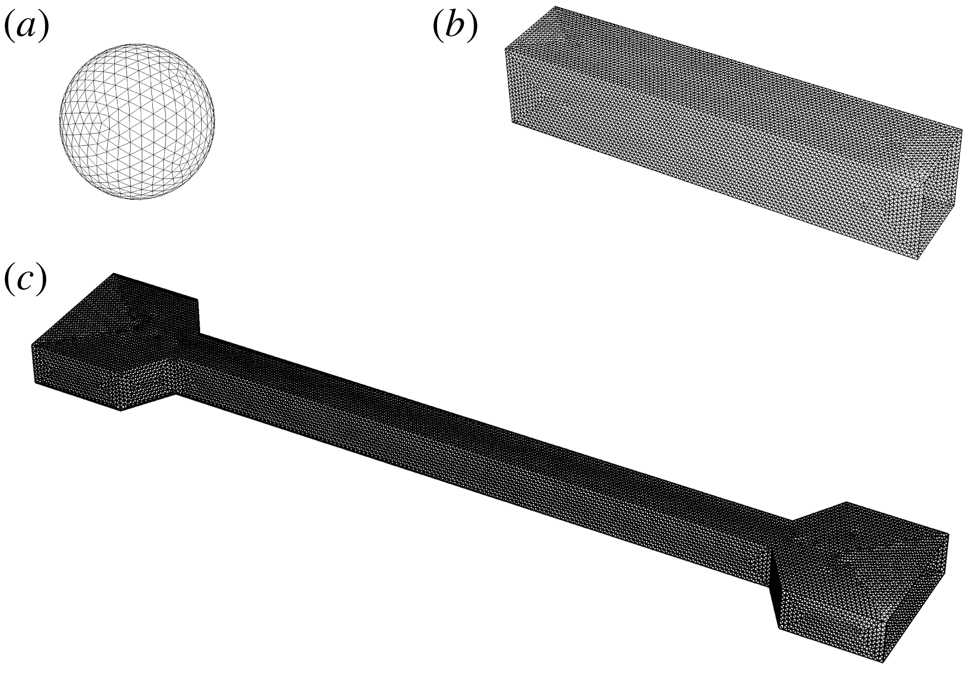
Unstructured surface meshes. (a) Vesicle surface
 $\mathscr{S}_{s}$
for a sphere-like vesicle, generated by subdividing an icosahedron. (b) Wall surface
 $\mathscr{S}_{w}$
for a straight conduit with a square cross-section. (c) Wall surface
 $\mathscr{S}_{w}$
for a contraction–expansion channel; the inlet and outlet are connected by a straight conduit with a square cross-section.

The present BEM implementation is completely general for arbitrary geometries, and here it is applied to the study of polygonal ducts with
 $N$
sides. Some of the unstructured meshes used in this paper are shown in figure 2 for
 $N=4$
(square ducts). The vesicle surface mesh is obtained by subdividing an icosahedron (figure 2
a); for lower reduced volumes, this surface is mapped onto a prolate spheroid. For the wall mesh, both a straight-channel geometry (figure 2
b) as well as a contraction–expansion geometry (figure 2
c) are used. The latter type of geometry is a realistic model for the microfluidic device used in the complementary experiments. The contraction–expansion geometry will be used to determine the time to reach a fully developed state, which can then be compared to results obtained for infinitely long channels.
Since bending elasticity has been neglected and the viscosity ratio
 $\unicode[STIX]{x1D705}$
has been set equal to unity, the family of solutions is parametrized by the reduced volume
 $\unicode[STIX]{x1D710}$
and radius ratio
 $\unicode[STIX]{x1D706}$
. Experimental measurements of the dimensionless extra pressure drop
 $\unicode[STIX]{x0394}p^{+}R/(\unicode[STIX]{x1D707}V)$
typically require very small membrane–wall separation distances in order to achieve a good signal-to-noise ratio. As will later be shown in § 5, the vesicles studied experimentally are highly confined, at radius ratios
 $\unicode[STIX]{x1D706}$
much higher than that which is easily determined via 3-D BEM simulation. Lubrication layers result in ill-conditioning of the collocation matrix, and the hydrodynamic interaction between the membrane and channel wall becomes difficult to resolve with acceptable accuracy. This restriction suggests the use of an alternative approach in order to predict the motion of vesicles at high confinement, which is the subject of the next section.
4 Lubrication theory
The lubrication approximation is a powerful method of regularizing the stress singularity that emerges when the distance between two boundaries separated by a viscous, flowing fluid becomes small compared to the lateral distance travelled by the fluid (Batchelor Reference Batchelor1967). It is expected that regions of high stress become concentrated in these narrow gaps. A reasonable question to ask is, how large can the vesicle be and still fit inside the duct without rupturing? Barakat & Shaqfeh (Reference Barakat and Shaqfeh2018b
) considered this problem for a circular-tube geometry, showing that the maximum radius ratio
 $\unicode[STIX]{x1D706}^{\ast }$
is related to the reduced volume
 $\unicode[STIX]{x1D710}$
by the geometric constraint,
 $$\begin{eqnarray}2\unicode[STIX]{x1D710}\unicode[STIX]{x1D706}^{\ast 3}-3\unicode[STIX]{x1D706}^{\ast 2}+1=0\quad \text{(circular tubes)}.\end{eqnarray}$$
Equation (4.1) is a simple cubic equation for
 $\unicode[STIX]{x1D706}^{\ast }$
that can be derived by first assuming the vesicle is a spherocylinder (the duct-conforming shape of the vesicle in a circular tube), and then requiring that the radius of the spherocylinder be equal to the channel hydraulic radius
 $R$
. By computing the surface area and volume of this shape, it is only a matter of algebra to arrive at (4.1). Significantly, the narrow-gap approximation considered by Barakat & Shaqfeh (Reference Barakat and Shaqfeh2018b
) for closely fitting vesicles in circular tubes is expected to be valid when the quantity
 $(1-\unicode[STIX]{x1D706}/\unicode[STIX]{x1D706}^{\ast })$
is small compared to unity.
For the square-duct geometry, the problem of determining the maximum vesicle size to fit inside the duct is not so simple because a spherocylindrical vesicle shape no longer conforms to the wall boundary. Nevertheless, one expects that there is indeed a critical radius ratio
 $\unicode[STIX]{x1D706}^{\ast }$
– at fixed reduced volume
 $\unicode[STIX]{x1D710}$
– that must be larger than
 $\unicode[STIX]{x1D706}$
if the vesicle is to fit inside the duct. Furthermore, one expects that this critical value
 $\unicode[STIX]{x1D706}^{\ast }$
exceeds the analogous value for the circular-tube geometry, due to the larger available cross-sectional area
 $A_{\times }$
. It is not the objective of the present study to calculate
 $\unicode[STIX]{x1D706}^{\ast }$
exactly for any reduced volume, nor is it the objective to develop a rigorous perturbation theory for
 $(1-\unicode[STIX]{x1D706}/\unicode[STIX]{x1D706}^{\ast })\ll 1$
. Without performing such calculations, some of the salient features of a maximally sized vesicle in a square conduit can be deduced from simple physical intuition:
(i) At the point of critical confinement
$\unicode[STIX]{x1D706}=\unicode[STIX]{x1D706}^{\ast }$
, portions of the vesicle membrane make ‘apparent contact’ with the duct boundary. Other portions of the membrane are ‘free’.(ii) The area of contact
$A^{\ast }$
between the membrane and the duct wall at
$\unicode[STIX]{x1D706}=\unicode[STIX]{x1D706}^{\ast }$
depends on the reduced volume
$\unicode[STIX]{x1D710}$
. For example, at
$\unicode[STIX]{x1D710}=1$
(a spherical vesicle), it is obvious that the critical radius ratio is
$\unicode[STIX]{x1D706}^{\ast }=1$
and membrane–wall contact is concentrated at four points. As
$\unicode[STIX]{x1D710}$
decreases from unity, these points of contact grow into surfaces.(iii) At some reduced volume
$\unicode[STIX]{x1D710}$
below unity, the vesicle would presumably fill the entire space and occlude flow through the duct. Complete occlusion is clearly forbidden since the membrane would have infinite curvature at the corners of the duct. Wong, Morris & Radke (Reference Wong, Morris and Radke1992), Wong, Radke & Morris (Reference Wong, Radke and Morris1995a
,Reference Wong, Radke and Morris
b
) showed that, for bubbles in polygonal capillaries, there is a cutoff length scale
$\unicode[STIX]{x1D6FC}^{-1}$
that sets the surface curvature in the corner regions. A similar length scale most likely exists for vesicles of low reduced volume, although this is beyond the scope of the present study.


A conclusion that can be drawn from item (ii) above is that the applicability of the lubrication approximation to the study of vesicle flow through polygonal ducts strongly depends on the reduced volume
 $\unicode[STIX]{x1D710}$
and radius ratio
 $\unicode[STIX]{x1D706}$
, because these parameters affect the available contact area
 $A^{\ast }$
. Significantly, when
 $\unicode[STIX]{x1D710}$
is close to unity, then the vesicle is quasi-spherical and the region of lubrication is concentrated at points. Since the study of O’Neill & Stewartson (Reference O’Neill and Stewartson1967) on the motion of rigid spheres translating parallel to plane walls, it has been well known that lubrication theory provides an accurate description of the local flow in the region of lubrication. However, the theory provides an inaccurate measure of global figures of merit (e.g. forces and force moments on a particle) when the region of lubrication is concentrated at a point and not a surface. The failure of lubrication theory can be attributed to the strength of the surface force density (measured in units of
 $\unicode[STIX]{x1D707}V/R$
) in comparison with the surface area (measured in units of
 $R^{2}$
). In the region of lubrication, the contact area
 $A^{\ast }$
is small, say
 $O(\unicode[STIX]{x1D716})$
with
 $\unicode[STIX]{x1D716}=1-\unicode[STIX]{x1D706}/\unicode[STIX]{x1D706}^{\ast }\ll 1$
, whereas the surface traction diverges, say with strength
 $O(\unicode[STIX]{x1D716}^{-1})$
. The overall force moment is then
 $O(1)$
. In the bulk region (outside the lubrication zone), the traction is
 $O(1)$
and the particle surface area is also
 $O(1)$
, giving an additional
 $O(1)$
contribution to the force moment. Since the lubrication and bulk regions are of comparable magnitude, both are significant to the calculation of integral hydrodynamic quantities. In relation to the present study, this means that lubrication theory is expected to supply a poor approximation of the dimensionless extra pressure drop
 $\unicode[STIX]{x0394}p^{+}R/(\unicode[STIX]{x1D707}V)$
– which, by (2.10), is computed from a force integral over the wall surface – when the reduced volume
 $\unicode[STIX]{x1D710}$
is very close to unity.
The aforementioned errors introduced through the lubrication approximation are eliminated when the duct cross-section is not a regular polygon but rather a circle. In the latter case, the region of lubrication between a large spherical particle and the duct boundary is concentrated at a contour (not a point) spanning the circumference of the cross-section. Consequently, a sphere translating through a circular tube has
 $O(\unicode[STIX]{x1D716}^{1/2})$
contact area with the wall and the resulting force moment is
 $O(\unicode[STIX]{x1D716}^{-1/2})$
, a singular contribution for
 $\unicode[STIX]{x1D716}\ll 1$
. For this reason, lubrication theory can provide an accurate approximation of the dimensionless extra pressure drop
 $\unicode[STIX]{x0394}p^{+}R/(\unicode[STIX]{x1D707}V)$
if the cross-section of the channel is circular and the vesicle is sufficiently large. The success of the lubrication approximation in predicting vesicle motion within the circular-tube geometry was previously verified by two of the authors through direct comparison to BEM simulations (Barakat & Shaqfeh Reference Barakat and Shaqfeh2018a
).
The above scaling arguments hold if
 $\unicode[STIX]{x1D710}$
is close to unity – that is, the vesicle is nearly spherical. However, the situation again qualitatively changes when
 $\unicode[STIX]{x1D710}<1$
. In this case, the apparent contact area
 $A^{\ast }$
is
 $O(1)$
, provided that
 $\unicode[STIX]{x1D706}$
is sufficiently close to
 $\unicode[STIX]{x1D706}^{\ast }$
. The lubrication contribution to the integral force moment is then
 $O(\unicode[STIX]{x1D716}^{-1})$
, rather than
 $O(\unicode[STIX]{x1D716}^{-1/2})$
as in the case for a quasi-spherical vesicle. This result was shown by Barakat & Shaqfeh (Reference Barakat and Shaqfeh2018b
) for vesicles in circular tubes – the dimensionless extra pressure drop
 $\unicode[STIX]{x0394}p^{+}R/(\unicode[STIX]{x1D707}V)$
was shown to diverge like
 $\unicode[STIX]{x1D716}^{-1/2}$
for spherical vesicles and like
 $\unicode[STIX]{x1D716}^{-1}$
for spherocylindrical vesicles at conditions of maximal confinement. In both of these cases, the ‘excess’ relative velocity
 $U/V-1$
is
 $O(\unicode[STIX]{x1D716})$
and always positive, with a coefficient that depends on the vesicle shape at steady state. For vesicles in the square-duct geometry considered in the present work, it is expected that lubrication theory provides the leading-order approximation, with errors that diminish as the apparent-contact area
 $A^{\ast }$
increases (i.e. the reduced volume
 $\unicode[STIX]{x1D710}$
decreases). However, one also expects the membrane surface flow to be non-uniform, unlike in the circular-tube geometry. This effect can have two significant consequences. For one, the presence of non-uniform surface flow changes the shear stresses in the gap and hence the dimensionless extra pressure drop
 $\unicode[STIX]{x0394}p^{+}R/(\unicode[STIX]{x1D707}V)$
. The ability of the flow to bypass the vesicle through the corner regions suggests that the extra pressure drop will be weaker in the square-duct geometry as compared to circular tubes. Second, the backflow in the region of lubrication indicates the possibility of the excess relative velocity
 $U/V-1$
being negative. That is to say, a sufficiently large vesicle could travel at a velocity
 $U$
slower than that of the mean flow
 $V$
in a square duct.
The above discussion motivates the development of a lubrication theory for the theoretical problem posed in § 2, which is the primary focus of this section. A similar approach to the one taken here was adopted in a previous study by two of the authors for circular tubes (Barakat & Shaqfeh Reference Barakat and Shaqfeh2018a
). In that study, the geometry considered was axisymmetric and the resulting equations coupling fluid flow to shape deformation were one-dimensional along the tube axis
 $x$
. In the present work, symmetry breaking induced by the duct geometry precludes the use of an axisymmetric theory. Rather, one must consider flow in both the axial and circumferential directions.
4.1 Formulation
Cylindrical coordinates
 $(\unicode[STIX]{x1D70C},\unicode[STIX]{x1D719},x)$
are conveniently adopted here, with
 $\unicode[STIX]{x1D70C}=\sqrt{y^{2}+z^{2}}$
being the radial distance,
 $\unicode[STIX]{x1D719}=\arctan (z/y)$
the azimuthal angle and
 $x$
the axial distance. The theory will be generally formulated for a polygonal duct with
 $N$
sides at steady state, assuming that the system has
 $N$
-fold symmetry (i.e. the geometry possesses reflectional symmetry at the planes
 $\unicode[STIX]{x1D719}=j\unicode[STIX]{x03C0}/N$
,
 $j=1,2,\ldots ,2N$
). Unlike in § 3, where the vesicle was given a Lagrangian representation, in the forthcoming development the surface position vector
 $\boldsymbol{x}_{s}$
will be given the Eulerian representation,
 $$\begin{eqnarray}x_{si}(\unicode[STIX]{x1D719},x)=x\unicode[STIX]{x1D6FF}_{1i}+\unicode[STIX]{x1D70C}_{s}(\unicode[STIX]{x1D719},x)\cos \unicode[STIX]{x1D719}\unicode[STIX]{x1D6FF}_{2i}+\unicode[STIX]{x1D70C}_{s}(\unicode[STIX]{x1D719},x)\sin \unicode[STIX]{x1D719}\unicode[STIX]{x1D6FF}_{3i},\end{eqnarray}$$
where
 $\unicode[STIX]{x1D70C}=\unicode[STIX]{x1D70C}_{s}(\unicode[STIX]{x1D719},x)$
defines the location of the vesicle membrane in space. The basic assumption of lubrication theory is to neglect components and gradients of velocity in the
 $\unicode[STIX]{x1D719}$
and
 $x$
directions. This assumption is rooted in assuming that spatial variations in the velocity field are most rapid in the transverse (
 $\unicode[STIX]{x1D70C}$
) direction as compared to the lateral (
 $\unicode[STIX]{x1D719}$
,
 $x$
) directions. In this approximation, the relevant velocity components
 $u_{\unicode[STIX]{x1D719}}$
and
 $u_{x}$
are governed by the simplified equations of motion,
 $$\begin{eqnarray}\displaystyle & \displaystyle \frac{\unicode[STIX]{x2202}p}{\unicode[STIX]{x2202}\unicode[STIX]{x1D70C}}=0, & \displaystyle\end{eqnarray}$$
 $$\begin{eqnarray}\displaystyle & \displaystyle \frac{\unicode[STIX]{x2202}p}{\unicode[STIX]{x2202}\unicode[STIX]{x1D719}}=\unicode[STIX]{x1D707}\unicode[STIX]{x1D70C}\frac{\unicode[STIX]{x2202}}{\unicode[STIX]{x2202}\unicode[STIX]{x1D70C}}\left(\frac{1}{\unicode[STIX]{x1D70C}}\frac{\unicode[STIX]{x2202}}{\unicode[STIX]{x2202}\unicode[STIX]{x1D70C}}(\unicode[STIX]{x1D70C}u_{\unicode[STIX]{x1D719}})\right), & \displaystyle\end{eqnarray}$$
 $$\begin{eqnarray}\displaystyle & \displaystyle \frac{\unicode[STIX]{x2202}p}{\unicode[STIX]{x2202}x}=\frac{\unicode[STIX]{x1D707}}{\unicode[STIX]{x1D70C}}\frac{\unicode[STIX]{x2202}}{\unicode[STIX]{x2202}\unicode[STIX]{x1D70C}}\left(\unicode[STIX]{x1D70C}\frac{\unicode[STIX]{x2202}u_{x}}{\unicode[STIX]{x2202}\unicode[STIX]{x1D70C}}\right), & \displaystyle\end{eqnarray}$$
 $$\begin{eqnarray}\displaystyle & \displaystyle u_{x}=u_{\unicode[STIX]{x1D719}}=0\quad \text{at }\unicode[STIX]{x1D70C}=R(\unicode[STIX]{x1D719}), & \displaystyle\end{eqnarray}$$
 $$\begin{eqnarray}\displaystyle & \displaystyle \unicode[STIX]{x1D707}\unicode[STIX]{x1D70C}\frac{\unicode[STIX]{x2202}}{\unicode[STIX]{x2202}\unicode[STIX]{x1D70C}}\left(\frac{u_{\unicode[STIX]{x1D719}}}{\unicode[STIX]{x1D70C}}\right)=-\frac{\unicode[STIX]{x2202}\unicode[STIX]{x1D70F}}{\unicode[STIX]{x2202}s_{\unicode[STIX]{x1D719}}}\quad \text{at }\unicode[STIX]{x1D70C}=\unicode[STIX]{x1D70C}_{s}(\unicode[STIX]{x1D719},x), & \displaystyle\end{eqnarray}$$
 $$\begin{eqnarray}\displaystyle & \displaystyle \unicode[STIX]{x1D707}\frac{\unicode[STIX]{x2202}u_{x}}{\unicode[STIX]{x2202}\unicode[STIX]{x1D70C}}=-\frac{\unicode[STIX]{x2202}\unicode[STIX]{x1D70F}}{\unicode[STIX]{x2202}s_{x}}\quad \text{at }\unicode[STIX]{x1D70C}=\unicode[STIX]{x1D70C}_{s}(\unicode[STIX]{x1D719},x). & \displaystyle\end{eqnarray}$$
 $\text{d}s_{\unicode[STIX]{x1D719}}=\sqrt{\unicode[STIX]{x1D70C}_{s}^{2}+(\unicode[STIX]{x2202}\unicode[STIX]{x1D70C}_{s}/\unicode[STIX]{x2202}\unicode[STIX]{x1D719})^{2}}\,\text{d}\unicode[STIX]{x1D719}$
and
 $\text{d}s_{x}=\sqrt{1+(\unicode[STIX]{x2202}\unicode[STIX]{x1D70C}_{s}/\unicode[STIX]{x2202}x)^{2}}\,\text{d}x$
are the arc lengths along the azimuth and channel axis, respectively. The local duct radius
 $R_{\unicode[STIX]{x1D719}}(\unicode[STIX]{x1D719})$
is given by
 $$\begin{eqnarray}R_{\unicode[STIX]{x1D719}}(\unicode[STIX]{x1D719})=R\sec \unicode[STIX]{x1D719},\quad 0\leqslant \unicode[STIX]{x1D719}\leqslant \frac{\unicode[STIX]{x03C0}}{N},\end{eqnarray}$$
where
 $N=4$
for a square duct. Due to symmetry, one need only consider the section of the domain bounded by
 $\unicode[STIX]{x1D719}=0$
and
 $\unicode[STIX]{x1D719}=\unicode[STIX]{x03C0}/N$
. It is expected that these equations supply a good approximation of the local flow conditions provided that
 $|\unicode[STIX]{x2202}\unicode[STIX]{x1D70C}_{s}/\unicode[STIX]{x2202}x|$
and
 $|\unicode[STIX]{x2202}\unicode[STIX]{x1D70C}_{s}/\unicode[STIX]{x2202}\unicode[STIX]{x1D719}|$
are not very large.
The pressure
 $p$
must be determined by conserving volume in the suspending fluid. (Consideration of the fluid inside the vesicle is immaterial, since the shear rates in the suspending fluid are presumably much larger than those in the interior fluid.) Depth-averaging the equation of continuity and applying the kinematic condition for a steady vesicle shape (
 $\boldsymbol{n}\boldsymbol{\cdot }\boldsymbol{u}=0$
on the membrane) yields a local mass balance condition,
 $$\begin{eqnarray}\frac{\unicode[STIX]{x2202}}{\unicode[STIX]{x2202}\unicode[STIX]{x1D719}}\left(\frac{q_{\unicode[STIX]{x1D719}}}{R}\right)+\frac{\unicode[STIX]{x2202}q_{x}}{\unicode[STIX]{x2202}x}=0,\end{eqnarray}$$
where
 $$\begin{eqnarray}q_{\unicode[STIX]{x1D719}}=\int _{\unicode[STIX]{x1D70C}_{s}(\unicode[STIX]{x1D719},x)}^{R_{\unicode[STIX]{x1D719}}(\unicode[STIX]{x1D719})}Ru_{\unicode[STIX]{x1D719}}\,\text{d}\unicode[STIX]{x1D70C},\quad q_{x}=\int _{\unicode[STIX]{x1D70C}_{s}(\unicode[STIX]{x1D719},x)}^{R_{\unicode[STIX]{x1D719}}(\unicode[STIX]{x1D719})}\unicode[STIX]{x1D70C}(u_{x}-U)\,\text{d}\unicode[STIX]{x1D70C}\end{eqnarray}$$
are the leakback fluxes (here, the factor of
 $R$
is introduced arbitrarily so that
 $q_{\unicode[STIX]{x1D719}}$
and
 $q_{x}$
have the same dimensions). Multiplying (4.6) by
 $\text{d}\unicode[STIX]{x1D719}$
, integrating from
 $\unicode[STIX]{x1D719}=0$
to
 $2\unicode[STIX]{x03C0}$
and applying periodicity conditions yields a macroscopic mass balance,
 $$\begin{eqnarray}\int _{0}^{2\unicode[STIX]{x03C0}}q_{x}\,\text{d}\unicode[STIX]{x1D719}=\int _{0}^{\unicode[STIX]{x03C0}/N}2Nq_{x}\,\text{d}\unicode[STIX]{x1D719}=Q-A_{\times }U=A_{\times }(V-U),\end{eqnarray}$$
where
 $$\begin{eqnarray}A_{\times }=\int _{0}^{\unicode[STIX]{x03C0}/N}NR_{\unicode[STIX]{x1D719}}^{2}\,\text{d}\unicode[STIX]{x1D719}\end{eqnarray}$$
is the cross-sectional surface area. Equation (4.8) holds for all
 $-L\leqslant x\leqslant 0$
, where
 $L$
is the length of the vesicle (a free boundary). Obviously, the velocities
 $U$
and
 $V$
cannot be specified independently. Rather, by specifying one, the other must be determined as part of the solution to the boundary-value problem. Here, it is most convenient to specify
 $U$
a priori and determine
 $V$
a posteriori.
The membrane tension
 $\unicode[STIX]{x1D70F}$
must also be determined, by conserving surface area locally on the membrane. This requirement is enforced by (2.4), which when written in cylindrical coordinates (with
 $\boldsymbol{n}\boldsymbol{\cdot }\boldsymbol{u}=0$
on the membrane) becomes
 $$\begin{eqnarray}\frac{1}{G_{s}}\frac{\unicode[STIX]{x2202}}{\unicode[STIX]{x2202}\unicode[STIX]{x1D719}}\left(\frac{G_{s}\bar{u}_{s\unicode[STIX]{x1D719}}}{\unicode[STIX]{x1D70C}_{s}}\right)+\frac{1}{G_{s}}\frac{\unicode[STIX]{x2202}}{\unicode[STIX]{x2202}x}(G_{s}\bar{u}_{sx})=0,\end{eqnarray}$$
where
 $G_{s}=\sqrt{\unicode[STIX]{x1D70C}_{s}^{2}[1+(\unicode[STIX]{x2202}\unicode[STIX]{x1D70C}_{s}/\unicode[STIX]{x2202}x)^{2}]+(\unicode[STIX]{x2202}\unicode[STIX]{x1D70C}_{s}/\unicode[STIX]{x2202}\unicode[STIX]{x1D719})^{2}}$
is the surface metric and
 $$\begin{eqnarray}\bar{u}_{s\unicode[STIX]{x1D719}}=u_{\unicode[STIX]{x1D719}}|_{\unicode[STIX]{x1D70C}=\unicode[STIX]{x1D70C}_{s}(\unicode[STIX]{x1D719},x)},\quad \bar{u}_{sx}=(u_{x}-U)|_{\unicode[STIX]{x1D70C}=\unicode[STIX]{x1D70C}_{s}(\unicode[STIX]{x1D719},x)}\end{eqnarray}$$
are the membrane slip velocities. Multiplying (4.10) by
 $G_{s}\,\text{d}\unicode[STIX]{x1D719}$
, integrating from
 $\unicode[STIX]{x1D719}=0$
to
 $2\unicode[STIX]{x03C0}$
and applying periodicity conditions gives
 $$\begin{eqnarray}\int _{0}^{2\unicode[STIX]{x03C0}}G_{s}\bar{u}_{sx}\,\text{d}\unicode[STIX]{x1D719}=\int _{0}^{\unicode[STIX]{x03C0}/N}2NG_{s}\bar{u}_{sx}\,\text{d}\unicode[STIX]{x1D719}=0.\end{eqnarray}$$
The right-hand side of (4.12) has been set equal to zero by the requirement that the vesicle remain stationary in the moving reference frame. This condition holds for all
 $-L\leqslant x\leqslant 0$
.
The equations (4.10)–(4.12) are exact at steady state, but require as input the local flow field
 $\boldsymbol{u}$
(cf. 4.7 and 4.11). The lubrication approximation allows one to analytically compute the flow field by considering only the dominant shear stresses in the
 $x\unicode[STIX]{x1D70C}$
and
 $\unicode[STIX]{x1D719}\unicode[STIX]{x1D70C}$
planes. Thus, expressions for the components of the leakback flux vector
 $\boldsymbol{q}$
and membrane slip velocity vector
 $\bar{\boldsymbol{u}}_{s}$
can be obtained directly by integrating (4.3)–(4.4) with respect to
 $\unicode[STIX]{x1D70C}$
:
 $$\begin{eqnarray}\displaystyle & \displaystyle \frac{q_{\unicode[STIX]{x1D719}}}{R}=\frac{m_{\unicode[STIX]{x1D719}}^{(qp)}}{\unicode[STIX]{x1D70C}_{s}}\frac{\unicode[STIX]{x2202}p}{\unicode[STIX]{x2202}\unicode[STIX]{x1D719}}+m_{\unicode[STIX]{x1D719}}^{(q\unicode[STIX]{x1D70F})}\frac{\unicode[STIX]{x2202}\unicode[STIX]{x1D70F}}{\unicode[STIX]{x2202}s_{\unicode[STIX]{x1D719}}},\quad q_{x}=m_{x}^{(qp)}\frac{\unicode[STIX]{x2202}p}{\unicode[STIX]{x2202}x}+m_{x}^{(q\unicode[STIX]{x1D70F})}\frac{\unicode[STIX]{x2202}\unicode[STIX]{x1D70F}}{\unicode[STIX]{x2202}s_{x}}-\frac{1}{2}U(R_{\unicode[STIX]{x1D719}}^{2}-\unicode[STIX]{x1D70C}_{s}^{2}), & \displaystyle\end{eqnarray}$$
 $$\begin{eqnarray}\displaystyle & \displaystyle \frac{\bar{u}_{s\unicode[STIX]{x1D719}}}{\unicode[STIX]{x1D70C}_{s}}=\frac{m_{\unicode[STIX]{x1D719}}^{(up)}}{\unicode[STIX]{x1D70C}_{s}}\frac{\unicode[STIX]{x2202}p}{\unicode[STIX]{x2202}\unicode[STIX]{x1D719}}+m_{\unicode[STIX]{x1D719}}^{(u\unicode[STIX]{x1D70F})}\frac{\unicode[STIX]{x2202}\unicode[STIX]{x1D70F}}{\unicode[STIX]{x2202}s_{\unicode[STIX]{x1D719}}},\quad \bar{u}_{sx}=m_{x}^{(up)}\frac{\unicode[STIX]{x2202}p}{\unicode[STIX]{x2202}x}+m_{x}^{(u\unicode[STIX]{x1D70F})}\frac{\unicode[STIX]{x2202}\unicode[STIX]{x1D70F}}{\unicode[STIX]{x2202}s_{x}}-U, & \displaystyle\end{eqnarray}$$
 $$\begin{eqnarray}\displaystyle & \displaystyle m_{\unicode[STIX]{x1D719}}^{(qp)}=-\frac{R_{\unicode[STIX]{x1D719}}^{3}}{8\unicode[STIX]{x1D707}}\left[\frac{\unicode[STIX]{x1D70C}_{s}}{R_{\unicode[STIX]{x1D719}}}-\frac{\unicode[STIX]{x1D70C}_{s}^{5}}{R_{\unicode[STIX]{x1D719}}^{5}}+\frac{4\unicode[STIX]{x1D70C}_{s}^{3}}{R_{\unicode[STIX]{x1D719}}^{3}}\log \left(\frac{\unicode[STIX]{x1D70C}_{s}}{R_{\unicode[STIX]{x1D719}}}\right)\right], & \displaystyle\end{eqnarray}$$
 $$\begin{eqnarray}\displaystyle & \displaystyle m_{\unicode[STIX]{x1D719}}^{(q\unicode[STIX]{x1D70F})}=-\frac{R_{\unicode[STIX]{x1D719}}^{2}}{4\unicode[STIX]{x1D707}}\left[\frac{\unicode[STIX]{x1D70C}_{s}^{2}}{R_{\unicode[STIX]{x1D719}}^{2}}-\frac{\unicode[STIX]{x1D70C}_{s}^{4}}{R_{\unicode[STIX]{x1D719}}^{4}}+\frac{2\unicode[STIX]{x1D70C}_{s}^{2}}{R_{\unicode[STIX]{x1D719}}^{2}}\log \left(\frac{\unicode[STIX]{x1D70C}_{s}}{R_{\unicode[STIX]{x1D719}}}\right)\right], & \displaystyle\end{eqnarray}$$
 $$\begin{eqnarray}\displaystyle & \displaystyle m_{x}^{(qp)}=-\frac{R_{\unicode[STIX]{x1D719}}^{4}}{16\unicode[STIX]{x1D707}}\left[\left(1-\frac{3\unicode[STIX]{x1D70C}_{s}^{2}}{R_{\unicode[STIX]{x1D719}}^{2}}\right)\left(1-\frac{\unicode[STIX]{x1D70C}_{s}^{2}}{R_{\unicode[STIX]{x1D719}}^{2}}\right)-\frac{4\unicode[STIX]{x1D70C}_{s}^{4}}{R_{\unicode[STIX]{x1D719}}^{4}}\log \left(\frac{\unicode[STIX]{x1D70C}_{s}}{R_{\unicode[STIX]{x1D719}}}\right)\right], & \displaystyle\end{eqnarray}$$
 $$\begin{eqnarray}\displaystyle & \displaystyle m_{x}^{(q\unicode[STIX]{x1D70F})}=\frac{R_{\unicode[STIX]{x1D719}}^{3}}{4\unicode[STIX]{x1D707}}\left[\frac{\unicode[STIX]{x1D70C}_{s}}{R_{\unicode[STIX]{x1D719}}}-\frac{\unicode[STIX]{x1D70C}_{s}^{3}}{R_{\unicode[STIX]{x1D719}}^{3}}+\frac{2\unicode[STIX]{x1D70C}_{s}^{3}}{R_{\unicode[STIX]{x1D719}}^{3}}\log \left(\frac{\unicode[STIX]{x1D70C}_{s}}{R_{\unicode[STIX]{x1D719}}}\right)\right], & \displaystyle\end{eqnarray}$$
 $$\begin{eqnarray}\displaystyle & \displaystyle m_{\unicode[STIX]{x1D719}}^{(up)}=\frac{R_{\unicode[STIX]{x1D719}}}{4\unicode[STIX]{x1D707}}\left[\frac{\unicode[STIX]{x1D70C}_{s}}{R_{\unicode[STIX]{x1D719}}}-\frac{\unicode[STIX]{x1D70C}_{s}^{3}}{R_{\unicode[STIX]{x1D719}}^{3}}+\frac{2\unicode[STIX]{x1D70C}_{s}}{R_{\unicode[STIX]{x1D719}}}\log \left(\frac{\unicode[STIX]{x1D70C}_{s}}{R_{\unicode[STIX]{x1D719}}}\right)\right], & \displaystyle\end{eqnarray}$$
 $$\begin{eqnarray}\displaystyle & \displaystyle m_{\unicode[STIX]{x1D719}}^{(u\unicode[STIX]{x1D70F})}=\frac{1}{2\unicode[STIX]{x1D707}}\left(1-\frac{\unicode[STIX]{x1D70C}_{s}^{2}}{R_{\unicode[STIX]{x1D719}}^{2}}\right), & \displaystyle\end{eqnarray}$$
 $$\begin{eqnarray}\displaystyle & \displaystyle m_{x}^{(up)}=-\frac{R_{\unicode[STIX]{x1D719}}^{2}}{4\unicode[STIX]{x1D707}}\left[1-\frac{\unicode[STIX]{x1D70C}_{s}^{2}}{R_{\unicode[STIX]{x1D719}}^{2}}+\frac{2\unicode[STIX]{x1D70C}_{s}^{2}}{R_{\unicode[STIX]{x1D719}}^{2}}\log \left(\frac{\unicode[STIX]{x1D70C}_{s}}{R_{\unicode[STIX]{x1D719}}}\right)\right], & \displaystyle\end{eqnarray}$$
 $$\begin{eqnarray}\displaystyle & \displaystyle m_{x}^{(u\unicode[STIX]{x1D70F})}=-\frac{\unicode[STIX]{x1D70C}_{s}}{\unicode[STIX]{x1D707}}\log \left(\frac{\unicode[STIX]{x1D70C}_{s}}{R_{\unicode[STIX]{x1D719}}}\right) & \displaystyle\end{eqnarray}$$
 $\unicode[STIX]{x1D707}$
,
 $\unicode[STIX]{x1D70C}_{s}$
and
 $R_{\unicode[STIX]{x1D719}}$
. Inserting (4.13) into (4.6) and (4.10) yields two second-order partial differential equations (PDEs) for the unknown fields
 $p$
and
 $\unicode[STIX]{x1D70F}$
:
 $$\begin{eqnarray}\displaystyle & & \displaystyle \frac{\unicode[STIX]{x2202}}{\unicode[STIX]{x2202}\unicode[STIX]{x1D719}}\left(\frac{m_{\unicode[STIX]{x1D719}}^{(qp)}}{\unicode[STIX]{x1D70C}_{s}}\frac{\unicode[STIX]{x2202}p}{\unicode[STIX]{x2202}\unicode[STIX]{x1D719}}\right)+\frac{\unicode[STIX]{x2202}}{\unicode[STIX]{x2202}x}\left(m_{x}^{(qp)}\frac{\unicode[STIX]{x2202}p}{\unicode[STIX]{x2202}x}\right)\nonumber\\ \displaystyle & & \displaystyle \quad +\,\frac{\unicode[STIX]{x2202}}{\unicode[STIX]{x2202}\unicode[STIX]{x1D719}}\left(m_{\unicode[STIX]{x1D719}}^{(q\unicode[STIX]{x1D70F})}\frac{\unicode[STIX]{x2202}\unicode[STIX]{x1D70F}}{\unicode[STIX]{x2202}s_{\unicode[STIX]{x1D719}}}\right)+\frac{\unicode[STIX]{x2202}}{\unicode[STIX]{x2202}x}\left(m_{x}^{(q\unicode[STIX]{x1D70F})}\frac{\unicode[STIX]{x2202}\unicode[STIX]{x1D70F}}{\unicode[STIX]{x2202}s_{x}}\right)=\frac{\unicode[STIX]{x2202}}{\unicode[STIX]{x2202}x}\left[\frac{1}{2}U(R_{\unicode[STIX]{x1D719}}^{2}-\unicode[STIX]{x1D70C}_{s}^{2})\right],\end{eqnarray}$$
 $$\begin{eqnarray}\displaystyle & & \displaystyle \frac{\unicode[STIX]{x2202}}{\unicode[STIX]{x2202}\unicode[STIX]{x1D719}}\left(\frac{G_{s}m_{\unicode[STIX]{x1D719}}^{(up)}}{\unicode[STIX]{x1D70C}_{s}}\frac{\unicode[STIX]{x2202}p}{\unicode[STIX]{x2202}\unicode[STIX]{x1D719}}\right)+\frac{\unicode[STIX]{x2202}}{\unicode[STIX]{x2202}x}\left(G_{s}m_{x}^{(up)}\frac{\unicode[STIX]{x2202}p}{\unicode[STIX]{x2202}x}\right)\nonumber\\ \displaystyle & & \displaystyle \quad +\,\frac{\unicode[STIX]{x2202}}{\unicode[STIX]{x2202}\unicode[STIX]{x1D719}}\left(G_{s}m_{\unicode[STIX]{x1D719}}^{(u\unicode[STIX]{x1D70F})}\frac{\unicode[STIX]{x2202}\unicode[STIX]{x1D70F}}{\unicode[STIX]{x2202}s_{\unicode[STIX]{x1D719}}}\right)+\frac{\unicode[STIX]{x2202}}{\unicode[STIX]{x2202}x}\left(G_{s}m_{x}^{(u\unicode[STIX]{x1D70F})}\frac{\unicode[STIX]{x2202}\unicode[STIX]{x1D70F}}{\unicode[STIX]{x2202}s_{x}}\right)=\frac{\unicode[STIX]{x2202}}{\unicode[STIX]{x2202}x}(G_{s}U).\end{eqnarray}$$
Although these equations are linear in
 $p$
and
 $\unicode[STIX]{x1D70F}$
, the boundary-value problem is nonlinear because the membrane radius
 $\unicode[STIX]{x1D70C}_{s}$
must also be determined as part of the solution. The governing PDE for
 $\unicode[STIX]{x1D70C}_{s}$
is the normal stress balance condition on the membrane:
 $$\begin{eqnarray}\displaystyle & & \displaystyle \frac{1}{G_{s}^{3}}\left\{\unicode[STIX]{x1D70C}_{s}\frac{\unicode[STIX]{x2202}^{2}\unicode[STIX]{x1D70C}_{s}}{\unicode[STIX]{x2202}x^{2}}\left[\unicode[STIX]{x1D70C}_{s}^{2}+\left(\frac{\unicode[STIX]{x2202}\unicode[STIX]{x1D70C}_{s}}{\unicode[STIX]{x2202}\unicode[STIX]{x1D719}}\right)^{2}\right]+\unicode[STIX]{x1D70C}_{s}\frac{\unicode[STIX]{x2202}^{2}\unicode[STIX]{x1D70C}_{s}}{\unicode[STIX]{x2202}\unicode[STIX]{x1D719}^{2}}\left[1+\left(\frac{\unicode[STIX]{x2202}\unicode[STIX]{x1D70C}_{s}}{\unicode[STIX]{x2202}x}\right)^{2}\right]-2\unicode[STIX]{x1D70C}_{s}\frac{\unicode[STIX]{x2202}\unicode[STIX]{x1D70C}_{s}}{\unicode[STIX]{x2202}x}\frac{\unicode[STIX]{x2202}\unicode[STIX]{x1D70C}_{s}}{\unicode[STIX]{x2202}\unicode[STIX]{x1D719}}\frac{\unicode[STIX]{x2202}^{2}\unicode[STIX]{x1D70C}_{s}}{\unicode[STIX]{x2202}x\unicode[STIX]{x2202}\unicode[STIX]{x1D719}}\right.\nonumber\\ \displaystyle & & \displaystyle \quad -\left.\left(\frac{\unicode[STIX]{x2202}\unicode[STIX]{x1D70C}_{s}}{\unicode[STIX]{x2202}\unicode[STIX]{x1D719}}\right)^{2}\right\}-\frac{1}{G_{s}}=\frac{p}{\unicode[STIX]{x1D70F}}.\end{eqnarray}$$
The left-hand side of (4.17) is twice the mean curvature
 $2H$
expressed in cylindrical coordinates. The reference pressure is chosen to be the interior vesicle pressure (assumed spatially homogeneous), so that the pressure
 $p$
the right-hand side of (4.17) (approximately) reflects the jump in the normal component of the membrane surface traction.
Although, strictly speaking, the lubrication equations (4.15)–(4.17) are only valid in regions where the bounding surfaces are nearly parallel, two of the authors have previously found success in extending these equations outside the lubrication region under axisymmetric conditions (Barakat & Shaqfeh Reference Barakat and Shaqfeh2018a
). There is substantial literature precedent for this solution methodology in application to red blood cells (Secomb et al.
Reference Secomb, Skalak, Oozkaya and Gross1986) and bubbles (Ratulowski & Chang Reference Ratulowski and Chang1989) in axisymmetric geometries. The basic justification for applying (4.15)–(4.17) outside the regions of lubrication hinges on the assumption that errors made in approximating the flow field outside the lubrication zone are of little consequence to the shape deformation and force moment integrals. This assumption breaks down when the region of closest separation between the vesicle membrane and the duct wall degenerates to points, as was discussed at the beginning of this section. Thus, equations (4.15)–(4.17) are applied over the whole domain
 $-L\leqslant x\leqslant 0$
and
 $0\leqslant \unicode[STIX]{x1D719}\leqslant \unicode[STIX]{x03C0}/N$
.
Equations (4.15)–(4.17) are nonlinear, elliptic PDEs for the fields
 $p$
,
 $\unicode[STIX]{x1D70F}$
, and
 $\unicode[STIX]{x1D70C}_{s}$
. In applying these equations to the whole domain, boundary conditions are required at the planes
 $x=0$
,
 $x=-L$
,
 $\unicode[STIX]{x1D719}=0$
and
 $\unicode[STIX]{x1D719}=\unicode[STIX]{x03C0}/N$
. Simple geometric considerations yield the following conditions:
 $$\begin{eqnarray}\displaystyle & \displaystyle \text{at }\unicode[STIX]{x1D719}=0:\frac{\unicode[STIX]{x2202}\unicode[STIX]{x1D70C}_{s}}{\unicode[STIX]{x2202}\unicode[STIX]{x1D719}}=0,\quad \frac{\unicode[STIX]{x2202}p}{\unicode[STIX]{x2202}\unicode[STIX]{x1D719}}=0,\quad \frac{\unicode[STIX]{x2202}\unicode[STIX]{x1D70F}}{\unicode[STIX]{x2202}\unicode[STIX]{x1D719}}=0, & \displaystyle\end{eqnarray}$$
 $$\begin{eqnarray}\displaystyle & \displaystyle \text{at }\unicode[STIX]{x1D719}=\frac{\unicode[STIX]{x03C0}}{N}:\frac{\unicode[STIX]{x2202}\unicode[STIX]{x1D70C}_{s}}{\unicode[STIX]{x2202}\unicode[STIX]{x1D719}}=0,\quad \frac{\unicode[STIX]{x2202}p}{\unicode[STIX]{x2202}\unicode[STIX]{x1D719}}=0,\quad \frac{\unicode[STIX]{x2202}\unicode[STIX]{x1D70F}}{\unicode[STIX]{x2202}\unicode[STIX]{x1D719}}=0, & \displaystyle\end{eqnarray}$$
 $$\begin{eqnarray}\displaystyle & \displaystyle \text{at }x=0:\unicode[STIX]{x1D70C}_{s}=0,\quad \frac{\unicode[STIX]{x1D70C}_{s}}{G_{s}}\frac{\unicode[STIX]{x2202}\unicode[STIX]{x1D70C}_{s}}{\unicode[STIX]{x2202}x}=-1,\quad \frac{\unicode[STIX]{x2202}}{\unicode[STIX]{x2202}\unicode[STIX]{x1D719}}\left(\frac{p}{\unicode[STIX]{x1D70F}}\right)=0, & \displaystyle\end{eqnarray}$$
 $$\begin{eqnarray}\displaystyle & \displaystyle \text{at }x=-L:\unicode[STIX]{x1D70C}_{s}=0,\quad \frac{\unicode[STIX]{x1D70C}_{s}}{G_{s}}\frac{\unicode[STIX]{x2202}\unicode[STIX]{x1D70C}_{s}}{\unicode[STIX]{x2202}x}=+1,\quad \frac{\unicode[STIX]{x2202}}{\unicode[STIX]{x2202}\unicode[STIX]{x1D719}}\left(\frac{p}{\unicode[STIX]{x1D70F}}\right)=0. & \displaystyle\end{eqnarray}$$
 $x$
(say,
 $x=-L/2$
) in order to conserve the total rate of flow of volume and surface area. The vesicle volume
 $\unicode[STIX]{x1D6FA}_{0}$
and surface area
 $A_{0}$
are related to
 $\unicode[STIX]{x1D70C}_{s}$
by the integral equations
 $$\begin{eqnarray}\displaystyle & \displaystyle \unicode[STIX]{x1D6FA}_{0}=\int _{0}^{\unicode[STIX]{x03C0}/N}\int _{-L}^{0}N\unicode[STIX]{x1D70C}_{s}^{2}\,\text{d}x\,\text{d}\unicode[STIX]{x1D719}, & \displaystyle\end{eqnarray}$$
 $$\begin{eqnarray}\displaystyle & \displaystyle A_{0}=\int _{0}^{\unicode[STIX]{x03C0}/N}\int _{-L}^{0}2NG_{s}\,\text{d}x\,\text{d}\unicode[STIX]{x1D719}, & \displaystyle\end{eqnarray}$$
which must be satisfied simultaneously with (4.8), (4.12) and (4.15)–(4.18). The boundary-value problem is now closed. Once a solution for the fields
 $p$
,
 $\unicode[STIX]{x1D70F}$
and
 $\unicode[STIX]{x1D70C}_{s}$
is obtained, the extra pressure drop
 $\unicode[STIX]{x0394}p^{+}$
is approximated by the difference in total pressure at the planes tangent to the front and rear ends of the vesicle:
 $$\begin{eqnarray}\unicode[STIX]{x0394}p^{+}\simeq \frac{1}{A_{\times }}\int _{0}^{\unicode[STIX]{x03C0}/N}NR_{\unicode[STIX]{x1D719}}^{2}(p|_{x=-L}-p|_{x=0})\,\text{d}\unicode[STIX]{x1D719}-LK_{hyd}A_{\times }V.\end{eqnarray}$$
The second term on the right-hand side is the Poiseuille pressure drop across a vesicle length
 $L$
. For a circular tube of radius
 $R$
, this contribution is equal to
 $8\unicode[STIX]{x1D707}VL/R^{2}$
. For a square duct (
 $N=4$
), it is
 $7.12\unicode[STIX]{x1D707}VL/R^{2}$
.
It is noteworthy that, although the derivation above was performed for a conduit whose cross-section is a polygon with
 $N$
sides, in principle this derivation could be applied to any cross-section. The applicability of the lubrication solution, however, is inherently dependent on the validity of neglecting additional viscous stresses in (4.3)–(4.4). The limitations of this assumption are discussed above.
As is common for problems in cylindrical coordinates, polar singularities occur at
 $x=0$
and
 $-L$
, resulting in a divergence of the membrane slope
 $|\unicode[STIX]{x2202}\unicode[STIX]{x1D70C}_{s}/\unicode[STIX]{x2202}x|\sim |x|^{-1/2}$
near these points. Following Wong et al. (Reference Wong, Morris and Radke1992), a coordinate transformation removes the polar singularity:
 $$\begin{eqnarray}\displaystyle x=-\frac{L}{2}(1-\cos \unicode[STIX]{x1D709}),\quad \unicode[STIX]{x1D709}=\arccos \left(1+\frac{2x}{L}\right), & & \displaystyle\end{eqnarray}$$
where
 $0\leqslant \unicode[STIX]{x1D709}\leqslant \unicode[STIX]{x03C0}$
. The coordinate transformation (4.22) has the additional benefit of clustering grid points near
 $x=0$
and
 $x=-L$
, which in turn enables resolution of sharp gradients near the poles. Conversion between
 $x$
- and
 $\unicode[STIX]{x1D709}$
-operations (i.e. derivatives and integrals) is easily achieved via the chain rule. In the transformed domain, the polar singularity is removed by application of l’Hôpital’s rule (Wong et al.
Reference Wong, Morris and Radke1992). However, two additional concerns remain. Firstly, removing the polar singularity does nothing to alleviate the additional stress singularity that results from the failure of the lubrication approximation at the poles. Although this latter kind of singularity cannot be removed, it is of little consequence to the solution of the boundary-value problem. The stresses computed via lubrication theory diverge within a very small region near the front nose and rear tail of the vesicle, and hence their overall contribution to the shape deformation and force moment integrals is negligible. Secondly, the one-to-one mapping between
 $x$
and
 $\unicode[STIX]{x1D709}$
excludes the possibility of multivalued solutions to the boundary-value problem. Such solutions can occur, for instance, when the vesicle develops concave curvature in the rear end (the so-called ‘parachute shape’). This restriction is somewhat mild, however, as the vesicles considered in the present work have reduced volumes in the range
 $0.85\leqslant \unicode[STIX]{x1D710}\leqslant 1$
. Such vesicles are approximately spherical and do not typically develop concave curvature under flow.
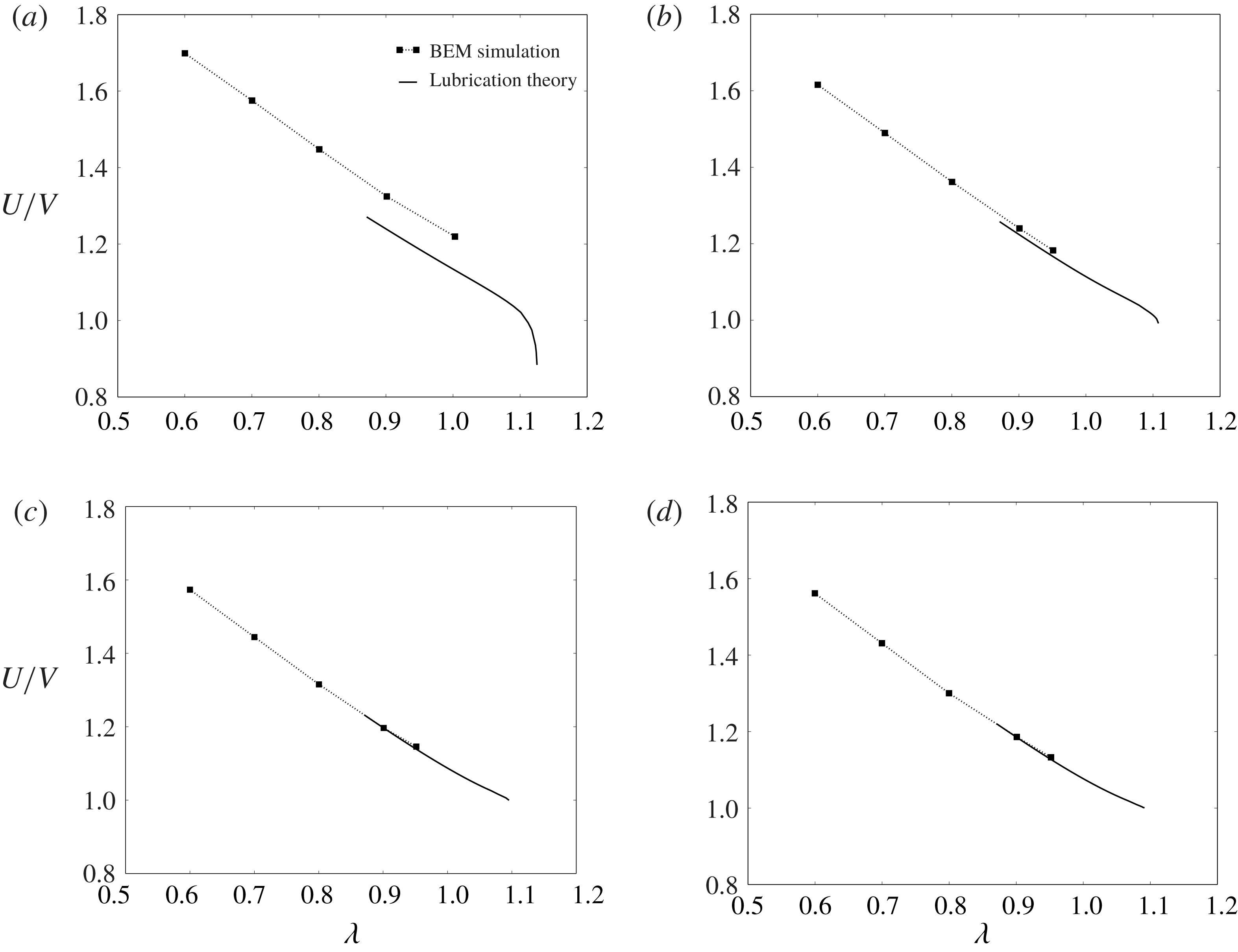
Relative velocity
 $U/V$
plotted against the radius ratio
 $\unicode[STIX]{x1D706}$
for
 $\unicode[STIX]{x1D710}=0.99$
and (a)
 $N=4$
(square), (b)
 $N=6$
(hexagon), (c)
 $N=12$
(dodecagon) and (d)
 $N\rightarrow \infty$
(circle). The symbols are the BEM simulations, while the solid lines are the predictions from lubrication theory.

Equations (4.8), (4.12) and (4.15)–(4.20) were solved using the finite difference method. The poles
 $\unicode[STIX]{x1D709}=0$
and
 $\unicode[STIX]{x03C0}$
were excluded from the domain in order to avoid the stress singularity at these points. The membrane shape at the poles was approximated by a spherical section with constant curvature. The 2-D domain was discretized into a uniform grid and second-order accurate spatial difference operators were used to approximate derivatives and integrals with respect to
 $\unicode[STIX]{x1D719}$
and
 $\unicode[STIX]{x1D709}$
. Applying the difference analogy to the governing equations (4.8), (4.12) and (4.15)–(4.20) results in a system of nonlinear algebraic equations, which was subsequently solved iteratively using a Newton–Raphson procedure. For each Newton step, the Jacobian matrix was pre-computed analytically and subsequently discretized using finite differences. Iteration proceeded until the merit function to be zeroed fell below
 $10^{-6}$
or the Newton step in the descent direction fell below
 $10^{-6}$
. Starting from some initial guess (e.g. solutions of the analogous axisymmetric problem considered by Barakat & Shaqfeh (Reference Barakat and Shaqfeh2018a
)), convergence was typically achieved in under 10 iterations. A family of solutions parametrized by
 $\unicode[STIX]{x1D710}$
and
 $\unicode[STIX]{x1D706}$
was obtained using the continuation method. Typically, higher spatial resolution was necessary in order to achieve convergence for large values of
 $\unicode[STIX]{x1D706}$
. For further details on the numerical method, the reader is referred to Barakat (Reference Barakat2018).
Dimensionless extra pressure drop
 $\unicode[STIX]{x0394}p^{+}R/(\unicode[STIX]{x1D707}V)$
plotted against the radius ratio
 $\unicode[STIX]{x1D706}$
for
 $\unicode[STIX]{x1D710}=0.99$
and (a)
 $N=4$
(square), (b)
 $N=6$
(hexagon), (c)
 $N=12$
(dodecagon) and (d)
 $N\rightarrow \infty$
(circle). The symbols are the BEM simulations, while the solid lines are the predictions from lubrication theory.

4.2 Error analysis
The lubrication approximation is not an exact solution of Stokes’ equations of motion. Viscous stresses induced by velocity gradients neglected in the approximation can contribute to the momentum flux in the
 $x$
and
 $\unicode[STIX]{x1D719}$
directions. These stresses are not expected to contribute significantly when the flow is axisymmetric. For the non-axisymmetric flow in square ducts, these stresses are expected to play a more significant role. There are large portions of the domain (e.g. the corners and the ends of the vesicle) where the gap separating the membrane and the duct wall is not narrow, nor is it slowly varying in the axial or circumferential directions. Consequently, while the local flow field in the narrow-gap region is expected to be well approximated by the lubrication theory, the macroscopic mass and momentum balances may incur substantial errors due to neglected viscous stresses, particularly for motion tangential to the wall (less so for normal motion, which is not considered here) (O’Neill & Stewartson Reference O’Neill and Stewartson1967). These errors are expected to decrease if the flow becomes axisymmetric, the narrow gap thins, or the apparent-contact area
 $A^{\ast }$
increases.
The macroscopic mass and momentum balances lead directly to the integral figures of merit: the relative velocity
 $U/V$
and dimensionless extra pressure drop
 $\unicode[STIX]{x0394}p^{+}R/(\unicode[STIX]{x1D707}V)$
. In order to estimate the errors made in the lubrication approximation, these quantities were computed at different values of
 $N$
(polygonal ducts with varying number of edges in a cross-section) and compared to the analogous BEM simulations. Results for the relative velocity
 $U/V$
and dimensionless extra pressure drop
 $\unicode[STIX]{x0394}p^{+}R/(\unicode[STIX]{x1D707}V)$
are shown in figures 3 and 4, respectively, for
 $N=4$
(square cross-section), 6 (hexagonal), 12 (dodecagonal) and
 $\infty$
(circular). From comparing the two methods, it is clear that the lubrication theory underpredicts both the relative velocity and extra pressure drop. The error is most significant for the square cross-section, and decreases as
 $N$
increases until the system approaches the cylindrically symmetric system. For the circular-tube case, the error in the relative velocity nearly vanishes, whereas there remains a very small error in the extra pressure drop. This error is likely due to the approximation (4.21), which neglects wall stresses upstream and downstream of the ends of the vesicle.
From figures 3 and 4, one may reasonably conclude that the errors in the lubrication approximation arise from the neglect of velocity gradients in the azimuthal direction (e.g.
 $\unicode[STIX]{x2202}u_{x}/\unicode[STIX]{x2202}\unicode[STIX]{x1D719}$
and
 $\unicode[STIX]{x2202}u_{\unicode[STIX]{x1D719}}/\unicode[STIX]{x2202}\unicode[STIX]{x1D719}$
) in the equations of motion and stress conditions. These terms are not necessarily small and should play a significant role when the duct is not axisymmetric. However, one expects that these terms become less important as the vesicle becomes more confined. As the radius ratio
 $\unicode[STIX]{x1D706}$
increases, the vesicle fills the entire cross-section and the gap separating the membrane from the duct wall becomes very small in certain regions. Velocity gradients with respect to the radial distance (e.g.
 $\unicode[STIX]{x2202}u_{x}/\unicode[STIX]{x2202}\unicode[STIX]{x1D70C}$
and
 $\unicode[STIX]{x2202}u_{\unicode[STIX]{x1D719}}/\unicode[STIX]{x2202}\unicode[STIX]{x1D70C}$
) are dominant in this case, and lubrication theory is expected to predict the singular contribution to integral force moments.
Unfortunately, it is not possible to compare the lubrication theory to the BEM simulations at very high confinement, since the BEM calculations become prohibitively expensive in this regime. Instead, the lubrication theory is compared to experimental measurements at similarly high confinement (delayed until § 6). Details of the experimental methods are given in the next section.
5 Experimental
A microfluidic manometer method, previously used to study the extra pressure drop across single droplets (Vanapalli et al.
Reference Vanapalli, Banpurkar, van den Ende, Duits and Mugele2009) and cells (Abkarian, Faivre & Stone Reference Abkarian, Faivre and Stone2006; Khan & Vanapalli Reference Khan and Vanapalli2013; Khan et al.
Reference Khan, Kamyabi, Hussain and Vanapalli2017) was adopted to simultaneously measure the relative velocity
 $U/V$
and dimensionless extra pressure drop
 $\unicode[STIX]{x0394}p^{+}R/(\unicode[STIX]{x1D707}V)$
. The manometer principle (illustrated in figure 5) involves applying a constant pressure at the inlets of the so-called reference and test channels, and recording the fluid–fluid interface deflection in the comparator region downstream as the vesicle passes through the test channel (Groisman, Enzelberger & Quake Reference Groisman, Enzelberger and Quake2003; Vanapalli et al.
Reference Vanapalli, Van den Ende, Duits and Mugele2007).
Working principle of the microfluidic manometer. Equal driving pressures are applied to a test channel (containing a single vesicle) and a reference channel (containing a clear fluid). The co-flowing fluids meet at a downstream comparator, forming a fluid–fluid interface. In the absence of a vesicle, the interface is flat (parallel to the streamwise direction). In the presence of a vesicle, a measurable displacement
 $\unicode[STIX]{x0394}Y$
is observed due to the excess flow resistance in the test channel.

Vesicles were synthesized using standard electroformation methods (Angelova et al.
Reference Angelova, Soléau, Méléard and Faucon1992; Ahmmed et al.
Reference Ahmmed, Suteria, Garbin and Vanapalli2018). The formulation consisted of 1-stearoyl-2-oleoyl-sn-glycero-3-phospho-choline (SOPC) and cholesterol at 1:1 molar ratio, or SOPC:Chol. The internal and suspending phase of the vesicles was 0.11 M sucrose and 0.12 M glucose solution respectively, with viscosities
 ${\approx}1~\text{mN}~\text{s}~\text{m}^{-2}$
. Due to optical limitations, the reduced volume
 $\unicode[STIX]{x1D710}$
could not be accurately measured during the microfluidic experiments. Literature precedent suggests a distribution of reduced volumes with a mean value of
 $\unicode[STIX]{x1D710}=0.98$
for SOPC:Chol vesicles prepared by electroformation (the standard deviation was not reported) (Pommella et al.
Reference Pommella, Brooks, Seddon and Garbin2015). It is expected that, without the addition of electrolytes to induce a small osmotic pressure difference, the vesicles prepared will have reduced volumes in the range
 $0.85\leqslant \unicode[STIX]{x1D710}\leqslant 1$
. The possibility of multilamellarity was not accounted for in this study.
The microfluidic manometer devices were fabricated using standard soft lithography techniques (Xia & Whitesides Reference Xia and Whitesides1998). The manometer design consisted of two square channels of
 $\text{width}\times \text{height}\times \text{length}=(12.6\pm 0.6)\times (12.8\pm 0.7)\times 330~\unicode[STIX]{x03BC}\text{m}$
, which meet downstream to form a comparator region of width
 $110~\unicode[STIX]{x03BC}\text{m}$
(figure 5). Vesicles were introduced into the test channel; in the reference channel, a 0.12 M glucose solution with a trace amount of black food dye was used to facilitate visualization of the deflected interface downstream. The pressure gradients in the channels were controlled using an electronic pressure controller system (MFCS, Fluigent Inc.). Imaging was conducted on an inverted microscope (IX 71, Olympus Inc.) in the phase contrast mode and images were acquired with a CMOS camera (Phantom v310, Vision Research) at an exposure time of
 $50~\unicode[STIX]{x03BC}\text{s}$
and a frame rate of 2000 f.p.s. The effective pixel size for this optical setup is
 $0.97~\unicode[STIX]{x03BC}\text{m}$
.
Prior to the vesicle experiments, a calibration curve was generated to relate the extra pressure drop
 $\unicode[STIX]{x0394}p^{+}$
to the interface displacement
 $\unicode[STIX]{x0394}Y$
, by varying the test channel driving pressure and capturing the corresponding interface displacement while keeping the reference channel driving pressure fixed. The interface displacement was obtained from the captured images by fitting an error function to the intensity values of a vertical row of pixels
 $10~\unicode[STIX]{x03BC}\text{m}$
away from the tip, where the two fluids first meet in the comparator. The true interface position was taken to be the midpoint between the lowest and highest grey-scale regions of the fitted curve. When a vesicle occludes the test channel, the flow rate in it is reduced and therefore the interface is displaced in the comparator region. The calibration curve enables one to directly map
 $\unicode[STIX]{x0394}Y$
to
 $\unicode[STIX]{x0394}p^{+}$
. One limitation of this method, as was mentioned at the end of § 3, is that the pressure drop must be sufficiently high in order to achieve a measurable deflection. As such, measurements of
 $\unicode[STIX]{x0394}p^{+}$
could only be obtained for sufficiently large radius ratios
 $\unicode[STIX]{x1D706}$
(typically greater than unity).
The vesicle translational velocity
 $U$
was measured manually using the ImageJ software package (v.1.6.0-24, NIH). For each experiment, the time taken for a vesicle to travel the channel length
 $(300~\unicode[STIX]{x03BC}\text{m})$
was recorded provided that the vesicle’s motion was steady. Using this transit time and travel distance, the vesicle velocity was computed (maximum error
 ${<}3\,\%$
, based on image resolution).
Independent experiments were performed in order to determine the mean fluid velocity
 $V$
during vesicle transport through the test channel. In the absence of vesicles, a flow rate
 $Q$
was imposed using a syringe pump (PHD 2000, Harvard Apparatus) in the test channel, with a constant pressure imposed at the inlet of the reference channel. The interface displacements were recorded as a function of the pump flow rate. Therefore, using the two curves
 $\unicode[STIX]{x0394}p^{+}$
versus
 $\unicode[STIX]{x0394}Y$
and
 $Q$
versus
 $\unicode[STIX]{x0394}Y$
, a one-to-one mapping between
 $\unicode[STIX]{x0394}p^{+}$
and
 $Q$
was obtained. Using this relationship, the mean fluid velocity
 $V$
in the presence of the vesicle was determined. The errors incurred due to the fact that the vesicle-free fluid has a smaller effective viscosity are expected to be small, since the additional viscosity imparted by the vesicle to the fluid is an
 $O(c)$
contribution (
 $c\ll 1$
being the volume fraction occupied by the vesicle in the fluid system). In all of the reported experiments, the applied pressure drop in the manometer was such that mean fluid velocities and shear rates (
 ${\sim}V/H$
) were
 $1.15{-}2.12~\text{cm}~\text{s}^{-1}$
and
 $750{-}1700~\text{s}^{-1}$
, respectively.
To calculate the radius ratio
 $\unicode[STIX]{x1D706}$
, the size of each vesicle was measured prior to entering the constriction (where a vesicle is assumed to have a ‘pancake’ shape due to the converging duct cross-section). Specifically, the projected area of the vesicle was measured using ImageJ and fitted to a circle (measurement error
 ${<}3\,\%$
due to image resolution); the volume and surface area were estimated by assuming the vesicle to be a body of revolution, as described by Vuong & Anna (Reference Vuong and Anna2012). From the surface area, the equivalent vesicle radius
 $R_{0}$
was computed and normalized by the channel hydraulic radius
 $R$
in order to obtain the radius ratio
 $\unicode[STIX]{x1D706}$
.
As stated previously, the reduced volume
 $\unicode[STIX]{x1D710}$
could not be accurately measured during the experiments. Estimating
 $\unicode[STIX]{x1D710}$
based on the ‘pancake’ model described above typically results in an overestimation (reduced volumes very close to unity). When the vesicle enters the narrow channel, the aspect ratio
 $L/(2R)$
is typically larger than unity, indicating that the vesicle is aspherical under confinement. The reduced volume was approximated by measuring the aspect ratio
 $L/(2R)$
and using the lubrication solutions of the vesicle shape at near-critical confinement in order to relate
 $L/(2R)$
to
 $\unicode[STIX]{x1D710}$
(discussed further in § 6.3, below).
(a) Time-stamped images showing vesicle motion in the test channel and the concomitant interface deflection. The test channel is approximately
 $12.6~\unicode[STIX]{x03BC}\text{m}$
wide and
 $330~\unicode[STIX]{x03BC}\text{m}$
long. (b) Time evolution of the relative velocity
 $U/V$
and dimensionless extra pressure drop
 $\unicode[STIX]{x0394}p^{+}R/(\unicode[STIX]{x1D707}V)$
for a vesicle of reduced volume
 $\unicode[STIX]{x1D710}$
near unity (
 $\unicode[STIX]{x1D706}=1.56$
).

A representative experiment is shown in figure 6. Figure 6(a) shows time-stamped images of a SOPC:Chol vesicle translating through the test channel and the induced interface deflection. From observation, the vesicle deforms at the constriction entrance but does not slow down as it penetrates into the channel. Figure 6(b) shows the associated time evolution of the relative velocity
 $U/V$
and dimensionless extra pressure drop
 $\unicode[STIX]{x0394}p^{+}R/(\unicode[STIX]{x1D707}V)$
as the vesicle translates through the channel. As expected, the extra pressure drop is nearly zero prior to the vesicle reaching the constriction entrance. Then, there is a sharp rise in the extra pressure drop, which reaches a maximum at a few channel diameters away from the constriction entrance. This maximum in the extra-pressure-drop signal is maintained, producing a plateau region until the vesicle reaches the channel exit. Thereafter, the extra pressure drop decreases and actually appears to be negative, since the presence of vesicle in the comparator region perturbs the interface location. For the purposes of comparing the measurements to the theoretical predictions, the mean value of the extra pressure drop in the plateau region was evaluated. The fluctuations in the plateau region were
 ${<}5\,\%$
for a large vesicle (
 $\unicode[STIX]{x1D706}\geqslant 1.3$
) and 5 %–10 % for smaller vesicles (
 $1<\unicode[STIX]{x1D706}<1.3$
). The time evolution of the relative velocity
 $U/V$
mirrors that of the extra pressure drop except that the rise in velocity occurred slightly earlier than the extra pressure drop. This delay is likely due to the response time of the manometer.
6 Discussion of results
In this section, the main results from the BEM simulations, lubrication theory and microfluidic experiments are presented for the motion of vesicles through square conduits. In § 4.2, it was shown that the lubrication approximation yields more significant errors in the square-duct geometry than in the circular-tube geometry, due to the importance of azimuthal stresses neglected in the approximation (these errors essentially disappear as the symmetry of the duct increases, i.e. as
 $N\rightarrow \infty$
). However, it is expected that this approximation yields the correct singular contribution to the relative velocity
 $U/V$
and dimensionless extra pressure drop
 $\unicode[STIX]{x0394}p^{+}R/(\unicode[STIX]{x1D707}V)$
as
 $\unicode[STIX]{x1D706}$
approaches a maximum. This information will be crucial when comparing to the experimental results.
6.1 Vesicle flow through a contraction
To begin, the BEM simulations for straight channels with square cross-section are compared to the contraction–expansion simulations. The goal here is to correlate the instantaneous vesicle confinement, relative velocity
 $U/V$
, and dimensionless extra pressure drop
 $\unicode[STIX]{x0394}p^{+}R/(\unicode[STIX]{x1D707}V)$
, as well as quantify the time to reach steady state.
(a) Time sequence of a vesicle (reduced volume
 $\unicode[STIX]{x1D710}=0.99$
) passing through a square constriction channel, as computed via BEM simulation. The left and right columns correspond to
 $\unicode[STIX]{x1D706}=0.6$
and
 $0.8$
, respectively. (b) Relative velocity
 $U/V$
and dimensionless extra pressure drop
 $\unicode[STIX]{x0394}p^{+}R/(\unicode[STIX]{x1D707}V)$
plotted against the dimensionless time
 $tV/R$
for
 $\unicode[STIX]{x1D710}=0.99$
and
 $\unicode[STIX]{x1D706}=0.6,0.8$
. The dashed, horizontal lines correspond to the steady-state results for an infinitely long, square conduit.

Figure 7 shows BEM simulation results for a nearly spherical vesicle (reduced volume
 $\unicode[STIX]{x1D710}=0.99$
) entering a constriction, at two different radius ratios (
 $\unicode[STIX]{x1D706}=0.6$
and 0.8). The mesh geometry (shown in figure 2
c) has the same dimensions as the ‘test channel’ of the microfluidic manometer (figures 5 and 6). The straight-channel portion of the geometry is sufficiently long such that the expansion flow downstream does not affect the vesicle motion. In the experiment shown in figure 6, the radius ratio
 $\unicode[STIX]{x1D706}$
is higher than that reported in figure 7. High-confinement simulations require an exorbitant number of mesh elements and are prohibitively costly with the current BEM implementation. As such, one should not directly compare figure 7 to figure 6. Nevertheless, the simulations can give insight into the transient effects at the entrance of the manometer, at lower confinement.
The vesicle shape (figure 7
a) is tracked together with the relative velocity
 $U/V$
and dimensionless extra pressure drop
 $\unicode[STIX]{x0394}p^{+}R/(\unicode[STIX]{x1D707}V)$
(figure 7
b). As the vesicle approaches the entrance of the narrow channel, it accelerates due to the converging flow field; the extra pressure drop rises simultaneously. At
 $tV/R=0$
, the vesicle enters the square duct and the pressure drop fluctuates; these fluctuations are dampened as confinement increases. Steady state is achieved after the vesicle travels several channel radii (roughly
 $tV/R\simeq 3$
), which is consistent with the experiment shown in figure 6 (physically, this distance is approximately
 $40~\unicode[STIX]{x03BC}\text{m}$
for a channel hydraulic radius of
 $12~\unicode[STIX]{x03BC}\text{m}$
). Increasing the flow confinement (
 $\unicode[STIX]{x1D706}$
) results in a slight reduction in the relative velocity
 $U/V$
and a dramatic increase in the dimensionless extra pressure drop
 $\unicode[STIX]{x0394}p^{+}R/(\unicode[STIX]{x1D707}V)$
. Similar trends are observed for lower reduced volumes (not shown here).
Quéguiner & Barthès-Biesel (Reference Quéguiner and Barthès-Biesel1997) performed BEM simulations of a capsule (a model for a red blood cell) entering an axisymmetric contraction–expansion geometry. These authors modelled the capsule membrane as either a neo-Hookean solid or as an incompressible sheet; the latter is equivalent to the membrane model used in the present study. They tracked the pressure drop as a function of distance travelled by the capsule and showed that a steady state was achieved after several channel radii, as is shown here. To the best of the authors’ knowledge, the present simulations are the first to model a vesicle flowing through rectangular contraction–expansion geometry, which is fully three-dimensional and hence cannot be investigated using the axisymmetric boundary integral equations.
6.2 Steady vesicle shapes, surface tractions and surface velocities
Figures 8–11 show the theoretical predictions for the vesicle shape in square conduits at two different reduced volumes (
 $\unicode[STIX]{x1D710}=0.99$
and
 $0.90$
) and a range of radius ratios
 $\unicode[STIX]{x1D706}$
. The images are ordered (top-to-bottom) with increasing radius ratio
 $\unicode[STIX]{x1D706}$
; thus, vesicle confinement increases down the page. The colours indicate the normal component of the membrane surface traction jump (i.e. the ‘total pressure’),
 $f_{sn}=\boldsymbol{n}\boldsymbol{\cdot }\boldsymbol{f}_{\!s}$
. Larger values of
 $f_{sn}$
(towards positively valued numbers) indicate higher pressures in the suspending fluid phase. The results shown in figures 8 and 10 were obtained using BEM simulations; those shown in figures 9 and 11 were obtained using lubrication theory. In order to compare results from the BEM and lubrication theory, one may juxtapose figures 8(d) and 9(a) (for
 $\unicode[STIX]{x1D710}=0.99$
,
 $\unicode[STIX]{x1D706}=0.9$
), as well as figures 10(e) and 11(a) (for
 $\unicode[STIX]{x1D710}=0.90$
,
 $\unicode[STIX]{x1D706}=1.1$
). Clearly, the two methods produce qualitatively similar shapes and pressure distributions. Quantitative differences in the computed pressures are also observed.
Vesicles (
 $\unicode[STIX]{x1D710}=0.99$
) in square ducts as determined by 3-D BEM simulation, viewed from
 $yz$
(left) and
 $xy$
(right) planes. The colours indicate the normal component of the membrane surface traction jump
 $f_{sn}=\boldsymbol{n}\boldsymbol{\cdot }\boldsymbol{f}_{s}$
. Shown are results for
 $\unicode[STIX]{x1D706}=$
(a) 0.6, (b) 0.7, (c) 0.8 and (d) 0.9.

Vesicles (
 $\unicode[STIX]{x1D710}=0.99$
) in square ducts as determined by lubrication theory, viewed from
 $yz$
(left) and
 $xy$
(right) planes. The colours have the same meaning as in figure 8. Shown are results for
 $\unicode[STIX]{x1D706}=$
(a) 0.9, (b) 1.0, (c) 1.1 and (d) 1.12.

Vesicles (
 $\unicode[STIX]{x1D710}=0.90$
) in square ducts as determined by 3-D BEM simulation, viewed from
 $yz$
(left) and
 $xy$
(right) planes. The colours indicate the normal component of the membrane surface traction jump
 $f_{sn}=\boldsymbol{n}\boldsymbol{\cdot }\boldsymbol{f}_{s}$
. Shown are results for
 $\unicode[STIX]{x1D706}=$
(a) 0.7, (b) 0.8, (c) 0.9, (d) 1.0 and (e) 1.1.

Vesicles (
 $\unicode[STIX]{x1D710}=0.90$
) in square ducts as determined by lubrication theory, viewed from
 $yz$
(left) and
 $xy$
(right) planes. The colours have the same meaning as in figure 10. Shown are results for
 $\unicode[STIX]{x1D706}=$
(a) 1.1, (b) 1.2, (c) 1.3, (d) 1.4 and (e) 1.43.

Figures 8(a), 10(a) show that the pressure distribution in the vicinity of the vesicle surface is nearly axisymmetric at low flow confinement. Were the vesicle to shrink to a point, local analysis of the flow field in a square duct yields an axisymmetric flow field at the channel centreline. Finite-sized vesicles sample a non-axisymmetric flow field. Figure 10(a,b) shows a fourfold symmetric ‘parachute shape’ for
 $\unicode[STIX]{x1D710}=0.90$
, with four lobes appearing at the rear end. This is not observed in circular tubes, wherein a vesicle of this reduced volume would develop an axisymmetric parachute shape.
As the confinement is increased, the pressure distribution becomes increasingly asymmetric with ‘hot spots’ (regions of high pressure) localized at four discrete areas where the gap widths are narrow. These hot spots become less localized at lower reduced volume (comparing
 $\unicode[STIX]{x1D710}=0.99$
–
 $0.90$
), indicating that there is a smaller variation in the local distance between the vesicle membrane and the duct wall. Moreover, the magnitude of the pressure is significantly lessened as the reduced volume is decreased (at fixed radius ratio). This result is expected, since lower reduced-volume vesicles can form more streamlined bodies in pressure-driven flow. The non-axisymmetric pressure distribution confirms that the velocity field will exhibit a strong dependence on the azimuthal angle
 $\unicode[STIX]{x1D719}$
. This dependence is neglected in the lubrication approximation, and so quantitative discrepancies between the lubrication theory and the BEM simulations are expected at low confinement.
At very high confinement, the lubrication solutions indicate that the vesicle conforms to the duct boundary and makes ‘apparent contact’, from a macroscopic point of view (figures 9
d, 11
e). The apparent-contact area
 $A^{\ast }$
widens as the reduced volume
 $\unicode[STIX]{x1D710}$
is decreased. Microscopically, a thin layer of suspending fluid separates the membrane from the wall. The colour contours indicate very large pressures in this region. The distribution of pressure is also interesting: the highest pressures are located downstream and distributed uniformly over a wide area (the ‘orange ellipse’ in figures 9
d, 11
e), while a thin ‘suction’ layer (the ‘blue croissant’) develops upstream.
Normalized membrane slip velocity vectors
 $\bar{\boldsymbol{u}}_{s}/\Vert \bar{\boldsymbol{u}}_{s}\Vert$
, as computed by lubrication theory. (a)
 $\unicode[STIX]{x1D710}=0.99$
,
 $\unicode[STIX]{x1D706}=0.9$
(left) and 1.12 (right). (b)
 $\unicode[STIX]{x1D710}=0.90$
,
 $\unicode[STIX]{x1D706}=1.1$
(left) and 1.43 (right). The corresponding surface traction distributions are shown in figures 9(a,d) and 11(a,e).

The pressure distributions described above allude to a backflow (opposite in direction to the mean flow) in the region of apparent contact. In figure 12, the membrane slip velocity
 $\bar{\boldsymbol{u}}_{s}=\boldsymbol{u}_{s}-\boldsymbol{U}$
is plotted for the parameter sets shown in figures 9(a,d) and 11(a,e) (computed via lubrication theory). The vectors are normalized so that only the direction of flow is indicated. The velocity vectors indeed indicate a backflow in the apparent-contact region. In the ‘corner regions’, the membrane flows in the direction of the mean flow; the local speed (not shown) is also high in the corner regions, relative to the contact regions. Thus, the wall ‘drags’ fluid backward, with forward flow supplied in the corner regions, and the vesicle ‘tank-treads’ through the duct. This motion is markedly unlike that of rigid particles, and is permitted by the spatial asymmetry of the duct cross-section.
6.3 Critical geometry
The lubrication theory can be used to estimate the vesicle geometry at maximum confinement (minimal clearance between the membrane and the wall). The term ‘estimate’ is used here, because it is numerically impossible to set the gap distance to zero in the theoretical calculations. However, one can incrementally ‘march up’ in
 $\unicode[STIX]{x1D706}$
(at fixed
 $\unicode[STIX]{x1D710}$
) using the continuation method, decreasing the gap distance until some acceptable threshold. Here, the minimum gap distance is chosen to be
 $0.001R$
, at which point the continuation procedure is truncated and the value of
 $\unicode[STIX]{x1D706}$
is denoted as the ‘apparent critical radius ratio’
 $\unicode[STIX]{x1D706}^{\ast }$
. To reiterate, the exact value of
 $\unicode[STIX]{x1D706}^{\ast }$
is theoretically achieved by continuing until the film thickness drops to zero. Examples of the near-critical geometry are shown in figures 9(d) and 11(e) for
 $\unicode[STIX]{x1D710}=0.99$
and
 $0.90$
, respectively.
Estimates of (a) the critical radius ratio
 $\unicode[STIX]{x1D706}^{\ast }$
, (b) the dimensionless contact area
 $A^{\ast }/R^{2}$
and (c) the aspect ratio
 $L^{\ast }/(2R)$
plotted against the reduced volume
 $\unicode[STIX]{x1D710}$
, as determined via lubrication theory. Results for both square and circular cross-sections are shown.

From the numerical solutions at near-critical confinement, one can extract three important geometric parameters: the critical radius ratio
 $\unicode[STIX]{x1D706}^{\ast }$
, the lubrication contact area
 $A^{\ast }$
and the critical vesicle length
 $L^{\ast }$
. The apparent-contact area
 $A^{\ast }$
can be estimated by computing the total area of the region in which the normal stress jump
 $f_{sn}\approx -p$
exceeds a predetermined threshold (say,
 $100~\unicode[STIX]{x03BC}V/R$
); this region is denoted as the ‘contact region’, since the vesicle makes apparent contact with the wall from a macroscopic viewpoint. Figure 13 shows plots of the estimates for
 $\unicode[STIX]{x1D706}^{\ast }$
,
 $A^{\ast }$
, and
 $L^{\ast }$
against the reduced volume
 $\unicode[STIX]{x1D710}$
, with the analogous circular-tube results shown for comparison.
At fixed reduced volume, the critical radius ratio
 $\unicode[STIX]{x1D706}^{\ast }$
is higher in the square-duct geometry than in the circular-tube geometry (figure 13
a). Physically, this implies that vesicles will have an easier time squeezing through a square duct than a circular tube, due to the larger available cross-sectional area (relative to the square of the hydraulic radius
 $R^{2}$
). The contact area
 $A^{\ast }$
in the square-duct geometry is much smaller than in the circular tube (figure 13
b), due to a larger fraction of ‘free’ surface in the corner regions. As
 $\unicode[STIX]{x1D710}$
approaches unity, the contact area
 $A^{\ast }$
approaches zero in the square-duct geometry, indicating that the surfaces of contact degenerate to points. As was mentioned near the beginning of § 4, the applicability of lubrication theory when
 $A^{\ast }=0$
is dubious in the evaluation of integral force moments. For
 $\unicode[STIX]{x1D710}=0.99$
, the apparent-contact area
 $A^{\ast }$
is small, but finite.
The critical vesicle length
 $L^{\ast }$
does not differ significantly between the square and circular cross-sections (figure 13
c), indicating that the vesicle shape is very nearly a spherocylinder at maximal confinement. For vesicles in circular tubes, there are exact equations relating the reduced volume
 $\unicode[STIX]{x1D710}$
and critical radius ratio
 $\unicode[STIX]{x1D706}^{\ast }$
to the critical aspect ratio
 $L^{\ast }/(2R)$
:
 $$\begin{eqnarray}\left\{\begin{array}{@{}l@{}}\displaystyle \unicode[STIX]{x1D710}=\frac{3}{2}\left(\frac{L^{\ast }}{2R}\right)^{-1/2}-\frac{1}{2}\left(\frac{L^{\ast }}{2R}\right)^{-3/2}\quad \\ \displaystyle \unicode[STIX]{x1D706}^{\ast }=\left(\frac{L^{\ast }}{2R}\right)^{1/2}\quad \end{array}\right.\quad \text{(circular tubes)}.\end{eqnarray}$$
For the square-duct geometry, the numerical data are well fitted by the following functions relating
 $\unicode[STIX]{x1D710}$
and
 $\unicode[STIX]{x1D706}^{\ast }$
to
 $L^{\ast }/(2R)$
over the range
 $0.85\leqslant \unicode[STIX]{x1D710}\leqslant 1$
:
 $$\begin{eqnarray}\left\{\begin{array}{@{}l@{}}\displaystyle \unicode[STIX]{x1D710}=1.502\left(\frac{L^{\ast }}{2R}\right)^{-0.498}-0.502\left(\frac{L^{\ast }}{2R}\right)^{-1.518}\quad \\ \displaystyle \unicode[STIX]{x1D706}^{\ast }=1.010\left(\frac{L^{\ast }}{2R}\right)^{0.545}\quad \end{array}\right.\quad \text{(square ducts)}.\end{eqnarray}$$
The maximum relative difference in the reduced volume
 $\unicode[STIX]{x1D710}$
between (6.1) and (6.2) (within the range of interpolation) is only 1 %; the maximum relative difference in
 $\unicode[STIX]{x1D706}^{\ast }$
is 5 %.
In equations (6.1)–(6.2),
 $\unicode[STIX]{x1D710}$
and
 $\unicode[STIX]{x1D706}^{\ast }$
are expressed in terms of
 $L^{\ast }$
as though
 $L^{\ast }$
were the independent variable (in reality,
 $\unicode[STIX]{x1D710}$
is the control variable since the vesicle volume and surface area are presumed to be unchanged by the deformation). The reason for this choice is motivated by the experimental measurements, in that it is relatively easy to measure the vesicle length
 $L$
using optical microscopy. By contrast, the vesicle reduced volume
 $\unicode[STIX]{x1D710}$
is less accurately measured. This quantity requires measurement of both the vesicle volume and surface area, which are difficult to obtain with high accuracy from 2-D micrographs. A large set of micrographs is required in order to improve the statistical certainty of a reduced-volume measurement (Dahl et al.
Reference Dahl, Narsimhan, Gouveia, Kumar, Shaqfeh and Muller2016). However, in the presently considered flow geometry, only a single image of the vesicle can be taken within a given time interval.
Aspect ratio
 $L/(2R)$
plotted against the radius ratio
 $\unicode[STIX]{x1D706}$
. In the experimental measurements, the aspect ratio
 $L/(2R)$
is measured and the reduced volume
 $\unicode[STIX]{x1D710}$
is estimated based on the correlation (6.2) from the lubrication theory; the diamond markers are coloured accordingly.

In order to estimate the reduced volume from the experiments, it is necessary to make an assumption about the vesicle shape. It is assumed here that the vesicle conforms to the duct walls and is given by the ‘critical geometry’ predicted via lubrication theory. The analogous assumption for vesicle flow in circular tubes is that the vesicle is a spherocylinder, which is the wall-conformal shape for that geometry. Thus, in the experiments it is assumed that
 $$\begin{eqnarray}L\approx L^{\ast }.\end{eqnarray}$$
By measuring the aspect ratio
 $L/(2R)$
in the experiments, one obtains the reduced volume
 $\unicode[STIX]{x1D710}$
from the correlation (6.2) (the analogous correlation for circular tubes is (6.1)). The results from this procedure are shown in figure 14, where the aspect ratio
 $L/(2R)$
(determined by BEM, lubrication theory and experiments) is plotted against the radius ratio
 $\unicode[STIX]{x1D706}$
. The solid lines indicate the lubrication solution above the critical limit (maximum confinement) for a circular tube of equivalent hydraulic radius, while the dashed lines indicate solutions below this limit. The experimental data are coloured by reduced volume using the correlation (6.2) for the assumed critical geometry. The general trend shown is that as the vesicle lengthens, the reduced volume decreases.
There are obvious uncertainties with the assumption made above. Essentially, the reduced volume has been approximated by assuming that the vesicle is critically confined, even though the radius ratio is varied in the experiments. The main justification for this assumption is that only those experiments which give a measurable extra pressure drop are selected; the extra pressure drop must be sufficiently large in order to produce an observable deflection in the comparator (see figure 6). Since the measured pressure drops are very large, it is reasonable to assume that the vesicle fills a large portion of the cross-section. The slight geometric variations between the actual shape and the shape assumed here are, therefore, probably small. Thus, one expects that the above approximation will give a good sense of the distribution of reduced volumes in the vesicle populations studied experimentally. This will be important when quantifying the relative velocity
 $U/V$
and dimensionless extra pressure drop
 $\unicode[STIX]{x0394}p^{+}R/(\unicode[STIX]{x1D707}V)$
(presented below), which depend strongly on the reduced volume.
6.4 Vesicle velocity and extra pressure drop
Figure 15 shows the relative velocity
 $U/V$
plotted against the radius ratio
 $\unicode[STIX]{x1D706}$
as determined by 3-D BEM simulations, lubrication theory and experiments. The solid lines indicate the lubrication solution above the critical limit for a circular tube of equivalent hydraulic radius, while the dashed lines indicate solutions below this limit. Also shown are the experimental measurements of Ahmmed et al. (Reference Ahmmed, Suteria, Garbin and Vanapalli2018), which were conducted at smaller radius ratios
 $\unicode[STIX]{x1D706}$
. Their measurements were performed using a different microfluidic geometry than that reported in the present study. In their experiments, vesicles were flowed through a linear, straight channel with a wide cross-section (
 $\text{height}=25.0\pm 0.4~\unicode[STIX]{x03BC}\text{m}$
,
 $\text{width}=25.3\pm 0.4~\unicode[STIX]{x03BC}\text{m}$
,
 $\text{length}=150~\unicode[STIX]{x03BC}\text{m}$
) and only the velocity ratio
 $U/V$
was measured (the dimensionless extra pressure drop
 $\unicode[STIX]{x0394}p^{+}R/(\unicode[STIX]{x1D707}V)$
could not be measured due to the absence of a reference channel). In the presently reported experiments, a test channel with a smaller cross-section (
 $\text{height}=12.6\pm 0.6~\unicode[STIX]{x03BC}\text{m}$
,
 $\text{width}=12.8\pm 0.7~\unicode[STIX]{x03BC}\text{m}$
,
 $\text{length}=330~\unicode[STIX]{x03BC}\text{m}$
) was used.
Relative velocity
 $U/V$
plotted against the radius ratio
 $\unicode[STIX]{x1D706}$
.

Accounting for the distribution of reduced volumes in the experiments, the agreement between the lubrication theory and the experiments in figure 15 is remarkable. Significantly, the theory correctly predicts subunit relative velocities (
 $U/V<1$
) at high confinement. That is to say, the vesicle travels a speed slower than the mean channel speed in this regime. At lower confinement (
 $\unicode[STIX]{x1D706}$
), the BEM simulations agree qualitatively with previous experimental measurements reported by Ahmmed et al. (Reference Ahmmed, Suteria, Garbin and Vanapalli2018). The apparent discrepancy between the BEM and the lubrication theory at intermediate
 $\unicode[STIX]{x1D706}$
is attributed to the neglect of velocity gradients along the azimuth in the lubrication theory, as discussed previously. These errors were quantified in § 4.2 as a function of duct symmetry. Unfortunately, it is not feasible at present to perform BEM simulations at much higher values of
 $\unicode[STIX]{x1D706}$
to within a reasonable degree of accuracy.
Dimensionless extra pressure drop
 $\unicode[STIX]{x0394}p^{+}R/(\unicode[STIX]{x1D707}V)$
plotted against the radius ratio
 $\unicode[STIX]{x1D706}$
.

Figure 16 shows the dimensionless extra pressure drop
 $\unicode[STIX]{x0394}p^{+}R/(\unicode[STIX]{x1D707}V)$
plotted against
 $\unicode[STIX]{x1D706}$
, again comparing the simulations, theory and experiments. The discrepancy between the BEM simulations and the lubrication theory at low values of
 $\unicode[STIX]{x1D706}$
has already been discussed in detail. As expected, the distribution of the extra-pressure-drop measurements can be attributed to variations in the reduced volume
 $\unicode[STIX]{x1D710}$
and the radius ratio
 $\unicode[STIX]{x1D706}$
. All of the experimental measurements fall within the predictions of the lubrication theory, whereas the BEM predictions lie in a regime outside the range accessible by experiment. At low radius ratios
 $\unicode[STIX]{x1D706}$
, the vesicle is too small to occlude the channel cross-section and therefore admits little resistance to flow. Consequently, the experimentally measured extra-pressure-drop signal (
 $\unicode[STIX]{x0394}p^{+}R/(\unicode[STIX]{x1D707}V)$
in figure 6
b) is too weak to be distinguished from the noise when
 $\unicode[STIX]{x1D706}$
is small. As
 $\unicode[STIX]{x1D706}$
increases to the point where the vesicle occupies a significant fraction of the channel cross-section, the resistance to flow increases substantially and the experimental signal-to-noise ratio improves. The lubrication calculations indicate that this precipitous rise in resistance is principally due to dissipation in the thin-film region where the membrane nearly makes contact with the channel walls.
7 Concluding remarks
The hydrodynamics of a vesicle translating through a square duct has been investigated theoretically and compared against experimental measurements in microfluidic channels. This study focused on vesicles of reduced volumes in the range
 $0.85\leqslant \unicode[STIX]{x1D710}\leqslant 1$
with unit viscosity contrast
 $\unicode[STIX]{x1D705}$
. The effect of the radius ratio
 $\unicode[STIX]{x1D706}$
was explored, highlighting the impact of confinement. Bending elasticity, which is expected to be insignificant under the flow conditions considered in this study, was neglected in all of the calculations reported.
The 3-D BEM simulations are capable of simulating complex geometries and represent an ‘exact solution’ (within numerical error) of Stokes’ equations of motion. However, the BEM simulations cannot access the regime of high confinement (large radius ratios
 $\unicode[STIX]{x1D706}$
) due to the prohibitive number of mesh elements required to resolve the fluid flow in regions of lubrication. For this reason, a non-axisymmetric lubrication theory was developed to predict the hydrodynamics of single vesicles at high confinement. This theory falls into the regime accessible by microfluidic manometer measurements, also presented in this chapter for single vesicles. The theoretical calculations and experimental measurements show excellent agreement. Discrepancies between the BEM calculations and the lubrication theory are attributed to neglected viscous stresses (specifically, those associated with velocity gradients in the azimuthal direction) in the lubrication approximation.
Several key insights were obtained from studying the transport of vesicles through square conduits. Firstly, spatial inhomogeneities in surface flow on the vesicle membrane create a mechanism by which the vesicle can tank-tread along the duct at a velocity
 $U$
that is smaller than the mean fluid velocity
 $V$
. This result was seen in both the lubrication calculations and in the microfluidic experiments. By contrast, in circular tubes the surface flow is uniform and so a vesicle in transit behaves much like a rigid particle. Secondly, the area of contact
 $A^{\ast }$
is greatly reduced (whereas the maximum radius radio
 $\unicode[STIX]{x1D706}^{\ast }$
is increased) in the square-duct geometry as compared to the circular-tube geometry. This difference has a qualitative effect on the extra pressure drop
 $\unicode[STIX]{x0394}p^{+}$
, which increases with increasing
 $A^{\ast }$
. As the reduced volume
 $\unicode[STIX]{x1D710}$
approaches unity, surfaces of contact reduce to points of contact (
 $A^{\ast }\rightarrow 0$
), which invalidates the use of lubrication theory to accurately predict the extra pressure drop.
One of the more significant consequences of the work presented herein is that the basic ingredient for predicting the vesicle’s motion is the surface incompressibility of the membrane. All of the intrinsic membrane mechanics – e.g. bending elasticity – were neglected. Bending elasticity is expected to play a role when the reduced volume
 $\unicode[STIX]{x1D710}$
is smaller than the range under consideration here. Lower reduced-volume vesicles can develop shapes with large curvature gradients, which in turn can produce large bending stresses locally. Neglecting the bending stiffness of the membrane, it is apparent that surface incompressibility is the key characteristic that separates vesicles from, say, droplets and rigid particles flowing through polygonal conduits. As such, it is expected that the results of this work will be applicable to other systems. For instance, Pickering droplets contain particle-laden fluid–fluid interfaces, which act as incompressible surfaces at high particle concentrations. Hydrogel beads, which are important in various fluidic applications, may also be characterized as fluid particles with incompressible surfaces. Surfactant-laden droplets and bubbles at high surface pressures (high Gibbs elasticity) represent yet another system connected to the present work.
Acknowledgements
The authors acknowledge support from the National Science Foundation (CBET grant no. 1066263/1066334, CAREER grant no. 1150836), the Cancer Prevention and Research Institute of Texas (grant no. RP140298) and the Royal Society International Exchange Scheme. J.M.B. was supported by a Graduate Research Fellowship from the National Science Foundation. S.M.A. and S.A.V. would like to thank N. Suteria for experimental assistance.