

1 Introduction
Three-dimensional flow separation is widespread in engineering applications, but is not well understood due to the complexity of interactions between the separation bubble, Reynolds stresses and unsteadiness in the flow. When the separation occurs on a smoothly contoured surface, the location of separation is determined by a balance between pressure gradients and Reynolds stresses and may contribute to or be affected by wake unsteadiness. The location of separation is highly important in determining characteristics of the wake such as separation bubble size, Reynolds stresses and secondary flows.
Separated flows often have large-scale unsteadiness in the wake at lower frequencies than those associated with vortex roll-up in the shear layer, and the unsteadiness is generally coupled with movement of the separation bubble. For bluff bodies such as cylinders at low Reynolds number, the unsteadiness is almost exactly periodic and the shedding process is well understood. A vortex in the cylinder wake draws vorticity from the shear layer of the opposite side of the cylinder across the centreline near the surface, creating a growing region of opposite-sign vorticity (Williamson Reference Williamson1996). That region eventually cuts off the supply of vorticity to the original vortex and the original vortex advects downstream. For cylinders at high Reynolds number and many other separated flows, the unsteadiness is quasi-periodic. There is a range of frequencies associated with the quasi-periodic cycle, and each cycle is distinct. Mean and root-mean-square (r.m.s.) statistics are insufficient for analysing quasi-periodic shedding due to non-periodicity and broadband turbulence in the flow.
Besides cylinder flow, the canonical separated flows are the backward-facing step, forward-facing step and pressure-induced separation on a flat surface. All these cases exhibit a low-frequency quasi-periodic cycle. A backward-facing step flow has low-frequency vertical motion that enlarges and contracts the separation bubble (Eaton & Johnston Reference Eaton and Johnston1982). The reattachment length grows slowly, then decreases suddenly as structures are detached from the separation bubble (Le, Moin & Kim Reference Le, Moin and Kim1997). A forward-facing step has two separation bubbles, one at the foot of the step and the other downstream of the step corner. Both separation bubbles oscillate significantly in size at low frequencies, and the upstream separation bubble undergoes ‘massive recirculation’ events in which it meanders upwards and joins with the downstream separation bubble (Graziani et al. Reference Graziani, Kerhervé, Martinuzzi and Keirsbulck2018). The separation bubble induced by an adverse pressure gradient shows unsteady motion at very low frequency (Na & Moin Reference Na and Moin1998b; Weiss, Mohammed-Taifour & Schwaab Reference Weiss, Mohammed-Taifour and Schwaab2015). Similar to the backward-facing step, the separation bubble grows downstream slowly, then contracts suddenly (Na & Moin Reference Na and Moin1998a). Shock-induced separation is also affected by low-frequency unsteadiness for various configurations including reflecting shocks, two-dimensional ramps and blunt fins (Clemens & Narayanaswamy Reference Clemens and Narayanaswamy2014).
The unsteadiness in three-dimensional surface-mounted obstacles is more complex than the canonical two-dimensional cases. In two-dimensional cases, the separation bubble typically oscillates in one direction. Three-dimensional wakes can oscillate in multiple directions and there can be strong coupling to the boundary layer as spanwise pressure gradients turn spanwise and wall-normal vorticity, potentially creating streamwise vortices. Studies of wall-mounted cubes, pyramids, hemispheres and smooth bumps have all found evidence of spanwise motions at low frequencies (Martinuzzi & AbuOmar Reference Martinuzzi and AbuOmar2003; Byun, Simpson & Long Reference Byun, Simpson and Long2004; Sattari, Bourgeois & Martinuzzi Reference Sattari, Bourgeois and Martinuzzi2012; McCarthy, Giacobello & Lam Reference McCarthy, Giacobello and Lam2019). However, because the wakes are highly turbulent and the shedding cycle is quasi-periodic, the structure of three-dimensional shedding is not well understood. Furthermore, there is little knowledge of the interactions between wake turbulence and the shedding cycle. This study elucidates the shedding cycle for smooth surface-mounted bumps and shows interactions between turbulence and the quasi-periodic cycle.
Wall pressure fluctuations are important in flow-induced vibration and acoustics and are closely linked to turbulence near the wall. In boundary layers with zero pressure gradient, the wall pressure fluctuation distribution has been reported to have skewness between  $-0.2$ and 0.1 for momentum thickness Reynolds numbers ranging from 280 to 18 000 (Schewe Reference Schewe1983; Kim Reference Kim1989; Karangelen, Wilczynski & Casarella Reference Karangelen, Wilczynski and Casarella1993; Gravante et al. Reference Gravante, Naguib, Wark and Nagib1998; Tsuji et al. Reference Tsuji, Fransson, Alfredsson and Johansson2007; Klewicki, Priyadarshana & Metzger Reference Klewicki, Priyadarshana and Metzger2008). For the same studies, the kurtosis ranged from 4.2 to 5.2. The high kurtosis implies that pressure fluctuation distributions have significant large-magnitude fluctuations. Ghaemi and Scarano (Reference Ghaemi and Scarano2013) used conditional averaging to identify that high-amplitude positive fluctuations are caused by high-speed flow sweeping down close to the wall as a hairpin vortex ejects fluid from the wall. High-amplitude negative fluctuations are linked to spanwise and streamwise vortices in the boundary layer.
In adverse pressure gradients or separated flows, the distribution of surface pressure fluctuations changes. Kiya and Sasaki (Reference Kiya and Sasaki1983) studied separation on a blunt plate and found that skewness was negative upstream and downstream of the reattachment region, but was positive close to reattachment. Steinwolf and Rizzi (Reference Steinwolf and Rizzi2006) measured pressure fluctuations near a forward-facing step on an aircraft at Mach 0.75 and found that the pressure fluctuations had skewness ranging from 0 to 0.7 at various locations upstream of the step. Byun and Simpson (Reference Byun and Simpson2010) found that surface pressure skewness was as large as 0.5 upstream of separation, but decreased to  $-0.7$ in the separation bubble. They speculated that the positive skewness in the upstream region may be due to large eddies associated with the shedding cycle sweeping close to the wall, and the negative skewness may be due to infrequently occurring large backflow events or large-scale eddies. Suzuki et al. (Reference Suzuki, Kiya, Sampo and Naka1987) found that skewness was 0.6 near the stagnation point on the upstream face of a wall-mounted hemisphere, but
 $-0.8$ on the leeward side. In separated flows with quasi-periodic shedding, high-amplitude pressure peaks may be due to the shedding cycle, hairpin vortices or shear layer vortex roll-up. In this work, the shape of pressure oscillations associated with the quasi-periodic shedding cycle is found to contribute to negative skewness.
Certain separated flows exhibit geometric sensitivity, such that a slight change to the geometry results in a major change to the flow structure. One example of a geometrically sensitive flow is a diffuser with flow separation (Cherry, Elkins & Eaton Reference Cherry, Elkins and Eaton2008; Sayles & Eaton Reference Sayles and Eaton2014). Changing the expansion angle by very small amounts can move the separation location upstream or downstream and dramatically change the characteristics of the flow. Another example of a geometrically sensitive flow is a missile at high angle of attack. Vortices shed off the sides of the missile, similar to shedding from a cylinder in cross-flow. Any slight perturbations to the geometry can cause asymmetric vortex shedding and result in a side force known as phantom yaw. Phantom yaw is highly unpredictable and sensitive to the precise geometry, flow conditions and surface roughness (Ericsson & Reding Reference Ericsson and Reding1981; Hunt Reference Hunt1982).
Experiments and simulations of an axisymmetric wall-mounted bump showed indications of a geometrically sensitive flow. Simpson and colleagues performed experiments on a bump with  $H/\unicode[STIX]{x1D6FF}=2$ for which a thin separation bubble existed on the leeward side (Simpson, Long & Byun Reference Simpson, Long and Byun2002; Byun et al. Reference Byun, Simpson and Long2004; Byun & Simpson Reference Byun and Simpson2006, Reference Byun and Simpson2010). The flow in the separation bubble was highly intermittent and had a bimodal velocity distribution, which suggested that the separation bubble existed intermittently. Large vortices in the wake had low-frequency spanwise motions that swept forward flow close to the wall, intermittently eliminating the separation bubble. The vortices brought fast-moving free-stream flow downwards at the centre of the wake, making the flow at the centre faster than at the sides. When the bump height relative to the boundary layer thickness was changed to
 $H/\unicode[STIX]{x1D6FF}=1$, the flow at the centre of the wake was slower than at the sides. García-Villalba, Wissink & Rodi (Reference García-Villalba, Wissink and Rodi2010) used large-eddy simulation (LES) to examine the effect of changing the incoming boundary layer thickness on an axisymmetric bump and found that characteristics of the wake exhibited strong sensitivity, particularly the turbulent kinetic energy (TKE) and secondary flows in the wake.
Previous experiments have shown that the non-axisymmetric bump geometry studied here is highly sensitive to the angle of the bump with respect to the incoming flow (Ching, Elkins & Eaton Reference Ching, Elkins and Eaton2018a,Reference Ching, Elkins and Eatonb). The experiments showed that for a symmetric bump, the mean field in the separation bubble shows a counter-rotating vortex pair with the common direction away from the wall (designated as a common-up vortex pair). Downstream of the separation bubble, the common-up vortex structures are gone and the wake instead shows a common-down vortex pair. Analysis of unsteady structures showed that opposite-sign streamwise vortices alternately roll through the wake, crossing the centreline as they advect downstream. When the bump is placed at an angle with respect to the flow, the mean flow field shows a single vortex structure through the entire wake. Analysis of unsteady structures showed that one of the quasi-periodic vortex structures weakens as the bump angle is increased.
The overall goal of the present work is to understand wake dynamics of the quasi-periodic shedding cycle and how the quasi-periodic cycle contributes to geometric sensitivity. This work is a continuation of experimental work in which we study two bump angles of  $10^{\circ }$ and
 $50^{\circ }$ using LES. The two bump angles are chosen for showing very different vortex structures in the existing experimental data. The
 $10^{\circ }$ bump angle is chosen because the experiments observed asymmetry in the quasi-periodic cycle beginning at approximately that angle, and the
 $50^{\circ }$ angle is chosen because mean-field results showed the strongest asymmetry at the
 $50^{\circ }$ angle. Here we analyse the flow field, focusing on the unsteady structures. We use spectral proper orthogonal decomposition (SPOD) to reveal the structure of the low-frequency quasi-periodic cycle and conditional averaging to show that the streamwise vortex structures rolling through the wake are associated with high turbulence. The quasi-periodic cycle is shown to induce negative skewness in wall pressure distributions inside the separation bubble.
2 Computational set-up
2.1 Flow configurations
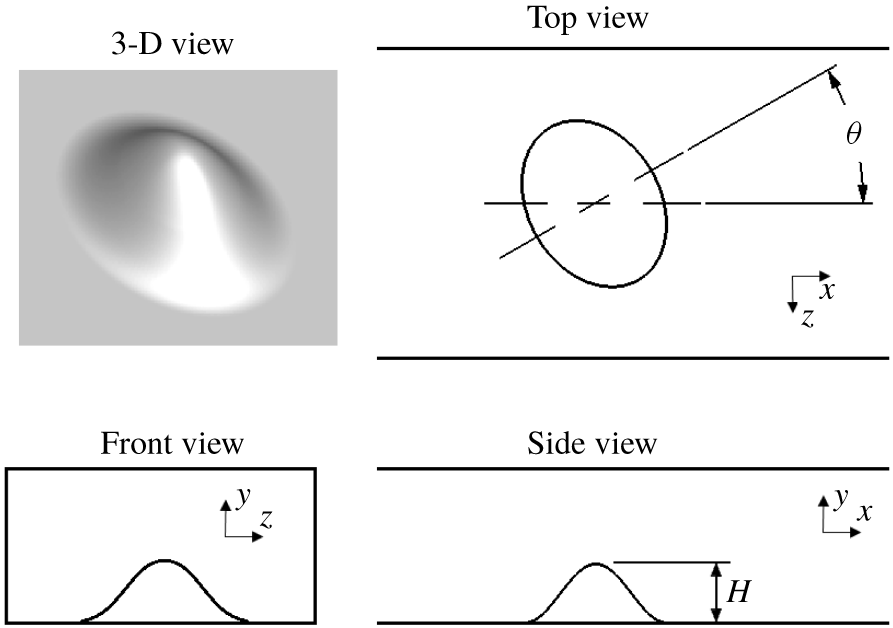
The flow configuration is a three-dimensional wall-mounted skewed bump on the bottom wall of a channel (figure 1) with Reynolds number of 16 000 (based on bump height), studied experimentally by Ching et al. (Reference Ching, Elkins and Eaton2018a,Reference Ching, Elkins and Eatonb). The bump has cosine cross-sections viewed from the side and elliptical cross-sections viewed from above with axis ratio of  $4/3$. The equation for the bump surface with respect to the bump angle
 $\unicode[STIX]{x1D703}$ is
 $$\begin{eqnarray}\displaystyle y_{S}=H\left[0.5+0.5\,\text{cos}\left(2\unicode[STIX]{x03C0}\sqrt{{\displaystyle \frac{x_{S}^{2}}{b^{2}}}+{\displaystyle \frac{z_{S}^{2}}{a^{2}}}}\right)\right]\quad \text{for }\frac{x_{S}^{2}}{b^{2}}+\frac{z_{S}^{2}}{a^{2}}<\frac{1}{4}, & & \displaystyle\end{eqnarray}$$
where  $x_{S}$ and
 $z_{S}$ are the rotated coordinates
 $$\begin{eqnarray}\displaystyle & \displaystyle x_{S}=x\,\text{cos}(\unicode[STIX]{x1D703})+z\,\text{sin}(\unicode[STIX]{x1D703}), & \displaystyle\end{eqnarray}$$
 $$\begin{eqnarray}\displaystyle & \displaystyle z_{S}=x\,\text{sin}(\unicode[STIX]{x1D703})-z\,\text{cos}(\unicode[STIX]{x1D703}), & \displaystyle\end{eqnarray}$$
with  $a=57~\text{mm}$,
 $b=42.75~\text{mm}$ and
 $H=19~\text{mm}$. The coordinate origin is on the bottom wall under the centre of the bump, and the bump angle is defined such that at
 $\unicode[STIX]{x1D703}=0^{\circ }$ the blockage area is largest. The bump surface is on the bottom wall of a
 $50~\text{mm}\times 100~\text{mm}$ cross-section rectangular channel with bulk velocity of
 $0.83~\text{m}~\text{s}^{-1}$, and the boundary layer thickness measured with the bump removed is
 $\unicode[STIX]{x1D6FF}_{99}=0.5H$ at the bump location, where
 $H$ is the bump height. Two simulations are run at bump angles of
 $10^{\circ }$ and
 $50^{\circ }$ with matching geometry and flow conditions to the experimental data from Ching et al. (Reference Ching, Elkins and Eaton2018a).
Schematic of bump geometry in the channel. 3-D, three-dimensional.

2.2 Large-eddy simulation details
The LES use the incompressible flow solver Vida, maintained by Cascade Technologies. Vida is a finite-volume solver with second-order spatial discretization and Adams–Bashforth time advancement, and solves the low-Mach Navier–Stokes equations using the method developed by Ham (Reference Ham2007). The LES are run with the Vreman subgrid-scale model (Vreman Reference Vreman2004), and the time-averaged ratio of subgrid-scale viscosity to laminar viscosity is less than 1.75 at every point in the domain.
The computational domain of each LES contains the entire channel cross-section and extends from  $10.3H$ upstream of the bump apex to
 $12H$ downstream. Each grid contains 80 million elements. The grids fully resolve the boundary layer on the bottom wall with
 $y^{+}$ less than one, but use the wall model developed by Cabot and Moin (Reference Cabot and Moin2000) on the top and side walls. There is no separation on the top or side walls, so wall models should be reasonably accurate on those walls. The grids have maximum spacing of
 $0.033H$ in the streamwise (
 $X$) and spanwise (
 $Z$) directions and
 $0.013H$ in the wall-normal (
 $Y$) direction. In regions close to the bump, the grids are refined in the streamwise and spanwise directions to a maximum spacing of
 $0.013H$. The time step is
 $5\times 10^{-4}~\text{s}$, corresponding to non-dimensional time
 $\unicode[STIX]{x0394}t~U_{bulk}/H=0.022$.
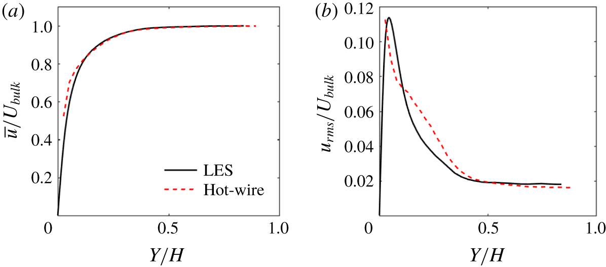
Mean streamwise velocity and r.m.s. velocity profiles were measured at  $X/H=-4$ with the bump removed from the channel (Ching et al. Reference Ching, Elkins and Eaton2018a). The experimental profiles were used to ensure that the LES match the experimental data at the same location. The free-stream turbulence intensity at
 $X/H=-4$ is 1.5 %. The LES generates inlet turbulence using the method of Xie and Castro (Reference Xie and Castro2008), which applies a two-dimensional filter to randomly generated numbers. The modification of Touber and Sandham (Reference Touber and Sandham2009) for generating normally distributed numbers is used to speed up the inflow generation. The filtered inlet velocities have an integral length scale of 0.003 m, which is approximately
 $1/3$ the boundary layer thickness at
 $X/H=-4$. To determine that the LES inlet conditions match the experimental data, a separate LES was run in a channel with identical cross-section but with the bump removed. Inlet conditions were specified such that profiles of mean and r.m.s. velocities had reasonable agreement with the experimental data at
 $X/H=-4$. Figure 2 shows profiles of the resulting mean streamwise velocity and r.m.s. streamwise velocity. The mean velocity profile has good agreement with the experimental data, but the r.m.s. velocity has differences. The differences are likely because the experimental boundary layer was tripped, but the LES did not model the boundary layer trip. The momentum thickness at
 $X/H=-4$ is
 $0.042H$ and the shape factor is 1.7. The boundary layer development section has a length of
 $12\unicode[STIX]{x1D6FF}$ between the inlet and
 $X/H=-4$, where
 $\unicode[STIX]{x1D6FF}$ is the boundary layer thickness at
 $X/H=-4$. The inlet conditions from the channel LES are used for both bump simulations.
(a) Mean streamwise velocity profile at  $X/H=-4$ with the bump removed. (b) Profile of r.m.s. streamwise velocity.

After initialization, the simulation is run for 2.5 s of simulation time (approximately five flow-through times) before recording statistics. Statistics are collected for 13.5 s of simulation time for the  $10^{\circ }$ bump LES, corresponding to
 $590H/U_{bulk}$ or approximately 70 shedding cycles. Statistics of the
 $50^{\circ }$ bump LES are collected for 8.5 s of simulation time, corresponding to approximately 50 shedding cycles.
3 Large-eddy simulation validation
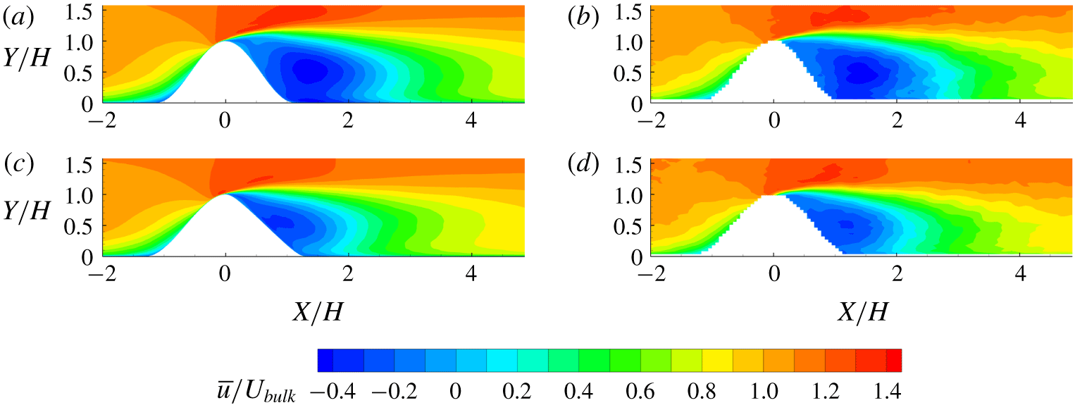
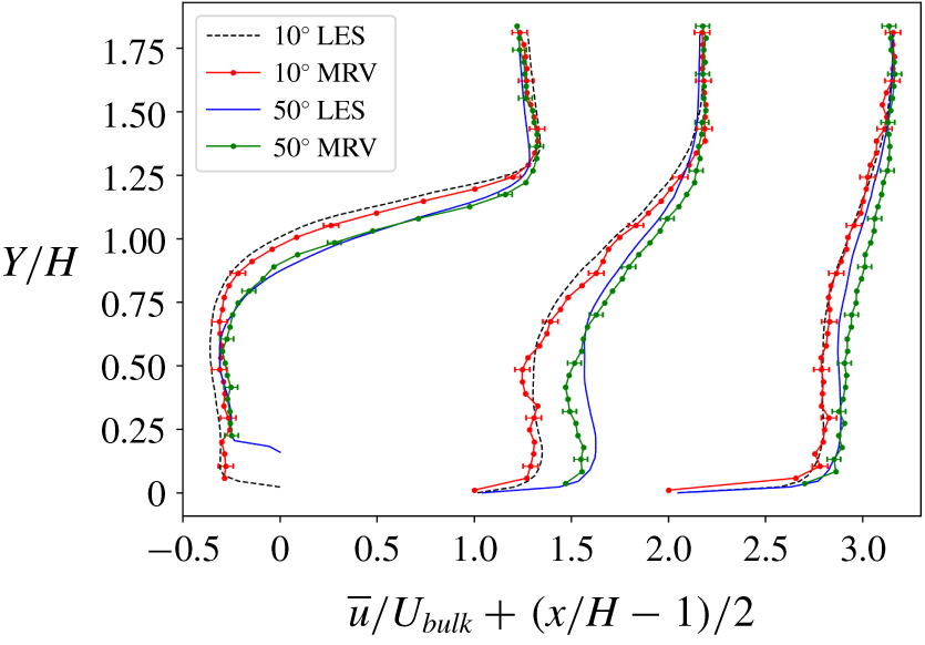
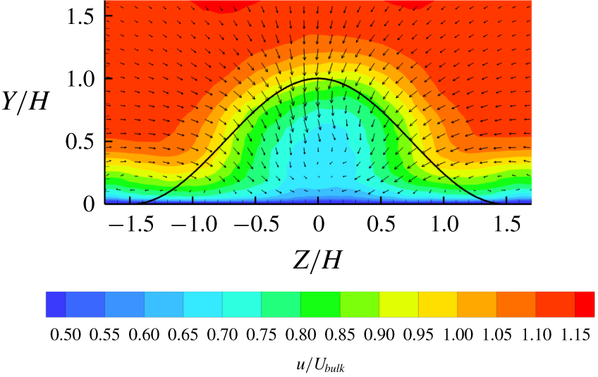
The LES are validated by comparison to mean velocity data in Ching et al. (Reference Ching, Elkins and Eaton2018a). Figure 3 shows good agreement between contours of streamwise velocity from the LES and experiments on the centreplane ( $Z=0$) at both bump angles. A more quantitative comparison is possible in figure 4, which shows centreline mean streamwise velocity profiles at three streamwise locations. Close agreement between simulation and experiment is found at all positions for the
 $10^{\circ }$ case. For the
 $50^{\circ }$ case, there is a measurable disagreement in the region at
 $X/H=3$. This could be a result of small differences in separation location. Generally, the simulations do a good job of capturing the significant differences between the
 $10^{\circ }$ and
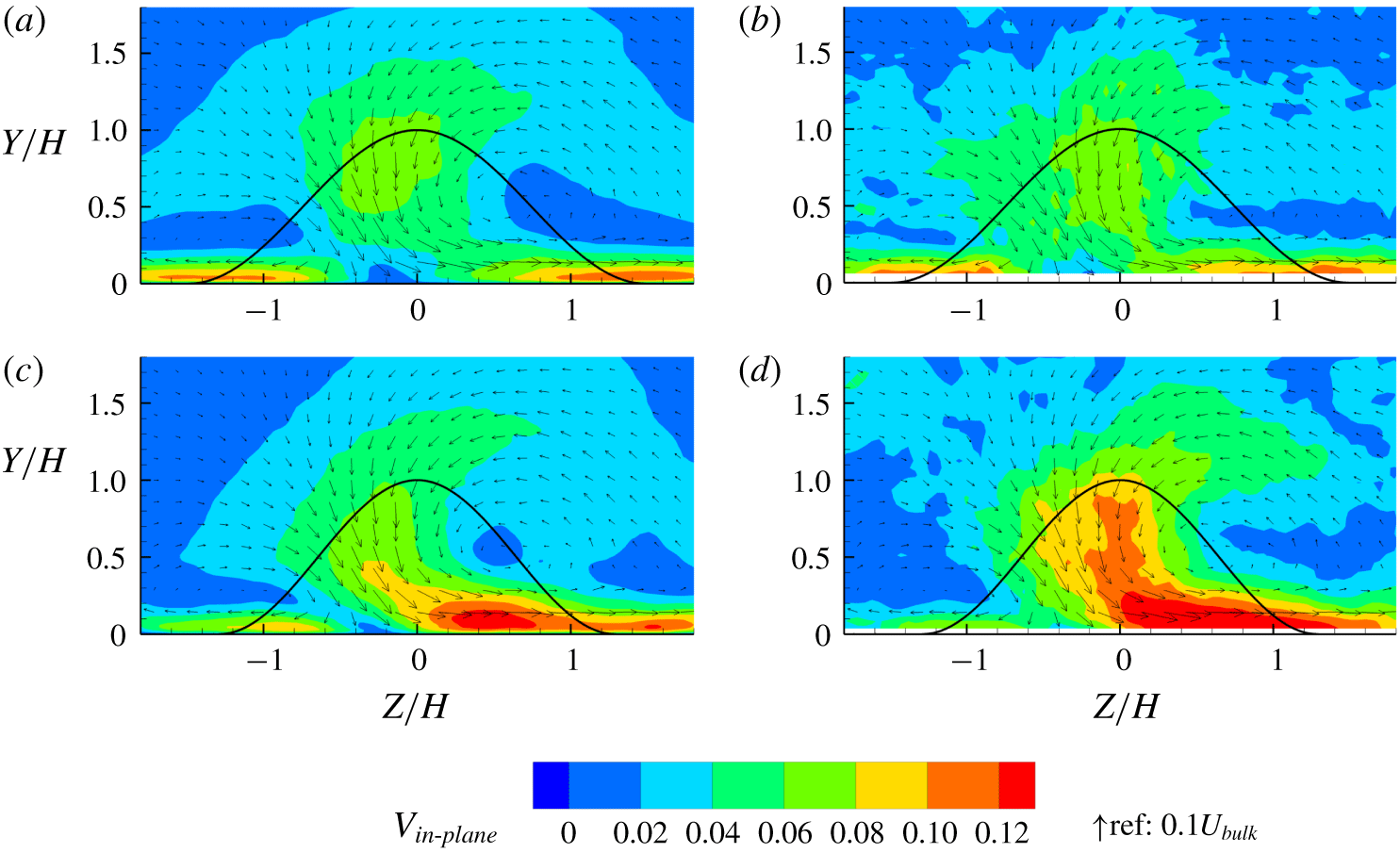
 $50^{\circ }$ cases. Figure 5 shows that the in-plane velocities at
 $X/H=6$ between experiment and LES have reasonably good agreement. The LES slightly underpredicts the strength of the secondary flow in the
 $50^{\circ }$ bump, but accurately predicts the location of the vortex centre.
(a) Centreplane streamwise velocity contours of  $10^{\circ }$ bump from LES; (b)
 $10^{\circ }$ bump experimental data from Ching et al. (Reference Ching, Elkins and Eaton2018a); (c)
 $50^{\circ }$ LES; (d)
 $50^{\circ }$ experiment.

Vertical profiles of streamwise velocity located at  $X/H=1$, 3 and 5 on the centreline,
 $Z/H=0$. The profile at
 $X/H=3$ is shifted on the horizontal axis by
 $1$ and the profile at
 $X/H=5$ is shifted by
 $2$. Uncertainties from Ching et al. (Reference Ching, Elkins and Eaton2018a) are plotted every fourth point on the experimental data.

(a) The  $10^{\circ }$ bump in-plane velocity magnitude contours with in-plane velocity vectors at
 $X/H=6$ from LES. The curve shows the bump profile projected on the plane. (b) The
 $10^{\circ }$ bump experiment of Ching et al. (Reference Ching, Elkins and Eaton2018a); (c)
 $50^{\circ }$ bump LES; (d)
 $50^{\circ }$ bump experiment.

The Strouhal number was identified experimentally in Ching et al. (Reference Ching, Elkins and Eaton2018b) using hot-wire data. The Strouhal number is defined for this case as
 $$\begin{eqnarray}\displaystyle St=\frac{f(A_{block})^{0.5}}{U_{bulk}}, & & \displaystyle\end{eqnarray}$$
where  $A_{block}$ is the blockage area,
 $U_{bulk}$ is the bulk velocity of
 $0.83~\text{m}~\text{s}^{-1}$ and
 $f$ is the shedding frequency. The Strouhal number is defined with the square root of blockage area as the length scale because the
 $50^{\circ }$ bump has a 13.2 % smaller blockage area than the
 $10^{\circ }$ bump, and objects with smaller blockage area generally have higher shedding frequencies. Table 1 shows the Strouhal number calculated from velocity power spectra in the wake between LES and experiments, with very close agreement. Overall, the experimental comparisons indicate that LES captures the true flow physics of the non-axisymmetric bump flow, so the results can be used to study the details of the quasi-periodic shedding cycle and its interactions with turbulence.
Strouhal number computed from LES and experiments of Ching et al. (Reference Ching, Elkins and Eaton2018b).

4 Results
4.1 Flow statistics
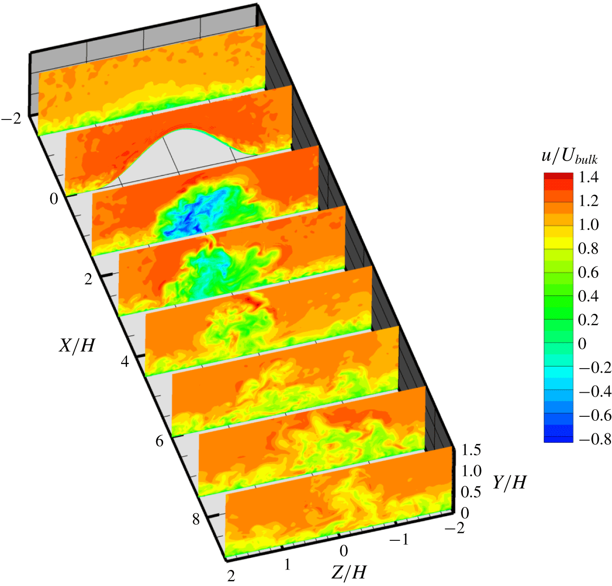
Figure 6 shows contours of instantaneous streamwise velocity at several planes from the  $10^{\circ }$ bump LES, showing that the flow in the wake is highly turbulent. For both bump angles, the flow separates near the top of the bump, creating a large recirculation zone in the wake, visible in figure 3. The main reversed-flow region extends to
 $X/H=2.4$ for the
 $10^{\circ }$ bump and
 $X/H=1.8$ for the
 $50^{\circ }$ bump, and the backflow is stronger in the
 $10^{\circ }$ case. In Ching et al. (Reference Ching, Elkins and Eaton2018a), it was found that the separation bubble volume changes significantly with bump angle. Although a smaller separation bubble volume is expected for angles with a smaller blockage area, the volume change was more than could be explained by a geometric scaling by blockage area. The wake deficit also decays faster for the
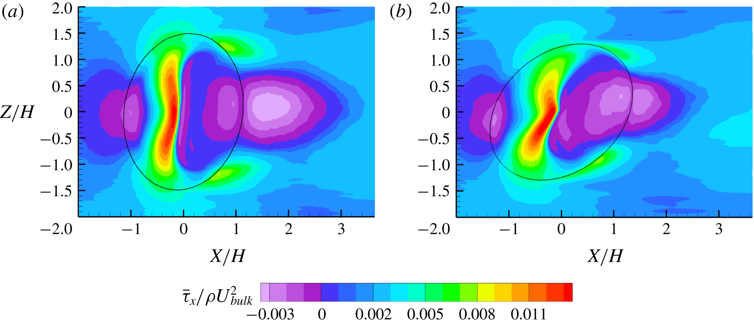
 $50^{\circ }$ bump. Both bumps also have a small upstream separation bubble due to the adverse pressure gradient as the boundary layer approaches the bump. The upstream separation bubble is very thin and the flow reattaches on the windward face of the bump. The reversed-flow region has negative streamwise wall shear stress, and figure 7 shows the extent of the upstream reversed-flow region near
 $X/H=-1$ for both bump angles. The upstream reversed-flow region is slightly larger in the
 $10^{\circ }$ bump case, but the difference is not large.
Contours of instantaneous streamwise velocity from the  $10^{\circ }$ bump LES. The planes shown are spaced at intervals of
 $1.5H$.

(a) Wall shear stress in  $X$ direction from
 $10^{\circ }$ bump LES. The edge of the bump is shown as a solid line. (b) Wall shear stress in
 $X$ direction from
 $50^{\circ }$ bump.

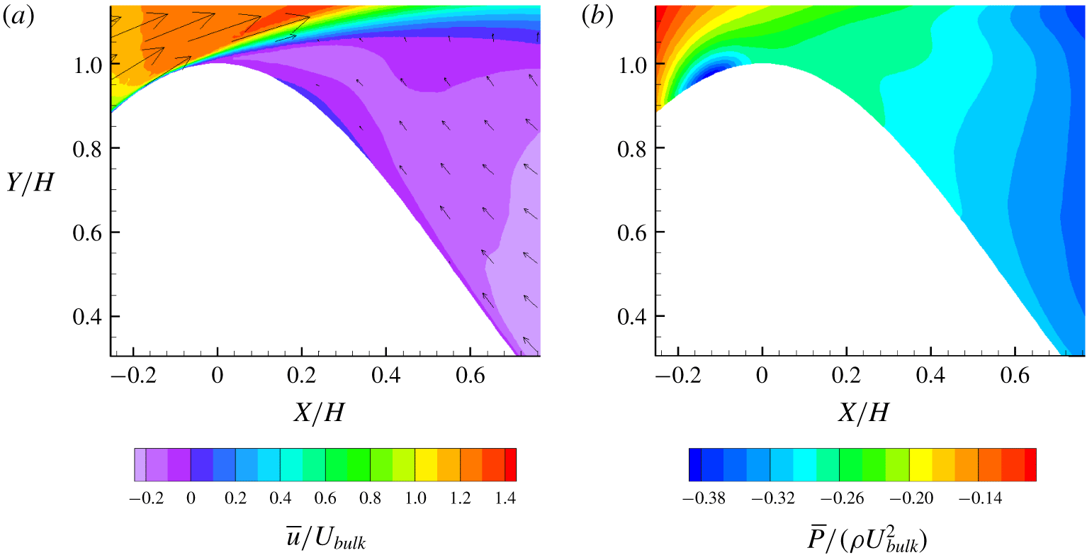
(a) Contours of  $10^{\circ }$ bump LES streamwise velocity and in-plane velocity vectors at
 $Z=0$ showing the secondary separation bubble. (b) Contours of mean pressure.

(a) Contours of  $10^{\circ }$ bump streamwise velocity with in-plane velocity vectors at
 $X/H=1.5$ from LES. The curve shows the bump profile projected on the plane. (b) The
 $50^{\circ }$ bump at
 $X/H=1.5$; (c)
 $10^{\circ }$ bump at
 $X/H=4$; (d)
 $50^{\circ }$ bump at
 $X/H=4$; (e)
 $10^{\circ }$ bump at
 $X/H=8$; (f)
 $50^{\circ }$ bump at
 $X/H=8$.

An interesting feature of the  $10^{\circ }$ bump is secondary separation in the main separation bubble. The reversed flow in the main separation bubble detaches from the surface as it sweeps up the leeward side of the bump, creating the secondary separation bubble visible as a blue patch just downstream of the bump apex in figure 8(a). The secondary separation bubble is very thin and does not significantly deflect the reversed flow. The wall shear stress in figure 7(a) shows the secondary separation bubble as a region of positive
 $\unicode[STIX]{x1D70F}_{x}$ between regions of negative
 $\unicode[STIX]{x1D70F}_{x}$. It extends the entire width of the primary separation bubble and joins with the downstream-moving flow at the sides of the bump. The secondary separation is not evident in the experimental data of Ching et al. (Reference Ching, Elkins and Eaton2018a) due to insufficient resolution near the wall. Figure 7(b) shows that no secondary separation exists in the
 $50^{\circ }$ case.
Secondary separation bubbles are known to exist in backward-facing steps due to Moffatt eddies in the corner, but are not typically seen in flows with smooth wall separation (Moffatt Reference Moffatt1964; Le et al. Reference Le, Moin and Kim1997). For secondary separation to exist, there must be an adverse pressure gradient along the direction of flow within the primary separation bubble. Figure 8(b) shows that the pressure is lower on the leeward side of the bump than near the top, so as the reversed flow moves up the bump surface, it encounters an adverse pressure gradient, leading to separation. Near the top, the pressure gradient reverses and reattaches the secondary separation bubble.
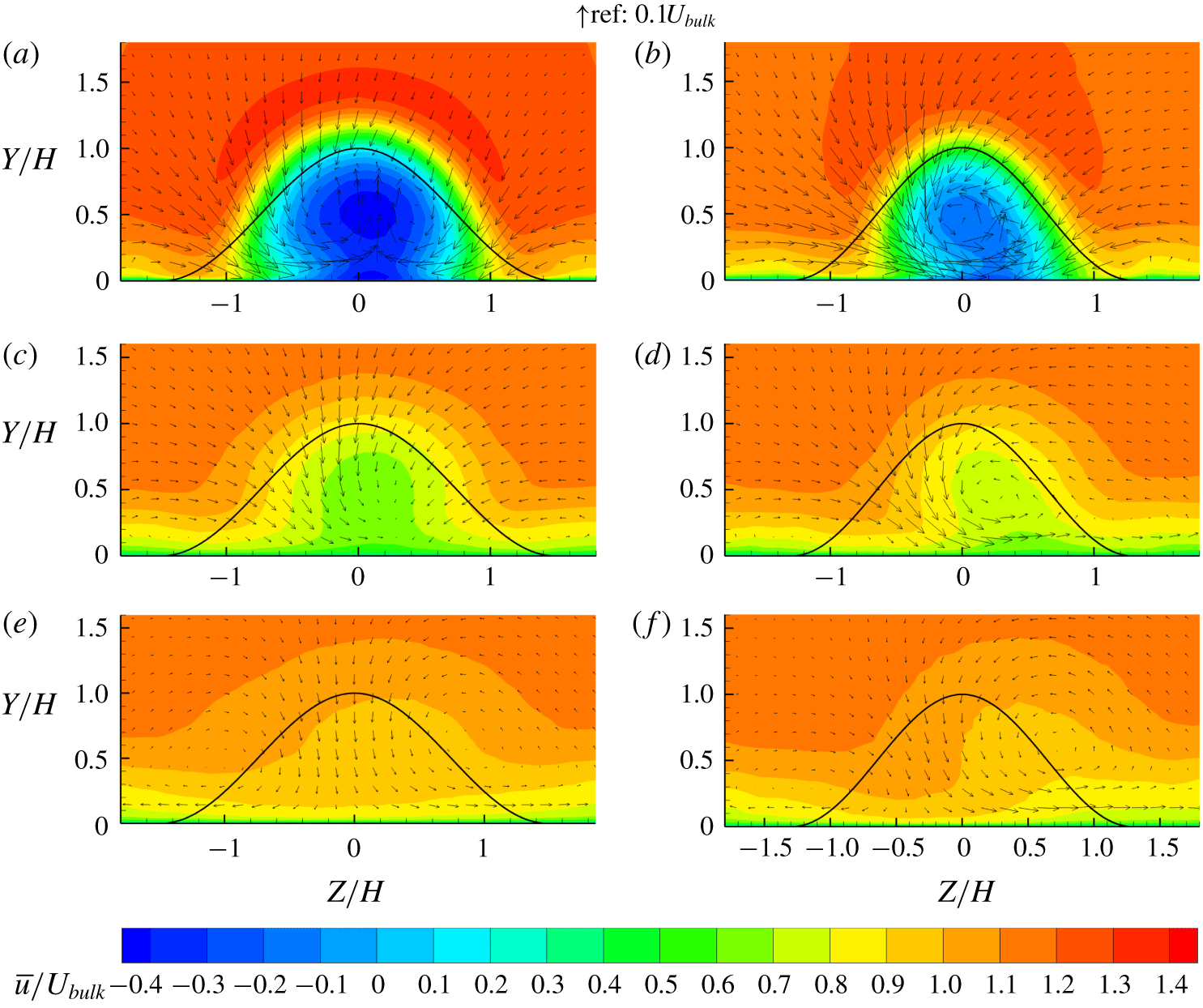
The mean flow fields show streamwise vortices in the wake. Figure 9 shows  $y{-}z$ planes at
 $X/H=1.5$,
 $X/H=4$ and
 $X/H=8$ for both bump angles. For the
 $10^{\circ }$ bump angle, the plane at
 $X/H=1.5$ shows a pair of common-up vortices in the separation bubble, while at
 $X/H=8$ there are instead weak common-down vortices, as was found in the experiments. Asymmetry in the
 $10^{\circ }$ case is most evident at
 $X/H=4$, where there is non-zero mean spanwise velocity on the centreline. The
 $50^{\circ }$ angle has a single counterclockwise vortex structure in the separation bubble that moves in the positive
 $Z$ direction as it advects downstream and is visible in all the
 $y{-}z$ planes. The dynamics of how the common-up vortex pair develops into a common-down pair can only be understood in the context of the quasi-periodic shedding cycle, and is explained in § 4.2.3.
Longitudinal vortices are observed in other wall-mounted flows, such as semi-ellipsoids (Hajimirzaie, Wojcik & Buchholz Reference Hajimirzaie, Wojcik and Buchholz2012), finite-length cylinders (Pattenden, Turnock & Zhang Reference Pattenden, Turnock and Zhang2005), pyramids (AbuOmar & Martinuzzi Reference AbuOmar and Martinuzzi2008) and vertical plates (Mason & Morton Reference Mason and Morton1987). For symmetric bodies, mean vertical velocity on the centreline in the near wake may be in either direction depending on the geometry and flow conditions. Vertical velocity in the direction away from the wall (commonly referred to as upwash) is indicative of common-up vorticity, and vice versa. Mason and Morton (Reference Mason and Morton1987) observed that generally common-down vortices are associated with thin boundary layers and tall obstacles, while common-up vortices are associated with thick boundary layers and wide obstacles. Hajimirzaie et al. (Reference Hajimirzaie, Wojcik and Buchholz2012) observed evidence of common-up vortices in the near wake and common-down vortices in the far wake of an semi-ellipsoid, similar to the vortices in the  $10^{\circ }$ bump case.
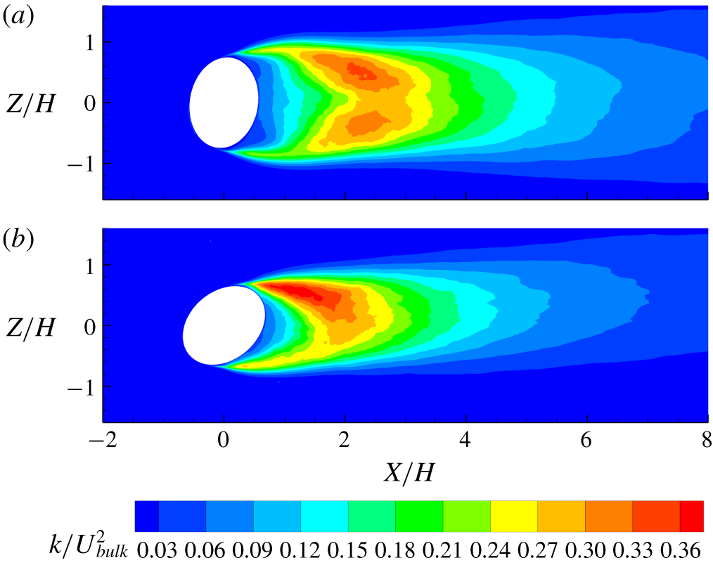
(a) The TKE contours at  $Y/H=0.5$ normalized by
 $U_{bulk}^{2}$ from the
 $10^{\circ }$ bump. (b) The
 $50^{\circ }$ bump TKE.

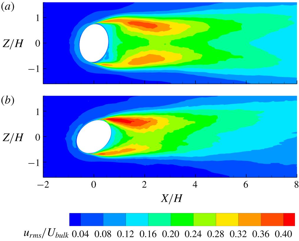
(a) Streamwise r.m.s. velocity contours at  $Y/H=0.5$ from
 $10^{\circ }$ bump normalized by
 $U_{bulk}$. (b) The
 $50^{\circ }$ bump streamwise r.m.s. velocity.

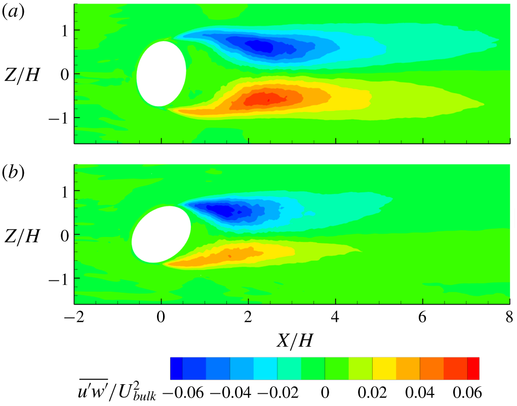
(a) The  $\overline{u^{\prime }w^{\prime }}$ contours at
 $Y/H=0.5$ from
 $10^{\circ }$ bump normalized by
 $U_{bulk}^{2}$. (b) The
 $50^{\circ }$ bump
 $\overline{u^{\prime }w^{\prime }}$.

Figure 10 shows TKE contours at  $Y/H=0.5$, where TKE is designated as
 $k$. While the TKE of the
 $10^{\circ }$ bump is nearly symmetric about the centreline, the
 $50^{\circ }$ bump has considerably higher TKE on the side with the trailing edge (positive
 $Z$). The TKE has a larger magnitude on the trailing-edge side of the
 $50^{\circ }$ bump than on either side of the
 $10^{\circ }$ bump, but the leading-edge side has significantly lower TKE than on the
 $10^{\circ }$ bump. This is not caused by buildup of boundary layer turbulence prior to separation, as the boundary layers have very low TKE in comparison to the wake. The higher fluctuations are likely caused by larger-scale motions associated with the quasi-periodic shedding cycle on that side.
The TKE asymmetry comes primarily from the streamwise components of velocity fluctuations  $u_{rms}$, shown in figure 11. Similar to TKE, the streamwise fluctuations on the trailing-edge side of the
 $50^{\circ }$ bump are stronger than for the
 $10^{\circ }$ bump. In the
 $10^{\circ }$ case, the streamwise fluctuations in the wake are highest in the shear layers near
 $X/H=2$ due to spanwise movements of the shear layer. The spanwise movements alternately bring high-speed free-stream fluid and low-speed fluid from the wake through the shear layer, causing high velocity fluctuations at fixed points. In figure 11(a) the fluctuations on the centreline far downstream of the separation bubble remain lower than at the sides despite high TKE that mixes fluid in the wake. Thus, spanwise profiles of
 $u_{rms}$ contain two peaks to the sides of the centre. Similar structures have been observed in the far wake of a circular cylinder (Matsumura & Antonia Reference Matsumura and Antonia1993; Kravchenko & Moin Reference Kravchenko and Moin2000; Parnaudeau et al. Reference Parnaudeau, Carlier, Heitz and Lamballais2008). It is shown in § 4.2.3 that the double peaks originate from motions of the quasi-periodic shedding cycle.
Figure 12 shows contours of the Reynolds shear stress streamwise–spanwise component  $\overline{u^{\prime }w^{\prime }}$ at
 $Y/H=0.5$. Positive streamwise fluctuations are correlated with spanwise fluctuations towards the centreline throughout most of the wake, suggesting that the wake has spanwise movements. The
 $10^{\circ }$ bump has significantly higher
 $\overline{u^{\prime }w^{\prime }}$ than the
 $50^{\circ }$ bump throughout the entire wake except on the trailing-edge side just after separation. The lower
 $\overline{u^{\prime }w^{\prime }}$ in the far wake of the
 $50^{\circ }$ case implies weaker wake movements.
4.2 Quasi-periodic cycle reconstruction
4.2.1 Spectral proper orthogonal decomposition
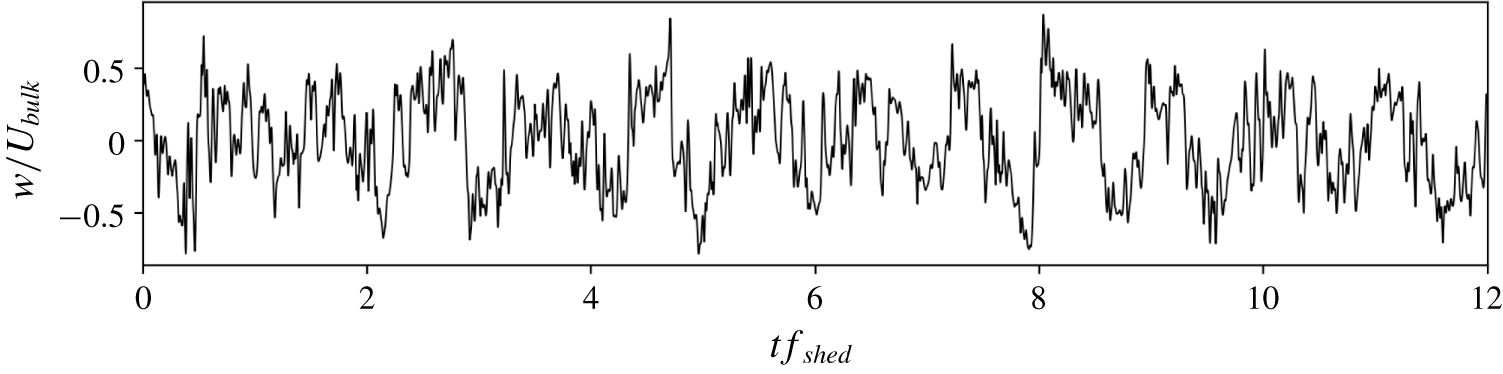
The Reynolds stresses suggest that the wake has spanwise movements which are likely a part of the quasi-periodic shedding cycle. Understanding the quasi-periodic vortex shedding cycle is critical to understanding the dynamics creating a common-up vortex pair in the separation bubble and a common-down pair downstream as well as the Reynolds stress distribution and wake recovery. Phase-averaging methods are difficult to use here due to the high broadband turbulence. For example, figure 13 shows a time series of spanwise velocity at  $(X/H,Y/H,Z/H)=(4.0,0.5,0)$, for which the power spectrum shows a strong peak at the shedding frequency. There are clear large-scale fluctuations, but identifying a specific phase is difficult.
Spanwise velocity time series at  $(X/H,Y/H,Z/H)=(4.0,0.5,0)$. Time is non-dimensionalized by the shedding frequency.

We use SPOD to calculate modes at the shedding frequency that describe the vortex shedding dynamics. SPOD is a model order reduction technique that identifies modes evolving coherently in space and time at distinct frequencies (Lumley Reference Lumley1970; Towne, Schmidt & Colonius Reference Towne, Schmidt and Colonius2018). The advantage of SPOD over proper orthogonal decomposition is that SPOD isolates dynamics at a single frequency and therefore ignores broadband turbulence at other frequencies. We use SPOD to reconstruct the vortex shedding cycle from modes at the shedding frequency.
SPOD finds modes  $\unicode[STIX]{x1D713}_{i}(x,f_{k})$ that are a function of space and operate at frequency
 $f_{k}$. The modes are calculated using the method described in Towne et al. (Reference Towne, Schmidt and Colonius2018) and summarized here. A time series of instantaneous flow snapshots are divided into
 $N_{w}$ fixed-length windows with 50 % overlap, each of length
 $T_{w}$. The data from each individual snapshot are arranged into a vector containing each velocity component at every point in the region of interest. The time Fourier transform is calculated on each window using a Hanning window with weights
 $w_{i}$, and the coefficients
 $\hat{q}_{k}^{(j)}$ at the chosen frequency
 $f_{k}$ are arranged into a matrix
 $$\begin{eqnarray}\displaystyle \hat{\unicode[STIX]{x1D64C}}_{f_{k}}=\sqrt{\frac{\unicode[STIX]{x0394}t}{sN_{w}}}[\hat{q}_{k}^{(1)},\hat{q}_{k}^{(2)},\ldots ,\hat{q}_{k}^{(N_{w})}], & & \displaystyle\end{eqnarray}$$
where  $s=\sum _{i=1}^{T_{w}}w_{i}^{2}$. The cross-spectral density tensor at frequency
 $f_{k}$ is
 $$\begin{eqnarray}\displaystyle \unicode[STIX]{x1D64E}_{f_{k}}=\hat{\unicode[STIX]{x1D64C}}_{f_{k}}\hat{\unicode[STIX]{x1D64C}}_{f_{k}}^{\ast }, & & \displaystyle\end{eqnarray}$$
where  $\hat{\unicode[STIX]{x1D64C}}_{f_{k}}^{\ast }$ is the complex conjugate transpose of
 $\hat{\unicode[STIX]{x1D64C}}_{f_{k}}$. The SPOD modes
 $\unicode[STIX]{x1D713}_{i}(x,f_{k})$ are the eigenvectors of
 $\unicode[STIX]{x1D64E}_{f_{k}}$. A useful property is that the eigenvalues of
 $\unicode[STIX]{x1D64E}_{f_{k}}$ tell how much energy is contained in each mode.
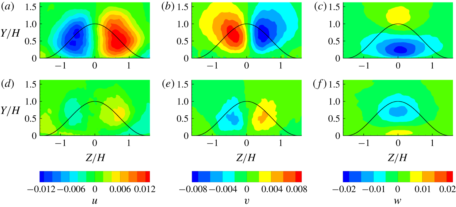
Each mode contains all three velocity components and has real and imaginary parts that are phase-shifted a quarter cycle. Figure 14 shows the first SPOD mode at the shedding frequency for the plane located at  $X/H=4$ in the wake of the
 $10^{\circ }$ bump. Because SPOD modes have arbitrary phase, the phase of the modes in figure 14 appear different from the SPOD modes in Ching et al. (Reference Ching, Elkins and Eaton2018b). SPOD modes operate at fixed frequency, so the modes show correlated fluctuations at the shedding frequency. The mode in figure 14 shows large-scale oscillations of each velocity component. The streamwise and wall-normal velocity components of the mode indicate spanwise oscillations, while the spanwise velocity appears to periodically sweep fluid across the centreplane near the wall.
(a) Real part of the  $u$ component from the first SPOD mode at
 $f_{shed}$. Modes are calculated from planes at
 $X/H=4$ on the
 $10^{\circ }$ bump. The curve shows the bump profile projected on the plane. (b) Imaginary part of
 $u$ component. (c) Real part of
 $v$ component. (d) Imaginary part of
 $v$ component. (e) Real part of
 $w$ component. (f) Imaginary part of
 $w$ component.

4.2.2 Reconstruction method
It is instructive to reconstruct the oscillating velocity field to understand how the quasi-periodic fluctuation modes average to the complex mean flow observed in experiments and LES. In particular, the mean wake contains longitudinal vortex structures and a region of lower streamwise velocity which likely have spatial movements over the shedding cycle. It is difficult to learn how they evolve just by examining SPOD modes, so we form a reduced-order model of the quasi-periodic cycle using the first SPOD mode at the shedding frequency. This method is similar to the reconstruction with proper orthogonal decomposition modes done by Van Oudheusden et al. (Reference Van Oudheusden, Scarano, Van Hinsberg and Watt2005). We apply SPOD only at the shedding frequency, so  $f_{k}$ corresponds to the shedding frequencies given in table 1. There are no significant peaks in power spectra at frequencies away from the shedding frequency peak, so it is sufficient that the reduced-order model contains only the shedding frequency.
The Fourier transform coefficients can be written as a linear combination of the SPOD modes. Using just one mode is equivalent to estimating the Fourier transform at  $f_{shed}$ as
 $$\begin{eqnarray}\displaystyle \hat{q}(x,f_{shed})=\mathop{\sum }_{i=1}^{N_{w}}a_{i}(f_{shed})\unicode[STIX]{x1D713}_{i}(x,f_{shed})\approx a_{1}(f_{shed})\unicode[STIX]{x1D713}_{1}(x,f_{shed}), & & \displaystyle\end{eqnarray}$$
where  $a_{i}(f_{shed})$ are coefficients of the modes. Reconstructing the cycle with just the first mode inherently assumes that the first SPOD mode represents shedding dynamics and the rest of the modes represent turbulence unrelated to shedding. Different SPOD modes can represent uncorrelated processes that occur at the same frequency, but the shedding cycle is highly correlated so it should be well represented by one mode.
Reconstructing the cycle using the SPOD mode at a single frequency implies that the power spectrum is a delta function at  $f_{shed}$. In reality, because the cycle is quasi-periodic, the power spectrum has a range of frequencies that correspond to shedding. To ensure that the reconstructed cycle contains the energy of the frequency band corresponding to shedding,
 $a_{i}(f_{shed})$ is replaced with
 $\sqrt{P_{rec}/2}$, where
 $P_{rec}$ is the power contained in the reconstructed cycle integrated in space and averaged in time. The method of calculating
 $P_{rec}$ is given below. Without this substitution, the reconstructed cycle would contain only a fraction of the energy due to shedding and would be dependent on the frequency resolution. The SPOD mode
 $\unicode[STIX]{x1D713}_{1}(x,f_{shed})$ has a unitary 2-norm, so specifying
 $P_{rec}$ is sufficient to ensure the reconstructed cycle contains the appropriate energy.
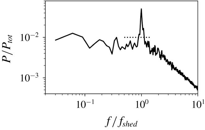
Power spectrum of velocity integrated over space and the three velocity components. The spectrum is normalized by total energy in the region of interest,  $P_{tot}$. The data are from the
 $10^{\circ }$ bump at
 $X/H=4$ within the region of interest
 $-1.8<Z/H<1.8$ and
 $0<Y/H<1.8$. The dotted line shows the average power in the range
 $0.5f_{shed}<f<1.5f_{shed}$.

The power in the shedding cycle is approximated by computing the power spectrum within the domain and integrating over a narrow frequency range near the shedding frequency. For example, figure 15 shows the power spectrum in the plane located at  $X/H=4$ of the
 $10^{\circ }$ bump within the region of interest
 $-1.8<Z/H<1.8$ and
 $0<Y/H<1.8$. There is a clear peak due to the quasi-periodic cycle, but the energy is spread over a range of frequencies. The shedding energy
 $P_{shed}$ is approximated as the integral of power over frequencies within the range
 $0.5f_{shed}<f<1.5f_{shed}$ and satisfying
 $P>\overline{P}_{r}$, where
 $\overline{P}_{r}$ is the mean of power over the frequencies
 $0.5f_{shed}<f<1.5f_{shed}$. These constraints ensure that only energy close to the shedding frequency and above broadband turbulence is considered. Table 2 shows the fraction of total energy associated with shedding for the planes in which the reconstructed cycle is shown.
All of the SPOD modes at  $f_{shed}$ together represent the energy at
 $f_{shed}$; thus,
 $P_{shed}$ must be multiplied by the fraction of energy in the first mode to approximate the power contained in the reconstructed cycle,
 $P_{rec}$. The eigenvalues of
 $S_{f_{shed}}$ have magnitude proportional to the energy in each mode, so the fraction of energy in the first mode is
 $\unicode[STIX]{x1D706}_{1}/\sum _{i}^{N_{w}}\unicode[STIX]{x1D706}_{i}$, where
 $\unicode[STIX]{x1D706}_{i}$ is the eigenvalue corresponding to mode
 $i$. Table 3 shows the fraction of energy in the first mode for each plane in which the reconstructed cycle is shown. The total energy of the reconstructed cycle is
 $$\begin{eqnarray}\displaystyle P_{rec}=\frac{\unicode[STIX]{x1D706}_{1}}{\displaystyle \mathop{\sum }_{i=1}^{N_{w}}\unicode[STIX]{x1D706}_{i}}P_{shed}. & & \displaystyle\end{eqnarray}$$
Since the reconstructed velocity is a real signal, its Fourier transform must contain delta functions at  $f_{shed}$ and
 $f_{-shed}$ that are complex conjugates of each other. The Fourier transform of the reconstructed cycle with the appropriate power is
 $$\begin{eqnarray}\displaystyle \hat{q}(x,f_{shed})=\sqrt{\frac{P_{rec}}{2}}(\unicode[STIX]{x1D713}_{1}(x,f_{shed})\unicode[STIX]{x1D6FF}_{f_{shed}}+\unicode[STIX]{x1D713}_{1}(x,f_{shed})^{\ast }\unicode[STIX]{x1D6FF}_{f_{-shed}}). & & \displaystyle\end{eqnarray}$$
Taking the inverse transform and adding the mean velocity yields the reconstructed cycle
 $$\begin{eqnarray}\displaystyle u_{r}(x,t)=\overline{u}(x)+\sqrt{2P_{rec}}(\unicode[STIX]{x1D713}_{1}^{(\text{R})}\text{cos}(2\unicode[STIX]{x03C0}f_{shed}t)-\unicode[STIX]{x1D713}_{1}^{(\text{I})}\text{sin}(2\unicode[STIX]{x03C0}f_{shed}t)), & & \displaystyle\end{eqnarray}$$
where  $\unicode[STIX]{x1D713}_{1}^{(\text{R})}$ and
 $\unicode[STIX]{x1D713}_{1}^{(\text{I})}$ are the real and imaginary parts of
 $\unicode[STIX]{x1D713}_{1}$ and
 $u_{r}(x,t)$ is the reconstructed cycle. In (4.6),
 $\overline{u}(x)$ and
 $u_{r}(x,t)$ contain all three velocity components at each point in the region of interest.
Fraction of energy associated with shedding,  $P_{shed}/P_{total}$.

Fraction of energy contained in the first SPOD mode,  $\unicode[STIX]{x1D706}_{1}/\sum _{i}\unicode[STIX]{x1D706}_{i}$.

This method assumes that only dynamics at the shedding frequency is important to the shedding cycle. In reality, is is possible that harmonics of the shedding frequency are also contained in the shedding cycle. However, the power spectrum of velocity integrated in space shown in figure 15 shows no peak at harmonics of the shedding cycle, which justifies reconstructing the cycle using a single mode at the shedding frequency.
4.2.3 Reconstructed cycle analysis
The cycle reconstruction was done in several  $y{-}z$ and
 $x{-}z$ planes. For all
 $y{-}z$ planes, the SPOD modes and reconstructed cycle are calculated in the region of interest
 $-1.8<Z/H<1.8$ and
 $0<Y/H<1.8$ to avoid including the top and sidewall boundary layers. In the
 $x{-}z$ plane, the region of interest is
 $-1.8<Z/H<1.8$ and
 $-2<X/H<12$. Inclusion of the top and sidewall boundary layers would add more broadband energy to the power spectrum, which makes identifying
 $P_{shed}$ more ambiguous. For the
 $10^{\circ }$ bump, SPOD was done on instantaneous velocities recorded every 10th time step, corresponding to a sampling rate 41 times the shedding frequency. For the
 $50^{\circ }$ bump, SPOD was done on the velocities every 14th time step, which is 24 times the shedding frequency. Each SPOD window contains 128 instantaneous flow snapshots. The SPOD modes are not sensitive to the window length or the precise frequency within 10 % of the shedding frequency.
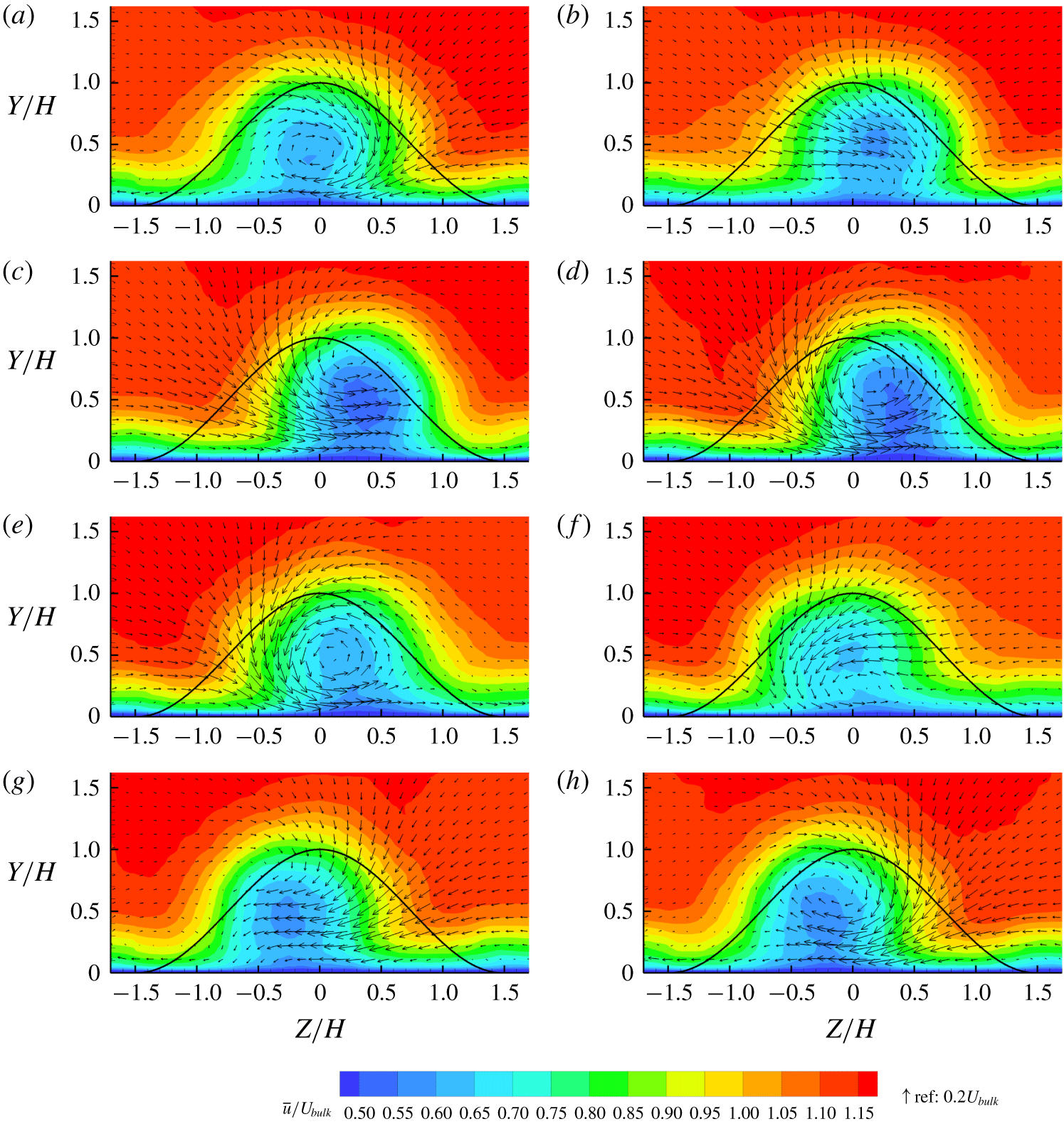
(a–h) The  $10^{\circ }$ bump reconstructed cycle using SPOD at
 $X/H=4$. Contours are streamwise velocity and vectors are in-plane velocity. Phases are at evenly spaced intervals of
 $1/8$ of the cycle. The curves show the bump profile projected on the plane.

Schematic of wake vortex dynamics.

(a–h) The  $50^{\circ }$ bump reconstructed cycle using SPOD at
 $X/H=4$. Contours are streamwise velocity and vectors are in-plane velocity. Phases are at evenly spaced intervals of
 $1/8$ of the cycle. The curves show the bump profile projected on the plane.

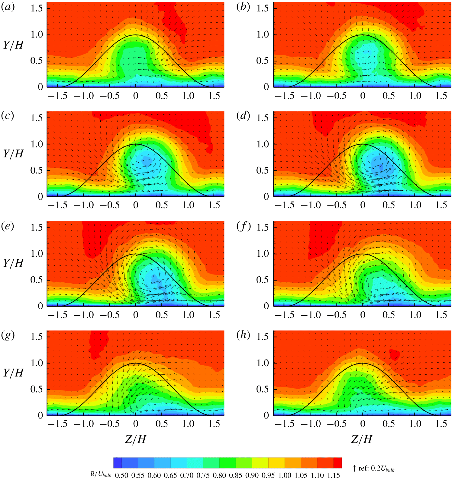
Figure 16 shows eight phases from the reconstructed cycle of the  $10^{\circ }$ bump at
 $X/H=4$, where subsequent images are spaced
 $1/8$ of the cycle apart. In figure 16(a–d), the streamwise velocity in the wake gradually decreases and the wake shifts from left to right. In figure 16(d–h), the streamwise velocity first increases, then decreases again and the wake shifts back to the left. The wake strength therefore ‘pulses’ twice each cycle and the wake oscillates in the spanwise direction. The in-plane velocities show a counterclockwise vortex developing in figure 16(c–e), then in figure 16(f–a) the counterclockwise vortex disappears and a clockwise vortex develops. The vortex roll-up coincides with the wake shifting to the side, and the movement is in the direction that would be induced by an image vortex (Marshall Reference Marshall2001). The image vortex of a clockwise vortex near the wall moves the vortex in the negative
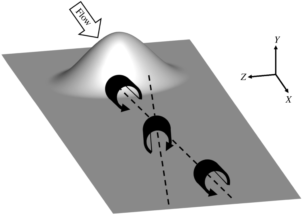
 $Z$ direction, and vice versa. While image vortices are derived from potential flow, it has been shown that longitudinal vortices near a wall have close agreement with the potential flow solution (Eibeck & Eaton Reference Eibeck and Eaton1987). The viscous effects typically are contained in a thin layer of vorticity very close to the wall, that typically has little effect on the vortex trajectory. Figure 17 is a schematic of the wake vortex dynamics, showing alternating vortices moving across the centreline as they are advected downstream. The reconstructed shedding cycle here is consistent with the experimental results from Ching et al. (Reference Ching, Elkins and Eaton2018b).
Although the  $10^{\circ }$ bump is only slightly asymmetric, there is asymmetry evident in the reconstructed cycle. As the streamwise velocity pulses twice over the cycle, it has troughs of low streamwise velocity when the wake is shifted furthest from the centreline in figure 16(d,h). The streamwise velocity is lower when the wake is on the trailing-edge side (figure 16d) than the leading-edge side (figure 16h). The asymmetry is also evident in the streamwise component of the SPOD mode (figure 14). The vortices do not show significant asymmetry at the
 $10^{\circ }$ angle.
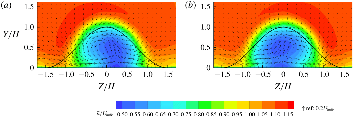
Figure 18 shows the reconstructed cycle from the  $50^{\circ }$ bump at the same location as for figure 16. Whereas in the
 $10^{\circ }$ bump the streamwise velocity in the wake ‘pulses’ twice each cycle, there is only one pulse in the
 $50^{\circ }$ bump. The wake deficit on the centreline also decays faster than in the
 $10^{\circ }$ bump. The
 $50^{\circ }$ bump wake oscillates in the spanwise direction, but the movements are considerably diminished in comparison to the
 $10^{\circ }$ bump. The
 $50^{\circ }$ bump does not have alternating opposite-sign vortices like the
 $10^{\circ }$ bump; the counterclockwise vortex in the
 $50^{\circ }$ bump has similar strength to the vortices in the
 $10^{\circ }$ bump, but the clockwise vortex never develops into a full vortex. Sensitivity to bump angle observed in the mean fields appears to be caused by a lack of a coherent clockwise vortex in the quasi-periodic cycle and weaker spanwise movements.
(a) The  $10^{\circ }$ bump reconstructed cycle using SPOD at
 $X/H=1.5$ showing phase when counterclockwise vortex is coherent. Contours are streamwise velocity and vectors are in-plane velocity. The curve shows the bump profile projected on the plane. (b) Phase when clockwise vortex is coherent.

Figure 19 shows two phases from the quasi-periodic cycle reconstruction at the plane  $X/H=1.5$ from the
 $10^{\circ }$ bump, which is within the separation bubble. The phases shown are chosen such that figure 19(a) is a phase when the counterclockwise vortex is coherent and figure 19(b) is half the cycle later when the clockwise vortex is coherent. Note that the clockwise vortex is right of the centreline and the counterclockwise vortex is left of the centreline. Downstream at
 $X/H=4$, figure 16 shows the vortices on opposite sides; the clockwise vortex is to the left of the centreline and the counterclockwise vortex is to the right of the centreline. The vortices therefore cross the centreline as they are advected downstream. This explains the observation of a common-up vortex pair in the mean fields within the separation bubble but a common-down pair downstream. The opposite-sign vortex pairs in the mean flow never exist in instantaneous field, but are a result of averaging over the quasi-periodic cycle. The clockwise vortices develop on the positive
 $Z$ side of the bump and the counterclockwise vortices on the opposite side, so they average to a common-up pair in the separation bubble. As the vortices move downstream, they cross the centreline as though pushed by image vortices. Downstream of the separation bubble, they average to a common-down pair.
(a–f) The  $10^{\circ }$ bump reconstructed cycle using SPOD at
 $Y/H=0.5$ showing contours of streamwise velocity and in-plane velocity streamlines. Phases are at evenly spaced intervals of
 $1/6$ of the cycle.

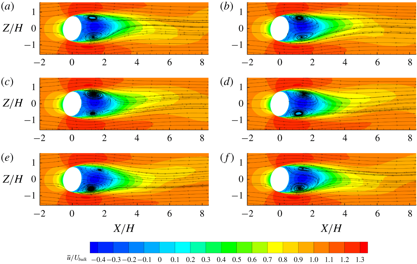
The quasi-periodic cycle reconstruction was done in an  $x{-}z$ plane at
 $Y/H=0.5$, with phases shown in figure 20 from the
 $10^{\circ }$ bump. Streamlines show wall-normal vortex structures in the separation bubble. However, downstream of the separation bubble, there is no evidence of wall-normal vortices in the reconstructed cycle or instantaneous fields. Due to the bump geometry and pressure gradients, boundary layer vorticity in the wall-normal direction is turned after detachment to create streamwise vorticity, which forms the large streamwise vortices (Ching et al. Reference Ching, Elkins and Eaton2018a).
The separation bubble and wake oscillate with spanwise motions as vortices are shed and carried downstream in figure 20. The streamwise velocity oscillations viewed in the  $Y/H=0.5$ plane are similar to shedding from a cylinder (Kravchenko & Moin Reference Kravchenko and Moin2000; Parnaudeau et al. Reference Parnaudeau, Carlier, Heitz and Lamballais2008). However, while a cylinder sheds vortices parallel to the cylinder axis, the bump flow sheds longitudinal vortices.
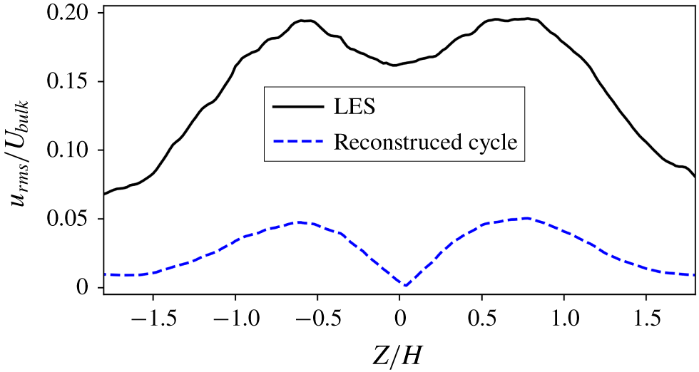
In figure 11 it was noted that streamwise velocity fluctuations far downstream have two peaks on either side of the centreline. Fluctuations due to the quasi-periodic shedding cycle explain the double peaks. The variance of the velocity in the reconstructed cycle can be derived from (4.6) as
 $$\begin{eqnarray}\displaystyle \overline{u_{r}^{\prime 2}}=P_{rec}[(\unicode[STIX]{x1D713}_{1}^{(\text{R})})^{2}+(\unicode[STIX]{x1D713}_{1}^{(\text{I})})^{2}]. & & \displaystyle\end{eqnarray}$$
Figure 21 shows spanwise profiles of streamwise velocity fluctuations at  $X/H=6$ and
 $Y/H=0.5$ from LES statistics and from the reconstructed cycle. The reconstructed cycle has lower
 $u_{rms}$ because it only accounts for fluctuations due to the shedding cycle whereas the LES statistics contain fluctuations at all frequencies. The difference between the two profiles is therefore due to small-scale turbulence. Both profiles have two peaks off the centreline, and the difference between
 $u_{rms}$ at the centreline and at the peaks is similar for the two profiles, suggesting that fluctuations from the quasi-periodic shedding cycle are responsible for the double peak. Matsumura and Antonia (Reference Matsumura and Antonia1993) similarly found that the double peak in streamwise fluctuations in the far wake of a cylinder was caused by the quasi-periodic shedding cycle. For a wall-mounted square cylinder, Bourgeois, Sattari & Martinuzzi (Reference Bourgeois, Sattari and Martinuzzi2011) observed that the coherent fluctuations due to the shedding cycle had a much larger contribution to the double peak than incoherent fluctuations due to small-scale turbulence.
Profile of streamwise r.m.s. velocity at  $X/H=6$ and
 $Y/H=0.5$ from LES statistics and from the reconstructed cycle.

4.2.4 Conditional averaging
The quasi-periodic cycle reconstruction ignores turbulence at scales outside the shedding frequency, so it does not show small-scale turbulent structures that are carried by the quasi-periodic shedding cycle. The separation bubble is highly turbulent and contains a wide range of scales, whereas the free stream has much lower turbulence. Fluid in the wake that was shed from the separation bubble would therefore be expected to have higher turbulence than free-stream fluid swept into the wake by quasi-periodic motions. We use conditional averaging to examine the relationship between small-scale turbulence and the quasi-periodic cycle.
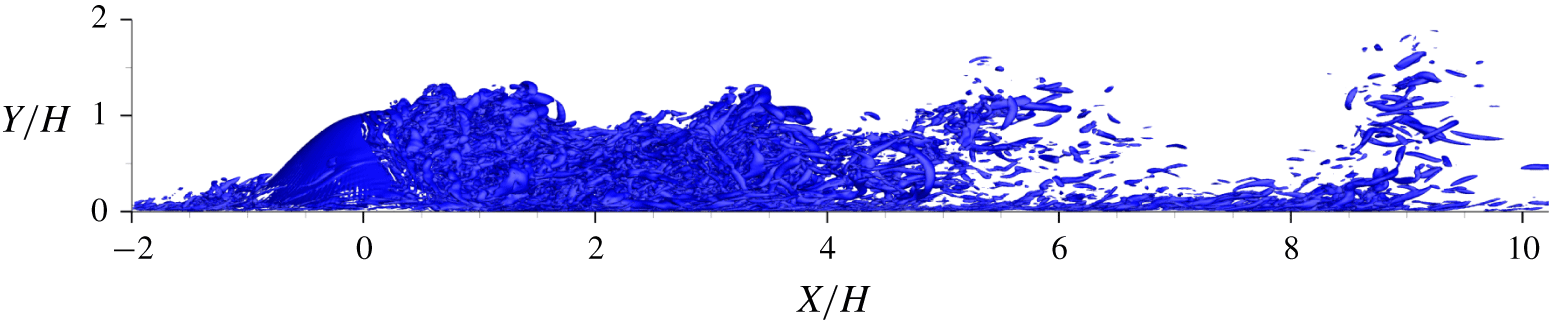
Instantaneous isosurfaces of  $Q$ criterion at
 $Q(H^{2}/U_{bulk}^{2})=20$ from the
 $50^{\circ }$ bump. Flow is left to right.

Figure 22 shows instantaneous isosurfaces of  $Q$ criterion (Hunt, Wray & Moin Reference Hunt, Wray and Moin1988) for a single snapshot from the
 $50^{\circ }$ bump. Regions of high turbulence appear between low-turbulence regions in the wake with a length scale of approximately
 $2H$ to
 $4H$. A distance of
 $4H$ at the bulk velocity corresponds to non-dimensional frequency of
 $0.25$, which is 1.6 times the shedding frequency (table 1). This suggests that the highly turbulent regions are related to the shedding cycle. The velocity in the wake is slower than the bulk velocity, so structures shed at the shedding frequency should appear closer together than if they were advected at free-stream velocity.
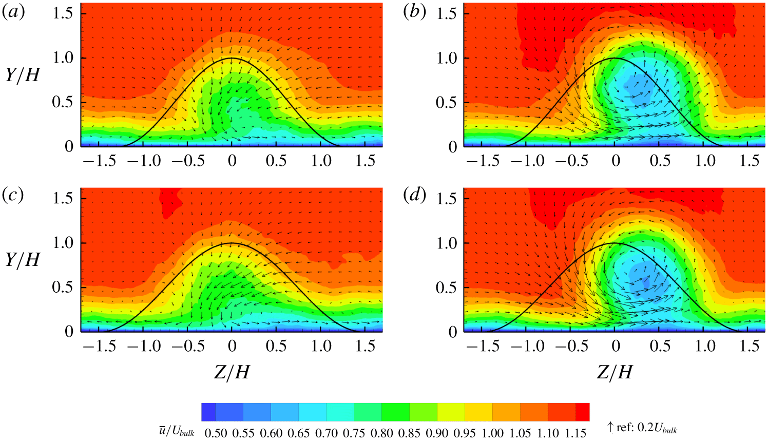
(a) Conditionally averaged flow snapshots at  $X/H=4$ with 20 % lowest condition (low turbulence) from
 $50^{\circ }$ bump. Contours are streamwise velocity and vectors are in-plane velocity. The curve shows the bump profile projected on the plane. (b) Conditionally averaged flow snapshots with 20 % highest condition (high turbulence). (c) Phase from reconstructed cycle with lowest least-squares difference from (a). (d) Phase from reconstructed cycle with lowest least-squares difference from (b).

Conditional averaging is used in the  $y{-}z$ plane located at
 $X/H=4$ to relate the turbulent regions to the reconstructed cycle. We use the squared streamwise vorticity,
 $\unicode[STIX]{x1D714}_{x}^{2}$, averaged over a spatial region of interest as a quantitative proxy for the instantaneous turbulence level in the wake (4.8):
 $$\begin{eqnarray}\displaystyle C_{1}=\frac{1}{A_{1}}\int _{A_{1}}\unicode[STIX]{x1D714}_{x}^{2}\,\text{d}A. & & \displaystyle\end{eqnarray}$$
The region of interest,  $A_{1}$, is chosen as
 $-1.8\leqslant Z/H\leqslant 1.8$ and
 $0\leqslant Y/H\leqslant 1.8$. Conditional averaging is done over the snapshots with the 20 % lowest
 $C_{1}$ on the
 $50^{\circ }$ bump in figure 23(a) and 20 % highest
 $C_{1}$ in figure 23(b). When turbulence is low, the wake has higher streamwise velocity and no vortex structure. When the turbulence is high, the wake has lower streamwise velocity, is shifted to the right and has a counterclockwise vortex. Figure 23(c,d) shows the two phases from the reconstructed cycle with the lowest least-squares difference from figure 23(a,b). The results from conditional averaging are strikingly similar to phases from the reconstructed cycle.
One potential concern is that the condition  $C_{1}$ is higher when the large vortex structure in figure 23(b,d) is present because the vortex structure has higher vorticity than the flow in figure 23(a,c). However, when the mean squared vorticity is calculated on the averaged fields in figure 23(a,b), the conditionally averaged low-turbulence field actually has higher
 $C_{1}$ than the high-turbulence field. While instantaneous snapshots have high vorticity magnitude wherever there is turbulence in the domain, the conditionally averaged fields have highest vorticity magnitude very close to the wall. The conditionally averaged low-turbulence field has slightly higher vorticity near the wall, leading to a higher
 $C_{1}$. However, the small-scale structures have much larger contribution to the condition. Therefore, the vortex structure has negligible contribution to
 $C_{1}$ in comparison to turbulence.
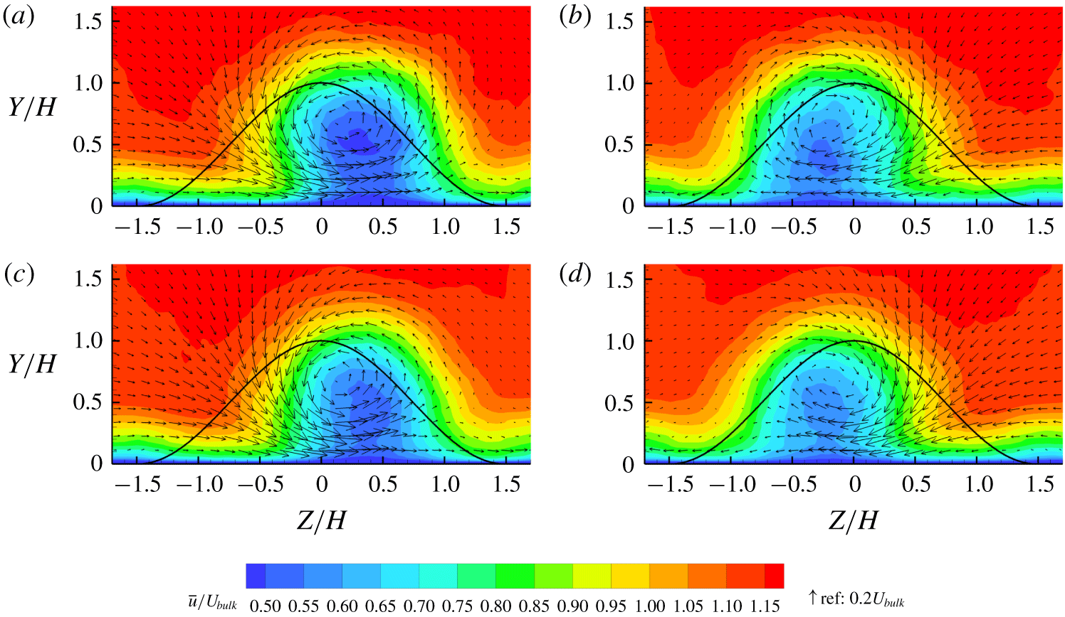
(a) Conditionally averaged flow snapshots at  $X/H=4$ with 40 % lowest
 $C_{2}$ from the set of snapshots with 30 % highest
 $C_{1}$ from
 $10^{\circ }$ bump. Contours are streamwise velocity and vectors are in-plane velocity. The curve shows the bump profile projected on the plane. (b) Conditionally averaged flow snapshots with 40 % highest
 $C_{2}$ from the set of snapshots with 30 % highest
 $C_{1}$. (c) Phase from reconstructed cycle with lowest least-squares difference from (a). (d) Phase from reconstructed cycle with lowest least-squares difference from (b).

Conditional averaging on the  $10^{\circ }$ bump is more complicated because the quasi-periodic cycle is nearly symmetric, so opposite-sign vortex structures have nearly the same turbulence and would be averaged together if the same method were used. To distinguish the clockwise and counterclockwise vortices, a second condition,
 $C_{2}$, defined in (4.9) is used to quantify whether the streamwise velocity in the wake is shifted to the right or left:
 $$\begin{eqnarray}\displaystyle C_{2}=\int _{A_{2}}u\,\text{d}A-\int _{A_{3}}u\,\text{d}A, & & \displaystyle\end{eqnarray}$$
where  $A_{2}$ is region of interest
 $0\leqslant Z/H\leqslant 0.5$ and
 $0\leqslant Y/H\leqslant 0.5$ and
 $A_{3}$ is region of interest
 $-0.5\leqslant Z/H\leqslant 0$ and
 $0\leqslant Y/H\leqslant 0.5$. Region of interest
 $A_{2}$ is to the right of the centreline and
 $A_{3}$ is to the left, so the subtraction in (4.9) is a measure of asymmetry. The method of conditional averaging for the
 $10^{\circ }$ bump is as follows. The 30 % of snapshots with highest
 $C_{1}$ form the set of high-turbulence snapshots. From that set, the 40 % of snapshots with the most negative
 $C_{2}$ are averaged and shown in figure 24(a), and the 40 % of snapshots with highest
 $C_{2}$ are averaged and shown in figure 24(b).
Figure 24(c,d) shows the two phases from the reconstructed cycle of the  $10^{\circ }$ bump with the lowest least-squares difference with the conditionally averaged images. Conditional averaging on high-turbulence snapshots of the
 $10^{\circ }$ bump leads to almost identical results to the reconstructed cycle. A counterclockwise vortex is observed when the wake is shifted to the right, and vice versa, meaning that the high turbulence level is observed at the specific phases where a strong longitudinal vortex is present. Figure 25 shows the result of conditional averaging the 30 % of snapshots with lowest
 $C_{1}$ (low turbulence). The wake streamwise velocity is significantly higher and no vortex structure is observed. There is no phase in the reconstructed cycle similar to the low-turbulence conditional average because the wake may be shifting right or left when the plane has low turbulence, and figure 25 is a result of averaging over both directions of movement.
Conditionally averaged flow snapshots with 30 % lowest  $C_{1}$ at
 $X/H=4$ from the
 $10^{\circ }$ bump. The curve shows the bump profile projected on the plane.

This method of conditional averaging using turbulence as the condition reveals that the vortices are associated with high turbulence. The similarity between velocity fields from conditional averaging and the reconstructed cycle implies a strong link between turbulence and the quasi-periodic cycle. As the bump sheds a vortex, high-turbulence fluid from the separation bubble is released into the wake and carried downstream with the vortex. Between vortex shedding events, free-stream fluid with low turbulence sweeps into the wake from the sides. The  $50^{\circ }$ bump sheds a single streamwise vortex per cycle while the
 $10^{\circ }$ bump sheds two vortices, so the
 $50^{\circ }$ bump releases a single burst of high turbulence while the
 $10^{\circ }$ bump releases two bursts per cycle. This undoubtedly contributes to the significantly higher TKE in the wake of the
 $10^{\circ }$ bump, seen in figure 10.
4.3 Surface pressures
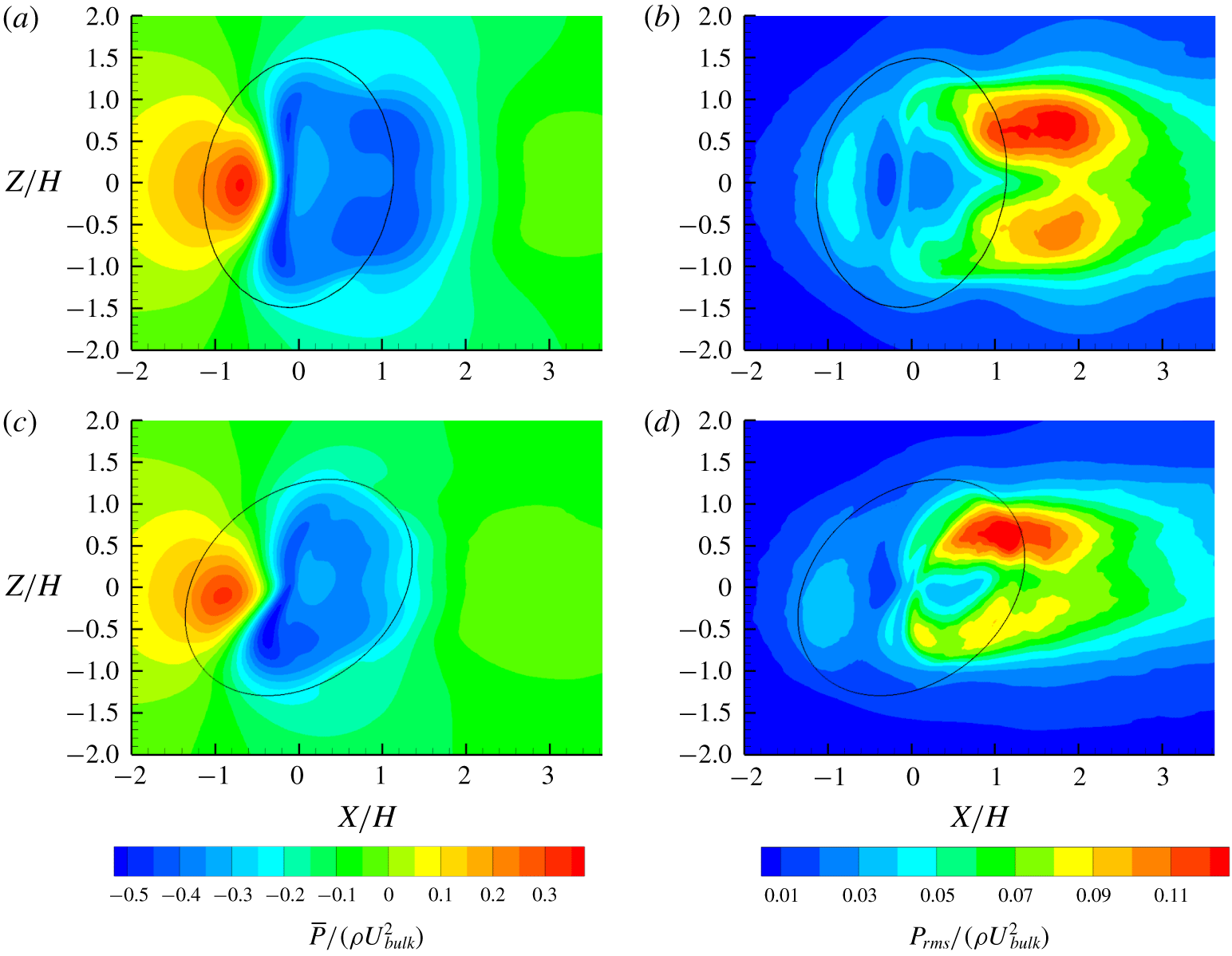
Surface pressure data from the simulations corroborate the findings about flow structures that were based on velocity fields. Figure 26(a) shows the surface mean pressure on the  $10^{\circ }$ bump. The pressures are referenced to the pressure at
 $(X/H,\,Z/H)=(-4,\,0)$ and normalized by
 $\unicode[STIX]{x1D70C}U_{bulk}^{2}$. Generally, the windward side of the bump has high pressure and the main separation bubble has low pressure, as would be expected for a bluff body. The mean pressure reaches a maximum on the upstream face near
 $X/H=-0.8$ and then decreases to a line of minimum pressure upstream of the apex. There is a short region of adverse pressure gradient upstream of separation. Slight asymmetry is observed in the pressure near separation; the pressure on the leading-edge side (negative
 $Z$) is slightly lower than on the trailing-edge side.
(a) Mean surface pressure on  $10^{\circ }$ bump from LES. The solid line shows the edge of the bump from (2.1). (b) The
 $10^{\circ }$ bump surface r.m.s. pressure; (c)
 $50^{\circ }$ bump mean surface pressure; (d)
 $50^{\circ }$ bump surface r.m.s. pressure.

Figure 26(b) shows the surface r.m.s. pressure. There are regions of high surface pressure fluctuations in the wake near  $X/H=1.8$ and
 $\pm Z/H=0.7$. The fluctuations are higher on the trailing-edge side, which is the side with higher velocity fluctuations (figure 10a). The high r.m.s. pressure is likely related to quasi-periodic motions. There is a region of high surface pressure fluctuations on the windward side of the bump near
 $X/H=-0.8$ coincident with reattachment of the upstream separation bubble (figure 7a). Fluctuations in the upstream separated region would cause movement of the pressure maximum, resulting in high r.m.s. pressure.
Figures 26(c) and 26(d) show the mean surface pressure and r.m.s. surface pressure on the  $50^{\circ }$ bump, respectively. On the windward side, both mean and r.m.s. pressures are slightly lower than in the
 $10^{\circ }$ bump. Near the separation location at the top of the bumps, the mean pressure on the leading-edge side of the
 $50^{\circ }$ bump is more negative than in the
 $10^{\circ }$ bump. In the wake, the region of low mean pressure is smaller in the
 $50^{\circ }$ bump, likely because the separation bubble is smaller. The r.m.s. pressures on the trailing-edge side in the wake are much stronger than on the leading-edge side.
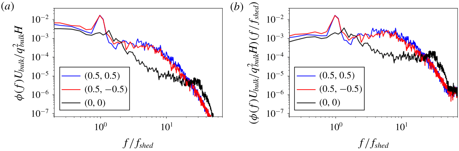
(a) Surface pressure spectra at  $(X/H,Z/H)=(0,0),(0.5,0.5)$ and
 $(0.5,-0.5)$ from the
 $10^{\circ }$ bump LES. Frequencies are non-dimensionalized by the experimental shedding frequency from table 1. The pressure spectra are non-dimensionalized by bulk velocity stagnation pressure
 $q_{bulk}$. (b) Pre-multiplied pressure spectra.

Surface pressures were recorded each time step at various positions on the  $10^{\circ }$ bump. Figure 27 shows pressure spectra at the bump apex and two points on the leeward side located at
 $(X/H,\,Z/H)=(0.5,\pm 0.5)$. The spectra at the points on the leeward side show distinct peaks aligned almost exactly with the experimentally measured shedding frequency (table 1). The spectrum at the apex does not show a peak at the shedding frequency and has less energy at low and midrange frequencies than the other two points. However, it has more energy at high frequencies, which we speculate is due to Kelvin–Helmholtz vortex roll-up of the separated shear layer.
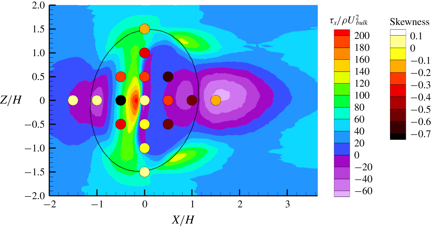
Skewness of surface pressure distribution at various points shown as coloured circles overlaid on streamwise wall shear stress. Data are from the  $10^{\circ }$ bump LES.

Figure 28 shows skewness of the wall pressure distribution at various locations plotted as coloured circles on top of a map of streamwise wall shear stress. The 95 % confidence interval on skewness is estimated to vary from 0.11 to 0.21. Although the confidence intervals are large due to the relatively short data records available, trends in skewness on the bump significantly exceed the uncertainty. On the windward side, the skewness is near zero at  $(X/H,\,Z/H)=(-1.5,\,0)$ and
 $(-1.0,\,0)$. The three points at
 $X/H=-0.5$ all have negatively skewed distributions, with the point on the centreline having the most negative skewness of
 $-0.8$. At
 $X/H=0$, the skewness varies between
 $-0.3$ and 0.1, and the asymmetry suggests that skewness depends strongly on the position relative to separation. The points with
 $X/H>0$ have negative skewness. In zero-pressure-gradient turbulent boundary layers, skewness is near zero. Negative skewness could be caused by the shape of oscillations associated with the quasi-periodic cycle, oscillations associated with flow separation or rare events unconnected with either the separation or the shedding cycle.
The two points at  $(X/H,Z/H)=(0.5,0.5)$ and
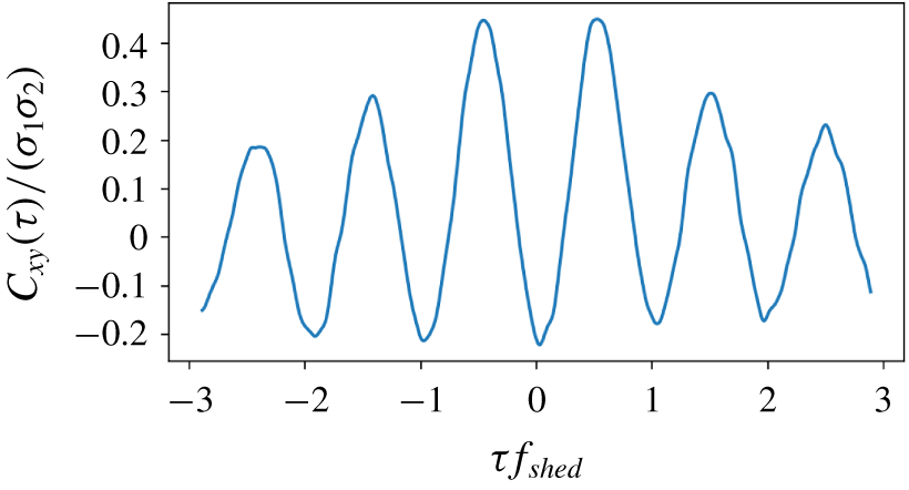
 $(0.5,-0.5)$ have very similar spectra and strong peaks at the shedding frequency in figure 27, so it is assumed that they have very similar pressure signals. The cross-correlation of the pressure signals at the two points is shown in figure 29. The cross-correlation with zero time shift is negative because the wake oscillates with spanwise motions. However, the minimum value is
 $-0.22$ at zero time shift while the maximum is 0.45 with a shift of
 $0.5/f_{shed}$. This disparity indicates that pressure peaks and valleys have different magnitudes, most likely due to the occurrence of a strong longitudinal vortex over the measurement point. Negative skewness implies that the negative peaks are larger than the positive ones, and positive fluctuations occur for a larger fraction of the time. This shows that the surface pressure fluctuations induced by the quasi-periodic cycle at those points have a larger negative peak than positive peak.
Cross-correlation of surface pressure at  $(X/H,Z/H)=(0.5,0.5)$ and
 $(0.5,-0.5)$ of the
 $10^{\circ }$ bump.

5 Conclusions
Wall-resolved LES of a skewed, wall-mounted, three-dimensional bump are used to examine wake dynamics at bump angles of  $10^{\circ }$ and
 $50^{\circ }$. The simulations reveal the presence of secondary separation with forward flow in the main separation bubble for the
 $10^{\circ }$ bump. In the mean velocity fields, the
 $10^{\circ }$ bump has a common-up longitudinal vortex pair in the separation bubble but a common-down pair further downstream. The
 $50^{\circ }$ bump has a single dominant longitudinal vortex existing through the entire wake. Temporal features of the flow, most notably a quasi-periodic wake shedding cycle, agree closely with experimental results presented by Ching et al. (Reference Ching, Elkins and Eaton2018b). The LES results allow a more detailed look at the temporal features than was possible using the experiments.
Understanding the quasi-periodic cycle is critical to explaining mean flow fields, turbulence and surface pressures in these flows. Although the shedding cycle contains only a small fraction of the TKE (table 2), it has a strong influence on the flow. The mean vortex structures in the bump wake and their sensitivity to flow angle, the Reynolds stress distributions, the release of broadband turbulence from the separation bubble and the surface pressure fluctuations in the separation bubble are all affected by the quasi-periodic cycle.
The shedding cycle occurs over a narrow frequency range and is somewhat similar to a Karman vortex street except that alternating-sign longitudinal vortices are shed from the two sides of the bump. SPOD at the bump shedding frequency is used to identify oscillation modes, and a reconstructed cycle is constructed from the SPOD modes in several planes. The reconstructed cycle ignores broadband turbulence and assumes all energy is at the shedding frequency, giving an ‘average’ shedding cycle. The reconstructed cycle of the  $10^{\circ }$ bump shows that the streamwise velocity in the wake pulses twice per cycle, the wake has spanwise oscillations and opposite-sign vortices alternately roll through the wake. The
 $50^{\circ }$ bump wake has less movement over the cycle; the streamwise velocity pulses only once and only a single vortex is evident in the wake. The vortices move across the centreline as they are advected downstream, which explains why the mean velocity of the
 $10^{\circ }$ bump has a common-up pair in the separation bubble but a common-down pair further downstream. Near the bump, the opposite-sign vortices of the quasi-periodic cycle average to a common-up pair, but after they cross the centreline they average to a common-down pair. We believe this may be a common feature of separated flows over three-dimensional surface-mounted obstacles. Nearly symmetric bodies producing little sideforce will produce alternating longitudinal vortices in the wake. By contrast, asymmetric bodies producing significant sideforce will produce very asymmetric vortex structures.
The wake has alternating regions of high and low turbulence that are advected downstream and produce a distinctive signature in the mean Reynolds stress distributions. Conditional averaging identifies that the regions of high turbulence are associated with low streamwise velocity and a vortex structure in the wake. In each cycle, the  $50^{\circ }$ bump releases one burst of turbulence, while the
 $10^{\circ }$ bump releases two. The conditionally averaged velocities are very similar to phases from the reconstructed cycle, which shows that turbulence is strongly linked to vortex shedding.
There are strong cycle-to-cycle variations evident in the data, and potential future work examining them could be interesting. The current simulations are run for approximately 50 to 70 shedding cycles, which is not enough to collect converged statistics on cycle-to-cycle variations. A simulation would need to be run for much longer to analyse those variations.
Surface pressure distributions on the  $10^{\circ }$ bump have negative skewness in the separation bubble and in a region on the windward face. Surface pressure fluctuations caused by the quasi-periodic cycle are found to contribute to the negative skewness by having a larger negative peak than positive peak.
Many three-dimensional separated flows exhibit complicated mean flow and turbulence structures that often include dominant longitudinal vortices. Quasi-periodic shedding of longitudinal vortices may be important in many of these flows and should be examined in future research.
Acknowledgements
The authors gratefully acknowledge financial support from the Office of Naval Research grant no. N00014-15-1-2352 and from the Achievement Rewards for College Students (ARCS) foundation. We are also grateful to Cascade Technologies for providing the LES code Vida and Dr A. Banko for his comments on this paper.