1 Introduction
High-resolution observational datasets in atmosphere and ocean fluid dynamics are usually very restricted in their spatial coverage; they are often confined to either an essentially one-dimensional horizontal ship or aircraft track, or to a narrow sweep of a remote-sensing instrument. Methods that can extract the maximum of information from such one-dimensional measurements are therefore crucial, especially as recent progress in measurement and modelling techniques provides a growing window into the ‘submesoscale’ wave–vortex jigsaw puzzle that is typical for three-dimensional stratified rotating fluids (e.g. McIntyre Reference McIntyre2008).
In this connection, a new wave–vortex decomposition method for one-dimensional power spectra obtained from horizontal ship and aircraft-track data was recently developed in Bühler, Callies & Ferrari (Reference Bühler, Callies and Ferrari2014), hereafter BCF14, and Callies, Ferrari & Bühler (Reference Callies, Ferrari and Bühler2014). The first step of the new method takes as input the power spectra of the horizontal velocity field measured along the track and performs an exact Helmholtz decomposition of these spectra into their rotational and divergent components. Here we follow standard usage, whereby the rotational component is horizontally non-divergent and described by a stream function
 $\unicode[STIX]{x1D713}$
whilst the divergent component is horizontally irrotational and described by a flow potential
 $\unicode[STIX]{x1D719}$
. The relative magnitude of these spectral components already allows some deductions about the flow characteristics at various scales to be made, but rather more can be said. Indeed, in a second step an energy equipartition result from linear wave theory is utilized to estimate the wave energy spectrum of hydrostatic inertia–gravity waves solely based on the divergent part of the horizontal kinetic energy spectrum computed in the first step. This predicts the wave energy spectrum entirely from the observed horizontal velocity field along one-dimensional measurement tracks.
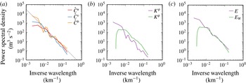
If buoyancy is also measured, then the total observed flow energy is available, and hence the difference between the observed total energy and the predicted wave energy provides an estimate of the energy contained in the vortical, quasi-geostrophic part of the horizontal motion. Comparison of the wave and the vortex energy levels then gives a useful tool with which to judge the physical nature of the measured flow field. The workings of the BCF14 method are illustrated in figure 1.
Illustration of the wave–vortex decomposition method from BCF14. (a) Observed horizontal velocity and buoyancy spectra at 200 m depth in the eastern subtropical North Pacific. (b) Helmholtz decomposition of the kinetic energy into rotational and divergent components
 $K^{\unicode[STIX]{x1D713}}$
and
 $K^{\unicode[STIX]{x1D719}}$
. (c) Observed total energy spectrum
 $E$
versus diagnosed wave energy spectrum
 $E_{W}$
, showing clearly that the flow is dominated by waves at scales below 100 km. This is not obvious from the raw data on the left.

The original method was developed for hydrostatic flows but its extension to non-hydrostatic flows is straightforward and allows application of the new method to high-resolution data in which the vertical velocity is measured as well (e.g. Zhang et al. Reference Zhang, Wei, Zhang, Bowman, Pan, Atlas and Wofsy2015; Callies, Bühler & Ferrari Reference Callies, Bühler and Ferrari2016). Overall, the new method is very easy to use and quite broadly applicable in the field (e.g. Balwada, LaCasce & Speer Reference Balwada, LaCasce and Speer2016; Bierdel et al. Reference Bierdel, Snyder, Park and Skamarock2016; Rocha et al. Reference Rocha, Chereskin, Gille and Menemenlis2016). We note in passing that the method could also be useful for a simple and computationally cheap local analysis of data from high-resolution numerical simulations.
Of course, the BCF14 method relies on a set of simplifying assumptions about the statistical flow structure and about the measurements themselves, which are assumed to occur at a fixed altitude and time. Specifically, for the Helmholtz decomposition step it is assumed that the flow is statistically homogeneous and isotropic in the horizontal plane and that the stream function and the potential are uncorrelated (the precise condition is (3.2) below). For the subsequent wave–vortex decomposition step it is furthermore assumed that the flow is stationary in time and also homogeneous in the vertical direction, which allows the linear wave field to be treated as a superposition of uncorrelated plane waves. Removing any of these assumptions would make the method more widely applicable and would allow to extract more information from the available datasets.
The present paper proposes an extension of this method that retains horizontal homogeneity, but allows for horizontal anisotropy. This is of obvious relevance to real atmosphere and ocean flows, where both the vortical flow and the wave field may exhibit pronounced anisotropies, especially at larger scales. For example, the vortical flow might exhibit strong directional currents such as the Gulf Stream, and the local internal wave field might be predominantly directed away from localized source regions such as prominent topography features exemplified by the Hawaiian ridge (e.g. Merrifield, Holloway & Johnston Reference Merrifield, Holloway and Johnston2001). Anisotropy is easily detected in data, though it is often ignored. For example, if
 $(u,v)$
are the horizontal velocity components such that
 $u$
is the longitudinal velocity aligned with the measurement track and
 $v$
is the transverse velocity at right angles to it, then isotropy implies that
 $$\begin{eqnarray}\mathbb{E}[u^{2}-v^{2}]=0\quad \text{and}\quad \mathbb{E}[uv]=0\end{eqnarray}$$
both hold. Here
 $\mathbb{E}$
denotes taking the expected value over the distribution of the velocity field, and a non-zero observed value in either of these two expectations would be sufficient to indicate the occurrence of anisotropy (e.g. Stewart et al.
Reference Stewart, Spence, Waterman, Le Sommer, Molines, Lilly and England2015).
However, it is important to note at the outset that any attempt to allow for anisotropic flow features in the analysis of one-dimensional power spectra must necessarily restrict to some constrained form of anisotropy, and cannot possibly treat the general case. This is for the following reason: the fundamental objects that describe the statistical flow structure are the horizontal two-point correlation functions for the underlying stream function and velocity potential. For example,
 $$\begin{eqnarray}C^{\unicode[STIX]{x1D713}}(x,y)=\mathbb{E}[\unicode[STIX]{x1D713}(x_{0},y_{0})\unicode[STIX]{x1D713}(x_{0}+x,y_{0}+y)]\end{eqnarray}$$
is the two-point correlation function for the stream function
 $\unicode[STIX]{x1D713}$
and its horizontal Fourier transform
 ${\hat{C}}^{\unicode[STIX]{x1D713}}(k,l)$
is the corresponding power spectrum (detailed definitions are given in the next section). Here
 $C^{\unicode[STIX]{x1D713}}$
does not depend on
 $(x_{0},y_{0})$
by the assumption of homogeneity and if the measurement track is aligned with
 $x$
then only the one-dimensional trace along
 $y=0$
of these functions is available.
In the isotropic case
 $C^{\unicode[STIX]{x1D713}}$
depends only on a single variable, which is the distance
 $r=\sqrt{x^{2}+y^{2}}$
between the two points. Such a function of a single variable can in principle be deduced from suitable observations of one-dimensional correlation functions along the track
 $y=0$
. On the other hand, in the general anisotropic case
 $C^{\unicode[STIX]{x1D713}}$
depends on the two variables
 $(x,y)$
and a general function of two variables cannot be deduced from one-dimensional measurements taken in a single direction. In other words, further restrictions must now be made on the possible form of the correlation functions. This is a common problem when fitting multi-dimensional power spectra to lower-dimensional data, and some form of tractable parametric anisotropy based on physical intuition is usually prescribed (e.g. Wortham, Callies & Scharffenberg Reference Wortham, Callies and Scharffenberg2014; Wortham & Wunsch Reference Wortham and Wunsch2014).
We are not aware of a systematic or optimal approach to this problem, so we followed our intuition to look for a simple and mathematically consistent form of anisotropy that is relevant to the physical situation at hand. Specifically, we took our cue from the relationships between the correlation functions of the horizontal velocity components
 $(u,v)$
and of the stream function
 $\unicode[STIX]{x1D713}$
and potential
 $\unicode[STIX]{x1D719}$
. As
 $u=-\unicode[STIX]{x1D713}_{y}+\unicode[STIX]{x1D719}_{x}$
it follows that
 $$\begin{eqnarray}C^{u}(x,y)=-\frac{\unicode[STIX]{x2202}^{2}}{\unicode[STIX]{x2202}y^{2}}C^{\unicode[STIX]{x1D713}}(x,y)-\frac{\unicode[STIX]{x2202}^{2}}{\unicode[STIX]{x2202}x^{2}}C^{\unicode[STIX]{x1D719}}(x,y).\end{eqnarray}$$
This equation illustrates the well-known fact that
 $C^{u}$
is anisotropic even if
 $C^{\unicode[STIX]{x1D713}}$
and
 $C^{\unicode[STIX]{x1D719}}$
are isotropic. Based on this natural form of anisotropy arising for the velocity components, we allow for anisotropy in either
 $\unicode[STIX]{x1D713}$
or
 $\unicode[STIX]{x1D719}$
(but not both simultaneously) that arises from a second-order directional derivative applied to an isotropic function (e.g. (2.11) below). Both the underlying isotropic function and the orientation of the directional derivative can then be systematically determined from the one-dimensional data. To facilitate this we require an additional observed field compared to the isotropic case, namely the one-dimensional cross-correlation
 $C^{uv}(x)$
along a measurement track
 $y=0$
, which is readily obtained from the raw
 $(u,v)$
-data and would be identically zero in the isotropic case.
Overall, our method will be seen to have the following properties. We assume that
 $\unicode[STIX]{x1D713}$
and
 $\unicode[STIX]{x1D719}$
are uncorrelated, which implies that
 $C^{uv}(x)$
is an even function, or that the corresponding one-dimensional spectrum
 ${\hat{C}}^{uv}(k)$
is real. We also assume that
 ${\hat{C}}^{uv}(k)$
is sign-definite for all
 $k$
. The derived anisotropic components of the decomposed power spectra as a function of wavenumber
 $k\geqslant 0$
then turn out to be a priori bounded in magnitude by
 $\mathbb{E}[u^{2}-v^{2}]/k$
, which guarantees that our anisotropic method converges to the isotropic method in the relevant limit; it also indicates that the anisotropic components are strongest at larger scales. For the complete Helmholtz decomposition we can choose to allow anisotropy in either the stream function
 $\unicode[STIX]{x1D713}$
or in the potential
 $\unicode[STIX]{x1D719}$
, but this choice does not matter for the subsequent wave–vortex decomposition step. This is because that step only uses the divergent horizontal kinetic energy spectrum, which turns out to be the same in both cases. Moreover, for the purpose of decomposing the kinetic energy spectrum we can also allow anisotropy in both
 $\unicode[STIX]{x1D713}$
and
 $\unicode[STIX]{x1D719}$
simultaneously, again without changing the result of the wave–vortex decomposition. This adds a level of robustness to the predictions of our method.
The method itself is easy to use and requires no significant extra computations compared to the isotropic version. There is, however, one isolated case we cannot treat, which is
 $$\begin{eqnarray}\mathbb{E}[u^{2}-v^{2}]\neq 0,\quad \text{but}~\mathbb{E}[uv]=0.\end{eqnarray}$$
In our model this corresponds to an identically zero cross-correlation spectrum
 ${\hat{C}}^{uv}$
and then our method reduces to the old isotropic method, despite the anisotropy implied by the first part of (1.4). Apart from this isolated Achilles heel case, we have found our method easy to use and yielding very good results both for challenging synthetic test data as well as real ocean data from the Gulf Stream region.
The plan of the paper is as follows. Our anisotropic flow models are introduced in § 2 and the anisotropic Helmholtz decomposition is formulated in § 3. The corresponding wave–vortex decomposition step is provided in § 4 and applications to synthetic and real ocean data are presented in § 5. Concluding remarks are offered in § 6.
2 Anisotropic modelling of one-dimensional data
We introduce the velocity spectra of a two-dimensional horizontal flow with homogeneous statistics and propose a class of anisotropic flow models that are simple, mathematically self-consistent and can be determined solely from horizontal velocity data taken along one-dimensional measurement tracks.
2.1 Velocity correlations and power spectra
The spatial velocity correlation functions are
 $$\begin{eqnarray}\left.\begin{array}{@{}c@{}}\displaystyle C^{u}(x,y)=\mathbb{E}[u(x_{0},y_{0})u(x_{0}+x,y_{0}+y)],\\ \displaystyle C^{v}(x,y)=\mathbb{E}[v(x_{0},y_{0})v(x_{0}+x,y_{0}+y)],\\ \displaystyle C^{uv}(x,y)=\mathbb{E}[u(x_{0},y_{0})v(x_{0}+x,y_{0}+y)].\end{array}\right\}\end{eqnarray}$$
We omitted in these formulas the time
 $t$
and depth
 $z$
, as they are considered fixed during the measurement. The homogeneity of the flow implies that the spatial correlations depend on the relative displacement
 $(x,y)$
but not on the specific location
 $(x_{0},y_{0})$
. We also assume that
 $\mathbb{E}[u]=\mathbb{E}[v]=0$
throughout. By definition
 $C^{u}$
and
 $C^{v}$
are even functions of
 $(x,y)$
, but
 $C^{uv}$
need not be.
The power spectra are the Fourier transforms of the correlation functions:
 $$\begin{eqnarray}\{{\hat{C}}^{u}(k,l),{\hat{C}}^{v}(k,l),{\hat{C}}^{uv}(k,l)\}=\iint \text{e}^{-\text{i}(kx+ly)}\{C^{u},C^{v},C^{uv}\}\,\text{d}x\,\text{d}y.\end{eqnarray}$$
Both
 ${\hat{C}}^{u}$
and
 ${\hat{C}}^{v}$
are real and non-negative, but
 ${\hat{C}}^{uv}$
can be complex and only satisfies the weaker constraint
 $|{\hat{C}}^{uv}|^{2}\leqslant {\hat{C}}^{u}{\hat{C}}^{v}$
(e.g. Yaglom (Reference Yaglom2004, §3.15)).
We align
 $x$
with the measurement track and hence
 $u$
is the along-track, longitudinal component and
 $v$
is the across-track, transverse component of the velocity field. The correlation functions (2.1) are hence only observed on the line
 $y=0$
and the corresponding one-dimensional power spectra are
 $$\begin{eqnarray}{\hat{C}}^{u}(k)=\int \text{e}^{-\text{i}kx}C^{u}(x,0)\,\text{d}x=\frac{1}{2\unicode[STIX]{x03C0}}\int _{-\infty }^{\infty }{\hat{C}}^{u}(k,l)\,\text{d}l,\end{eqnarray}$$
for example. In a nutshell, the task is to reconstruct two-dimensional spectra such as
 ${\hat{C}}^{u}(k,l)$
from one-dimensional spectra such as
 ${\hat{C}}^{u}(k)$
for a suitable class of anisotropic flow models.
2.2 Anisotropic flow models
We introduce the new model first in the case where the horizontal flow is non-divergent; the general case is treated in § 3.1 below. We introduce a stream function
 $\unicode[STIX]{x1D713}(x,y)$
via
 $$\begin{eqnarray}u_{x}+v_{y}=0\quad \Rightarrow \quad u=-\unicode[STIX]{x1D713}_{y}\text{ and }v=\unicode[STIX]{x1D713}_{x}.\end{eqnarray}$$
The power spectra are then given by (see appendix A)
 $$\begin{eqnarray}{\hat{C}}_{\unicode[STIX]{x1D713}}^{u}(k,l)=l^{2}{\hat{C}}^{\unicode[STIX]{x1D713}}(k,l),\quad {\hat{C}}_{\unicode[STIX]{x1D713}}^{v}(k,l)=k^{2}{\hat{C}}^{\unicode[STIX]{x1D713}}(k,l),\quad {\hat{C}}_{\unicode[STIX]{x1D713}}^{uv}(k,l)=-kl{\hat{C}}^{\unicode[STIX]{x1D713}}(k,l).\end{eqnarray}$$
In BCF14, statistical isotropy was assumed for
 $\unicode[STIX]{x1D713}$
, which meant
 $$\begin{eqnarray}C^{\unicode[STIX]{x1D713}}(x,y)=F(r),\quad r=\sqrt{x^{2}+y^{2}}.\end{eqnarray}$$
Consequently its two-dimensional power spectrum was also isotropic in spectral space:
 $$\begin{eqnarray}{\hat{C}}^{\unicode[STIX]{x1D713}}(k,l)=\hat{F}(k_{h}),\quad k_{h}=\sqrt{k^{2}+l^{2}},\quad \hat{F}\geqslant 0.\end{eqnarray}$$
To obtain an anisotropic model we need to go beyond (2.7). We take as motivation (1.3) or (2.5), which are anisotropic even if
 ${\hat{C}}^{\unicode[STIX]{x1D713}}=\hat{F}(k_{h})$
. Hence we are led to consider an anisotropic component of
 ${\hat{C}}^{\unicode[STIX]{x1D713}}$
that consists of a suitable quadratic form in
 $(k,l)$
multiplying an isotropic component. Specifically, we consider
 $$\begin{eqnarray}{\hat{C}}^{\unicode[STIX]{x1D713}}(k,l)=\hat{F}(k_{h})+(k,l)\left(\begin{array}{@{}cc@{}}a\quad & c\\ c\quad & b\end{array}\right)\left(\begin{array}{@{}c@{}}k\\ l\end{array}\right){\hat{H}}(k_{h}),\end{eqnarray}$$
where
 $\hat{F}$
and
 ${\hat{H}}$
are real and non-negative and the coefficient matrix is positive semi-definite (i.e.
 $ak^{2}+bl^{2}+2ckl\geqslant 0$
), with distinct non-negative eigenvalues (the case of equal eigenvalues is trivially isotropic). It turns out that the form (2.8) can be greatly simplified without loss of generality by exploiting two obvious symmetries. First, we can move a positive isotropic component from the second term to the first term. This uses
 $$\begin{eqnarray}(k,l)\left(\begin{array}{@{}cc@{}}a\quad & c\\ c\quad & b\end{array}\right)\left(\begin{array}{@{}c@{}}k\\ l\end{array}\right){\hat{H}}(k_{h})=d~k_{h}^{2}{\hat{H}}(k_{h})+(k,l)\left(\begin{array}{@{}cc@{}}a-d\quad & c\\ c\quad & b-d\end{array}\right)\left(\begin{array}{@{}c@{}}k\\ l\end{array}\right){\hat{H}}(k_{h})\end{eqnarray}$$
and works provided the parameter
 $d\geqslant 0$
is small enough that the changed coefficient matrix remains non-negative. We assume the maximal value of
 $d$
has been used such that the smaller of the two eigenvalues of the coefficient matrix is now zero. Second, we can then divide the remaining coefficient matrix by a positive constant provided we simultaneously multiply
 ${\hat{H}}$
by the same constant. This means the remaining non-zero eigenvalue of the coefficient matrix can be scaled to unity. Taken together, we finally obtain a coefficient matrix with
 $a=\cos ^{2}\unicode[STIX]{x1D703}$
,
 $b=\sin ^{2}\unicode[STIX]{x1D703}$
, and
 $c=\cos \unicode[STIX]{x1D703}\sin \unicode[STIX]{x1D703}$
and hence
 $$\begin{eqnarray}{\hat{C}}^{\unicode[STIX]{x1D713}}(k,l)=\hat{F}(k_{h})+(k\cos \unicode[STIX]{x1D703}+l\sin \unicode[STIX]{x1D703})^{2}{\hat{H}}(k_{h}),\quad 0\leqslant \unicode[STIX]{x1D703}<\unicode[STIX]{x03C0}.\end{eqnarray}$$
Any instance of (2.8) can be rewritten as (2.10) by redefining
 $\hat{F}$
and
 ${\hat{H}}$
as described. The angle parameter
 $\unicode[STIX]{x1D703}$
has a simple physical interpretation in terms of the unit vector
 $\boldsymbol{s}=(\cos \unicode[STIX]{x1D703},\sin \unicode[STIX]{x1D703})$
: at each wavenumber magnitude
 $k_{h}$
the power spectrum takes the maximal value
 $\hat{F}(k_{h})+k_{h}^{2}{\hat{H}}(k_{h})$
if the wavenumber vector is parallel to
 $\boldsymbol{s}$
and the minimal value
 $\hat{F}(k_{h})$
if the wavenumber vector is perpendicular to
 $\boldsymbol{s}$
. In other words, the stream function spectrum is amplified in the direction of
 $\pm \boldsymbol{s}$
. Only the direction of
 $\boldsymbol{s}$
matters, but not its orientation, so we can restrict the angle to the first and second quadrant as indicated.
The spectrum in (2.10) takes a simple form in real space too:
 $$\begin{eqnarray}\displaystyle C^{\unicode[STIX]{x1D713}}(x,y)=F(r)-\frac{\text{d}^{2}}{\text{d}s^{2}}H(r),\end{eqnarray}$$
where
 $\text{d}/\text{d}s$
is the directional derivative along
 $\boldsymbol{s}$
. This makes obvious the connection to the directional derivatives along the
 $xy$
-axes in (1.3) and (2.5), which motivated our approach. It is equally simple to consider a purely divergent, irrotational horizontal flow described by a potential
 $\unicode[STIX]{x1D719}$
via
 $$\begin{eqnarray}v_{x}-u_{y}=0\quad \Rightarrow \quad u=\unicode[STIX]{x1D719}_{x}\text{ and }v=\unicode[STIX]{x1D719}_{y},\end{eqnarray}$$
which gives rise to two-dimensional spectra of the form
 $$\begin{eqnarray}{\hat{C}}_{\unicode[STIX]{x1D719}}^{u}(k,l)=k^{2}{\hat{C}}^{\unicode[STIX]{x1D719}}(k,l),\quad {\hat{C}}_{\unicode[STIX]{x1D719}}^{v}(k,l)=l^{2}{\hat{C}}^{\unicode[STIX]{x1D719}}(k,l),\quad {\hat{C}}_{\unicode[STIX]{x1D719}}^{uv}(k,l)=+kl{\hat{C}}^{\unicode[STIX]{x1D719}}(k,l).\end{eqnarray}$$
The anisotropy model (2.10) can then be developed with
 $\unicode[STIX]{x1D719}$
instead of
 $\unicode[STIX]{x1D713}$
, i.e.
 $$\begin{eqnarray}{\hat{C}}^{\unicode[STIX]{x1D719}}(k,l)={\hat{G}}(k_{h})+(k\cos \unicode[STIX]{x1D6FE}+l\sin \unicode[STIX]{x1D6FE})^{2}\hat{I} (k_{h}),\quad 0\leqslant \unicode[STIX]{x1D6FE}<\unicode[STIX]{x03C0}\end{eqnarray}$$
for some non-negative functions
 ${\hat{G}}(k_{h})$
and
 $\hat{I} (k_{h})$
and angle parameter
 $\unicode[STIX]{x1D6FE}$
, say. Notably, now the power spectra of both
 $\unicode[STIX]{x1D719}$
and of the horizontal velocity vector
 $\boldsymbol{u}=\unicode[STIX]{x1D735}\unicode[STIX]{x1D719}$
are increased in the direction of
 $\boldsymbol{s}(\unicode[STIX]{x1D6FE})=(\cos \unicode[STIX]{x1D6FE},\sin \unicode[STIX]{x1D6FE})$
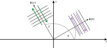
. The anisotropic flow kinematics for both
 $\unicode[STIX]{x1D713}$
and
 $\unicode[STIX]{x1D719}$
are illustrated in figure 2. As noted before, the stream function power spectrum is amplified in the direction of
 $\boldsymbol{s}(\unicode[STIX]{x1D703})$
, which by the transverse, skew-gradient nature of (2.4) implies that the horizontal velocity field is amplified in the direction perpendicular to
 $\boldsymbol{s}$
. For example, if
 $\unicode[STIX]{x1D703}$
is in the first quadrant then the amplified velocity direction will be in the second quadrant, and therefore
 $\mathbb{E}[uv]<0$
. Conversely, if the power spectra of
 $\unicode[STIX]{x1D719}$
are increased in the direction of
 $\boldsymbol{s}(\unicode[STIX]{x1D6FE})=(\cos \unicode[STIX]{x1D6FE},\sin \unicode[STIX]{x1D6FE})$
then
 $\boldsymbol{u}=\unicode[STIX]{x1D735}\unicode[STIX]{x1D719}$
is amplified in the same direction; in the depicted situation
 $\unicode[STIX]{x1D6FE}=\unicode[STIX]{x1D703}+\unicode[STIX]{x03C0}/2$
and the amplified velocity fields have the same direction.
Sketch of anisotropic flow kinematics. On the right is a Fourier component of the stream function with wavenumber vector
 $\boldsymbol{k}(\unicode[STIX]{x1D703})$
and angle
 $\unicode[STIX]{x1D703}$
in the first quadrant. The transversal flow indicated by the purple arrows is perpendicular to
 $\boldsymbol{k}(\unicode[STIX]{x1D703})$
. On the left is a Fourier component of the potential with wavenumber vector
 $\boldsymbol{k}(\unicode[STIX]{x1D6FE})$
and
 $\unicode[STIX]{x1D6FE}=\unicode[STIX]{x1D703}+\unicode[STIX]{x03C0}/2$
. The corresponding longitudinal flow indicated by the green arrows is parallel to
 $\boldsymbol{k}(\unicode[STIX]{x1D6FE})$
. Note that the flow fields are congruent and that
 $uv<0$
and
 $v^{2}>u^{2}$
.

In the sequel we will analyse the general case that features both
 $\unicode[STIX]{x1D713}$
and
 $\unicode[STIX]{x1D719}$
and formulate an anisotropic decomposition method for it. The principal advantage of our model is its simplicity and apparent self-consistent structure. Of course, the restriction to a single angle parameter
 $\unicode[STIX]{x1D703}$
or
 $\unicode[STIX]{x1D6FE}$
for all
 $k_{h}$
does not allow for the possibility that different anisotropy directions might be relevant at different length scales. This is certainly a restriction of practical importance. For example, oceanic jets tend to be highly anisotropic at large scales, but smaller submesoscale eddies tend to be fairly isotropic. Similarly, oceanic internal tides are expected to be anisotropic, but the background spectrum of internal waves described by the Garrett–Munk spectrum (e.g. Munk Reference Munk, Warren and Wunsch1981) is not. Presumably, in such a situation one could consider a superposition of models of the type (2.10) with different angles attached to different wavenumber regimes, but this is work for further research. However, we note that our tests with synthetic spectra in § 5.2 below include challenging cases that do not conform to the model assumptions, yet the method performs remarkably well.
3 Anisotropic Helmholtz decomposition
As was shown in BCF14, under the assumptions of isotropy and uncorrelated
 $\unicode[STIX]{x1D713}$
and
 $\unicode[STIX]{x1D719}$
, the one-dimensional power spectra can be uniquely decomposed into rotational and divergent parts by a suitable Helmholtz decomposition. The task here is to extend this result to our anisotropic models.
3.1 The Helmholtz decomposition
We consider the general case
 $$\begin{eqnarray}u=-\unicode[STIX]{x1D713}_{y}+\unicode[STIX]{x1D719}_{x}\quad \text{and}\quad v=\unicode[STIX]{x1D713}_{x}+\unicode[STIX]{x1D719}_{y}.\end{eqnarray}$$
With doubly periodic boundary conditions
 $\unicode[STIX]{x1D713}$
and
 $\unicode[STIX]{x1D719}$
are uniquely related to
 $u$
and
 $v$
(apart from meaningless constants), thus the Helmholtz decomposition can be found uniquely when the full velocity field
 $(u,v)$
as a function of
 $(x,y)$
is accessible. Of course, this result is not enough to allow such a decomposition when only ship-track data along the line
 $y=0$
are available. Additional assumptions are needed to make progress.
First off, we require that
 $\unicode[STIX]{x1D713}(x,y)$
and
 $\unicode[STIX]{x1D719}(x,y)$
are statistically uncorrelated such that
 $$\begin{eqnarray}\mathbb{E}[\unicode[STIX]{x1D713}(x_{0},y_{0})\unicode[STIX]{x1D719}(x_{0}+x,y_{0}+y)]=0\end{eqnarray}$$
for all
 $(x,y)$
. This is not a trivial requirement and its validity depends on the physical situation at hand, as discussed in BCF14. If (3.2) holds then the two-dimensional velocity spectra can be decomposed into a superposition of rotational and divergent parts via
 $$\begin{eqnarray}\left.\begin{array}{@{}c@{}}\displaystyle {\hat{C}}^{u}(k,l)={\hat{C}}_{\unicode[STIX]{x1D713}}^{u}(k,l)+{\hat{C}}_{\unicode[STIX]{x1D719}}^{u}(k,l)=+l^{2}{\hat{C}}^{\unicode[STIX]{x1D713}}(k,l)+k^{2}{\hat{C}}^{\unicode[STIX]{x1D719}}(k,l),\\ \displaystyle {\hat{C}}^{v}(k,l)={\hat{C}}_{\unicode[STIX]{x1D713}}^{v}(k,l)+{\hat{C}}_{\unicode[STIX]{x1D719}}^{v}(k,l)=+k^{2}{\hat{C}}^{\unicode[STIX]{x1D713}}(k,l)+l^{2}{\hat{C}}^{\unicode[STIX]{x1D719}}(k,l),\\ \displaystyle {\hat{C}}^{uv}(k,l)={\hat{C}}_{\unicode[STIX]{x1D713}}^{uv}(k,l)+{\hat{C}}_{\unicode[STIX]{x1D719}}^{uv}(k,l)=-kl{\hat{C}}^{\unicode[STIX]{x1D713}}(k,l)+kl{\hat{C}}^{\unicode[STIX]{x1D719}}(k,l).\end{array}\right\}\end{eqnarray}$$
Note that
 ${\hat{C}}^{uv}$
is manifestly real in this expression, or equivalently that
 $C^{uv}$
is an even function of
 $(x,y)$
. Hence the occurrence of an imaginary part of
 ${\hat{C}}^{uv}$
strictly implies a correlation between
 $\unicode[STIX]{x1D713}$
and
 $\unicode[STIX]{x1D719}$
, because (3.2) is the only assumption we have made so far. This yields a useful observational test of (3.2):
 $$\begin{eqnarray}\mathbb{E}[\unicode[STIX]{x1D713}(x_{0},y_{0})\unicode[STIX]{x1D719}(x_{0}+x,y_{0}+y)]=0\quad \Rightarrow \quad C^{uv}(x)=C^{uv}(-x)\quad \text{or}\quad {\hat{C}}^{uv}(k)\in R.\end{eqnarray}$$
This is unlikely to be a new result but we have not seen it pointed out elsewhere. Now, integrating (3.3) over the wavenumber
 $l$
(cf. (2.3)) yields
 $$\begin{eqnarray}\left.\begin{array}{@{}c@{}}\displaystyle {\hat{C}}^{u}(k)={\hat{C}}_{\unicode[STIX]{x1D713}}^{u}(k)+{\hat{C}}_{\unicode[STIX]{x1D719}}^{u}(k),\\ \displaystyle {\hat{C}}^{v}(k)={\hat{C}}_{\unicode[STIX]{x1D713}}^{v}(k)+{\hat{C}}_{\unicode[STIX]{x1D719}}^{v}(k),\\ \displaystyle {\hat{C}}^{uv}(k)={\hat{C}}_{\unicode[STIX]{x1D713}}^{uv}(k)+{\hat{C}}_{\unicode[STIX]{x1D719}}^{uv}(k).\end{array}\right\}\end{eqnarray}$$
The spectra on the left-hand side of (3.5) are observed and the spectra on the right-hand side are the sought-after Helmholtz decomposition. In BCF14, horizontal isotropy was assumed and hence only the first two lines in (3.5) had to be considered because under isotropy
 ${\hat{C}}^{uv}(k)$
is identically zero (this follows trivially from the even
 $l$
-integration of the odd integrand in the third row of (3.3)). Here we relax the isotropic assumption and develop a similar decomposition model that uses one extra quantity derived from the observations: the cross-correlation
 ${\hat{C}}^{uv}(k)$
.
3.2 Constraints on anisotropic one-dimensional spectra
We examine first the rotational component based on
 $\unicode[STIX]{x1D713}$
by assuming the spectrum
 $C^{\unicode[STIX]{x1D713}}(x,y)$
has the form (2.10) with some
 $\hat{F}(k_{h})$
,
 ${\hat{H}}(k_{h})$
and
 $\unicode[STIX]{x1D703}$
. Performing the
 $l$
-integration, noting that odd terms in
 $l$
vanish, and using
 $\cos 2\unicode[STIX]{x1D703}=\cos ^{2}\unicode[STIX]{x1D703}-\sin ^{2}\unicode[STIX]{x1D703}$
leads to
 $$\begin{eqnarray}\displaystyle {\hat{C}}_{\unicode[STIX]{x1D713}}^{u}(k) & = & \displaystyle \frac{1}{2\unicode[STIX]{x03C0}}\int _{-\infty }^{\infty }l^{2}[\hat{F}(k_{h})+(k^{2}\cos 2\unicode[STIX]{x1D703}+k_{h}^{2}\sin ^{2}\unicode[STIX]{x1D703}){\hat{H}}(k_{h})]\,\text{d}l,\end{eqnarray}$$
 $$\begin{eqnarray}\displaystyle {\hat{C}}_{\unicode[STIX]{x1D713}}^{v}(k) & = & \displaystyle \frac{1}{2\unicode[STIX]{x03C0}}\int _{-\infty }^{\infty }k^{2}[\hat{F}(k_{h})+(k^{2}\cos 2\unicode[STIX]{x1D703}+k_{h}^{2}\sin ^{2}\unicode[STIX]{x1D703}){\hat{H}}(k_{h})]\,\text{d}l,\end{eqnarray}$$
 $$\begin{eqnarray}\displaystyle {\hat{C}}_{\unicode[STIX]{x1D713}}^{uv}(k) & = & \displaystyle -\frac{1}{2\unicode[STIX]{x03C0}}\int _{-\infty }^{\infty }kl[(2kl\cos \unicode[STIX]{x1D703}\sin \unicode[STIX]{x1D703}){\hat{H}}(k_{h})]\,\text{d}l.\end{eqnarray}$$
These even integrals are equal to twice their values if
 $l\geqslant 0$
only. Hence, changing integration variable from
 $l\geqslant 0$
to
 $k_{h}\geqslant |k|$
and using
 $l\,\text{d}l=k_{h}\,\text{d}k_{h}$
at constant
 $k$
, we obtain
 $$\begin{eqnarray}\displaystyle {\hat{C}}_{\unicode[STIX]{x1D713}}^{u}(k) & = & \displaystyle \frac{1}{\unicode[STIX]{x03C0}}\int _{|k|}^{\infty }k_{h}\sqrt{k_{h}^{2}-k^{2}}[\hat{F}(k_{h})+(k^{2}\cos 2\unicode[STIX]{x1D703}+k_{h}^{2}\sin ^{2}\unicode[STIX]{x1D703}){\hat{H}}(k_{h})]\,\text{d}k_{h},\end{eqnarray}$$
 $$\begin{eqnarray}\displaystyle {\hat{C}}_{\unicode[STIX]{x1D713}}^{v}(k) & = & \displaystyle \frac{1}{\unicode[STIX]{x03C0}}\int _{|k|}^{\infty }\frac{k_{h}k^{2}}{\sqrt{k_{h}^{2}-k^{2}}}[\hat{F}(k_{h})+(k^{2}\cos 2\unicode[STIX]{x1D703}+k_{h}^{2}\sin ^{2}\unicode[STIX]{x1D703}){\hat{H}}(k_{h})]\,\text{d}k_{h},\end{eqnarray}$$
 $$\begin{eqnarray}\displaystyle {\hat{C}}_{\unicode[STIX]{x1D713}}^{uv}(k) & = & \displaystyle -\frac{\sin 2\unicode[STIX]{x1D703}}{\unicode[STIX]{x03C0}}\int _{|k|}^{\infty }k_{h}k^{2}\sqrt{k_{h}^{2}-k^{2}}{\hat{H}}(k_{h})\,\text{d}k_{h}.\end{eqnarray}$$
The last step uses
 $\sin 2\unicode[STIX]{x1D703}=2\cos \unicode[STIX]{x1D703}\sin \unicode[STIX]{x1D703}$
and confirms the heuristic link between
 $\unicode[STIX]{x1D703}$
and the sign of
 $\mathbb{E}[uv]$
noted at the end of § 2.2. Moreover, this makes clear that this link exists at every wavenumber.
By inspection and using Leibniz’s rule for differentiating integrals we obtain
 $$\begin{eqnarray}-k\frac{\text{d}}{\text{d}k}{\hat{C}}_{\unicode[STIX]{x1D713}}^{u}(k)={\hat{C}}_{\unicode[STIX]{x1D713}}^{v}(k)+2\cot 2\unicode[STIX]{x1D703}~{\hat{C}}_{\unicode[STIX]{x1D713}}^{uv}(k).\end{eqnarray}$$
Compared to the constraint derived for the isotropic model there is now a new term
 $2\cot 2\unicode[STIX]{x1D703}~{\hat{C}}_{\unicode[STIX]{x1D719}}^{uv}(k)$
. This term is straightforward to use numerically except when
 $\sin 2\unicode[STIX]{x1D703}$
vanishes, which occurs if
 $\unicode[STIX]{x1D703}=0$
or
 $\unicode[STIX]{x1D703}=\unicode[STIX]{x03C0}/2$
. In these cases the new term has a non-trivial limiting behaviour, because
 ${\hat{C}}_{\unicode[STIX]{x1D713}}^{uv}$
then vanishes as well, but this cannot easily be captured numerically. This is the Achilles heel case mentioned in (1.4).
Mutatis mutandis, for the divergent component depending on
 $\unicode[STIX]{x1D719}$
the counterparts of the above results can be derived in a similar fashion, so we skip the derivations and just list the results. We obtain
 $$\begin{eqnarray}\displaystyle {\hat{C}}_{\unicode[STIX]{x1D719}}^{u}(k) & = & \displaystyle \frac{1}{\unicode[STIX]{x03C0}}\int _{|k|}^{\infty }\frac{k_{h}k^{2}}{\sqrt{k_{h}^{2}-k^{2}}}[{\hat{G}}(k_{h})+(k^{2}\cos 2\unicode[STIX]{x1D6FE}+k_{h}^{2}\sin ^{2}\unicode[STIX]{x1D6FE})\hat{I} (k_{h})]\,\text{d}k_{h},\end{eqnarray}$$
 $$\begin{eqnarray}\displaystyle {\hat{C}}_{\unicode[STIX]{x1D719}}^{v}(k) & = & \displaystyle \frac{1}{\unicode[STIX]{x03C0}}\int _{|k|}^{\infty }k_{h}\sqrt{k_{h}^{2}-k^{2}}[{\hat{G}}(k_{h})+(k^{2}\cos 2\unicode[STIX]{x1D6FE}+k_{h}^{2}\sin ^{2}\unicode[STIX]{x1D6FE})\hat{I} (k_{h})]\,\text{d}k_{h},\end{eqnarray}$$
 $$\begin{eqnarray}\displaystyle {\hat{C}}_{\unicode[STIX]{x1D719}}^{uv}(k) & = & \displaystyle +\frac{\sin 2\unicode[STIX]{x1D6FE}}{\unicode[STIX]{x03C0}}\int _{|k|}^{\infty }k_{h}k^{2}\sqrt{k_{h}^{2}-k^{2}}\hat{I} (k_{h})\,\text{d}k_{h},\end{eqnarray}$$
and this counterpart to (3.12):
 $$\begin{eqnarray}-k\frac{\text{d}}{\text{d}k}{\hat{C}}_{\unicode[STIX]{x1D719}}^{v}(k)={\hat{C}}_{\unicode[STIX]{x1D719}}^{u}(k)-2\cot 2\unicode[STIX]{x1D6FE}\,{\hat{C}}_{\unicode[STIX]{x1D719}}^{uv}(k).\end{eqnarray}$$
Note the different sign in the final term compared to (3.12). We note in passing that in BCF14 the functions
 ${\hat{C}}_{\unicode[STIX]{x1D713}}^{u}$
and
 ${\hat{C}}_{\unicode[STIX]{x1D719}}^{v}$
were denoted by
 $D^{\unicode[STIX]{x1D713}}$
and
 $D^{\unicode[STIX]{x1D719}}$
, respectively. The present notation is clearer and makes obvious the physical meaning of these functions.
3.3 Model choice and decomposition method
At this juncture the most natural step would be to allow anisotropy of the described form in both
 $\unicode[STIX]{x1D713}$
and
 $\unicode[STIX]{x1D719}$
and then determine the relevant spectral functions from the observed data. However, a simple counting argument shows that this not possible in general. This is because observing the three one-dimensional spectra
 $({\hat{C}}^{u},{\hat{C}}^{v},{\hat{C}}^{uv})$
is not enough to determine the four underlying spectral functions
 $(\hat{F},{\hat{G}},{\hat{H}},\hat{I} )$
that appear in (2.10) and (2.14). If a decomposition of both
 ${\hat{C}}^{u}$
and
 ${\hat{C}}^{v}$
is required then we need to proceed with a more modest modelling step that allows anisotropy in either
 $\unicode[STIX]{x1D713}$
or
 $\unicode[STIX]{x1D719}$
but not in both simultaneously. In other words, we attribute the anisotropy at the outset to either
 $\unicode[STIX]{x1D713}$
or
 $\unicode[STIX]{x1D719}$
. This is a significant restriction, no doubt, although physical circumstances can be envisaged where anisotropy is indeed dominant in only one of the two fields. For example, if a dominant balanced flow is anisotropic but the waves are not then
 $\unicode[STIX]{x1D719}$
could be modelled isotropically to good approximation.
However, it will turn out that the decomposition of the kinetic energy spectrum
 $K=({\hat{C}}^{u}+{\hat{C}}^{v})/2$
will be indifferent to the choice of anisotropy attribution. In other words, whereas the individual decomposition of
 ${\hat{C}}^{u}$
and
 ${\hat{C}}^{v}$
depends on that attribution choice, their sum is indifferent to it. Indeed, there is a whole family of jointly anisotropic flow models in both
 $\unicode[STIX]{x1D713}$
and
 $\unicode[STIX]{x1D719}$
that yield the identical decomposition of
 $K$
. This important fact, which has significant implications for the wave–vortex decomposition, will be discussed in § 3.4.
Leaving aside the determination of the scalar angle parameters
 $\unicode[STIX]{x1D703}$
and
 $\unicode[STIX]{x1D6FE}$
for the moment, we now identify two alternative models suitable for a full decomposition of both
 ${\hat{C}}^{u}$
and
 ${\hat{C}}^{v}$
:
Model 1. (Anisotropic stream function model) The power spectrum of
 $\unicode[STIX]{x1D713}$
has the anisotropic form (2.10), but for
 $\unicode[STIX]{x1D719}$
we set
 $\hat{I} (k_{h})\equiv 0$
in (2.14). This implies
 ${\hat{C}}_{\unicode[STIX]{x1D713}}^{uv}(k)={\hat{C}}^{uv}(k)$
and
 $\unicode[STIX]{x1D6FE}$
is irrelevant.
Model 2. (Anisotropic potential model) Here the power spectrum
 $\unicode[STIX]{x1D719}$
has the anisotropic form (2.14), but we set
 ${\hat{H}}(k_{h})\equiv 0$
in (2.10). This implies
 ${\hat{C}}_{\unicode[STIX]{x1D719}}^{uv}(k)={\hat{C}}^{uv}(k)$
and
 $\unicode[STIX]{x1D703}$
is irrelevant.
Combining (3.5) with either (3.12) or (3.16) the corresponding decomposition equations are either
 $$\begin{eqnarray}\text{Model 1:}\quad \left\{\begin{array}{@{}c@{}}\displaystyle -k\frac{\text{d}}{\text{d}k}{\hat{C}}_{\unicode[STIX]{x1D713}}^{u}(k)+{\hat{C}}_{\unicode[STIX]{x1D719}}^{v}(k)={\hat{C}}^{v}(k)+2\cot 2\unicode[STIX]{x1D703}\,{\hat{C}}^{uv}(k),\\ \displaystyle {\hat{C}}_{\unicode[STIX]{x1D713}}^{u}(k)-k\frac{\text{d}}{\text{d}k}{\hat{C}}_{\unicode[STIX]{x1D719}}^{v}(k)={\hat{C}}^{u}(k),\end{array}\right.\end{eqnarray}$$
or
 $$\begin{eqnarray}\text{Model 2:}\quad \left\{\begin{array}{@{}c@{}}\displaystyle -k\frac{\text{d}}{\text{d}k}{\hat{C}}_{\unicode[STIX]{x1D713}}^{u}(k)+{\hat{C}}_{\unicode[STIX]{x1D719}}^{v}(k)={\hat{C}}^{v}(k),\\ \displaystyle {\hat{C}}_{\unicode[STIX]{x1D713}}^{u}(k)-k\frac{\text{d}}{\text{d}k}{\hat{C}}_{\unicode[STIX]{x1D719}}^{v}(k)={\hat{C}}^{u}(k)-2\cot 2\unicode[STIX]{x1D6FE}\,{\hat{C}}^{uv}(k).\end{array}\right.\end{eqnarray}$$
The spectra on the right-hand side are observed so this is a set of ordinary differential equations (ODEs) for
 ${\hat{C}}_{\unicode[STIX]{x1D713}}^{u}(k)$
and
 ${\hat{C}}_{\unicode[STIX]{x1D719}}^{v}(k)$
, which can be solved backwards from
 $k=+\infty$
to
 $k=0$
after using the decay boundary conditions
 $$\begin{eqnarray}{\hat{C}}_{\unicode[STIX]{x1D719}}^{v}(+\infty )={\hat{C}}_{\unicode[STIX]{x1D713}}^{u}(+\infty )=0.\end{eqnarray}$$
As noted in BCF14, these ODE systems diagonalize in the variables
 ${\hat{C}}_{\unicode[STIX]{x1D713}}^{u}\pm {\hat{C}}_{\unicode[STIX]{x1D719}}^{v}$
, which allows their explicit solution. For the first model the solution for
 $k\geqslant 0$
is
 $$\begin{eqnarray}\displaystyle {\hat{C}}_{\unicode[STIX]{x1D713}}^{u}(k)=\int _{k}^{\infty }\frac{1}{2\bar{k}}\left[{\hat{C}}^{u}(\bar{k})\frac{k^{2}-\bar{k}^{2}}{\bar{k}k}+[{\hat{C}}^{v}(\bar{k})+2\cot 2\unicode[STIX]{x1D703}{\hat{C}}^{uv}(\bar{k})]\frac{k^{2}+\bar{k}^{2}}{\bar{k}k}\right]\,\text{d}\bar{k}, & & \displaystyle\end{eqnarray}$$
 $$\begin{eqnarray}\displaystyle {\hat{C}}_{\unicode[STIX]{x1D719}}^{v}(k)=\int _{k}^{\infty }\frac{1}{2\bar{k}}\left[{\hat{C}}^{u}(\bar{k})\frac{k^{2}+\bar{k}^{2}}{\bar{k}k}+[{\hat{C}}^{v}(\bar{k})+2\cot 2\unicode[STIX]{x1D703}{\hat{C}}^{uv}(\bar{k})]\frac{k^{2}-\bar{k}^{2}}{\bar{k}k}\right]\,\text{d}\bar{k}. & & \displaystyle\end{eqnarray}$$
These extend the equations (2.30)–(2.31) of BCF14, where
 $(D^{\unicode[STIX]{x1D713}},D^{\unicode[STIX]{x1D719}},s)$
correspond to
 $({\hat{C}}_{\unicode[STIX]{x1D713}}^{u},{\hat{C}}_{\unicode[STIX]{x1D719}}^{v},\ln k)$
here. For the second model we find
 $$\begin{eqnarray}\displaystyle {\hat{C}}_{\unicode[STIX]{x1D713}}^{u}(k)=\int _{k}^{\infty }\frac{1}{2\bar{k}}\left[[{\hat{C}}^{u}(\bar{k})-2\cot 2\unicode[STIX]{x1D6FE}{\hat{C}}^{uv}(\bar{k})]\frac{k^{2}-\bar{k}^{2}}{\bar{k}k}+{\hat{C}}^{v}(\bar{k})\frac{k^{2}+\bar{k}^{2}}{\bar{k}k}\right]\,\text{d}\bar{k}, & & \displaystyle\end{eqnarray}$$
 $$\begin{eqnarray}\displaystyle {\hat{C}}_{\unicode[STIX]{x1D719}}^{v}(k)=\int _{k}^{\infty }\frac{1}{2\bar{k}}\left[[{\hat{C}}^{u}(\bar{k})-2\cot 2\unicode[STIX]{x1D6FE}{\hat{C}}^{uv}(\bar{k})]\frac{k^{2}+\bar{k}^{2}}{\bar{k}k}+{\hat{C}}^{v}(\bar{k})\frac{k^{2}-\bar{k}^{2}}{\bar{k}k}\right]\,\text{d}\bar{k}. & & \displaystyle\end{eqnarray}$$
With
 $({\hat{C}}_{\unicode[STIX]{x1D713}}^{u},{\hat{C}}_{\unicode[STIX]{x1D719}}^{v})$
in hand the other decomposition members then follow as
 $$\begin{eqnarray}{\hat{C}}_{\unicode[STIX]{x1D719}}^{u}(k)={\hat{C}}^{u}(k)-{\hat{C}}_{\unicode[STIX]{x1D713}}^{u}(k)\quad \text{and}\quad {\hat{C}}_{\unicode[STIX]{x1D713}}^{v}(k)={\hat{C}}^{v}(k)-{\hat{C}}_{\unicode[STIX]{x1D719}}^{v}(k).\end{eqnarray}$$
It remains to determine the relevant angle parameter, which is in fact straightforward from the bulk statistics of the data. For example, in order to find
 $\unicode[STIX]{x1D703}$
in the first model we integrate both equations in (3.17) over
 $k$
and then subtract them. This yields
 $$\begin{eqnarray}\cot 2\unicode[STIX]{x1D703}=\frac{\mathbb{E}u^{2}-\mathbb{E}v^{2}}{2\mathbb{E}uv}\quad \text{and}\quad \text{sgn}(\sin 2\unicode[STIX]{x1D703})=-\text{sgn}(\mathbb{E}uv).\end{eqnarray}$$
The latter is the sign relation established earlier. This concludes the unique determination of
 $\unicode[STIX]{x1D703}\in [0,\unicode[STIX]{x03C0})$
, which the first part of (3.25) only determines up to a difference of
 $\unicode[STIX]{x03C0}/2$
. Notice that in order to compute
 $\unicode[STIX]{x1D703}$
we do not need the spectral functions, since we can calculate the statistics
 $\mathbb{E}u^{2}-\mathbb{E}v^{2}$
and
 $\mathbb{E}uv$
directly from the velocity observations. Similarly, for
 $\unicode[STIX]{x1D6FE}$
in the second model we obtain
 $$\begin{eqnarray}\cot 2\unicode[STIX]{x1D6FE}=\frac{\mathbb{E}u^{2}-\mathbb{E}v^{2}}{2\mathbb{E}uv}\quad \text{and}\quad \text{sgn}(\sin 2\unicode[STIX]{x1D6FE})=+\text{sgn}(\mathbb{E}uv),\end{eqnarray}$$
which differs from (3.25) only in the sign condition. Therefore, for the same data
 $\unicode[STIX]{x1D703}$
and
 $\unicode[STIX]{x1D6FE}$
differ by
 $\unicode[STIX]{x03C0}/2$
, i.e. the corresponding directions are perpendicular as illustrated in figure 2. This does not depend on the nature of the data but is a feature of our method. Overall
 $\unicode[STIX]{x1D6FE}$
and
 $\unicode[STIX]{x1D703}$
point into the first and second principal directions of the random velocity field in
 $uv$
-space, respectively. In particular, we can use the substitution
 $$\begin{eqnarray}2\cot 2\unicode[STIX]{x1D703}=2\cot 2\unicode[STIX]{x1D6FE}=\frac{\mathbb{E}u^{2}-\mathbb{E}v^{2}}{\mathbb{E}uv}\end{eqnarray}$$
in the solution formulas derived above. This works except in the Achilles heel case
 $\mathbb{E}uv=0$
but
 $\mathbb{E}u^{2}\neq \mathbb{E}v^{2}$
.
3.4 Kinetic energy spectrum decomposition
The Helmholtz decomposition of the horizontal kinetic energy spectrum
 $$\begin{eqnarray}K={\textstyle \frac{1}{2}}({\hat{C}}^{u}+{\hat{C}}^{v})=K^{\unicode[STIX]{x1D713}}+K^{\unicode[STIX]{x1D719}}\end{eqnarray}$$
naturally involves
 $$\begin{eqnarray}2K^{\unicode[STIX]{x1D713}}(k)={\hat{C}}_{\unicode[STIX]{x1D713}}^{u}(k)+{\hat{C}}_{\unicode[STIX]{x1D713}}^{v}(k)\quad \text{and}\quad 2K^{\unicode[STIX]{x1D719}}(k)={\hat{C}}_{\unicode[STIX]{x1D719}}^{u}(k)+{\hat{C}}_{\unicode[STIX]{x1D719}}^{v}(k).\end{eqnarray}$$
Substituting from the exact solution (3.20)–(3.26) and using
 $k\geqslant 0$
leads to
 $$\begin{eqnarray}\displaystyle 2K^{\unicode[STIX]{x1D713}}(k) & = & \displaystyle {\hat{C}}^{v}(k)+\frac{1}{k}\int _{k}^{\infty }\left({\hat{C}}^{v}(\bar{k})-{\hat{C}}^{u}(\bar{k})+\frac{\mathbb{E}u^{2}-\mathbb{E}v^{2}}{\mathbb{E}uv}{\hat{C}}^{uv}(\bar{k})\right)\,\text{d}\bar{k},\end{eqnarray}$$
 $$\begin{eqnarray}\displaystyle 2K^{\unicode[STIX]{x1D719}}(k) & = & \displaystyle {\hat{C}}^{u}(k)-\frac{1}{k}\int _{k}^{\infty }\left({\hat{C}}^{v}(\bar{k})-{\hat{C}}^{u}(\bar{k})+\frac{\mathbb{E}u^{2}-\mathbb{E}v^{2}}{\mathbb{E}uv}{\hat{C}}^{uv}(\bar{k})\right)\,\text{d}\bar{k}.\end{eqnarray}$$
Without the new anisotropic term in
 ${\hat{C}}^{uv}$
these expressions were first displayed in Lindborg (Reference Lindborg2015) as a trivial but useful consequence of the Helmholtz decomposition method in BCF14. Surprisingly, these formulas are valid for both models, i.e. any set of input spectra
 $({\hat{C}}^{u},{\hat{C}}^{v},{\hat{C}}^{uv})$
leads to predictions for
 $(K^{\unicode[STIX]{x1D713}},K^{\unicode[STIX]{x1D719}})$
that are identical for both anisotropic models. Crucially, as discussed in the next section, the only ingredient from the Helmholtz decomposition that enters into the wave–vortex decomposition is
 $K^{\unicode[STIX]{x1D719}}$
, which by (3.31) is the same for both anisotropic models. So even a ‘wrong’ anisotropic model choice for the Helmholtz decomposition would not affect the subsequent wave–vortex decomposition.
This surprising result warrants some more analysis: why does the model choice not matter for the energy decomposition? First, rewriting
 $K^{\unicode[STIX]{x1D713}}$
as
 $$\begin{eqnarray}2K^{\unicode[STIX]{x1D713}}(k)={\hat{C}}_{\unicode[STIX]{x1D713}}^{u}(k)+{\hat{C}}_{\unicode[STIX]{x1D713}}^{v}(k)={\hat{C}}_{\unicode[STIX]{x1D713}}^{u}(k)-{\hat{C}}_{\unicode[STIX]{x1D719}}^{v}(k)+{\hat{C}}^{v}(k)\end{eqnarray}$$
shows that
 $K^{\unicode[STIX]{x1D713}}$
depends only on the difference
 ${\hat{C}}_{\unicode[STIX]{x1D713}}^{u}-{\hat{C}}_{\unicode[STIX]{x1D719}}^{v}$
of the spectra appearing in the ODE systems (3.17) or (3.18). Second, this difference satisfies the respective ODEs
 $$\begin{eqnarray}-\!\left(k\frac{\text{d}}{\text{d}k}+1\right)({\hat{C}}_{\unicode[STIX]{x1D713}}^{u}(k)-{\hat{C}}_{\unicode[STIX]{x1D719}}^{v}(k))=\left\{\begin{array}{@{}ll@{}}{\hat{C}}^{v}(k)-{\hat{C}}^{u}(k)+2\cot 2\unicode[STIX]{x1D703}\,{\hat{C}}^{uv}(k)\quad & \text{M1}\\ {\hat{C}}^{v}(k)-{\hat{C}}^{u}(k)+2\cot 2\unicode[STIX]{x1D6FE}\,{\hat{C}}^{uv}(k)\quad & \text{M2}\end{array}\right.\end{eqnarray}$$
in the two models. This makes obvious that
 $K^{\unicode[STIX]{x1D713}}$
is indifferent to the model choice if
 $\cot 2\unicode[STIX]{x1D6FE}=\cot 2\unicode[STIX]{x1D703}$
, which is of course the case here.
This derivation highlights a relevant symmetry of the ODE systems (3.17) and (3.18): the kinetic energy decomposition is indifferent to any function that is added to both equations on the right-hand side, because this leaves the difference equation unchanged. This allows for a virtual third model to be conceived in which both
 $\unicode[STIX]{x1D713}$
and
 $\unicode[STIX]{x1D719}$
are allowed to be anisotropic, but it is required that the anisotropy direction is the same in both fields such that (3.27) holds:
 $$\begin{eqnarray}\text{Model 3:}\quad \left\{\begin{array}{@{}c@{}}\displaystyle -k\frac{\text{d}}{\text{d}k}{\hat{C}}_{\unicode[STIX]{x1D713}}^{u}(k)+{\hat{C}}_{\unicode[STIX]{x1D719}}^{v}(k)={\hat{C}}^{v}(k)+\displaystyle \frac{\mathbb{E}u^{2}-\mathbb{E}v^{2}}{\mathbb{E}uv}\,{\hat{C}}_{\unicode[STIX]{x1D713}}^{uv}(k),\\ \displaystyle {\hat{C}}_{\unicode[STIX]{x1D713}}^{u}(k)-k\frac{\text{d}}{\text{d}k}{\hat{C}}_{\unicode[STIX]{x1D719}}^{v}(k)={\hat{C}}^{u}(k)-\displaystyle \frac{\mathbb{E}u^{2}-\mathbb{E}v^{2}}{\mathbb{E}uv}\,{\hat{C}}_{\unicode[STIX]{x1D719}}^{uv}(k).\end{array}\right.\end{eqnarray}$$
For example, this would be a physically appealing model in a situation with strong anisotropic inertia–gravity waves, which affects both
 $\unicode[STIX]{x1D713}$
and
 $\unicode[STIX]{x1D719}$
. Of course, such a model would have non-zero
 ${\hat{C}}_{\unicode[STIX]{x1D713}}^{uv}$
as well as
 ${\hat{C}}_{\unicode[STIX]{x1D719}}^{uv}$
and by the standard counting argument it could not be solved for all the decomposed fields. However, it could be solved for the kinetic energy decomposition because the relevant difference equation
 $$\begin{eqnarray}-\!\left(k\frac{\text{d}}{\text{d}k}+1\right)({\hat{C}}_{\unicode[STIX]{x1D713}}^{u}(k)-{\hat{C}}_{\unicode[STIX]{x1D719}}^{v}(k))={\hat{C}}^{v}(k)-{\hat{C}}^{u}(k)+\displaystyle \frac{\mathbb{E}u^{2}-\mathbb{E}v^{2}}{\mathbb{E}uv}\,{\hat{C}}^{uv}(k)\end{eqnarray}$$
would only contain the observed
 ${\hat{C}}^{uv}={\hat{C}}_{\unicode[STIX]{x1D713}}^{uv}+{\hat{C}}_{\unicode[STIX]{x1D719}}^{uv}$
. This would again yield the same answer for
 $K^{\unicode[STIX]{x1D713}}$
as the two other models, i.e. (3.35) holds for all three models. The fact that the all-important Helmholtz decomposition of the kinetic energy is indifferent to the model choice lends some robustness to our results.
4 Wave–vortex decomposition
In BCF14 a two-step procedure for horizontally isotropic spectra was developed in which the first step was a Helmholtz decomposition of the horizontal velocity spectra and the second step utilized results from linear inertia–gravity wave theory to estimate the wave energy spectrum solely from the observed velocity fields. The second step relied on the additional assumptions of stationarity in time and vertical homogeneity, which allowed modelling the wave field as an uncorrelated superposition of plane waves. The present paper is focused on extending the Helmholtz decomposition of the first step to anisotropic spectra, but here we point out that the second step of estimating the wave energy spectrum goes through under the same assumptions as in the isotropic case studied in BCF14.
4.1 Inertia–gravity wave energy spectrum
The key of the argument in BCF14 is to exploit an energy equipartition property valid for an uncorrelated superposition of three-dimensional plane inertia–gravity waves if the Coriolis parameter
 $f$
and the buoyancy frequency
 $N$
are constant. Assume first that the flow field is entirely due to linear inertia–gravity waves. The wave energy spectrum is generally defined as
 $$\begin{eqnarray}E_{W}={\textstyle \frac{1}{2}}({\hat{C}}_{W}^{b}+{\hat{C}}_{W}^{u}+{\hat{C}}_{W}^{v}+{\hat{C}}_{W}^{w}),\end{eqnarray}$$
where
 ${\hat{C}}_{W}^{b}$
is the power spectrum of
 $b/N$
if
 $b$
is the buoyancy disturbance such that
 $b_{t}=-N^{2}w$
and the remaining terms are the spectra of three-dimensional velocity components
 $(u,v,w)$
, respectively. The subscript
 $W$
indicates that these spectra pertain to the wave field only. For one-dimensional spectra we can use (3.29) to put (4.1) into the form
 $$\begin{eqnarray}E_{W}(k)={\textstyle \frac{1}{2}}({\hat{C}}_{W}^{b}(k)+2K_{W}^{\unicode[STIX]{x1D713}}(k)+2K_{W}^{\unicode[STIX]{x1D719}}(k)+{\hat{C}}_{W}^{w}(k)).\end{eqnarray}$$
Now, in § A.2 of BCF14 it was shown that for uncorrelated plane waves the following energy equipartition holds:
 $$\begin{eqnarray}{\hat{C}}_{W}^{b}(k)+2K_{W}^{\unicode[STIX]{x1D713}}(k)=2K_{W}^{\unicode[STIX]{x1D719}}(k)+{\hat{C}}_{W}^{w}(k).\end{eqnarray}$$
The derivation of (4.3) uses the full three-dimensional structure and dispersion relation of inertia–gravity waves and does not assume horizontal isotropy. Hence (4.3) is in fact valid for anisotropic spectra as well, including spectra of the form assumed in this paper. Moreover, the argument in favour of uncorrelated
 $\unicode[STIX]{x1D713}$
and
 $\unicode[STIX]{x1D719}$
for internal waves that is given in A.1 of BCF14 also carries over, because the key part of that argument was that there be no preferred orientation of the horizontal wave propagation. This covers our anisotropic case, because although the vector
 $\boldsymbol{s}$
singles out a preferential direction, just as many waves are travelling in the direction
 $+\boldsymbol{s}$
as in
 $-\boldsymbol{s}$
, so there is no preferred orientation. Combining (4.3) and (4.2) yields the key result
 $$\begin{eqnarray}E_{W}(k)=2K_{W}^{\unicode[STIX]{x1D719}}(k)+{\hat{C}}_{W}^{w}(k).\end{eqnarray}$$
For hydrostatic waves the second term is negligible, which is often appropriate for low-resolution measurements.
4.2 Waves and geostrophic flow
The previous section assumed that the flow consisted entirely of linear inertia–gravity waves, but it is straightforward to extend this scenario to an uncorrelated superposition of such waves together with a linear vortical flow in geostrophic and hydrostatic balance. This is the kind of vortical flow associated with quasi-geostrophic dynamics. The key observation here is that such a linear flow is horizontally non-divergent (i.e. there is no potential
 $\unicode[STIX]{x1D719}$
associated with the linear balanced flow at leading order) and also has no vertical velocity. This means we can assume that
 $$\begin{eqnarray}{\hat{C}}^{\unicode[STIX]{x1D719}}={\hat{C}}_{W}^{\unicode[STIX]{x1D719}}\quad \text{and}\quad {\hat{C}}^{w}={\hat{C}}_{W}^{w}.\end{eqnarray}$$
Hence
 $K^{\unicode[STIX]{x1D719}}(k)=K_{W}^{\unicode[STIX]{x1D719}}(k)$
holds, which allows rewriting (4.4) in the final form
 $$\begin{eqnarray}E_{W}(k)=2K^{\unicode[STIX]{x1D719}}(k)+{\hat{C}}^{w}(k).\end{eqnarray}$$
The first term is computed from the Helmholtz decomposition as in (3.31) and the second term is directly observed (or ignored for hydrostatic waves). As discussed in BCF14, this provides an estimate of wave energy based solely on velocity measurements. If the total energy is measured as well, as would be the case if the buoyancy spectrum
 ${\hat{C}}^{b}$
is observed, then (4.6) can be used to decompose the observed flow energy into wave and vortex components. Notably, horizontal anisotropy of the data enters this process only indirectly, namely by affecting the outcome of the Helmholtz decomposition that is required to compute
 $K^{\unicode[STIX]{x1D719}}(k)$
. As noted before,
 $K^{\unicode[STIX]{x1D719}}(k)$
is indifferent to the model choice, which hence does not affect the predicted wave energy either. But allowing for anisotropy in the first place does matter, as was made obvious by the anisotropic corrections in (3.31) and (4.7).
Finally, we note that because
 $\mathbb{E}uv$
and
 ${\hat{C}}^{uv}$
have the same sign by assumption, we can read off the sign of the anisotropic contribution to
 $K^{\unicode[STIX]{x1D713}}$
and
 $K^{\unicode[STIX]{x1D719}}$
from (3.30) and (3.31). Specifically, if
 $\mathbb{E}u^{2}>\mathbb{E}v^{2}$
then the anisotropic
 $K^{\unicode[STIX]{x1D713}}$
is larger than its isotropic counterpart at all wavenumbers
 $k$
, whilst the opposite is true for
 $K^{\unicode[STIX]{x1D719}}$
, i.e.
 $$\begin{eqnarray}K^{\unicode[STIX]{x1D713}}(k)-K_{iso}^{\unicode[STIX]{x1D713}}(k)\propto \mathbb{E}[u^{2}-v^{2}]\quad \text{and}\quad K^{\unicode[STIX]{x1D719}}(k)-K_{iso}^{\unicode[STIX]{x1D719}}(k)\propto \mathbb{E}[v^{2}-u^{2}].\end{eqnarray}$$
These relations are useful checks on the numerical results but we have not been able to establish a clear physical interpretation of them.
5 Application to data
Our point of departure are the observed one-dimensional spectra
 $({\hat{C}}^{u},{\hat{C}}^{v},{\hat{C}}^{uv})$
. Of course, the accurate estimation of these spectra from noisy sets of discrete observations along real flight or ship tracks may itself be a non-trivial task, but we will not consider this problem in this paper. For the ocean observation reported in § 5.3 below, we simply adopted the methodology introduced in Callies & Ferrari (Reference Callies and Ferrari2013) and Callies et al. (Reference Callies, Ferrari, Klymak and Gula2015), to which we refer the readers for details. The main task here is how to establish the admissibility of our spectral models and to select the optimal choice of model.
5.1 Model selection and stability
Our spectral models are characterized by the no-correlation condition (3.2) and the specific anisotropy defined in (2.10) or (2.14). As noted below (3.3), if
 $\unicode[STIX]{x1D713}$
and
 $\unicode[STIX]{x1D719}$
are uncorrelated then
 ${\hat{C}}^{uv}(k)$
is a real-valued function, or equivalently
 $C^{uv}(x)$
is an even function of
 $x$
. This itself is an interesting result, namely that the fingerprint of correlated
 $\unicode[STIX]{x1D713}$
and
 $\unicode[STIX]{x1D719}$
is an imaginary part of
 ${\hat{C}}^{uv}$
. The upshot is that for our models to be admissible in a practical situation it is necessary that the imaginary part of the observed
 ${\hat{C}}^{uv}$
be negligible.
Moreover, the spectral anisotropy assumed in (2.10) or (2.14) implies that the one-dimensional
 ${\hat{C}}^{uv}(k)$
in (3.11) or (3.15) is not just real but also sign-definite for all
 $k$
. This is hence another test that real data must pass to good approximation, i.e. there should be no sign changes in the cross-spectrum. Finally, the angle parameters
 $\unicode[STIX]{x1D703}$
or
 $\unicode[STIX]{x1D6FE}$
must be estimated from (3.25) or (3.26), which is straightforward except in the aforementioned Achilles heel case in which
 $\mathbb{E}u^{2}\neq \mathbb{E}v^{2}$
, but
 $\mathbb{E}uv$
is zero. In this case
 $\cot 2\unicode[STIX]{x1D703}$
or
 $\cot 2\unicode[STIX]{x1D6FE}$
would be infinite, which leads to indeterminate forms in the model equations (3.17) or (3.18). Hence in this case it is not possible to admit either of our anisotropic models, even though the data are clearly anisotropic by virtue of
 $\mathbb{E}u^{2}\neq \mathbb{E}v^{2}$
.
Overall, we followed this procedure for model selection.
-
(i) Calculate
 $\mathbb{E}u^{2}-\mathbb{E}v^{2}$
and
$\mathbb{E}uv$
. If both are zero select the isotropic model.
-
(ii) Otherwise, if
$\mathbb{E}uv\neq 0$
check that the imaginary part of
${\hat{C}}^{uv}(k)$
is negligible and that the real part of
${\hat{C}}^{uv}(k)$
is sign-definite. If both are true select one of the anisotropic models, compute the corresponding angle parameter, and proceed with the decomposition. If either fails, warn the user that neither model is admissible. -
(iii) Otherwise, if
$\mathbb{E}uv=0$
and
$\mathbb{E}u^{2}-\mathbb{E}v^{2}\neq 0$
, select the isotropic model for decomposition, but warn the user that the data are actually anisotropic. (This is the Achilles heel case.)


If the anisotropic models are admissible then one can try them and establish which one gives a better result. There might be physical reasons to favour the anisotropic stream function model (e.g. dominance of vortices) or the anisotropic potential model (e.g. dominance of inertia–gravity waves), but there are also mathematical considerations. For example, using the wrong model can lead to non-physical decomposition results such as negative or divergent velocity spectra in (3.20)–(3.24). Again, for the purpose of decomposing the kinetic energy spectrum in (3.30) and (3.31) the model choice does not matter.
Finally, in real datasets the observed spectra will be subject to noise and hence the stability of our method under noisy observations is an issue. An important practical consideration in this context is what happens if the underlying process is isotropic, say, but both of the empirical statistics
 $\mathbb{E}u^{2}-\mathbb{E}v^{2}$
and
 $\mathbb{E}uv$
are non-zero due to observational noise and sampling errors. Then a natural question is whether selecting an anisotropic model for data that are ‘almost isotropic’ will result in an anisotropic decomposition close to the isotropic one or not. This is a question of stability for the decomposition method: do small changes in the data lead to small changes in the decomposition or not? Notice that when
 $\mathbb{E}uv$
and
 $\mathbb{E}u^{2}-v^{2}$
are close to zero, the angle parameters
 $\unicode[STIX]{x1D703}$
or
 $\unicode[STIX]{x1D6FE}$
will be unstable. Thus one might doubt whether the resulting anisotropic decomposition will converge to the isotropic one. The following result, however, guarantees this convergence.
We give the argument for the first model but it works for either model. Suppose
 ${\hat{C}}^{uv}(k)$
is real and sign-definite. Define
 $D_{\unicode[STIX]{x1D713}}^{iso}(k)$
as the isotropic solution and
 $D_{\unicode[STIX]{x1D713}}^{ani}(k)$
as the anisotropic solution from (3.20). Here the isotropic solution simply omits the cross-spectrum terms. Then (3.20) yields
 $$\begin{eqnarray}D_{\unicode[STIX]{x1D713}}^{ani}(k)-D_{\unicode[STIX]{x1D713}}^{iso}(k)=\frac{\cot 2\unicode[STIX]{x1D703}}{k}\int _{k}^{\infty }{\hat{C}}^{uv}(\bar{k})\frac{k^{2}+\bar{k}^{2}}{\bar{k}^{2}}\,\text{d}\bar{k}.\end{eqnarray}$$
The cross-spectrum does not change sign by assumption and the rational factor is bounded by
 $2$
, therefore
 $$\begin{eqnarray}|D_{\unicode[STIX]{x1D713}}^{ani}(k)-D_{\unicode[STIX]{x1D713}}^{iso}(k)|<\left|\frac{2}{k}\cot 2\unicode[STIX]{x1D703}\int _{0}^{\infty }{\hat{C}}^{uv}(\bar{k})\,\text{d}\bar{k}\right|<\left|\frac{2\unicode[STIX]{x03C0}}{k}\cot 2\unicode[STIX]{x1D703}\mathbb{E}uv\right|<\left|\frac{\unicode[STIX]{x03C0}}{k}\mathbb{E}[u^{2}-v^{2}]\right|.\end{eqnarray}$$
The last step uses (3.25) and establishes the sought-after stability result. A similar result obviously holds for the kinetic energy spectra in (3.30) and (3.31). This implies that for any wavenumber
 $k>0$
the anisotropic decomposition converges to the isotropic decomposition if
 $\mathbb{E}u^{2}-\mathbb{E}v^{2}$
goes to zero. It also shows that anisotropic effects are stronger for small wavenumbers. Indeed, the convergence is non-uniform at
 $k=0$
, as could be expected from the solution integral (3.20), the existence of which at
 $k=0$
relies on the observed power spectra going to zero there. This will always be the case with data from finite-length tracks, which have a finite cutoff wavenumber at small
 $k$
that is inversely proportional to the track length.
5.2 Synthetic examples
In this section, we introduce increasingly challenging synthetic examples of anisotropic spectra. We generate synthetic velocity fields using zero-mean Gaussian processes defined by the power spectra, and try different models to recover the true decomposition. Each sample path is generated through a discrete Fourier transform in which both the real and Fourier space are discretized into 100 equally spaced grid points. Some 50 000 paths are generated to minimize sampling errors.
The data generation process works as follows. First, in order to create a random velocity field with known decomposition, we construct the one-dimensional spectra
 ${\hat{C}}^{u}(k),{\hat{C}}^{v}(k)$
and
 ${\hat{C}}^{uv}(k)$
from the two-dimensional
 ${\hat{C}}^{\unicode[STIX]{x1D713}}(k,l)$
and
 ${\hat{C}}^{\unicode[STIX]{x1D719}}(k,l)$
in (3.3) by integrating over
 $l$
. Then we generate sample paths from the underlying Gaussian process with covariance function
 ${\hat{C}}^{u}(k),{\hat{C}}^{v}(k)$
and
 ${\hat{C}}^{uv}(k)$
. Finally, we apply various models to the empirical power spectra so generated to check if we can recover the original decomposition.
Example 1. We assume both the stream and potential components are of the isotropic form (2.7) and have Gaussian exponential decay
 $$\begin{eqnarray}{\hat{C}}^{\unicode[STIX]{x1D713}}(k,l)=\exp (-\unicode[STIX]{x03C0}k_{h}^{2})\quad \text{and}\quad {\hat{C}}^{\unicode[STIX]{x1D719}}(k,l)={\textstyle \frac{1}{2}}\exp (-\unicode[STIX]{x03C0}k_{h}^{2}).\end{eqnarray}$$
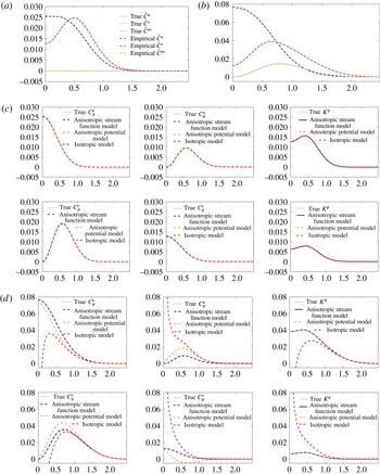
We generate sample paths of the underlying Gaussian process and use both the anisotropic stream function model and the isotropic model for the decomposition. The one-dimensional spectra are shown in figure 3(a), indicating a negligible sampling error. As we can see in figure 3(c), both models recover the true decomposition with small and comparable error. The fact that the anisotropic stream function model matches the isotropic model is guaranteed by (5.2) together with
 $\mathbb{E}u^{2}=\mathbb{E}v^{2}$
.
Synthetic data Examples 1 in (5.3) and 2 in (5.4)–(5.5). (a) + (b) Observed one-dimensional spectra. (c) + (d) Helmholtz decomposition using different models. Note divergence of the isotropic model in red when applied to anisotropic data. (a) Isotropic spectra Example 1. (b) Anisotropic spectra Example 2. (c) Decomposition of isotropic spectra Example 1. (d) Decomposition of anisotropic spectra Example 2.

Example 2. We now assume that there is anisotropy, but only in the stream function component:
 $$\begin{eqnarray}\displaystyle {\hat{C}}^{\unicode[STIX]{x1D713}}(k,l) & = & \displaystyle \exp (-\unicode[STIX]{x03C0}k_{h}^{2})+(k\cos (2\unicode[STIX]{x03C0}/3)+l\sin (2\unicode[STIX]{x03C0}/3))^{2}\exp \left(-\frac{\unicode[STIX]{x03C0}}{2}k_{h}^{2}\right),\end{eqnarray}$$
 $$\begin{eqnarray}\displaystyle {\hat{C}}^{\unicode[STIX]{x1D719}}(k,l) & = & \displaystyle {\textstyle \frac{1}{2}}\exp (-\unicode[STIX]{x03C0}k_{h}^{2}).\end{eqnarray}$$
With
 $\unicode[STIX]{x1D703}=2\unicode[STIX]{x03C0}/3$
in the second quadrant we expect
 $\mathbb{E}uv>0$
, as is confirmed by the one-dimensional spectra shown in figure 3(b). When both the isotropic and anisotropic stream function model are applied, the isotropic model is unable to capture the anisotropy, generating significant model error. This includes divergent values for some of the spectra in figure 3(d). On the other hand, the anisotropic stream model, which has the correct model assumptions, successfully recovers the true decomposition. Notably, in this example
 $\mathbb{E}u^{2}>\mathbb{E}v^{2}$
and the true
 $K^{\unicode[STIX]{x1D713}}$
in figure 3(d) is indeed larger than its isotropic counterpart, in accordance with (4.7).
We have also used this example to probe spectra in the limit
 $\unicode[STIX]{x1D703}\rightarrow 0$
, which is the Achilles heel case of our method, i.e.
 $\mathbb{E}uv=0$
but
 $\mathbb{E}u^{2}-v^{2}\neq 0$
. We found that our method works well down to
 $\unicode[STIX]{x1D703}\approx 0.1$
, but not below that.
Example 3. Our third example is
 $$\begin{eqnarray}{\hat{C}}^{\unicode[STIX]{x1D713}}(k,l)=\exp (-2\unicode[STIX]{x03C0}(k^{2}+3l^{2}+2kl))\quad \text{and}\quad {\hat{C}}^{\unicode[STIX]{x1D719}}(k,l)=0.\end{eqnarray}$$
The rotational spectrum is anisotropic, with non-zero
 $\mathbb{E}uv>0$
and
 $\mathbb{E}u^{2}-v^{2}<0$
, but it is not of the form assumed in our models! Moreover, the divergent spectrum is precisely zero, signalling an absence of any internal wave motion in the linear wave–vortex decomposition scheme described in § 4, which is an additional challenge for the models to get right. This severely tests the robust performance of our models in realistic settings.
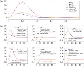
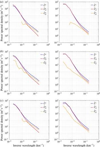
The outcome is depicted in figure 4, which shows that the only credible choice here is the anisotropic stream function model (3.17). That model manages to recover the true decomposition of the spectra reasonably well and it captures the dominance of the rotational kinetic energy. In contrast, the isotropic model yields divergent spectra as in the previous example whilst the anisotropic potential model produces significant negative values of
 ${\hat{C}}_{\unicode[STIX]{x1D719}}^{u}$
, which are clearly unphysical. We consider the ability of our models to predict their own breakdown by producing unphysical results a positive feature of our method. As always, the kinetic energy spectra of the anisotropic models are identical, and here they recover the true decomposition remarkably well.

Example 4. Our final example is the most challenging:
 $$\begin{eqnarray}\displaystyle & \displaystyle {\hat{C}}^{\unicode[STIX]{x1D713}}(k,l)=\left\{\begin{array}{@{}ll@{}}\exp (-2\unicode[STIX]{x03C0}(k^{2}+3l^{2}+2kl)),\quad & k_{h}<0.6,\\ 2\exp (-2\unicode[STIX]{x03C0}k_{h}^{2}),\quad & k_{h}\geqslant 0.6,\end{array}\right. & \displaystyle\end{eqnarray}$$
 $$\begin{eqnarray}\displaystyle & \displaystyle {\hat{C}}^{\unicode[STIX]{x1D719}}(k,l)=\exp (-2\unicode[STIX]{x03C0}(k^{2}+2l^{2}+kl)). & \displaystyle\end{eqnarray}$$
Here both
 $\unicode[STIX]{x1D713}$
and
 $\unicode[STIX]{x1D719}$
feature different kinds of anisotropies, but neither conforms to our model. Moreover, the stream function spectrum has a discontinuity and its anisotropy is restricted to a finite wavenumber range as indicated, which mimics a return to isotropy at small scales. As expected, figure 5 shows that the decomposition of the individual velocity components is poor for all models in this example, but we nonetheless recover extremely good results for the Helmholtz decomposition of the kinetic energy based on the new anisotropic method! We feel that this bodes well for a robust wave–vortex decomposition in practical settings.
5.3 Analysis of Gulf Stream data
In this section we apply the anisotropic Helmholtz decomposition to Gulf Stream spectra from the Oleander dataset (Flagg et al. Reference Flagg, Schwartze, Gottlieb and Rossby1998), which was previously analysed using the isotropic Helmholtz and wave–vortex decomposition in BCF14. We chose this dataset as a convenient first test case because it is easily available, has been analysed using isotropic methods several times before, and can be expected to have noticeable anisotropic components due to the vicinity of the Gulf Stream.
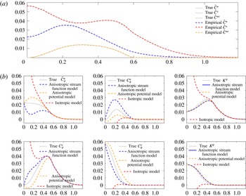
Example 4 using (5.7)–(5.8), with strong anisotropies in both
 $\unicode[STIX]{x1D713}$
and
 $\unicode[STIX]{x1D719}$
that do not conform to the assumptions of our method. The lower panels show that the method cannot reliably decompose the individual velocity components, but that the anisotropic method does remarkably well for the crucial Helmholtz decomposition of the kinetic energy. (a) Anisotropic spectra Example 4. Note that
 ${\hat{C}}^{uv}=0$
for
 $k>0.6$
. (b) Decomposition of anisotropic spectra Example 4.

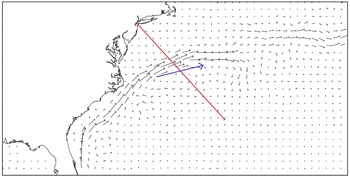
The Oleander Project collected velocity data from tracks between New York Harbour and Bermuda (see figure 6). Our data processing steps are standard and follow those in Callies & Ferrari (Reference Callies and Ferrari2013) and BCF14. We used velocity observations at
 $150$
m depth collected between 1994 and 2004. We removed those tracks that were too far away from a geodesic by measuring the
 $L_{2}$
distance between tracks. We also removed those tracks that had too large gaps between observations. After this filtering, we were still left with
 $397$
ship tracks, from which we interpolated the velocity observations onto an equally spaced grid of
 $2.5$
km. We removed the average velocity from each ship track, calculated the spectra of each ship track, and took the average among tracks as a surrogate for taking the expectation.
Sketch of geographical location of the Oleander dataset and typical Gulf Stream current structure; typical current speeds are of the order of one metre per second. The ship track is indicated in red and the diagnosed first principal direction of the velocity field is indicated in blue. The diagnosed velocity fields are eddy fields, i.e. all velocity measurements along the ship track have their mean value removed, ensuring that
 $\mathbb{E}u=\mathbb{E}v=0$
(cf. Callies & Ferrari (Reference Callies and Ferrari2013) and BCF14.)

The data are known from previous studies to be dominated by vortical flow rather than inertia–gravity waves over most of their scale range, which is not too surprising given the vicinity of the Gulf Stream. Hence, one can anticipate that as the dataset is dominated by the stream function component over the potential flow component, that this will also be true for the anisotropic component. For comparison purposes, however, we run all three possible models and let the results speak for themselves.
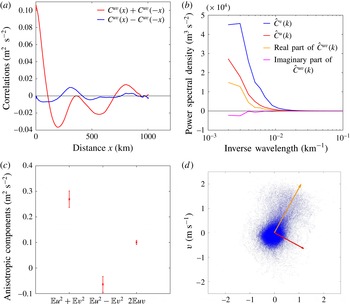
Gulf Stream data. (a) Odd and even components of
 $C^{uv}(x)$
. (b) Corresponding real and imaginary part of
 ${\hat{C}}^{uv}(k)$
. (c) Observed statistics
 $\mathbb{E}u^{2}+\mathbb{E}v^{2}$
,
 $\mathbb{E}u^{2}-\mathbb{E}v^{2}$
and
 $2\mathbb{E}uv$
with error bar of 95 % confidence interval. (d) Observed
 $(u,v)$
velocity samples from ship tracks from 1994 to 2004. The orange and red arrows are the first and second principal directions of the velocity field and correspond to
 $\unicode[STIX]{x1D6FE}$
and
 $\unicode[STIX]{x1D703}$
, respectively.

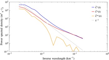
Energy spectra and cross-spectrum from the Gulf Stream: observed transverse and longitudinal kinetic energy spectra
 ${\hat{C}}^{u}$
,
 ${\hat{C}}^{v}$
and cross-spectra
 ${\hat{C}}^{uv}$
. A line corresponding to a
 $k^{-3}$
power law has also been added for reference.

Helmholtz decomposition of Gulf Stream data. The left side shows the longitudinal spectrum
 ${\hat{C}}^{u}$
and the right side shows the transverse spectrum
 ${\hat{C}}^{v}$
. Shown are the results of the (a) isotropic, (b) anisotropic stream and (c) anisotropic potential model. Missing parts in these log–log plots indicate negative values.

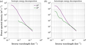
Helmholtz decomposition of the kinetic energy spectrum for the Gulf Stream data. (a) Shows the isotropic model (as in BCF14) and (b) shows the new anisotropic model, which recovers significantly more of the divergent spectrum
 $K^{\unicode[STIX]{x1D719}}$
at large scales. This indicates the anisotropy of the data at large scales.

We first computed the quantities
 $\mathbb{E}u^{2}-\mathbb{E}v^{2}$
and
 $\mathbb{E}uv$
from the raw data as shown in figure 7(b). These are clearly non-zero, with
 $\mathbb{E}u^{2}-\mathbb{E}v^{2}<0$
and
 $\mathbb{E}uv>0$
, and therefore indicate an anisotropic component. In figure 7(c) the corresponding principal directions of the random velocity field are indicated by arrows, with the orange line corresponding
 $\unicode[STIX]{x1D703}$
and the red line corresponding to
 $\unicode[STIX]{x1D6FE}$
. Also plotted in figure 7(a) are the even and odd parts of the cross-correlation function
 $C^{uv}(x)$
, which indicates a non-zero odd part but also that this part is much smaller than the even part. The corresponding statement applies to the spectrum
 ${\hat{C}}^{uv}(k)$
plotted in figure 8, which has a dominant real part and a weaker imaginary part, at least for the lower to middle range of wavenumbers. Importantly, the real part of
 ${\hat{C}}^{uv}(k)$
is sign-definite across the scales, although at large wavenumbers the spectrum becomes noisy. Still, this indicates that the velocity cross-correlation can be approximated by a single anisotropy direction for all scales, which is an intrinsic feature of our models. Performing our model selection algorithm on the data, we hence find that the test for the assumption of independence between the stream and potential functions is passed at a reasonable level.
The observed
 ${\hat{C}}^{u}$
and
 ${\hat{C}}^{v}$
are shown in figure 8, both have a
 $k^{-3}$
decay in the large scales. There is however a flattening starting around a wavelength of
 $50$
km, a phenomenon that could be related to the numerical algorithm used to compute the spectra. The Helmholtz decomposition of the Gulf Stream spectra following each model are shown on figure 9. While the three models give similar decomposition at small scales (
 $k^{-1}<20~\text{km}$
), at a relatively larger scale (
 $k^{-1}>100~\text{km}$
), both the isotropic model and the anisotropic potential model give negative spectra, which can be attributed to the non-satisfaction by the data of these models’ assumptions. On the other hand, the anisotropic stream function model decomposes the spectra into physically meaningful, positive spectra at all wavelengths, which we take to indicate that it is the most consistent with the Gulf Stream data. The energy components
 $K^{\unicode[STIX]{x1D713}}$
and
 $K^{\unicode[STIX]{x1D719}}$
are dominant at different scales (figure 10): for wavelengths larger then 50 km, the stream component dominates, while at smaller scales (
 $k^{-1}<20~\text{km}$
) the potential component contributes most to the kinetic energy. As a reminder, the stream components
 $K^{\unicode[STIX]{x1D719}}$
corresponds to the half of the total wave energy
 $\mathbb{E}_{W}$
. Since no buoyancy data are available in this dataset, the vortical component of the energy cannot be recovered. However, it is clear that at large scales, where
 $K^{\unicode[STIX]{x1D719}}$
is substantially smaller than
 $K^{\unicode[STIX]{x1D713}}$
, the vortical component contributes most to the energy spectra. Notably, the anisotropic model is able to recover the
 $K^{\unicode[STIX]{x1D719}}$
spectrum over a much larger range than is possible with the isotropic model, which is an advantage. For example, this means that the prediction of wave energy levels is possible over a wider range of scales in the anisotropic model. Overall, we consider this an encouraging first test run with real ocean data.
6 Concluding remarks
In this paper we have developed and tested a simple anisotropic extension of the isotropic Helmholtz and wave–vortex decomposition method for one-dimensional spectra presented in BCF14. Under appropriate modelling choices both velocity components can be decomposed into rotational and divergent parts, but the most important results are the Helmholtz decomposition of the kinetic energy in (3.30)–(3.31) and the accompanying expression for the wave energy in (4.6):
 $$\begin{eqnarray}\displaystyle & \displaystyle 2K^{\unicode[STIX]{x1D713}}(k)={\hat{C}}^{v}(k)+\frac{1}{k}\int _{k}^{\infty }\left[{\hat{C}}^{v}(\bar{k})-{\hat{C}}^{u}(\bar{k})+\frac{\mathbb{E}u^{2}-\mathbb{E}v^{2}}{\mathbb{E}uv}{\hat{C}}^{uv}(\bar{k})\right]\,\text{d}\bar{k}, & \displaystyle\end{eqnarray}$$
 $$\begin{eqnarray}\displaystyle & \displaystyle 2K^{\unicode[STIX]{x1D719}}(k)={\hat{C}}^{u}(k)-\frac{1}{k}\int _{k}^{\infty }\left[{\hat{C}}^{v}(\bar{k})-{\hat{C}}^{u}(\bar{k})+\frac{\mathbb{E}u^{2}-\mathbb{E}v^{2}}{\mathbb{E}uv}{\hat{C}}^{uv}(\bar{k})\right]\,\text{d}\bar{k}, & \displaystyle\end{eqnarray}$$
 $$\begin{eqnarray}\displaystyle & \displaystyle E_{W}(k)=2K^{\unicode[STIX]{x1D719}}(k)+{\hat{C}}^{w}(k). & \displaystyle\end{eqnarray}$$
These expressions do not require any particular modelling choice and can be used ‘as is’ for data analysis, except in the Achilles heel case (1.4), in which one must revert to the isotropic version.
Compared to the isotropic method in BCF14, the new ingredient is the one-dimensional cross-spectrum
 ${\hat{C}}^{uv}$
, which can be computed from the raw
 $(u,v)$
-data just as
 ${\hat{C}}^{u}$
and
 ${\hat{C}}^{v}$
. So this new ingredient requires no new data sources. Moreover, it is obvious from these equations that the new method also requires no extra computational cost and we have demonstrated that it reliably reduces to the isotropic method in the appropriate limit. Overall, we found the method robust and easy to use and we hope that it will be as useful in practice as its isotropic progenitor.
Of course, as discussed, any anisotropic extension can only work by restricting the class of possible anisotropies in some fashion, so there is a balancing act between the requirement to have a simple tractable model and the desire to cover the greatest possible class of anisotropies that may occur in nature. One physical limitation of our method is that the anisotropy direction
 $\unicode[STIX]{x1D703}$
or
 $\unicode[STIX]{x1D6FE}$
is assumed to be the same for all wavenumbers
 $k$
; being able to relax this assumption would be a considerable advantage. Another limitation is that the observed cross-spectrum
 ${\hat{C}}^{uv}(k)$
has to be real and sign-definite, which can lead to practical problems with noisy spectra, especially at large wavenumber
 $k$
. Here a pragmatic solution is to just use the real part of the observed
 ${\hat{C}}^{uv}(k)$
, or even to use the absolute value
 $|{\hat{C}}^{uv}(k)|$
instead. For what it is worth, we have tested these variations on the ocean data in this paper and found no significant changes.
Also, one might investigate specific physical conditions that would lead to an imaginary part of
 ${\hat{C}}^{uv}(k)$
, which we know implies a statistical correlation between
 $\unicode[STIX]{x1D713}$
and
 $\unicode[STIX]{x1D719}$
. Such an investigation might also lead to further improvements already in the isotropic case. A natural candidate in this direction is to consider the ageostrophic corrections to quasi-geostrophic dynamics, which involve a flow potential
 $\unicode[STIX]{x1D719}$
that is slaved to the quasi-geostrophic stream function
 $\unicode[STIX]{x1D713}$
. Conversely, it would be interesting to consider nonlinear corrections to the internal wave field and how they would affect the wave–vortex decomposition method. This should be approachable at least for weakly nonlinear waves, or in regimes such as the one studied in Young & Jelloul (Reference Young and Jelloul1997).
Finally, it would be desirable to find a way to avoid the Achilles heel case (1.4), which may never occur in practice, but mars the otherwise clean appearance of our method.
Acknowledgements
Fruitful discussions with J. Callies, R. Ferrari and F. Zhang are gratefully acknowledged. The constructive and critical comments of three referees greatly helped to improve the manuscript. Financial support was provided under grants DMS-1312159 and DMS-1516324 of the US National Science Foundation and under grant N00014-15-1-2355 of the US Office of Naval Research.
Appendix A. Manipulations of correlation functions
We illustrate how to manipulate two-dimensional correlation functions such as
 $$\begin{eqnarray}C_{\unicode[STIX]{x1D713}}^{uv}(x,y)=-\mathbb{E}[\unicode[STIX]{x1D713}_{y}(x_{0},y_{0})\unicode[STIX]{x1D713}_{x}(x_{0}+x,y_{0}+y)].\end{eqnarray}$$
The key is consider the quantity in square brackets temporarily as a function of the four independent variables
 $(x_{0},y_{0},x,y)$
and to exploit the fact that the expectation of any quantity is independent of
 $(x_{0},y_{0})$
by the assumption of homogeneity. This results in
 $$\begin{eqnarray}\displaystyle C_{\unicode[STIX]{x1D713}}^{uv}(x,y) & = & \displaystyle -\mathbb{E}\left[\frac{\unicode[STIX]{x2202}}{\unicode[STIX]{x2202}y_{0}}(\unicode[STIX]{x1D713}(x_{0},y_{0}))\frac{\unicode[STIX]{x2202}}{\unicode[STIX]{x2202}x}\unicode[STIX]{x1D713}(x_{0}+x,y_{0}+y)\right]\nonumber\\ \displaystyle & = & \displaystyle +\frac{\unicode[STIX]{x2202}}{\unicode[STIX]{x2202}x}\mathbb{E}\left[\unicode[STIX]{x1D713}(x_{0},y_{0})\frac{\unicode[STIX]{x2202}}{\unicode[STIX]{x2202}y_{0}}\unicode[STIX]{x1D713}(x_{0}+x,y_{0}+y)\right]\nonumber\\ \displaystyle & = & \displaystyle +\frac{\unicode[STIX]{x2202}}{\unicode[STIX]{x2202}x}\mathbb{E}\left[\unicode[STIX]{x1D713}(x_{0},y_{0})\frac{\unicode[STIX]{x2202}}{\unicode[STIX]{x2202}y}\unicode[STIX]{x1D713}(x_{0}+x,y_{0}+y)\right]\nonumber\\ \displaystyle & = & \displaystyle +\frac{\unicode[STIX]{x2202}^{2}}{\unicode[STIX]{x2202}x\unicode[STIX]{x2202}y}\mathbb{E}[\unicode[STIX]{x1D713}(x_{0},y_{0})\unicode[STIX]{x1D713}(x_{0}+x,y_{0}+y)]\nonumber\\ \displaystyle & = & \displaystyle \frac{\unicode[STIX]{x2202}^{2}}{\unicode[STIX]{x2202}x\unicode[STIX]{x2202}y}C^{\unicode[STIX]{x1D713}}(x,y).\end{eqnarray}$$
For the power spectra this is equivalent to
 $$\begin{eqnarray}{\hat{C}}_{\unicode[STIX]{x1D713}}^{uv}(k,l)=-kl{\hat{C}}^{\unicode[STIX]{x1D713}}(k,l),\end{eqnarray}$$
which is listed in (2.5). The other expressions are derived in the same way.