2 Preliminaries

The set of nonnegative integers is ℕ, and we let [n] = {i ∈ ℕ | 1 ≤ i ≤ n} for every n ∈ ℕ. An alphabet is a finite set Σ of symbols. The set of all strings over Σ is Σ*, of which the empty string is ϵ. Concatenation of strings is denoted by juxtaposition. For each w ∈ Σ*, the length |w| of w is the number of occurrences of symbols in w. The ith letter in w with 1 ≤ i ≤ |w| is denoted by w _i.

A commutative semiring (Hebisch and Weinert Reference Hebisch and Weinert1998; Golan Reference Golan1999) is an algebraic structure (A, +, ⋅, 0, 1) such that

• • (A, +, 0) and (A, ⋅, 1) are commutative monoids, and

• • the multiplication ⋅ distributes over finite sums (in particular, a ⋅ 0 = 0 = 0 ⋅ a for every a ∈ A).

Examples of commutative semirings are

• • the real number semiring (ℝ, +, ⋅, 0, 1),

• • the Boolean semiring ({0, 1}, max, min, 0, 1), and

• • the tropical semiring (ℕ ∪ {∞}, min, +, ∞, 0).

In addition, every commutative field or ring is a commutative semiring.

In the rest of the paper, let (A, +, ⋅, 0, 1) be a commutative semiring. For every mapping f : S → A, we let supp(f) = {s ∈ S | f(s) ≠ 0} be the support of f. As usual, we write Σ_{s ∈ S}f(s) for the sum of the elements f(s) for every s ∈ S provided that supp(f) is finite. We also write ∏_s∈Sf(s) for the product of the elements f(s) for every s ∈ S provided that S is finite.

A weighted string automaton (wsa) (Schützenberger Reference Schützenberger1961; Eilenberg Reference Eilenberg1974) is a system N = (P, Γ, J, ν, G), where

• • P and Γ are alphabets of states and input symbols, respectively,

• • J, G: P → A assign initial and final weights, respectively, and

• • ν : P × Γ × P → A assigns a weight to each transition.

Let w = γ₁ ⋅⋅⋅ γ_k ∈ Γ* be an input string with γ_i ∈ Γ for every i ∈ [k]. Every mapping r: [k+1] → P is a run on w. The set of all runs on w is denoted by Run _N(w), and we write r _i instead of r(i) for every r ∈ Run _N(w) and i ∈ [k+1]. The weight wt _N(r) of the run r ∈ Run _N(w) is ∏_{i = 1}^k ν(r _i, γ_i, r _i+1). Finally, the semantics of the wsaN assigns to w the weight

A good introduction to wsa can be found in Mohri (Reference Mohri, Droste, Kuich and Vogler2009) or Sakarovitch (Reference Sakarovitch, Droste, Kuich and Vogler2009).

A ranked alphabet Σ = ⋃_k∈ℕ Σ_k is an alphabet whose symbols have assigned ranks. Contrary to some of the standard literature, we do not assume that each symbol of a ranked alphabet has only one fixed rank. For every k ∈ ℕ, the set Σ_k contains all symbols of rank k. For a given set T, we let Σ(T) = {σ(t ₁,. . .,t _k) | σ ∈ Σ_k, t ₁,. . .,t _k ∈ T). The set T _Σ(V) of Σ-trees indexed by a set V is the smallest set T such that V ⊆ T and Σ(T) ⊆ T. For every t ∈ T _Σ(V) and S ⊆ Σ ∪ V, let pos _S(t) ⊆ ℕ* be the set of positions labeled by elements of S. Formally, for every v ∈ V, σ ∈ Σ_k, and t ₁,. . .,t _k ∈ T _Σ(V)

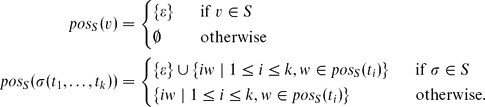
Clearly, positions are lexicographically ordered. We denote this order simply by ≤. Moreover, let |t|_S = |pos _S(t| be the number of occurrences of symbols of S in t. If S = {s}, then we write pos _s(t) and |t|_s instead of pos _S(t) and |t _S, respectively. The positions pos(t) and the size |t| are pos _Σ∪V(t) and |t|_Σ∪V), respectively. Moreover, let var(t) = {v ∈ V | pos _v(t) ≠ ∅}. A tree t ∈T _Σ(V) is linear in V if |pos _v(t)| ≤ 1 for every (v ∈ V.

Let S ⊆ Σ₀ ∪ V. The S-yield yd _S(t) of a tree t ∈ T _Σ(V) is recursively defined as follows:

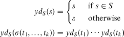
for every s ∈ Σ₀ ∪ V, σ ∈ Σ_k with k > 1, and t ₁,. . .,t _k ∈ T _Σ(V). If S = Σ₀ ∪ V, then we simply write yd(t) instead of yd _S(t).

Let ◻ be a distinguished symbol that has only the rank 0. Let Δ be the ranked alphabet such that Δ₀ = Σ₀ ∪ {◻} and Δ_k = Σ_k for every k ≥ 1. A Σ-context c indexed by V is a tree of T _Δ(V) such that |c|_◻ = 1. The set of all Σ-contexts indexed by V is C _Σ(V). The tree c[t] is obtained from c by replacing the symbol ◻ by t. More generally, t[u]_w denotes the result of replacing the subtree at position w ∈ pos(t) in t ∈ T _Σ(V) by the tree u ∈ T _Σ(V). In particular, c[t] = c[t]_w where w is the unique element in pos _◻(c). Finally, any mapping θ: V′ → T _Σ(V) with V′ ⊆ V is a substitution. The application tθ of the substitution θ to a tree t ∈ T _Σ(V) is defined by

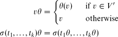
for every v ∈ V, σ ∈ Σ_k, and t ₁,. . .,t _k ∈ T _Σ(V). We often use elements of the fixed set X = {x ₁, x ₂,. . .} of (formal) variables as substitution variables. If we write x _i, then we implicitly assume that i ≥ 1. A tree t ∈ T _Σ(X) is k-normed if yd _X(t) = x ₁ ⋅⋅⋅x _k. Given t ∈ T _Σ, we let

which is finite.

A weighted synchronous tree substitution grammar (stsg) (Chiang and Knight (Reference Chiang, Knight, Calzolari, Cardie and Isabelle2006) is a system M = (Q, Σ, Δ, I, R) where

• • Q is an alphabet of nonterminals such that Q ∩ (Σ ∪ Δ) = ∅,

• • Σ and Δ are ranked alphabets of input and output symbols, respectively,

• • I : Q → A assigns initial weights, and

• • R : T _Σ(Q) × Q × T _Δ(Q) → A are weighted rules such that supp(R) is finite and for every (t, q, u) ∈ supp(R)

  • — t and u are linear in Q,

  • — var(t) = var(u), and

  • — t ∉ Q or u ∉ Q.

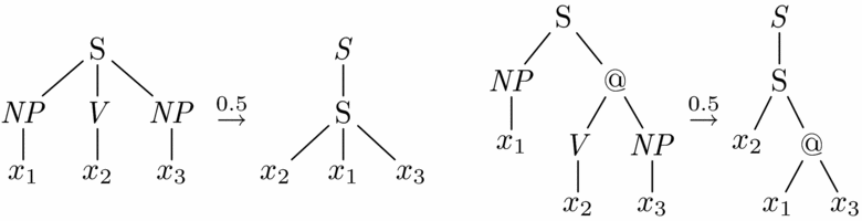
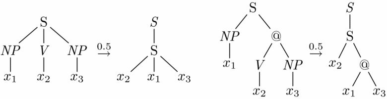
In a rule (t, q, u) ∈ supp(R), the tree t is the left-hand side, q is the target state, and u is the right-hand side. The first two restrictions on rules ensure that exactly the same states occur in t and u. Moreover, no state is allowed to occur twice in the left- or right-hand side. Intuitively, the links between the states are implicit by the assumption that equal states in the left- and right-hand side are linked. A sample stsg rule is displayed in Figure 1, where the nonterminals are slanted, and we assume that the root terminal is also the nonterminal.

Fig. 1.

stsg rule and the same rule with binarized trees where @ is an arbitrary symbol that is introduced in the binarization process. We could (without harm) add another @-symbol to represent the children of S in a list.

The distinction between nonterminals and terminals is uncommon for stsg (Chiang Reference Chiang, Knight, Ng and Oflazer2005), but it increases the generative power. Our stsg are equivalent to the (nondeleting and linear) extended top-down tree transducers of Graehl et al. (Reference Graehl, Knight and May2008) and Maletti et al. (Reference Maletti, Graehl, Hopkins and Knight2009). The size |(t, q, u)| of a rule (t, q, u) ∈ supp(R) is |t| + |u|, and the size |M| of the stsg |M| is Σ_ρ∈supp(R)|ρ|. The stsgM is a weighted synchronous context-free grammar (scfg) if t ∈ Σ(Q) and u ∈ Δ(Q) for every rule (t, q, u) ∈ supp(R). Finally, M is a weighted tree substitution grammar (tsg) if t = u for all rules (t, q, u) ∈ supp(R). A detailed exposition to stsg, scfg, and tsg can be found in Chiang (Reference Chiang, Knight, Ng and Oflazer2005), Berstel and Reutenauer (Reference Berstel and Reutenauer1982), or Fülöp and Vogler (Reference Fülöp, Vogler, Droste, Kuich and Vogler2009).

Let us proceed with the semantics of an stsgM = (Q, Σ, Δ, I, R). Equal nonterminals in t and u of a rule (t, q, u) ∈ supp(R) are linked. Those links need to be remembered in sentential forms. Given t ∈ T _Σ(Q), u ∈ T _Δ(Q), and ℓ : pos _Q(t) → pos _Q(u), the triple (t, ℓ, u) is a sentential form if

• • ℓ is a bijection and

• • ℓ(w) ∈ pos _q(u) for every q ∈ Q and w ∈ pos _q(t).

In other words, ℓ is a bijection that respects the nonterminals. Given two sentential forms ξ = (t ₁, ℓ₁, u ₁) and (ζ = (t ₂, ℓ₂, u ₂), we write if there is a rule (t, q, u) ∈ supp(R) such that

• • t ₁ = t ₁[q]_{w 1} and u ₁ = u ₁[q]_{w 2},

• • t ₂ = t ₁[t]_{w 1} and u ₂ = u ₁[u]_{w 2},

• • a = R(t, q, u), and

• • ℓ₂ = (ℓ₁ ∖ {(w ₁, w ₂)}) ∪ {(w ₁w′, w _2w″)|q ∈ Q, w′ ∈ pos _q(t), w″ ∈ pos _q(u)},

where w ₁ = min(pos _Q(t ₁)) and w ₂ = ℓ₁(w ₁). The selection of the minimal state-labeled position in t ₁ ensures that we obtain a left-most derivation with respect to the input side. A sequence D = (ξ,. . .,ξk) of sentential forms is a derivation if there exist a ₁,. . .,a _k ∈ A such that for every i ∈ [k]). Note that if such weights a ₁,. . .,a _k exist, then they are unique. Consequently, we define the weight wt _M(D) of the derivation D to be . Moreover, for every q ∈ Q and sentential form ζ = (t, ℓ, u) we let

Note that the set D _M^q(ζ) is finite because each derivation step creates an input or an output symbol by the final condition on rules in the definition of stsg. The q-weight M _q(ζ) assigned by the stsgM to ζ is and for every t ∈ T _Σ and u ∈ T _Δ.

For a tsgM = (Q, Σ, Σ, F, R), we will simply write R(q → t) instead of R(t, q, t) for every q ∈ Q and t ∈ T_ _Σ(Q). Moreover, we write M _q(t) and (M(t) instead of M _q(t, ∅, t) and M(t, t) for every q ∈ Q and t ∈ T _Σ. Finally, we drop the linearity requirement for tsg; i.e., t need not be linear in Q for a rule (q → t) ∈ supp(R). A mapping ϕ : T _Σ → A is recognizable (Fülöp and Vogler Reference Fülöp, Vogler, Droste, Kuich and Vogler2009) if there exists a tsgN such that ϕ = N. The following proposition is well-known (Alexandrakis and Bozapalidis Reference Alexandrakis and Bozapalidis1987).

Proposition 1

For every tsg there exists an equivalent tsg that is also a scfg.

While the derivation semantics of an stsgM = (Q, Σ, Δ, I, R) is very instructive, it is difficult to handle in formal proofs. We observe the following equality:

for every q ∈ Q, t ∈ T _Σ, and u ∈ T _Δ. Note that we will write M _q(t, ∅, u) instead of M _q(t, u) if t ∈ T _Σ. This equality can also be used as a recursive definition of M _q(t, u) because the recursive calls M _p(pθ, pθ′) are made to smaller trees (i.e., |pθ| ≤ |t| and |pθ′| ≤ |u| and one of these inequalities is strict) since t′ ∉ Q or u′ ∉ Q. Let us prove this equality. Note that we essentially separate the first derivation step, which is typical for top-down devices.

3 Multi bottom-up tree transducers

We already mentioned in the Introduction that we want to compare stsg to another model that we propose as an alternative. The alternative is the weighted (linear and nondeleting) multi bottom-up tree transducer, which has been introduced by Arnold and Dauchet (Reference Arnold and Dauchet1982) and Lilin (Reference Lilin, Astesiano and Böhm1981). A more detailed (and English) presentation is Engelfriet et al. (Reference Engelfriet, Lilin and Maletti2009). Let us quickly recall the formal definition, which we extend with weights. Recall that X = {x ₁, x ₂, . . .}.

Definition 2

A weighted multi bottom-up tree transducer (mbot) is a system (Q, Σ, Δ, F, R) where

• • Q, Σ, and Δ are ranked alphabets of states, input symbols, and output symbols, respectively,

• • F : Q ₁ → A assigns final weights to unary states Q ₁, and

• • R : T _Σ(Q(X)) × Q(T _Δ(X)) → A are weighted rules such that supp(R) is finite and for every (l, r) ∈ supp(R)

  • — l and r are linear in X,

  • — var(l) = var(r), and

  • — l ∉ Q(X) or r ∉ Q(X).

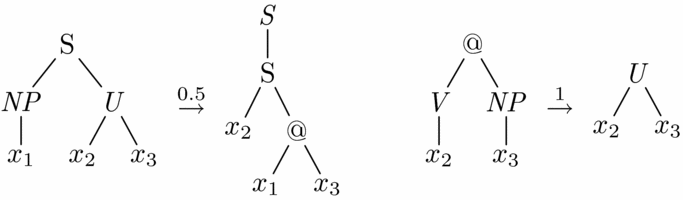
The components l and r of a rule (l, r) ∈ supp(R) are called left- and right-hand side, respectively. Although we will not use a linking structure for mbot, the links can be imagined between equal variables of X (not between the symbols of Q) in the left- and right-hand side of a rule. Figure 2 displays example rules of an mbot. Roughly speaking, an mbot is a weighted (linear and nondeleting) extended bottom-up tree transducer (Engelfriet, Fülöp and Vogler Reference Engelfriet, Fülöp and Vogler2002; Engelfriet, Lilin and Maletti Reference Engelfriet, Lilin and Maletti2009), in which the states of Q can have ranks different from 1. To keep the presentation simple, we assume that final states have rank 1 (hence the final weight assignment F is of type F : Q ₁ → A). The size |(l, r)| of a rule (l, r) ∈ supp(R) is |l| + |r|, and the size |M| of the mbotM is Σ_ρ∈supp(R) |ρ|.

Fig. 2.

mbot rule (states are slanted) and the same rule with binarized trees where @ is an arbitrary symbol that is introduced in the binarization process.

The final condition on the rules in Definition 2 ensures that derivations are finite because each step will consume an input symbol or generate an output symbol. We continue with the rewrite semantics for the mbotM = (Q, Σ, Δ, F, R). Again, we define left-most derivations only.

Definition 3

Let c ∈ C _Σ(Q(T _Δ)) and θ : X → T _Δ such that w < w′ for every w ∈ pos _◻(c) and w′ ∈ pos _Q(c). Then if R(l, r) = a). A sequence D = (ξ₀,. . .,ξ_k) of ξ_i ∈ T _Σ(Q(T _Δ)) is a derivation if there are a ₁,. . .,a _k ∈ A such that . Note that such weights a ₁,. . .,a _k are unique. The weight wt _M(D) of the derivation D is . Moreover, for every ξ, ζ ∈ T _Σ(Q(T _Δ)), we let

Note that the set D _M(ξ, ζ) is finite. For every t ∈ T _Σ, and r′ ∈ Q(T _Δ), let . The weight M(t, u) assigned by the mbotM is M(t, u) = Σ_{q∈Q 1}F(q)⋅M(t, q(u)) for every t ∈ T _Σ and u ∈ T _Δ.

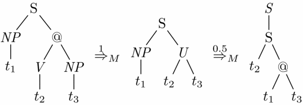
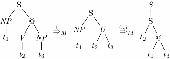
Note that the condition on the context c in Definition 3 ensures that the derivation is left-most. The rules of Figure 3 are applied in a derivation in Figure 4. The first displayed derivation step uses the context S(NP(t ₁), ◻) and any substitution θ such that θ(x ₂) = t ₂ and θ(x ₃) = t ₃.

Fig. 3.

Sample mbot rules in one-symbol normal form (see Definition 5; in essence each rule contains exactly one input or output symbol). The states of Q are slanted.

Fig. 4.

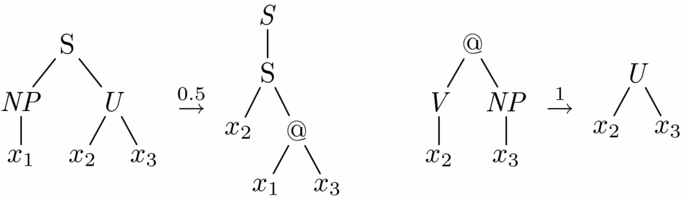
Derivation using the mbot rules of Figure 3.

Again, the derivation semantics is very instructive, but difficult to handle in proofs. To overcome this problem, we observe the following equality:

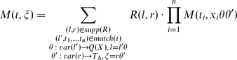
for every t ∈ T _Σ and ξ ∈ Q(T _Δ). Again, this equation also yields a recursive definition of M(t, ξ) because the recursive calls are made to smaller input or output trees.

Again, let us prove this equality, so that we have a solid base for the following proofs. For every t ∈ T _Σ and ξ ∈ Q(T _Δ),

This proof is similar to the corresponding proof for stsg, but here we separated the last derivation step, which is common for bottom-up devices.

It is argued by Chiang (Reference Chiang, Knight, Ng and Oflazer2005), Knight (Reference Knight2007), and Graehl et al. (Reference Graehl, Knight and May2008) that stsg (and extended top-down tree transducers) have sufficient power for syntax-based machine translation. mbot should be at least as powerful as stsg, we first demonstrate how each stsg can be encoded as an mbot.

Theorem 4

For every stsgM, we can construct an equivalent mbot in time (|M|).

Proof

Let M = Q, Σ, Δ, I, R) be an stsg. Then we construct the mbotM′ = (Q′, Σ, Δ, I, R′) with Q′₁ = Q and Q′_k = ∅ for every k ≠ 1 and for every (t, q, u) ∈ supp(R) we let R′(l, r) = R(t, q, u) where

• • var(t) = {q ₁,. . .,q _k},

• • and with and for every i ∈ [k], and

• • l = tθ_{q 1. . .q k} and r = q(uθ′_{q 1. . .q k}).

Clearly, M′ can be constructed in time (|M|). To prove the correctness of the construction, we have to prove the statement M _q(t′, u′) = M′(t′, q(u′)) for every q ∈ Q, t′ ∈ T _Σ, and u′ ∈ T _Δ.

With this auxiliary statement, the main statement is now easy to prove for every t ∈ T _Σ and u ∈ T _Δ.

□ stsg rules and their corresponding mbot rules according to the construction in the proof of Theorem 4 are displayed in Figures 1 and 2.

4 Binarization

Binarization is an important tool for efficiency reasons in nondeterministic devices. This is based on the simple and powerful observation (Wang, Knight and Marcu Reference Wang, Knight, Marcu and Eisner2007) that instead of making 5 choices from a space of n in one instant (represented by n ⁵ rules), we can sometimes make them one-by-one (represented by only 5n rules). The best-known example of this approach is the binarization of context-free grammars [see Chomsky normal form in Hopcroft and Ullman (Reference Hopcroft and Ullman1979)]. An stsgM = (Q, Σ, Δ, I, R) is binarized if |t|_Q ≤ 2 for every (t, q, u) ∈ supp(R). The benefits of binarized stsg are presented in Zhang et al. (Reference Zhang, Huang, Gildea, Knight, Moore, Bilmes, Chu-Carroll and Sanderson2006) and Wang et al. (Reference Wang, Knight, Marcu and Eisner2007), which in addition, also present linear-time algorithms for the binarization of binarizable stsg. It should be mentioned that those algorithms are presented for tree-to-string devices (in which the right-hand side of an stsg rule is a string; for example, the yield of our right-hand sides), but they can easily be generalized to our tree-to-tree devices. However, not all (tree-to-tree or tree-to-string) stsg are binarizable. More precisely, binarizable (tree-to-tree) stsg cannot even handle simple rotations, which severely limits their expressive power.

Binarization consists of two steps: (i) binarization of the involved trees (using the auxiliary symbol @; see Figure 1) and (ii) binarization of the derivations of the processing device (e.g., tree automata, tree transducers, stsg, or mbot). Let us formalize binarization of trees next. Let t ∈ T _Σ(V) and @ ∉ Σ ∪ V be a new binary symbol. Then bin(t) is recursively defined as follows:

for every v ∈ V, σ ∈ Σ_k, and t ₁,. . .,t _k ∈ T _Σ(V). In fact, there are several ways to binarize trees, but to keep the presentation simple, we will always assume the presented form.

We show that the benefits of binarization can be reaped for all weighted tree transformations computable by stsg. We have already demonstrated that every stsg can be transformed into an equivalent mbot in linear time. Next, we show that mbot can be efficiently binarized. The mbotM = (Q, Σ, Δ, F, R) is (input) binarized if |l|_Q ≤ 2 for every (l, r) ∈ supp(R).

Definition 5

The mbotM = (Q, Σ, Δ, F, R) is in one-symbol normal form if |l|_Σ + |r|_Δ = 1 for every (l, r) ∈ supp(R).

Figure 3 presents some mbot rules in one-symbol normal form. Given an input ranked alphabet Σ such that Σ_k = ∅ for every k ≥ 3 (i.e., there are at most binary input symbols), every mbotM in one-symbol normal form is (input) binarized. Every unweighted mbot can be transformed into one-symbol normal form in linear time (Raoult Reference Raoult and Kirchner1993; Engelfriet et al. Reference Engelfriet, Lilin and Maletti2009) in the size of the mbot. This procedure can easily be extended to the weighted case, which we show in the next theorem.

Theorem 6

For every mbotM an equivalent mbot in one-symbol normal form can be constructed in time |M|).

Proof

Let M = (Q, Σ, Δ, F, R). The proof will have two stages. First, we ensure that |l|_Σ ≤ 1 for every rule (l, r) ∈ supp(R). The same construction for the output side can then be used to also ensure that |r|_Δ ≤ 1 for every (l, r) ∈ supp(R). Since they are essentially the same constructions, we will only cover the former (the input side). We decompose rules (l, r) ∈ supp(R) with more than one input symbol in the left-hand side l into several rules using essentially the construction in Lemma 14 and Theorem 15 of Engelfriet et al. (Reference Engelfriet, Lilin and Maletti2009), which in turn is (a variation of) the construction in Proposition II.B.5 of Lilin (Reference Lilin1978).

Let (l, r) ∈ supp(R) with |l|_Σ ≥ 2. Then l = σ(l ₁,. . .,1 _k) for some σ ∈ Σ_k and l ₁,. . .,l _k ∈ T _Σ(Q(X)). For every i ∈ [k], let var(l _i) = {x _i1,. . .,x _{in i}} and q _i ∉ Q be a new state of rank n _i. Moreover, let

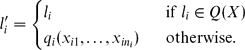
We construct the mbotM′ = (Q′, Σ, Δ, F′, R′) such that

• • Q′ = Q ∪ {q ₁,. .nbsp;.,q _k},

• • F′(q) = F(q) for every q ∈Q ₁ and F′(q _i) = 0 for every i ∈ [k] with n _i = 1,

• • for every (l′, r′) ∈ supp(R)

  

• • R′(l _i, l′_i) = 1 for every i ∈ [k] such that l _i ∉ Q(X), and

• • R′(σ(l′₁,. . .,l′_k), r) = R(l, r).

It is straightforward to prove that M′ and M are equivalent. This can easily be proved using the derivation semantics because every derivation that uses the rule (l, r) of M can be simulated by several rules of M′. Moreover, since the states q ₁,. . .,q _k do not have any other rules any derivation in M′ will simulate the effect of the rule (l, r). Let m = max{|l|_Σ | (l, r) ∈ supp(R)}. Clearly, M′ will have one less rule with m input symbols than M. Hence, repeated application of the above construction eventually yields an equivalent mbotM″ = (Q″, Σ, Δ, F″, R″) such that |l|_Σ ≤ 1 for every (l, r) ∈ supp(R″). Moreover, the process clearly terminates in time (|M|). □

In Figures 1 and 2 we show rules and their corresponding rules in binarized form (i.e., with binarized trees in the rules). It is known (Aho and Ullman Reference Aho and Ullman1972) that, in general, stsg (or scfg or extended top-down tree transducers) cannot be binarized. In Figure 3 we illustrate the binarization construction in the proof of Theorem 6 on the rule of Figure 2. How the decomposed rules combine into the original rule is demonstrated in Figure 4, which also shows two example derivation steps. In the next section, we show one benefit of the binarization on the Bar-Hillel construction.

Corollary 7 (of Theorem 6)

For every stsgM an equivalent, binarized mbot can be constructed in (|M|).

Finally, let us shortly discuss why we call ‘binarized’ also ‘input binarized’. In a binarized mbot each rule concerns at most two input subtrees. Note that the variables of X in rules represent output trees. Consequently, we can call the mbotM = (Q, Σ, Δ, F, R) output binarized if |r|_X ≤ 2 for all (l, r) ∈ supp(R). We already mentioned that stsg cannot be binarized and these problems translate into output binarization. More specifically, binarizable stsg (Zhang et al. Reference Zhang, Huang, Gildea, Knight, Moore, Bilmes, Chu-Carroll and Sanderson2006; Wang et al. Reference Wang, Knight, Marcu and Eisner2007) can be transformed into output-binarized mbot, but in general, mbot cannot be output-binarized.

5 Input and output restriction

A standard operation for tree transformations (and tree languages alike) is regular restriction. For transformations this operation can be applied to the input or output side. These constructions are used in parsing, integration of a language model, and the computation of certain metrics [see Nederhof and Satta (Reference Nederhof and Satta2003), Nederhof and Satta (Reference Nederhof and Satta2008), or Satta (Reference Satta2010) for a detailed account]. In addition, together with domain and range constructions (see Section 6), they can be used to prove preservation of recognizability. The construction is generally known as Bar-Hillel construction [see Bar-Hillel, Perles and Shamir (Reference Bar-Hillel, Perles, Shamir and Bar-Hillel1964) for the original construction on context-free grammars] if the restricting language is presented by a wsa.

Since stsg are symmetric, only one construction is needed for them. Let us formally define the input product. Given an stsgM = (Q, Σ, Δ, I, R) and a wsaN with states P, the input product is an stsgM′ such that

for every t ∈ T _Σ and u ∈ T _Δ. The construction of M′ is called Bar-Hillel construction for M and N. The rank of an stsg rule (t, q, u) ∈ supp(R) is rk(t, q, u) = |t|_Q. The maximal rank rk(M) = max_ρ∈supp(R)rk(ρ) of a rule of M enters as an exponent into the time complexity (|M|⋅|P|^2rk(M)+5) of the Bar-Hillel construction (Maletti and Satta Reference Maletti, Satta, Drewes and Kuhlmann2010). Since binarization is not possible in general, the maximal rank rk(M) cannot be limited to 2. In contrast, binarization is possible for mbot with only linear overhead, so we investigate whether we can exploit this advantage in a Bar-Hillel construction for mbot.

We start with a classical product construction for the input side. Given an mbotM = (Q, Σ, Δ, F, R) in one-symbol normal form such that the symbols in Σ ∪ Δ have rank at most 2 and a tsgN = (P, Σ, Σ, I, R′) that is also a scfg (see Proposition 1), we want to construct an mbotM′ such that M′(t, u) = M(t, u)⋅N(t) for every t ∈ T _Σ and u ∈ T _Δ. In other words, each input tree should be rescored according to N; in the unweighted case this yields that the translation of M is filtered to the set of input trees accepted by N.

We occasionally use the angled parentheses ‘〈’ and ‘〉’ instead of the standard parentheses.

Definition 8

The input product Prod(N, M) is the mbot

such that

• • F″(〈p, q〉) = I(p)⋅F(q) for every p ∈ P and q ∈ Q ₁,

• • for every rule (l, r) ∈ supp(R) with l = q(x_{i 1},. . .,x _{i k}) and r = q′(r ₁,. . .,r _n) where q ∈ Q _k, q′ ∈ Q _n, and r ₁,. . .,r _n ∈ T _Δ(X), and for every p ∈ P, let

  

• • for every (l, r) ∈ supp(R) with

  
  and r = q(x _{j 1},. . .,x _{j n}) where σ ∈ Σ_k, q, q ₁,. . .,q _k ∈ Q, and for every p, p ₁,. . .,p _k ∈ P, let

  • — ,

  • — , and

  • — .

The first type of rule constructed in the second item does not involve an input symbol. Thus, the nonterminal p of N is just forwarded to the new state in the right-hand side. Since no step with respect to the tsgN is made, the weight is taken from the rule of M. The second type of rule constructed in the third item uses a rule of R with the input symbol Σ and a rule of R′ that also contains Σ. Both rules are executed in parallel in the resulting rule and its weight is the product of the weights of the original rules. Overall, this is a classical product construction, which is similar to other product constructions such as Borchardt (Reference Borchardt2004).

Theorem 9

For every stsgM = (Q, Σ, Δ, F, R) in one-symbol normal form and tsgN = (P, Σ, Σ, I, R′) that is also an scfg, we have

for every t ∈ T _Σ and u ∈ T _Δ.

Proof

Let M″ = Prod(N, M) = (P × Q, Σ, Δ, F″, R″). We first prove that

for every p ∈ P, q ∈ Q _n, t ∈ T _Σ, and u ₁,. . .,u _n ∈ T _Δ. Let ξ = 〈p, q〉(u ₁,. . .,u _n) and t = σ(t ₁,. . .,t _k) for some σ ∈ Σ_k and t ₁,. . .,t _k ∈ T _Σ.

Now we can complete the proof as follows. For every t ∈ T _Σ and u ∈ T _Δ

□

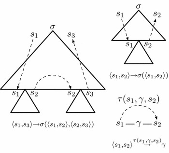
Finally, let us discuss the time complexity. The mbotProd(N, M) can be obtained in time (|M|⋅|N|). Furthermore, it is known [see, for example, Maletti and Satta (Reference Maletti, Satta, de la Clergerie, Bunt and Danlos2009)] that for every wsaN with states P, we can construct a tsgN′ that is also a scfg, which has size (|Σ|⋅|P|³), such that N′(t) = N(yd(t)) for every t ∈ T _Σ. The main idea of this well-known construction is illustrated in Figure 5.

Fig. 5.

Constructing a tsg from a wsa.

Corollary 10 (of Theorem 9)

For every mbotM = (Q, Σ, Δ, F, R) and every wsaN = (P, Γ, I, ν, G), an mbotM′ can be constructed in time (|M|⋅|P|³) such that M′(t, u) = M(t, u)⋅N(yd(t)) for every t ∈ T _Σ and u ∈ T _Δ.

Thus, our Bar-Hillel construction has the well-known (parsing) complexity (|M|⋅|P|³). Compared to the time complexity (|M|⋅[|P|^2rk(M)+5) of the Bar-Hillel construction for an stsgM, a huge efficiency gain is achieved by binarization (and one-symbol normal form). In fact, if the original stsgM is binarizable (i.e., rk(M) = 2), then the Bar-Hillel construction can still run in time (|M|⋅|P|⁶⁺³), which is due to the fact that several symbols can occur in each rule. This can be explained on the left illustration of Figure 5. If several symbols are present in the tree represented by a triangle in the illustration, then the arrows need no longer indicate identity. Consequently, all indicated state positions could hold different states, which yields the factor (|P|⁶). Since we also have to run the wsaN on several symbols, we obtain a processing factor (|P|³). The latter factor is a pure processing factor, so the size of the output stsg would be bound by (|M|⋅|P|⁶). Only if a normal form analogous to one-symbol normal form can be achieved for M, then the complexity reduces to (|M|⋅|P|³). Consequently, the stsgM should be transformed into an equivalent mbot in one-symbol normal form, which can be achieved in linear time (see Corollary 7, and the Bar-Hillel construction should be performed on this mbot.

Since mbot are not symmetric, a special construction is needed for the output side. We will see that we cannot obtain a similar efficiency improvement in this case. To simplify the presentation, we assume without loss of generality that the variables occur in order in l (i.e., l is k-normed) for every rule (l, r) ∈ supp(R).

Definition 11

The output product Prod(M, N) is the mbot

where

• • F″(q〈p〉) = I(p)⋅F(q) for every p ∈ P and q ∈ Q ₁,

• • for every rule (l, r) ∈ supp(R) with l = q(x _{j 1},.–.–.,x _{j k}) and

  
  where q ∈ Q _k, q′ ∈ Q _n and δ ∈ Δ_m−j, and for every p, p ₁,. . .p _k ∈ P, let

  • — ,

  • — ,

  • — , and

  • — ,

• • for all (l, r) ∈ supp(R) with l = and where , and , let

  • — ,

  • — ,

  • — , and

  • — .

Since the first type of rule constructed in the second item involves an output symbol, we perform steps with respect to M and N. The second type of rule does not contain an output symbol, and thus, the nonterminals of N are just forwarded to the right-hand side.

Theorem 12

For every mbotM = (Q, Σ, Δ, F, R) in one-symbol normal form and tsgN = (P, Δ, Δ, I, R′) that is also an scfg, we have

for every t ∈ T_ _Σ and u ∈ T _Δ.

Proof

The proof is similar to the proof of Theorem 9. □

The Bar-Hillel construction for the output side of an mbotM with a wsaN with states P can be obtained in time (|M|⋅|P|^2rk(M)+2) where rk(M) is the maximal number of variables of X in a rule of M. Compared to the time complexity (|M|⋅|P|^2rk(M)+5) of the Bar-Hillel construction for an stsgM, the efficiency gain is minimal and only due to the fact that at most one output symbol needs to be processed in the Bar-Hillel construction for mbot (because the mbot can be assumed to be in one-symbol normal form). A similar normal form cannot, in general, be obtained for stsg, and thus, an additional evaluation effort (|P|³) occurs, which represents the time complexity of running the wsaN on the output symbols present in a rule. It was already mentioned that if the stsgM is binarizable, then we can obtain an equivalent output-binarized mbot. In this case, the problem is symmetric and the results for the input product apply also for the output product.

6 Forward and backward application

Finally, we want to apply a weighted tree transformation not just to a single input or output tree, but rather to a set of (potentially weighted) input or output trees. Let M be an mbot or an stsg. Forward application aims to compute a tsg of output trees under M given a tsg of input trees. Conversely, backward application aims to compute a tsg of input trees given a tsg of output trees. Formally, let N = (P, Σ, Σ, I, R′) and N′ = (P′, Δ, Δ, I′, R″) be tsg. Then the forward application M 〈N〉) and the backward application M ⁻¹ 〈N′〉 are

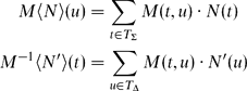
for every t ∈ T _Σ and u ∈ T _Δ. Note that the sums in the above equations might be infinite. We will later address this issue by additional restrictions, which will ensure that the sums are finite.

In general, forward and backward application can be reduced to range and domain, respectively, with the help of the product constructions of the previous section. Formally, the range ran _M and the domain dom _M of the transformation computed by M are

for every t ∈ T _Σ and u ∈ T _Δ. Again, those sums might be infinite. Let M be an mbot. The relation between the two notions is

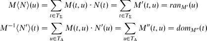
for every t ∈ T _Σ and u ∈ T _Δ where M′ = Prod(N, M) and M″ = Prod(M, N′). The same relation also holds for an stsgM.

Let us first discuss stsg. Let M = (Q, Σ, Δ, I, R) be an stsg. It is input ϵ-free (respectively, output ϵ-free) if t ∉ Q (respectively, u ∉ Q) for every (t, q, u) ∈ supp(R). It is known (Fülöp, Maletti and Vogler Reference Fülöp, Maletti, Vogler, Drewes and Kuhlmann2010) that the forward application M〈N〉 (respectively, the backward application M ⁻¹〈N′〉) can be represented by a tsg if M is output ϵ-free (respectively, input ϵ-free). In other words, stsg preserve recognizability under forward and backward application in all reasonable cases.

Unfortunately, the range of an mbot is not necessarily representable by a tsg, which is not due to well-definedness problems (infinite sums) but rather the finite-copying property (Engelfriet et al. Reference Engelfriet, Rozenberg and Slutzki1980) of mbot. Because of this copying property the range might not be recognizable. Consequently, forward application suffers from the same problem, which yields that mbot do not preserve recognizability under forward application. In analogy to the definition for stsg, let the mbotM = (Q, Σ, Δ, F, R) be input ϵ-free} if l ∉ Q(X) for every (l, r) ∈ supp(R). For such mbot we will now discuss the domain (and backward application).

Definition 13

Let M = (Q, Σ, Δ, F, R) be an input ϵ-free mbot such that Q _i ∩ Q _j = ∅ for all i ≠ j. In other words, we assume without loss of generality that each state has a unique rank. We construct the tsgN = (Q, Σ, Σ, I, R′) such that

• • I(q) = F(q) for every q ∈ Q ₁ and I(q) = 0 for all q ∈ Q ∖ Q ₁,

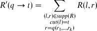
• • for every t ∈ T _Σ(Q)

  
  where cut(l) ∈ T _Σ(Q) is tree obtained from l ∈ T _Σ(Q(X)) by deleting the nodes labeled by an element of X.

Theorem 14

Let M be an input ϵ-free mbot and N be the tsg as in Definition 13. Then dom _M = N.

Proof

We need to prove that for every q ∈ Q _k and t ∈ T _Σ.

Then

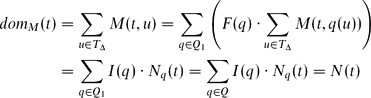
for every t ∈ T _Σ, which proves the statement. □

Consequently, every input ϵ-free mbot preserves recognizability under backward application, which is essentially the same statement as for stsg. However, the situation is entirely different for forward application. stsg preserve recognizability under forward application, but mbot do not necessarily.