Implications
The e-Cow model predicts the performance of dairy cows of different genetic merit, grazing either ryegrass or lucerne-based pastures, with or without supplementary feeding, thus being useful for conditions in different countries. The model is sensitive to genotype × environment interactions.
The e-Cow model is useful for applied research, teaching and extension purposes, allowing a quick and practical understanding of the effects of feeding level, that is, pasture and supplements offered, and cow's genetic merit on herbage dry matter intake, milk yield and changes in body condition score and live weight. The e-Cow model is a tool to aid decision making around management strategies.
Introduction
When simulating the performance of grazing dairy cows, three of the most important challenges faced are: (i) the prediction of herbage dry matter (DM) intake (Delagarde and O'Donovan, Reference Delagarde and O'Donovan2005), (ii) the combination of nutritional and genetic mechanisms controlling energy partitioning within the cow (Friggens et al., Reference Friggens, Ingvartsen and Emmans2004) and (iii) the inclusion of genetic differences between cows in the prediction of both herbage DM intake and energy partitioning (Bryant et al., Reference Bryant, Lopez-Villalobos, Holmes and Pryce2005). Few mathematical simulation models address these challenges simultaneously.
The prediction of herbage DM intake at grazing is complex because of the characteristics of the swards and animals and the biological processes involved in food selection, ingestion and digestion. This study proposes an approach to predict intake based on an easy-to-obtain set of inputs, combining theoretical and empirical equations that account for physical (rumen fill), metabolic (energy demand) and ingestive restrictions.
The prediction of the energy allocated to either milk outputs or body lipid reserves, that is, energy partitioning, is a long-standing problem that has not been solved. Traditionally, nutritional models approach nutrient partitioning within the cow as a homeostatic function of changing nutritional environment, solving divergences between nutrient intakes and milk outputs by adjusting body fat reserves up or down (Friggens and Newbold, Reference Friggens and Newbold2007). However, coordinated changes in metabolism of body tissues, necessary to support a physiological state, were also recognised in dairy cows. The mechanisms explaining these changes, which occur as a function of (physiological) time rather than as a function of changing nutritional environment, were defined as homeorhetic mechanisms (Bauman and Currie, Reference Bauman and Currie1980). Thus, an aspect of nutrient partitioning is genetically driven and, therefore, nutrient partitioning will change throughout lactation according to the genotype of the cow and cannot be predicted only from feed intake and milk outputs (Friggens and Newbold, Reference Friggens and Newbold2007).
Few nutritional models incorporate genetic differences between cows (Bryant et al., Reference Bryant, Lopez-Villalobos, Holmes and Pryce2005), and even less are adapted to grazing dairy cows. Bryant et al. (Reference Bryant, Lopez-Villalobos, Holmes, Pryce, Rossi and Macdonald2008) developed a model that predicts the performance of dairy cows at grazing and accounts for genetic differences between cows. This model was validated for cows in early lactation, with acceptable accuracy of prediction for milk yield, but with low accuracy of prediction for herbage DM intake and live weight (LW) change.
The objectives of this study are: (i) to develop an animal model able to predict herbage DM intake at grazing, including nutritional and genetic mechanisms controlling energy partitioning within the cow and accounting for genetic differences between cows, (ii) to validate the animal model with a dataset from cows of different genetic merit grazing a forage diet, with and without concentrate supplementation and (iii) to simulate animal performance in different feeding scenarios to explore the sensitivity of the model to genotype × environment, that is, feeding environment interactions.
Major efforts have been devoted to the development and validation of simulation models that predict DM intake, milk yield or body lipid changes separately for dairy cows. Therefore, it is important to integrate these models to represent more accurately the priorities and performance of dairy cattle.
Material and methods
Model overview
This model, named e-Cow, integrates three previously published models: (i) a model that predicts herbage DM intake for grazing dairy cows (Baudracco et al., Reference Baudracco, Lopez-Villalobos, Holmes and Macdonald2010a), hereafter named the INTAKE model; (ii) a mammary gland model (Vetharaniam et al., Reference Vetharaniam, Davis, Upsdell, Kolver and Pleasants2003) that predicts potential milk yield, hereafter named the MILK model; and (iii) a body lipid model (Friggens et al., Reference Friggens, Ingvartsen and Emmans2004) that predicts genetically driven LW and body condition score (BCS), hereafter named the LIPID model. Therefore, e-Cow predicts, on a daily basis, herbage DM intake, milk yield, BCS, LW and changes in BCS and LW for grazing dairy cows.
The rationale of the e-Cow model is that the total metabolisable energy (ME) consumed (MEItkTotal, ME consumed from herbage plus supplements) calculated using the INTAKE model must be equal to the sum of all ME requirements (equation 1), namely: ME for maintenance (MEm) and pregnancy (MEp; Freer et al., Reference Freer, Dove and Nolan2007); ME for growth in the case of young animals (MEgr; SCA, 1990); ME required for milk synthesis (ME Potential Milk Yield; see MILK model description below); and ME mobilised or synthesised from/to body lipid reserves (ME from/to BCS change; see LIPID model description below). Both ME Potential Milk Yield and ME from/to BCS change represent the milk synthesis and BCS change genetically driven, which are later adjusted by the nutritional status of the cow as explained below:

The difference between ME intake and all the ME requirements is named ME Balance, and can be obtained by rearranging equation (1), as follows:

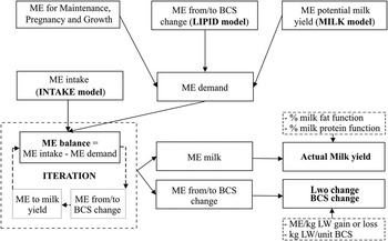
Equations (1 and 2) integrate the INTAKE model, which provides the amount of energy consumed (pasture plus supplements), with the MILK and LIPID models, which provide the potential milk yield and BCS change, respectively, if no nutritional limitations occur. However, ME Balance will differ from zero when nutritional limitations occur, as it is usually the case in grazing dairy systems. In order to integrate the three models, ME Balance must be equal to zero. If ME Balance is less than zero, then an iterative procedure is used to reduce ME Potential Milk Yield and increase BCS loss (or decrease BCS gain) each by 1% of itself, until ME Balance is set to zero. A schematic overview of the model is depicted in Figure 1. The e-Cow model is written in Visual Basic programming language within Microsoft Excel®.
Schematic representation of the e-Cow model, showing the integration of INTAKE, MILK and LIPID models to predict metabolisable energy (ME) partitioning within the cow. LW = live weight; LWo change = LW change associated with body condition score (BCS) change.

The extent to which ME from/to BCS change and ME Potential Milk Yield are adjusted in the iteration depends on the stage of lactation, because they are adjusted each time within the iteration as a proportion (1%) of their initial predictions. The initial predictions come from the LIPID and MILK models (explained below), and depend on the stage of lactation.
Prediction of DM intake – INTAKE model
Limits to herbage DM intake
The INTAKE model initially predicts herbage DM intake of grazing dairy cows offered only pasture, and then the total DM and total ME intakes if supplements are used. The model sets an upper limit to potential herbage DM intake at grazing (PotDMI) for cows offered only pasture, which is the minimum out of three limits: (i) physical limitation related to rumen fill (PotDMIr), (ii) metabolic limitation related to energy demand (PotDMIe) and (iii) a ‘grazing limit’ related to ingestive constraints (PotDMIg).
The principles of the physical limitation model developed by Mertens (Reference Mertens1987) are used to calculate the PotDMIr. Merten's model states that, when the fill effect of the diet is high, the daily potential intake (PotDMIr) can be expressed as a constant rumen capacity divided by the fill effect of the diet. In this model, it was assumed that the animal has a potential NDF rumen capacity (0.0165 × LW) and that the feeds have a given capacity to occupy space determined by its NDF content. Thus, the PotDMIr is calculated as the ratio between rumen capacity and the fill effect of the diet (proportion of NDF in the diet) times a coefficient accounting for the effect of stage of lactation on rumen capacity. The term 0.0165 times LW is supported by data from Vazquez and Smith (Reference Vazquez and Smith2000), which show that, at high herbage allowance (HA), the average daily intake of NDF was 1.65% of LW.
The metabolic limit to intake (PotDMIe) is calculated as follows:

where MEReq (MJ ME/cow per day) is the right-hand side of equation (1) and PastME is the ME content of herbage (MJ ME/kg DM).
The grazing limit (PotDMIg) is set at 37.5 g herbage DM intake/kg LW times a coefficient accounting for the effect of stage of lactation on maximal ruminal capacity. This value of 37.5 g DM intake/kg LW is based on the maximum intakes measured for high-yielding Holstein–Friesian (HF) cows grazing with no pasture quality or quantity restrictions (Kolver and Muller, Reference Kolver and Muller1998). However, this limit can be modified through the input screen described below, under the title ‘input and outputs screens of the e-Cow model’ to represent the situation of a particular breed or strain. Further details of the three limits to potential DM intake can be found in Baudracco et al. (Reference Baudracco, Lopez-Villalobos, Holmes and Macdonald2010a).
Herbage DM intake
Then, the minimum of these three PotDMI limits and the HA (kg DM/cow per day) are used to predict herbage DM intake for cows offered only pasture using empirical algorithms (equations 4 to 6). These algorithms are derived from unsupplemented treatments in experiments with cows grazing ryegrass-based pastures or lucerne-based pastures. From those treatments, the ratio HA : PotDMI was calculated and regressed against the measured harvesting efficiency (HE), that is, efficiency of grazing. The ratio HA : PotDMI is a measure of the pasture offered relative to the cow's demand for pasture at grazing. The empirical equations obtained from those regressions are used to predict HE and the actual herbage DM intake of cows offered only pasture (equations 4, 5 and 6). For ryegrass-based pastures, equations were derived from two types of experiments: those that measured allowance at ground level and those that measured allowance at a cutting height of approximately 4 cm above the ground level. The equation obtained for ryegrass-based pasture with HA expressed at the ground level is (Baudracco et al., Reference Baudracco, Lopez-Villalobos, Holmes and Macdonald2010a)

while the equation obtained for ryegrass-based pasture with HA expressed at a cutting height of 4 cm above the ground level, derived from experiments detailed in Table 1 of Baudracco et al. (Reference Baudracco, Lopez-Villalobos, Holmes and Macdonald2010b) is

and for lucerne-based pastures, with HA expressed at 4 cm above ground level, the equation is (Baudracco et al., Reference Baudracco, Lopez-Villalobos, Holmes, Brookes, Kemp, Comeron, Romero, Horan, Dillon and Berry2006)

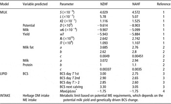
Default parameters used in the e-Cow model to predict potential milk yield (MILK model), body lipid change genetically driven (LIPID model) and herbage intake (INTAKE model) for NZHF and NAHF cows

NZ = New Zealand; NA = North America; HF = Holstein–Friesian; BCS = body condition score; ME = metabolisable energy; TMR = total mixed ration.
1Vetharaniam et al. (Reference Vetharaniam, Davis, Upsdell, Kolver and Pleasants2003), with constant S re-parameterised for mature cows offered TMR diets from Kolver et al. (Reference Kolver, Roche, Veth, Thorne and Napper2002).
2Wilmink function parameters reported by Roche et al. (Reference Roche, Berry and Kolver2006).
3Assumtions based on Friggens et al. (Reference Friggens, Ingvartsen and Emmans2004) and results from Horan et al. (Reference Horan, Dillon, Faverdin, Delaby, Buckley and Rath2005) and McCarthy et al. (Reference McCarthy, Berry, Dillon, Rath and Horan2007).
4Values proposed by Friggens et al. (Reference Friggens, Ingvartsen and Emmans2004).
*MaxLipLoss is a maximal rate of lipid loss (kg/day; Friggens et al., Reference Friggens, Ingvartsen and Emmans2004).
Then, herbage DM intake (of cows offered only pasture) is obtained by multiplying HE times HA.
Herbage DM intake of supplemented cows
When supplements are offered, the herbage DM intake of cows offered supplements (HerbDMIs) is calculated as

where HerbDMIo is the herbage DM intake of cows offered only pasture. Substitution rate (SR) expresses the decrease in kg DM intake of herbage per kg DM intake of supplement (SuppDMI), and is calculated as follows (Stockdale, Reference Stockdale2000):

where HDMI is herbage DMI before supplementation, expressed as kg DM/100 kg LW. Equation (8) can be modified by the user to accommodate to particular situations with expected lower or higher SR. Figure 4a shows a button (SR equation) to edit the parameters of the SR equation.
Prediction of milk yield – MILK model
The ME Potential milk yield is calculated using a mathematical mammary gland model (Vetharaniam et al., Reference Vetharaniam, Davis, Upsdell, Kolver and Pleasants2003), which is based on the interaction of two pools of alveoli (i.e. groups of secretory cells): one active pool and one non-active pool. The active alveoli are produced by progenitor (undifferentiated) cells. Throughout lactation, active alveoli can proceed to a state of quiescence (non-secretory cells) and these quiescent alveoli then become either reactivated to active alveoli or proceed to senescence. In this model, the amount of ME required to achieve the potential milk yield of a cow is calculated using the following equation:

where S is the maximum milk secretion rate of active alveoli, t is the time after calving (days), E is the energy status at day t (set to 1 to calculate ME Potential milk yield, no nutritional limitations), L is a genetic parameter that governs the response of milk yield to nutrition (constant for each genotype, see Table 1), d, l6 and l7 define the number of active alveoli, K2 is a constant defining the rate of decay of production of active alveoli with time and w6 and w7 are parameters related to the rates at which active alveoli proceed to quiescence, the rate at which quiescent alveoli are reactivated to become active alveoli and the rate at which quiescent alveoli proceed to senescence (Table 1). Detailed explanation of the latter parameters and the alveolar dynamic can be found in Vetharaniam et al. (Reference Vetharaniam, Davis, Upsdell, Kolver and Pleasants2003). As shown in equation (10) (Freer et al., Reference Freer, Dove and Nolan2007), Kl is a coefficient accounting for the efficiency of utilisation of ME for milk synthesis:

where MEdiet is the weighted average energy content of feeds consumed (MJ ME/kg DM).
In the e-Cow model, ME Potential milk yield is estimated using the parameters reported by Vetharaniam et al. (Reference Vetharaniam, Davis, Upsdell, Kolver and Pleasants2003) for first lactation cows of both New Zealand (NZ) HF and North American (NA) HF strains offered total mixed ration (TMR) diets (no nutritional limitations). The constant S was re-parameterised for mature cows offered TMR diets, based on the results reported by Kolver et al. (Reference Kolver, Roche, Veth, Thorne and Napper2002). The adjusted potential yields of mature cows (305-day lactation) after re-parameterisation are 11 247 and 8011 kg milk per cow and 836 and 679 kg milksolids per cow for NAHF and NZHF strains, respectively. These are default values of potential milk yield internally stored in the model. However, they can be modified if a different potential milk yield is set as input, or if an immature cow (less than four lactations) is simulated.
When the input ‘potential milk yield’ differs from the internally stored values, that is, 11 247 and 8011 kg milk/cow for NAHF and NZHF strains, an iterative procedure is used to determine the value of the parameter S that produces a lactation curve with the new potential milk yield (kg milk for 305 days). An age-production factor is used to adjust the potential milk yield for young cows. Multiplicative age adjustment factors for milk yields are 0.75, 0.87, 0.95, 1.0, 0.97 and 0.92 for lactations 1, 2, 3, 4 to 7, 8 and 9, respectively (Lopez-Villalobos et al., Reference Lopez-Villalobos, Garrick, Holmes, Blair and Spelman2000). These factors can be modified by clicking on the button ‘milk model parameters’ of Figure 4a.
In the iterative procedure shown in Figure 1, ME Potential Milk Yield is converted into MEmilk, the latter being the ME available for Actual Milk Yield. Then, MEmilk is divided by MEl to calculate Actual Milk Yield (kg/cow per day). The MEl is the ME required to synthesise 1 kg of milk and is calculated as the net energy content of milk (Freer et al., Reference Freer, Dove and Nolan2007) divided by Kl as follows:

Percentages of milk fat (PercMilkFat) and percentage of milk protein (PercMilkProt) are required to calculate the energy content of milk. Lactation curves for milk fat and milk protein contents are modelled using the Wilmink (Reference Wilmink1987) function:

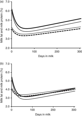
where yt represents the percentages of milk fat or milk protein at day t of lactation and e is the base of the natural logarithm (2.718281828), while a, b and c are parameters that define the shape of the curve. The values for parameters a, b and c were obtained from Roche et al. (Reference Roche, Berry and Kolver2006), for both NZHF and NAHF cows. Parameters a, b and c are adjusted in the e-Cow model according to the amount of concentrate in the diet, based on the parameters reported by Roche et al. (Reference Roche, Berry and Kolver2006) for cows offered different amounts of concentrates. Examples of predicted concentrations of milk fat and milk protein by the e-Cow model, for cows consuming either 0 or 6 kg DM/cow per day concentrate, are given in Figure 2.
Example of predicted concentration of milk fat and milk protein throughout lactation for (a) New Zealand Holstein–Friesian cows and (b) North American Holstein–Friesian cows. Milk fat content for cows consuming either 0 ( ) or 6 (—) kg DM/cow per day concentrate. Milk protein content for cows consuming either 0 (- - -) or 6 (. . . . .) kg DM/cow per day concentrate.

Prediction of BCS and LW – LIPID model
The model proposed by Friggens et al. (Reference Friggens, Ingvartsen and Emmans2004) is used to predict the genetically driven pattern of body lipid change throughout pregnancy and lactation. This LIPID model is based on evolutionary arguments suggesting that at any given time in pregnancy and lactation, there is an optimal level of body fatness that the animal is genetically driven to accomplish.
The LIPID model proposes that mobilisation and gain of body reserves are genetically driven to achieve two target levels of body fatness: one at, or around, conception and another at the next calving. Thus, cows in good body condition at calving will allocate large amounts of their energy reserves and energy intake towards milk yield, reducing their BCS to achieve the target level of fatness at conception. In contrast, cows at a low BCS at calving will adjust mechanisms of nutrient partitioning and lipogenesis to increase BCS, to attain the target genetic level of fatness at conception. After conception, the model predicts that cows will gradually increase body condition in order to meet the target BCS at next calving. As explained below, this target BCS at next calving depends on the genetic merit of the cow.
Assumptions of the LIPID model
The following assumptions are made for a cow of a given size:
1. The cow is driven to have a target amount of body lipid mass (L, expressed in kg) at a particular time in lactation (T, expressed as days from calving). The T value used is 112 days in milk (DIM).
2. The rate of change of body lipid, dL/dt (kg/day), changes linearly with time between calving and day T. The expression ‘dt’ refers to 1 day.
3. If pregnant, the cow is driven to have a specific amount of lipid at the next calving, called Lnext (kg).
4. The rate of change of body lipid dL/dt (kg/day), changes linearly with time between conception and the next calving (Lnext, kg).
5. At times greater than T, and if the cow is not pregnant then dL/dt is assumed to be 0, that is, the cow has no drive to increase body lipid mass.
6. There is a maximal rate of lipid loss, called MaxLipLoss (kg/day). This is a negative value of dL/dt.
There are minor adjustments for this model, related to the value of T, that can be found in Friggens et al. (Reference Friggens, Ingvartsen and Emmans2004).
Estimation of body lipid mass from LW and BCS
Body lipid mass (L) at calving is calculated as the product of empty body weight (BW) and the proportion of lipid in the empty body (equation (13); Friggens et al., Reference Friggens, Ingvartsen and Emmans2004). To convert BCS (measured on a 0 to 5 scale) into body lipid proportion, the following equation is used:

The empty BW is calculated as the difference between LW standardised at BCS 3 and gut fill, the latter assumed as 15% of LW at BCS 3. The LIPID model assumes that the LW associated with a unit change BCS is 12.9% of LW at BCS 5 (BCS standard). The LW at the BCS standard is calculated as

The inputs required by the LIPID model are BCS and LW at calving and the date of conception (days after calving). The default parameters used in the model are listed in Table 1.
The LW0 change (LW change due to changes in BCS) and BCS change are calculated using the ME associated with BCS change (ME from/to BCS Change) resulting from the iteration (Figure 1), the ME required to synthesise/mobilise 1 kg LW and the kg of LW per unit of BCS. The energetic cost associated with LW0 change (MJ ME/kg LW gain or LW loss) is calculated based on the equations proposed by AFRC (1990).
It is important to notice that the LIPID model predicts only the genetically driven changes in BCS and LW0, and assumes no nutritional constraints. However, when integrated into the e-Cow model, LW0 and BCS changes depend on the nutritional status of the cow, given that ME from/to BCS change is recalculated in the iteration (see Figure 1), and adjusted according to the ME Balance of the cow. For example, after conception, the LIPID model predicts that cows will gradually increase BCS to meet the target BCS at next calving; however, the iteration introduces a nutritional component and therefore, the e-Cow model will predict that the cow loses BCS after conception if the energy intake is very low.
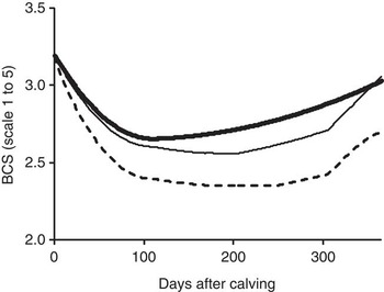
Figure 3 shows an example of the original BCS curve predicted with the LIPID model and two BCS curves for either low or high nutritional levels when the LIPID model is integrated into the e-Cow model.
Example of BCS curves predicted with ( ) the LIPID model (Friggens et al., Reference Friggens, Ingvartsen and Emmans2004) and with the e-Cow model for North American Holstein–Friesian cows offered either pasture plus 6 kg DM concentrates (—) or only-pasture diet (
 ). Example for cows in second lactation, offered herbage allowance of 50 kg/cow per day, with 11.0 MJ/kg DM herbage.

Energy requirements for maintenance, pregnancy and growth
The e-Cow model assumes that the requirements for maintenance, growth and pregnancy are satisfied before all other requirements.
Maintenance
The ME required for maintenance (MEm) is calculated as follows (Freer et al., Reference Freer, Dove and Nolan2007):

where A is the age in years, Km is the net efficiency of use of ME for maintenance calculated as 0.02MEdiet + 0.5, MEdiet is the weighted average ME concentration of the feed available (MJ/kg DM), MEmilk is the amount of dietary ME being used directly for milk production and Egraze is the additional energy expenditure of a grazing animal compared with a similar housed animal (Freer et al., Reference Freer, Dove and Nolan2007).
Pregnancy
Gestation length is assumed to be 284 days. Requirements of ME to maintain pregnancy (MEp) are calculated using the standard equations proposed by SCA (1990).


LW gain due to growth
The LW gain due to growth (LWgr) of young animals must be included in the final calculation of LW change. The e-Cow model assumes that cows in their first, second and third lactation will grow to ensure target LW at maturity. The LW gain due to growth is calculated on the basis of the difference between target weights at two consecutive lactations. It is assumed that target weights (Target LW) post calving are 85%, 92% and 96% of mature weight for cows in first, second and third lactation, respectively (Fox et al., Reference Fox, van Amburgh and Tylutki1999). These values are set as default in the model but can be modified by clicking on the button ‘LIPID model parameters’ of Figure 4a. The daily growth is assumed to be linear between lactations, and is calculated as follows:

where Target LWnext and Target LW are the postcalving LW at the next and the present lactation, respectively.
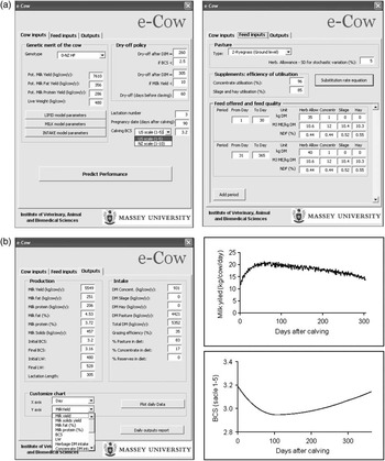
Visual Basic interface screens of e-Cow inputs (a) and outputs (b). The charts appear when clicking on ‘plot daily data’ button in the ‘customised chart’ section of the output screen (b).

LW gain due to pregnancy
The LW change predicted with the LIPID model represents only the LW associated with body lipid reserves (LW0). For pregnant animals, LWgain due to growth of the gravid uterus (LWp) should be added to the predicted daily LW0 change. It can be calculated as follows (Fox et al., Reference Fox, van Amburgh and Tylutki1999):

where CBW is the calf birth weight in kg, t is the time pregnant (days) and e is the base of the natural logarithm (2.718281828).
Inputs and outputs screens of the e-Cow model
Figure 4 shows the Visual Basic interface screens developed for the e-Cow model. In the ‘cow inputs’ tab of Figure 4a, by defining the genotype of the cow and the lactation number, the default values from Table 1 will be used to estimate the potential yields of milk, fat and protein. The e-Cow model calculates the potential milk fat and milk protein yields (kg/cow in 305-day lactation) by multiplying the daily percentages of milk fat and milk protein by the daily potential milk yield, and then summing the milk fat and milk protein yields for the whole lactation. These calculated potentials can be modified by using a different potential fat and protein yields as input (kg/cow in 305-day; Figure 4a, ‘cow inputs’ tab, ‘genetic merit of the cow’). If the potential yields are modified, then, an iterative procedure is used to find a new value for the parameter a of the Wilmink function for the curves of milk fat and milk protein percentages, to obtain the new potential yields of milk fat and milk protein (305 days in milk) set as inputs. Furthermore, the parameters shown in Table 1 can be manually changed by selecting the buttons LIPID model, MILK model and INTAKE model parameters in the ‘cow inputs’ tab (Figure 4a).
Lactation can be stopped at any stage, that is, before or after 305 days, by setting a dry-off policy (Figure 4a, Dry-off Policy), defining a threshold value for either BCS or milk yield or the number of days before next calving date. When any of these threshold values is achieved, the lactation will be finished. The BCS at calving can be set using the US or the NZ system, and conversions between systems are calculated according to Roche et al. (Reference Roche, Friggens, Kay, Fisher, Stafford and Berry2009).
In the ‘feed inputs’ tab (Figure 4a), by defining the type of pasture, the pertinent equations (4, 5 or 6) will be used to predict herbage DM intake at grazing. Then, in the same tab, the amounts, ME and NDF contents of pasture and supplements offered can be defined, for as many periods as desired. Daily HA can be simulated stochastically (with normal distribution), with the mean being the input value of HA per period and the s.d. being the input value set as ‘herb. allowance s.d. for stochastic variation’ expressed as a percentage of the mean HA (Figure 4a, ‘feed inputs’ tab).
The ‘outputs’ tab (Figure 4b) shows a summary of the annual production and intake variables, and allows customised charts to be plotted with the daily values for the whole lactation for the main output variables. The ‘daily output report’ button will show a table with the daily values of all the output variables.
Validation of the e-Cow model
Validation determines whether the mathematical model is an accurate representation of the real system. The parameters and equations used to build the e-Cow model were obtained from Friggens et al. (Reference Friggens, Ingvartsen and Emmans2004), Vetharaniam et al. (Reference Vetharaniam, Davis, Upsdell, Kolver and Pleasants2003), Baudracco et al. (Reference Baudracco, Lopez-Villalobos, Holmes, Brookes, Kemp, Comeron, Romero, Horan, Dillon and Berry2006, Reference Baudracco, Lopez-Villalobos, Holmes and Macdonald2010a and Reference Baudracco, Lopez-Villalobos, Holmes and Macdonald2010b), Kolver et al. (Reference Kolver, Roche, Veth, Thorne and Napper2002), Roche et al. (Reference Roche, Berry and Kolver2006), Horan et al. (Reference Horan, Dillon, Faverdin, Delaby, Buckley and Rath2005) and McCarthy et al. (Reference McCarthy, Berry, Dillon, Rath and Horan2007).
An independent dataset was obtained from a trial that evaluated three strains of HF cows grazing ryegrass-clover pasture in NZ (Macdonald et al., Reference Macdonald, Verkerk, Thorrold, Pryce, Penno, McNaughton, Burton, Lancaster, Williamson and Holmes2008). The two strains used in the validation of e-Cow were NAHF 90S (NA90; ⩾91% NA genetics) and NZHF 90S (NZ90; ⩽24% NA genetics). The dataset comprised information about 60 cows of each of these two strains, over three full lactations (1st, 2nd and 3rd parities). Data used as input in e-Cow were DIM, days pregnant, BCS at calving, LW at calving, lactation number, HA, supplements DM intake, herbage NDF, herbage ME content and supplements ME content. All data were averaged across week of lactation for each of the three parities, resulting in 135 points for validation in each of the two strains.
The concordance correlation coefficient (CCC; Lin, Reference Lin1989) and the relative prediction error (RPE; Fuentes-Pila et al., Reference Fuentes-Pila, Ibanez, Miguel and Beede2003) were used to evaluate the extent of agreement between the actual and the predicted values. The CCC is calculated as CCC = ρ × Cb, with ρ being the Pearson correlation coefficient and Cb the bias correction factor, which is calculated as

where σA, σP, μA and μP are the s.d. and mean of the actual and predicted values, respectively. The Pearson correlation coefficient reflects precision, that is, the degree to which the predicted against actual values cluster about the regression line. The bias correction factor reflects accuracy, that is, degree to which the regression line adheres to the 45° line through the origin. The scale of Landis and Koch (Reference Landis and Koch1977) has been used here to describe the degree of concordance, with 0.21 to 0.40 being ‘fair’; 0.41 to 0.60 being ‘moderate’; 0.61 to 0.80 being ‘substantial’; and 0.81 to 1.00 being ‘almost perfect’.
The RPE is defined as the positive square root of the mean square prediction error (MSPE; equation 21), expressed as a percentage of the mean of the actual values (μA; Fuentes-Pila et al., Reference Fuentes-Pila, Ibanez, Miguel and Beede2003):

where P represents the predicted values and A represents the actual observed values for either herbage DM intake, milk yield, BCS change or LW change. Fuentes-Pila et al. (Reference Fuentes-Pila, DeLorenzo, Beede, Staples and Holter1996) suggested that an RPE value lower than 10% is an indication of satisfactory prediction, whereas an RPE between 10% and 20% indicates a relatively acceptable prediction and an RPE greater than 20% indicates poor prediction.
Results
Model validation
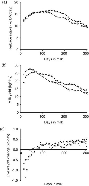
Comparison of predicted and observed data (for the whole dataset averaged per week of lactation) shows that the e-Cow model was able to simulate lactation curves of a shape similar to the observed data for herbage DM intake, milk yield and LW change (Figure 5). Predictions of herbage DM intake were very close to observed data, with a slight overestimation in mid and late lactation (Figure 5a). Milk yield was underestimated in early lactation and overestimated in mid and late lactation (Figure 5b). Predictions of LW change were generally higher than observed, but underpredicted for the first few weeks of lactation (Figure 5c).
Comparison between predicted (▴) and actual data (x) for (a) herbage dry matter intake, (b) milk yield and live weight change (c). Actual data obtained were from Macdonald et al. (Reference Macdonald, Verkerk, Thorrold, Pryce, Penno, McNaughton, Burton, Lancaster, Williamson and Holmes2008), and comprise information of three parities of Holstein–Friesian cows for both New Zealand and North American strains. The whole dataset was averaged per week of lactation.

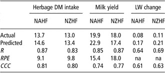
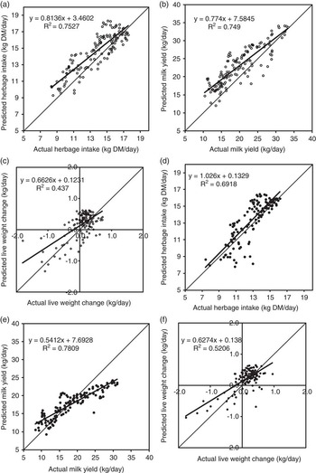
Further validation analysis for individual cow strains, and for each parity within strain, showed satisfactory accuracy of prediction, with RPE lower than 10% for herbage DM intake and between 10% and 20% for milk yield and with CCC over 0.80 for herbage DM intake, over 0.70 for milk yield and over 0.60 for LW change (Table 2 and Figure 6).
Comparison of actual (Macdonald et al., Reference Macdonald, Verkerk, Thorrold, Pryce, Penno, McNaughton, Burton, Lancaster, Williamson and Holmes2008) and predicted (e-Cow) data for daily yields of milk (kg/cow), daily herbage DM intake (kg/cow) and daily LW change (kg/cow)

DM = dry matter; LW = live weight; NAHF = North American Holstein–Friesian; NZHF = New Zealand Holstein–Friesian; R = Pearson correlation coefficient; RPE = relative prediction error; CCC = concordance correlation coefficient; na = not available.
The validation dataset includes data from NA (n = 60) and NZ (n = 60) HF cows of 1st, 2nd and 3rd parity. Data were averaged across week of lactation for each strain and parity and then analysed.
The relationship between predicted and actual values for herbage dry matter (DM) intake (kg DM/cow per day), daily milk yield (kg/cow per day) and live weight (LW) change (kg/cow per day) of North American (a, b, c) and New Zealand (d, e, f) Holstein–Friesian cows. Actual values obtained from a strain trial dataset (Macdonald et al., Reference Macdonald, Verkerk, Thorrold, Pryce, Penno, McNaughton, Burton, Lancaster, Williamson and Holmes2008) including data from 60 cows of 1st, 2nd and 3rd parity for each strain. Values averaged across week of lactation for each parity.

Predicted data were plotted against observed data for each of the two strains for herbage DM intake, milk yield and LW change (Figure 6). The average prediction of herbage DM intake was 0.9 kg DM and 0.4 kg DM higher than observed for NAHF and NZHF cows, respectively (Table 2). Differences between the average predicted and the observed milk yield (kg milk/cow per day) were +3.0 and −0.6 kg for NAHF and NZHF cows, respectively (Table 2), with a trend towards overprediction at low milk yields and underpredictions at high milk yields in both strains, which was more noticeable for NZHF cows (Figure 6e).
LW change predictions were less accurate than herbage DM intake and milk yield predictions, with overpredictions at both extremes, low and high LW changes. Differences between the average predicted and observed LW change were +0.09 and +0.10 kg/cow per day for NAHF and NZHF cows, respectively (Table 2).
The intake module included in the e-Cow model was also validated with an independent dataset from a 2-year Irish trial, with individual herbage DM intake measurements (n = 858) of three strains of lactating HF cows. The fitness of the model was satisfactory, with a RPE of 0.064 and a CCC of 0.87 (Baudracco et al., Reference Baudracco, Lopez-Villalobos, Holmes, Horan and Dillon2010c).
Model simulations
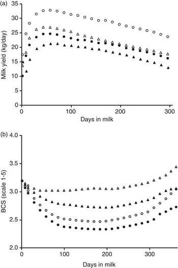
The simulated curves of milk yield and BCS throughout lactation for both NZHF and NAHF cows at two levels of feeding (0 and 6 kg DM concentrates/cow per day) can be observed in Figure 7. At the same stage of lactation, milk yield (kg milk/cow per day) was higher for NAHF than for NZHF cows and the milk response to supplementation was greater for NA than for NZ cows (Figure 7a). BCS curves differed between and within strains for different feeding levels (Figure 7b). Thus, NAHF cows could not recover the calving BCS, even when supplemented with 6 kg concentrates. In contrast, simulations for NZHF cows showed that this strain achieved a BCS at next calving of 3.1 and 3.5 when offered 0 and 6 kg concentrate/cow per day, respectively (Table 3 and Figure 7b). Furthermore, Figure 7b shows how the e-Cow model is also sensitive to the energy status of the cow, accounting not only for genetic but also for nutritional drives, as the nutrition level affected the evolution of BCS throughout lactation.
Model simulations of milk yield (a) and body condition score (BCS; b) during lactation for North American Holstein–Friesian cows consuming 0 kg (●) or 6 kg DM/cow per day concentrate (○); and for New Zealand Holstein–Friesian cows consuming 0 kg (▴) or 6 kg DM/cow per day concentrate (Δ). Example for cows in second lactation, offered herbage allowance of 50 kg/cow per day, with 11.0 MJ/kg DM herbage, and concentrates with 12.0 MJ/kg DM.

Model simulations of milk yield, milksolids yield (fat plus protein) and BCS during lactation for NAHF and NZHF cows consuming 0 or 6 kg DM/cow per day of concentrate

BCS = body condition score; NAHF = North American Holstein–Friesian; NZHF = New Zealand Holstein–Friesian; DM = dry matter; LW = live weight.
The example is for cows in their second lactation (460 and 530 kg LW for NZHF and NAHF), with calving BCS of 3.2, offered herbage allowance of 50 kg/cow per day, with 11.0 MJ/kg DM herbage and concentrate with 12.0 MJ/kg DM.
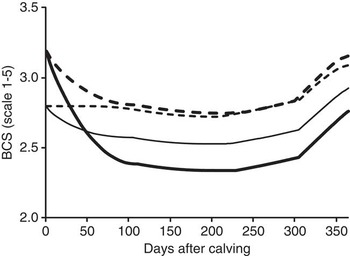
For each strain of HF cows, two BCS curves were simulated by defining BCS at calving at either 2.8 or 3.2 as inputs (Figure 8). This simulation shows the way in which BCS is genetically driven to the target BCS (BCS T and BCS at next calving, Table 1) set for each strain as it is conceptualised in the LIPID model.
Model simulations of BCS during lactation for North American Holstein–Friesian ( and —) and for New Zealand Holstein–Friesian cows (
 and - - -), calving with a BCS of either 3.2 or 2.80 (1 to 5 scale), respectively. Example for cows in second lactation, offered herbage allowance of 50 kg/cow per day, with 11.0 MJ/kg DM herbage, and offered no concentrates.

A genotype × environment interaction occurs when animals differ in their ability to perform in different environments (Falconer, Reference Falconer1981). Simulations depicted in Table 3 show that the e-Cow model is sensitive to genotype × environment interactions with regard to milksolids yield and milk yield. At low levels of feeding, that is, no concentrates offered, both strains performed similarly in terms of milksolids yield (kg MS/cow per lactation), but when 6 kg DM concentrates were offered, that is, higher level of feeding, NAHF produced more milksolids, as a consequence of their higher potential milk yield (Table 3).
Discussion
The e-Cow model allows the prediction of a dairy cow's performance at grazing, with and without supplementary feeding. The main features of the e-Cow model are the prediction of whole-lactation performance on a daily basis, the use of physical, metabolic and ingestive constraints in the prediction of herbage DM intake at grazing and the homeostatic and homeorhetic control of body lipid change. In addition, the e-Cow model is able to predict the performance of cows of different genetic merit and is able to account for genotype × environment interactions.
The model runs through a Visual Basic interface that requires one set of inputs related to feeds (several feeding periods can be created) and another set of inputs related to the cow. Feed-related inputs are HA, ME and NDF concentrations in herbage and supplements, amount of supplements offered and its efficiency of utilisation. The inputs related to the cow are pregnancy date, lactation number, BCS and LW at calving, breed or strain of cow and its genetic merit, that is, potential yields of milk, fat and protein. In addition, the user interface allows to define a dry-off policy and to edit some key parameters of the model.
Model validation
In validation tests, the e-Cow model showed satisfactory accuracy of prediction for herbage DM intake, milk yield and LW change (Table 2), and it compared well to the accuracy of prediction reported for similar models. Accuracy of prediction was lower for LW change than for other variables. This was also reported for other simulation models, and is possibly the result of greater experimental error in the measurements of LW than on other variables. Two other models, the animal model MOOSIM (Bryant et al., Reference Bryant, Lopez-Villalobos, Holmes, Pryce, Rossi and Macdonald2008) and the whole-farm model (WFM; Beukes et al., Reference Beukes, Palliser, Lancaster, Leydon-Davis, Levy, Folkers, Macdonald, Thorrold, Montgomierie and Wastney2006 and Reference Beukes, Palliser, Macdonald, Lancaster, Levy, Thorrold and Wastney2008) were also validated with the same dataset as the e-Cow model, but in all three cases, validation points were different. The WFM was validated for each HF strain separately and the validation points were annual values averaged per herd (3 years), the MOOSIM model was validated including both NA and NZ strain in the same dataset and the validation points were the daily values of individual cows in early lactation (1 year), while the e-Cow model was validated more intensively, with validation for each HF strain and for each parity separately, and the validation points were weekly values for the whole lactation (3 years).
Prediction of herbage intake, milk yield, LW and BCS
Other models can be used for grazing dairy cows. However, some of them were designed to formulate rations; thus, either expected milk yield or expected intake needs to be set as inputs and herbage availability or other restrictions at grazing are not accounted for (CNCPS, Fox et al., Reference Fox, Tedeschi, Tylutki, Russell, Amburgh, Chase, Pell and Overton2004; DAFOSYM, Rotz et al., Reference Rotz, Mertens, Buckmaster, Allen and Harrison1999). Other models do account for herbage availability, but do not include genetic drives in the prediction of BCS changes (GrazFeed, Freer et al., Reference Freer, Moore and Donnelly1997; DietCheck, Heard et al., Reference Heard, Cohen, Doyle, Wales and Stockdale2004).
The MOOSIM, the WFM and the e-Cow models account for animal requirements, herbage availability and restrictions at grazing to predict herbage DM intake, and they also account for genetic drives to predict changes in BCS. The MOOSIM and the WFM define the genetic merit of the cows based on their breeding values. In contrast, in the e-Cow model, the genetic merit of the cow is defined by the potential yields of milk, fat and protein, LW and parameters shown in Table 1 for BCS targets. This approach allows the model to be used for varying conditions across different countries, whereas in the case of using breeding values to define the genetic merit of the cow, the model is limited to the conditions in the country where the breeding values were estimated. However, in the e-Cow model, the parameters defining the initial genetically driven BCS curve (BCS, T and BCS next calving) used for different strains and parities require further testing.
In the e-Cow model, increments in the potential yields of the cow will only effect increments in DM intake when the metabolic limit is restricting intake, that is, the potential of the cow rather than the diet is limiting intake. However, it is possible, but not yet studied properly, that cows of higher genetic merit for milk yield may differ in their grazing ability from cows of lower genetic merit, which could be one of the reasons for their higher intake and higher milk yield at grazing when both are offered the same pasture allowance. In common with other previously published models, the e-cow model does not include any such differences in grazing ability, but they could be included if convincing evidence is produced in future studies.
The BCS of the cow affects DM intake at grazing in the e-Cow model, in as much as it affects the metabolic limit to potential DM intake. For example, assuming that cows A and B are the same and both the physical (PotDMIr) and the grazing limits (PotDMIg) to intake are higher than the metabolic limit (PotDMIe), if cow A loses more BCS, the e-Cow model predicts that cow A will have a lower intake than cow B.
As explained in the methodology section, the approach used here to define the potential yields in the e-Cow model was based on productions achieved by cows under experimental conditions, where feed quantity and quality were not limiting (no major nutritional limitations). However, this does not mean that the actual genetic merit of the cow is known, but it is a pragmatic approach to define potential genetic merit. The model uses default parameters (Table 1) to define the genetic potential of the cow; however, these parameters can be customised by using the buttons in the ‘genetic merit of the cow’ section of the input screen (Figure 4a).
The e-Cow model was validated against a dataset of cows grazing ryegrass-based pastures; however, the equations used to predict herbage DM intake of lucerne-based pastures were previously validated (Baudracco et al., Reference Baudracco, Lopez-Villalobos, Holmes, Brookes, Kemp, Comeron, Romero, Horan, Dillon and Berry2006).
Model simulations
The greater simulated milk response to concentrates by NAHF cows compared with that of NZHF (Figure 7) is consistent with independent experimental data (not used to develop or validate the e-Cow model) showing that high energy-demanding cows (high proportion of NA genes) have a greater response to supplements (Kennedy et al., Reference Kennedy, Dillon, Delaby, Faverdin, Stakelum and Rath2003; Kolver et al., Reference Kolver, Roche, Burke and Aspin2005; Fulkerson et al., Reference Fulkerson, Davison, Garcia, Hough, Goddard, Dobos and Blockey2008). This illustrates an important feature of e-Cow, which is its sensitivity to genotype × feeding environment interaction. These results agree with the results of Kolver et al. (Reference Kolver, Roche, Burke and Aspin2005), who compared both HF strains under feeding conditions similar to those used in the simulation shown in Table 3 and Figure 7.
A reason for the greater milk response to supplements in NAHF cows compared with NZHF cows is that NAHF have a higher relative feed deficit when grazing pastures (Penno et al., Reference Penno, Macdonald, Holmes, Davis, Wilson, Brookes and Thom2006; Holmes and Roche, Reference Holmes and Roche2007), and this results in a lower SR. The lower SRs predicted for NAHF cows occurred because the model sets a greater metabolic limit to intake for NAHF than NZHF cows (PotDMIe), given the higher potential milk yield of the former (effected by using different parameters for each strain in the MILK model). This lower SR of cows with a higher potential milk yield is more noticeable as the feeding level is increased.
In addition, as shown in Figure 7b, and reviewed elsewhere (Roche et al., Reference Roche, Friggens, Kay, Fisher, Stafford and Berry2009), high energy-demanding cows, that is, NAHF cows, mobilise more energy from body lipid reserves in early lactation, which is available for milk synthesis, and partition a greater proportion of energy consumed towards milk yield in mid and late lactation (effected by using different parameters for each strain in the LIPID model). Thus, cows with superior genetics for milk production have a depressed BCS profile (Roche et al., Reference Roche, Friggens, Kay, Fisher, Stafford and Berry2009), a consequence of the genetic correlation between these traits.
The inefficiencies occurring in grazing systems are accounted for in the e-Cow model by the calculated efficiency of grazing, which reports the proportion of herbage consumed relative to HA, the input ‘supplements efficiency of utilisation’ (Figure 4a), and coefficients of utilisation of ME energy for maintenance, milk yield, gestation and changes in BCS and LW.
Limitations of the e-Cow model
The e-Cow model is based on ME requirements, and it does not account for protein requirements. In addition, at the current stage of development, it does not include the effects of the environment, that is, weather conditions, on the performance of the cow. Heat stress can have detrimental effects on the milk yield and reproductive performance of dairy cows. Experimental data reporting a wide range of results on the effect of heat stress on cows of differing levels of milk yield may provide the parameters required for inclusion in the model.
The accuracy of prediction of the e-Cow may decrease for diets with less than 50% of pasture and high-quality supplements, because the potential DM intake is initially set for a whole-pasture diet. Further validation is required to test the model in high concentrate feeding scenarios. The prediction of changes in BCS for the whole lactation, performed with e-cow, agrees with published data for each of the two HF strains tested; however, the e-Cow model may not be accurate in the prediction of short-term changes in BCS across lactation. These limitations reflect the difficulty of simulation models in reproducing the complexity of the biological system.
In addition, the dataset used for the validation of e-Cow had a reduced range of supplementation levels, and, therefore, predictions for cows offered high levels of supplements may not be as accurate as those for cows offered low levels, as it may underestimate DM intake at high supplementation levels.
At the current stage of development, the e-Cow model does not relate pregnancy rate to BCS, but it could be linked in future work, by associating probabilities of pregnancy to levels of BCS.
The e-Cow model estimates DM intake based on an input HA, which can be calculated by the user from stocking rate and pre-grazing herbage mass. Further developments of the model will include the latter parameters as input variables. The empirical equations used to predict herbage DM intake at grazing could be replaced in future by more accurate equations, which could be obtained from future large grazing experiments with individual measurements of herbage DM intake at grazing.
Conclusions
The e-Cow model predicts, on a daily basis and for the whole lactation, herbage DM intake, milk yield and changes in BCS and LW for dairy cows at grazing, accounting for genetic differences between cows. In addition, it predicts body lipid change driven by both nutritional and genetic factors.
The e-Cow model was able to reproduce, with satisfactory accuracy, the differences observed in experiments for two strains of HF dairy cows, including the interaction between strains of HF cows and feeding environment. The approach used to define the potential milk yield of the cow and the equations used to predict herbage DM intake at grazing should allow the use of e-Cow in many countries with temperate pastures. This model is useful for applied research, teaching and extension purposes.
Acknowledgements
The authors thank Marcelo Zamateo for his support in the development of this model and Monika Zehetmeier for her suggestions.
Supplementary materials
The supplementary material referred to in this article is available online at http://www.journals.cambridge.org/anm