1. Introduction
In this paper we consider a mean-reverting process
 $(S_t)_{t\geq 0}$
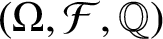
under a probability space
 $(\Omega ,\mathcal {F},\mathbb {Q})$
, described by the stochastic differential equation (SDE)
 $$ \begin{align} d S_t=\kappa(\mu(t)-\ln S_t)S_t\,d t+\sigma S_t\,d W_t, \end{align} $$
where
 $\kappa>0$
is the speed of the reversion,
 $\mu :[0,\infty )\rightarrow \mathbb {R}$
represents the long-run mean function of the process,
 $\sigma $
is the volatility, and
 $W_t$
is a standard Brownian motion driven on a filtration
 $(\mathcal {F}_t)_{t\geq 0}$
generated by the process.
The process satisfying model (1.1) generally represents the spot price of assets that exhibit mean reversion with both seasonal and nonseasonal behaviours, especially agricultural commodities, livestock, energy and manufactured metal. For a simple case of constant long-run mean functions, the model describes the price of nonseasonal mean-reverting assets, known as the one-factor Schwartz model. Schwartz [Reference Schwartz21] showed that it was suitable for the empirical price data of mean-reverting assets such as crude oil and copper. For a more complicated case, the seasonality of mean-reverting asset prices can be described by a periodic time-dependent long-run mean function
 $\mu (t)$
in the model. In addition, the model (1.1) was used to describe the short-term interest rate by Black and Karasinski [Reference Black and Karasinski2], called the Black–Karasinski model or extended exponential Vasicek model [Reference Brigo and Mercurio4].
Since all asset prices usually have fluctuations, financial derivatives such as futures and options are often used as tools to prevent risks for practitioners such as risk managers, investors and farmers. One of the most popular financial derivatives used for hedging the risks from price fluctuations is the European option [Reference Hull11], a financial contract which gives the buyer the right, but not the obligation, to buy (sell) an underlying asset at a predetermined price on a specific date. The option that gives the right to buy (sell) is called a call (put) option. The predetermined price of an underlying asset is called the strike price and the specific date is called the expiration date.
To enter a long or short position for an option, a premium or an option value must be determined under a particular assumption, known as the arbitrage-free condition. In other words, the price of an option must be fair for both seller and buyer. Consequently, the determination of the price for options is an important problem for researchers in the field of economics and mathematics [Reference Black1, Reference Black and Scholes3, Reference Chiu, Lo and Wong6, Reference Clewlow and Strickland8, Reference Merton14, Reference Swishchuk22, Reference Wong and Lo25].
Let
 $v(S,t;\phi )$
be the value of a European option on an underlying asset spot price S at time
 $t\leq T$
with a strike price K and an expiration date T, where
 $\phi =-1$
for a call option and
 $\phi =1$
for a put option. It is well known that under the risk-neutral measure, the fair value of the European option is
 $$ \begin{align} v(S,t;\phi) = e^{-r(T-t)} \mathbb{E}^{\mathbb{Q}} [ (\phi K-\phi S_T)^+|\mathcal{F}_t], \end{align} $$
where r is the constant risk-free interest rate.
The basic methods to approximate the European option value (1.2), such as Monte Carlo simulations and multinomial tree models, usually take considerable computation time.
Under model (1.1), we can show that the solution at the expiration time T with given initial time t is
 $$ \begin{align} S_T \,{=}\, &S_t^{e^{-\kappa (T-t)}} \exp \bigg\{ \frac{\sigma^2}{2\kappa} ( e^{-\kappa (T-t)} -1 ) + \kappa e^{-\kappa T} \int_{t}^{T} \mu(u) e^{\kappa u} \, d u + \sigma e^{-\kappa T} \int_{t}^{T} e^{\kappa u} \, d W_u \bigg\}, \end{align} $$
which has a log-normal distribution. One can compute the option price (1.2) by using the characteristic function approach (see [Reference Wong and Lo25] for more details); however, the formula obtained is in the form of an improper integral which is not easy to simplify and may take a long time to evaluate.
From the dynamics of the log-normal asset price, one can directly derive a closed-form formula for (1.2) by using the normal distribution property with the probability density function (PDF) of
 $\ln (S_T)$
. In this way, the formula obtained is similar to the Black–Scholes formula, where the more general mean and variance depend on the time to expiry; we refer to the resulting formula as a Black–Scholes-type formula. Although this probabilistic approach is effective for European options and the derivation is not complicated, it is not easy to apply and extend the idea for a more complicated option such as the American option, where the exercise time is not known [Reference Jacka12].
Alternatively, one powerful method that can handle both types of option is the partial differential equation (PDE) approach, where the problem of expectation is transformed into a PDE problem via the Feynman–Kac theorem [Reference Øksendal15]. For the European option, Chiu et al. [Reference Chiu, Lo and Wong6] used asymptotic expansions to approximate the solution of a PDE, under which the process follows a more general mean-reverting model with stochastic volatility. For the American option (on stocks), the reader can consult Kim [Reference Kim13], Underwood and Wang [Reference Underwood and Wang23], and Carr et al. [Reference Carr, Jarrow and Mynen5] for more details. Moreover, the PDE approach based on the Feynman–Kac theorem [Reference Øksendal15] was applied to price volatility derivatives as proposed in [Reference Chunhawiksit and Rujivan7, Reference Rujivan16–Reference Rujivan and Zhu20, Reference Weraprasertsakun and Rujivan24].
In the PDE approach, by applying the Feynman–Kac theorem [Reference Øksendal15] to model (1.1), the value of the European option (1.2) can be obtained from the solution of the PDE
 $$ \begin{align} \dfrac{\partial v(S,t;\phi)}{\partial t} +\frac{\sigma^2 S^2}{2} \dfrac{\partial^2 v(S,t;\phi)}{\partial S^2} +\kappa(\mu(t)-\ln S)S \dfrac{\partial v(S,t;\phi)}{\partial S} -r v(S,t;\phi) = 0, \end{align} $$
for
 $S>0$
and
 $0\leq t < T$
, subject to the terminal condition
 $$ \begin{align} v(S,T;\phi) = (\phi K-\phi S)^+, \quad S \geq 0. \end{align} $$
In this paper we propose a method for solving the PDE (1.4), subject to the terminal condition (1.5), in order to derive an analytical formula for pricing European options on the underlying asset whose prices follow model (1.1). To solve the PDE, we separate the solution into two parts, and apply the Fourier transform and method of characteristics to obtain the solution. The obtained formula can be expressed as the sum of the initial payoff of the option and the time-integral over the lifetime of the option.
The PDE approach developed in this paper has two main advantages: first, one can easily apply and modify the technique for more complicated pricing problems, for example, to obtain analytical formula for the American options under model (1.1); and second, the decomposition of the solution can be used to approximate the option price using the known initial payoff and the approximation of the integral term.
The rest of this paper is organized as follows. Section 2 provides details on deriving an analytical formula for pricing European options on a mean-reverting asset whose prices satisfy the model (1.1). Section 3 gives the derivation of the Black–Scholes-type formula, and demonstrates numerical results of the option values computed from the formula under various kinds of long-run mean functions. Comparisons of our results with Monte Carlo simulations and the Black–Scholes-type formula, and the behaviours of option prices, are also illustrated in this section. Section 4 concludes.
2. An integral representation for European options
In this section we give an integral representation formula for pricing the European option on a mean-reverting asset whose prices satisfy model (1.1). In addition, the put–call parity formula for the European option is provided.
In order to derive our formula, we need the boundary conditions for
 $v(S,t;\phi )$
provided in the following lemma.
Lemma 2.1. Assume that the underlying asset spot price
 $(S_t)_{t\geq 0}$
follows model (1.1) with integrable function
 $\mu :[0,T]\rightarrow \mathbb {R}$
. Then
 $$ \begin{align} \lim_{S\rightarrow0} v(S,t;-1) =\lim_{S\rightarrow\infty} v(S,t;1) = 0 , \end{align} $$
for
 $0\leq t < T$
.
Proof. Let
 $X_t = \ln S_t$
. By Itô’s lemma, model (1.1) can be written as the extended Vasicek model [Reference Hull and White10]
 $$ \begin{align} d X_t=\kappa(\alpha(t) - X_t)\,d t+\sigma \,d W_t, \end{align} $$
where
 $\alpha (t) = \mu (t) - \sigma ^2/2\kappa $
, and the solution of (2.2) is
 $$ \begin{align*} X_t = X_0 e^{-\kappa t} + \kappa e^{-\kappa t} \int_{0}^{t} \alpha(u) e^{\kappa u} \, d u +\sigma e^{-\kappa t} \int_{0}^{t} e^{\kappa u} \, d W_u. \end{align*} $$
Hence, the solution to (1.1) is
 $$ \begin{align*} S_t = S_0^{e^{-\kappa t}} \exp \bigg\{ \frac{\sigma^2}{2\kappa} ( e^{-\kappa t} -1 ) + \kappa e^{-\kappa t} \int_{0}^{t} \mu(u) e^{\kappa u} \, d u + \sigma e^{-\kappa t} \int_{0}^{t} e^{\kappa u} \, d W_u \bigg\}. \end{align*} $$
It is easy to see from integrability of
 $\mu $
that the term
 $$\begin{align*}\frac{\sigma^2}{2\kappa} ( e^{-\kappa t} -1 ) + \kappa e^{-\kappa t} \int_{0}^{t} \mu(u) e^{\kappa u} \, d u + \sigma e^{-\kappa t} \int_{0}^{t} e^{\kappa u} \, d W_u \end{align*}$$
is bounded for all
 $0\leq t < T$
. Thus, the condition
 $$ \begin{align} S_t \rightarrow 0 \text{ for some } 0\leq t < T \text{ implies } S_T \rightarrow 0 \text{ as well. } \end{align} $$
By (1.2), for
 $0\leq t < T ,$
 $$ \begin{align} \lim_{S\rightarrow0} v(S,t;-1) &= \lim_{S\rightarrow0} e^{-r(T-t)} \mathbb{E}^{\mathbb{Q}} [ (S_T - K)^+|\mathcal{F}_t] \notag\\ &= e^{-r(T-t)} \mathbb{E}^{\mathbb{Q}} [ (S_T - K)^+|S_T \rightarrow 0 ] \notag\\ &=0. \end{align} $$
Similar to (2.3), the condition
 $$ \begin{align*} S_t \rightarrow \infty \text{ for some } 0\leq t < T \text{ implies } S_T \rightarrow \infty. \end{align*} $$
Similar to (2.4),
 $\displaystyle \lim \nolimits _{S\rightarrow \infty } v(S,t;1) = \lim \nolimits _{S\rightarrow \infty } e^{-r(T-t)} \mathbb {E}^{\mathbb {Q}} [ ( K - S_T)^+|\mathcal {F}_t] =0. $
The analytical formula for European options is now derived by solving the PDE (1.4) subject to the terminal condition (1.5) as described in the following theorem.
Theorem 2.2. Assume that
 $\mu :[0,T]\rightarrow \mathbb {R}$
is integrable. Then the value of a European option
 $v(S,t;\phi )$
on the asset spot price S at time
 $t\leq T$
with a strike price K and an expiration date T is represented by
 $$ \begin{align} {v}(S,t;\phi) = \widetilde{u}(S,T-t;\phi) +(\phi K-\phi S)^+, \end{align} $$
where
 $$ \begin{align} \widetilde{u}(S,\tau;\phi) &= \int_{0}^{\tau} \{ K ( H_1 + \phi H_2 \, \mathcal{N} [ \phi d_1(\rho) ] ) +S^{e^{-\kappa\rho}} M ( H_3 +\phi H_4 \, \mathcal{N} [ \phi d_2(\rho) ] ) \} \,d \rho , \end{align} $$
with
 $$ \begin{align*} H_1 &= \frac{\sigma \sqrt{\kappa} e^{(\kappa-r)\rho- d_1^2(\rho)/2} }{2\sqrt{\pi}\sqrt{e^{2\kappa\rho}-1}}, \notag\\ H_2 &= - r e^{-r\rho} , \notag\\ H_3 &= - \frac{\sigma \sqrt{\kappa} }{2\sqrt{\pi}} ( \sqrt{e^{2\kappa\rho }-1} ) e^{- d_2^2(\rho)/2}, \notag\\ H_4 &= ( r-\kappa\mu(T-\tau+\rho) ) e^{\kappa\rho} + \kappa\ln S + \frac{\sigma^2}{2} ( 1- e^{-\kappa\rho} ) + \kappa \varphi(\rho) , \notag\\ M &= \exp \bigg( -(r + \kappa)\rho - \frac{\sigma^2}{4\kappa} (1-e^{-\kappa\rho} )^2 + e^{-\kappa\rho} \varphi(\rho) \bigg), \notag\\ d_1(\rho) &= \frac{\sqrt{2\kappa}}{\sigma\sqrt{e^{2\kappa\rho} -1}} \bigg\{ \ln\frac{K}{S} +\bigg(\frac{\sigma^2}{2\kappa} +\ln K \bigg) ( e^{\kappa\rho}-1 ) - \varphi(\rho) \bigg\}, \notag\\ d_2(\rho) &= d_1(\rho) -\dfrac{\sigma \sqrt{1-e^{-2\kappa\rho}}}{\sqrt{2\kappa}}, \notag\\ \varphi(\rho) &= \kappa e^{\kappa\tau} \int_{\tau-\rho}^{\tau} \mu(T-w)e^{-\kappa w} \, d w , \end{align*} $$
and
 $\mathcal {N}[\cdot ]$
as the cumulative distribution function (CDF) of the standard normal distribution.
Proof. For ease of notation, we write
 $v(S,t)$
for
 $v(S,t;\phi )$
in the proof. This proof is divided into three parts: (i) conversion and Fourier transform; (ii) inversion; and (iii) solution.
-
(i) Conversion and Fourier transform.
Note that the domain of the European option value
 $v(S,t)$
is First, we change variables as follows:
$$ \begin{align*} \{(S,t)\mid 0< S <\infty,\, 0\leq t \leq T\}. \end{align*} $$
(2.7)Then the new domain is
$$ \begin{align} \tau := T-t, \quad x := -\ln S, \quad \widetilde{\mu}(\tau) := \mu(t), \quad E(x,\tau) := v(S,t). \end{align} $$
$\{(x,\tau )\mid x\in \mathbb {R}, 0\leq \tau \leq T\}$
. By the chain rule, Substituting into (1.4), we obtain a new PDE
$$ \begin{align*} \dfrac{\partial v(S,t)}{\partial t} &= -\dfrac{\partial E(x,\tau)}{\partial \tau} , \quad \dfrac{\partial v(S,t)}{\partial S} =-\frac{1}{S} \dfrac{\partial E(x,\tau)}{\partial x}, \\ \dfrac{\partial^2 v(S,t)}{\partial S^2} &=\frac{1}{S^2}\dfrac{\partial^2 E(x,\tau)}{\partial x^2} +\frac{1}{S^2}\dfrac{\partial E(x,\tau)}{\partial x}. \end{align*} $$
(2.8)where
$$ \begin{align} \mathcal{L} E(x,\tau) = 0, \quad x\in\mathbb{R},\, 0< \tau \leq T, \end{align} $$
By (2.7), the terminal condition (1.5) becomes the initial condition
$$ \begin{align*} \mathcal{L}= \dfrac{\partial }{\partial \tau} -\frac{\sigma^2}{2}\dfrac{\partial^2 }{\partial x^2} +\bigg( -\frac{\sigma^2}{2} +\kappa\widetilde{\mu}(\tau) +\kappa x \bigg) \dfrac{\partial }{\partial x} +r. \end{align*} $$
(2.9)and the boundary conditions (2.1) become
$$ \begin{align} E(x,0) = (\phi K - \phi e^{-x})^+, \end{align} $$
(2.10)
$$ \begin{align} \lim_{x\rightarrow\infty} E(x,\tau) &= 0 \quad \text{if } \phi=-1, \nonumber\\ \lim_{x\rightarrow-\infty} E(x,\tau) &= 0 \quad \text{if } \phi=1. \end{align} $$
To solve the PDE (2.8) subject to (2.9)–(2.10), we apply ideas of Underwood and Wang [Reference Underwood and Wang23] by setting
(2.11)where
$$ \begin{align} E(x,\tau) = u(x,\tau) +g(x),\quad x\in\mathbb{R},\, 0\leq \tau \leq T, \end{align} $$
(2.12)Substituting (2.11) into (2.8) and (2.9)–(2.10), we have the new PDE
$$ \begin{align} g(x) &= (\phi K - \phi e^{-x})^+. \end{align} $$
(2.13)where
$$ \begin{align} \mathcal{L} u(x,\tau) = f(x,\tau), \quad x\in\mathbb{R},\, 0< \tau \leq T, \end{align} $$
(2.14)with the initial condition
$$ \begin{align} f(x,\tau) = -\mathcal{L} g(x) , \end{align} $$
(2.15)and the boundary condition
$$ \begin{align} u(x,0) &= 0, \end{align} $$
(2.16)
$$ \begin{align} \lim_{\phi x\rightarrow-\infty} u(x,\tau) &= \lim_{\phi x\rightarrow-\infty} ( E(x,\tau) - g(x) ) = - \lim_{\phi x\rightarrow-\infty} (\phi K - \phi e^{-x})^+ = 0. \end{align} $$
We now apply the Fourier transform to solve (2.13), subject to conditions (2.15)–(2.16). The Fourier transform in x of a function
$h(x,\tau )$
is defined by and note that
$$\begin{align*}H(\xi,\tau) = \mathcal{F}[h(x,\tau)] = \dfrac{1}{\sqrt{2\pi}}\int_{-\infty}^{\infty} h(x,\tau)e^{i\xi x} \, d x, \end{align*}$$
Using these facts and taking the Fourier transform of the PDE (2.13) and the initial condition (2.15), we obtain a first-order linear PDE
$$ \begin{align*} \mathcal{F}\bigg[\dfrac{\partial h(x,\tau)}{\partial x}\bigg] &= -i\xi H(\xi,\tau), \quad \mathcal{F}\bigg[\dfrac{\partial^2 h(x,\tau)}{\partial x^2}\bigg] = -\xi^2 H(\xi,\tau), \\ \mathcal{F}\bigg[x \dfrac{\partial h(x,\tau)}{\partial x}\bigg] &= -\xi \dfrac{\partial H(\xi,\tau)}{\partial \xi}-H(\xi,\tau). \end{align*} $$
(2.17)for
$$ \begin{align} \dfrac{\partial U(\xi,\tau)}{\partial \tau} -\kappa\xi \dfrac{\partial U(\xi,\tau) }{\partial \xi} +A(\xi,\tau)U(\xi,\tau) = F(\xi,\tau) \end{align} $$
$\xi \in \mathbb {R},\, 0< \tau \leq T$
, with the initial condition (2.18)where
$$ \begin{align} U(\xi,0) = \mathcal{F}[u(x,0)] = 0, \end{align} $$
$F(\xi ,\tau ) := \mathcal {F}[f(x,\tau )]$
and (2.19)
$$ \begin{align} A(\xi,\tau) &= \frac{\sigma^2}{2}\xi^2 +\bigg( \frac{\sigma^2}{2} -\kappa\widetilde{\mu}(\tau) \bigg) i\xi +r -\kappa. \end{align} $$
To solve this PDE, we apply the method of characteristics. We set
with parametric equations
$$ \begin{align*}\xi\equiv\xi(s), \!\quad\! \tau \equiv \tau(s),\!\quad\! U(\xi,\tau) \equiv U(\xi(s), \!\quad\! \tau(s)) \equiv U(s),\!\quad\! (\xi(0),\tau(0)) =(\xi_0,0)\end{align*} $$
where s is a parameter. Then the PDE (2.17) becomes a first-order linear ordinary differential equation
$$ \begin{align*} \tau(s) = s, \quad \xi(s) =\xi_0e^{-\kappa \tau(s)} =\xi_0e^{-\kappa s}, \end{align*} $$
(2.20)Solving (2.20) yields
$$ \begin{align} \frac{d U(s) }{d s } +A(\xi_0e^{-\kappa s},s ) U(s) = F(\xi_0e^{-\kappa s},s ). \end{align} $$
(2.21)Substituting
$$ \begin{align} U(s ) = e^{- \int_{0}^{s} A(\xi_0e^{-\kappa z},z) \, dz} \bigg\{ \displaystyle\int_{0}^{s} e^{\int_{0}^{\hat{\tau}} A(\xi_0e^{-\kappa z},z) \, dz } F(\xi_0e^{-\kappa \hat{\tau}},\hat{\tau}) \, d\hat{\tau} +U(0) \bigg\}. \end{align} $$
$s = \tau $
and
$\xi _0 = \xi e^{\kappa \tau }$
back into (2.21) and using the initial condition (2.18), we have (2.22)where
$$ \begin{align} U(\xi,\tau ) &=e^{- \int_{0}^{\tau} A(\xi e^{\kappa\tau-\kappa z},z) \, dz} \bigg\{ \displaystyle\int_{0}^{\tau} e^{\int_{0}^{\hat{\tau}} A(\xi e^{\kappa\tau-\kappa z},z) \, dz } F(\xi e^{\kappa\tau-\kappa \hat{\tau}},\hat{\tau}) \, d\hat{\tau} +U(\xi_0,0) \bigg\} \notag\\ &= \displaystyle\int_{0}^{\tau} e^{\hat{B}(\xi,\tau,\hat{\tau}) -\hat{B}(\xi,\tau,\tau) } F(\xi e^{\kappa\tau-\kappa \hat{\tau}},\hat{\tau}) \, d\hat{\tau} \notag\\ &= \int_{0}^{\tau} F_1(\xi,\tau,\hat{\tau}) F(\xi e^{\kappa (\tau-\hat{\tau})},\hat{\tau}) \, d\hat{\tau} , \end{align} $$
From (2.19),
$$ \begin{align*}\hat{B}(\xi,\tau,y) = \int_{0}^{y} A(\xi e^{\kappa\tau-\kappa z},z) \, dz, \quad \text{ and }\quad F_1(\xi,\tau,\hat{\tau}) = e^{\hat{B}(\xi,\tau,\hat{\tau}) -\hat{B}(\xi,\tau,\tau) }.\end{align*} $$
and
$$ \begin{align*} \hat{B}(\xi,\tau,y) &= \frac{\sigma^2 e^{2\kappa \tau} (1-e^{-2\kappa y} )}{4\kappa} \xi^2 +\frac{\sigma^2}{2\kappa} i\xi e^{\kappa\tau} (1-e^{-\kappa y}) \notag\\ &\quad - \kappa i\xi e^{\kappa\tau} \int_{0}^{y} \widetilde{\mu}(z)e^{-\kappa z} \, dz+ (r -\kappa ) y, \end{align*} $$
(2.23)
$$ \begin{align} F_1(\xi,\tau,\hat{\tau}) &= \exp \bigg\{ (r -\kappa )(\hat{\tau} - \tau) + \frac{\sigma^2 ( 1- e^{2\kappa (\tau-\hat{\tau})} )}{4\kappa} \xi^2 \notag\\ &\quad + i\xi \bigg( \frac{\sigma^2 ( 1- e^{\kappa (\tau-\hat{\tau})} )}{2\kappa} + \kappa e^{\kappa\tau} \int_{\hat{\tau}}^{\tau} \widetilde{\mu}(z)e^{-\kappa z} \, dz \bigg) \bigg\}. \end{align} $$
-
(ii) Inversion.
Note that, when
$h =\mathcal {F}^{-1} [H(\xi )] $
, the scaling property of Fourier transform gives (2.24)for every
$$ \begin{align} \mathcal{F}^{-1}[H(c\xi )] = \frac{1}{|c|} h\bigg(\frac{x}{c}\bigg) \end{align} $$
$c\in \mathbb {R}\backslash \{0\}$
. From (2.24) and the convolution property, (2.25)
$$ \begin{align} \mathcal{F}^{-1}[H_1(\xi )H_2(c\xi )] &= \dfrac{1}{\sqrt{2\pi}} ( \mathcal{F}^{-1}[H_1(\xi )]*\mathcal{F}^{-1}[H_2(c\xi )] ) \notag\\[1pt] &= \dfrac{1}{|c|\sqrt{2\pi}} \int_{-\infty}^{\infty} h_1 (x-z) h_2 \bigg(\frac{z}{c}\bigg) \, dz \end{align} $$
for every
$c\in \mathbb {R}\backslash \{0\}$
,
$h_1 = \mathcal {F}^{-1} [H_1(\xi )]$
, and
$h_2 = \mathcal {F}^{-1} [H_2(\xi )]$
. By applying (2.25) with
$c=e^{\kappa (\tau -\hat {\tau })}$
and taking the inverse transform of (2.22), (2.26)where
$$ \begin{align} u(x,\tau) &= \mathcal{F}^{-1}[U(\xi,\tau )] = \int_{0}^{\tau} \mathcal{F}^{-1} [ F_1(\xi,\tau,\hat{\tau}) F(\xi e^{\kappa(\tau-\hat{\tau})},\hat{\tau}) ] \,d\hat{\tau} \notag\\ &= \dfrac{1}{\sqrt{2\pi}} \int_{0}^{\tau} e^{\kappa(\hat{\tau}- \tau) } \int_{-\infty}^{\infty} f_1(x-z,\tau,\hat{\tau}) f(z e^{\kappa(\hat{\tau}- \tau) } ,\hat{\tau})\, d z \, d \hat{\tau} , \end{align} $$
$f_1(x,\tau ,\hat {\tau }) = \mathcal {F}^{-1}[F_1(\xi ,\tau ,\hat {\tau })] $
. From the integral of the Gaussian function equation (2.23) yields
$$ \begin{align*} \int_{-\infty}^{\infty} e^{-\hat{a} y^2 +\hat{b}y+\hat{c}} \, dy = e^{\hat{b}^2/4\hat{a}+\hat{c}}\sqrt{\frac{\pi}{\hat{a}}} ,\end{align*} $$
(2.27)when
$$ \begin{align} f_1(x,\tau,\hat{\tau}) &= \mathcal{F}^{-1}[F_1(\xi,\tau,\hat{\tau})] = \frac{1}{\sqrt{2\pi}} \int_{-\infty}^{\infty} F_1(\xi,\tau,\hat{\tau})e^{-i\xi x} \, d\xi \notag\\ &= \frac{\sqrt{2\kappa}\, e^{(r-\kappa)(\hat{\tau}-\tau)}}{\sigma\sqrt{ e^{2\kappa (\tau-\hat{\tau})} -1 }}\notag\\ &\quad\times\exp \bigg\{ \frac{ -\{ (\sigma^2/2\kappa) ( 1- e^{\kappa (\tau-\hat{\tau})} ) + \kappa e^{\kappa\tau} \int_{\hat{\tau}}^{\tau} \widetilde{\mu}(w)e^{-\kappa w} \, dw -x \}^2}{\sigma^2 (e^{2\kappa (\tau-\hat{\tau})} -1 )/\kappa } \bigg\} , \end{align} $$
and
$$ \begin{align*}\hat{a} = \frac{\sigma^2 (e^{2\kappa (\tau-\hat{\tau})} -1 ) }{4\kappa} , \quad \hat{b} = i\, \bigg( \frac{\sigma^2 ( 1- e^{\kappa (\tau-\hat{\tau})} ) }{2\kappa} + \kappa e^{\kappa\tau} \int_{\hat{\tau}}^{\tau} \widetilde{\mu}(w)e^{-\kappa w} \, dw -x \bigg) ,\end{align*} $$
$\hat {c} = (r-\kappa )(\hat {\tau }-\tau )$
. From (2.12), we can write (2.28)where
$$ \begin{align} g(x) &= (\phi K - \phi e^{-x}) \mathbf{1}_{\{\phi x\geq - \phi\ln K\}}(x), \end{align} $$
$\mathbf {1}_{\{\phi x\geq - \phi \ln K\}}(\cdot )$
is the indicator function [Reference Folland9]. Thus (2.29)where
$$ \begin{align} \dfrac{\partial g(x)}{\partial x} &=\phi e^{-x} \mathbf{1}_{\{\phi x\geq - \phi\ln K\}}(x) , \nonumber\\ \dfrac{\partial^2 g(x)}{\partial x^2} &= K\delta ( x+\ln K ) - \phi e^{-x} \mathbf{1}_{\{\phi x\geq - \phi\ln K\}}(x) , \end{align} $$
$\delta (\cdot ) $
is the Dirac delta function. By substituting (2.28)–(2.29) into (2.14), (2.30)Using (2.27) and (2.30), we rewrite (2.26) in the form
$$ \begin{align} f(x,\tau) &= \frac{\sigma^2 K}{2} \, \delta ( x+\ln K ) + \phi ( (r-\kappa\widetilde{\mu}(\tau) -\kappa x) e^{-x} -rK ) \mathbf{1} _{\{\phi x\geq - \phi\ln K\}}(x). \end{align} $$
(2.31)where
$$ \begin{align} u(x,\tau) &= \int_{0}^{\tau} \int_{-\infty}^{\infty} f_3(x-z,\tau,\hat{\tau}) f_2(z ,\tau,\hat{\tau}) \, d z \, d \hat{\tau} , \end{align} $$
(2.32)
$$ \begin{align} f_2(z,\tau,\hat{\tau}) &= e^{r(\hat{\tau}- \tau)} f(z e^{\kappa(\hat{\tau}- \tau)} ,\hat{\tau}) \notag\\ &= \frac{\sigma^2K e^{(r-\kappa)(\hat{\tau}- \tau)}}{2} \, \delta ( z + e^{\kappa(\tau-\hat{\tau})}\ln K ) + \phi ( ( r-\kappa\widetilde{\mu}(\hat{\tau}) ) e^{r(\hat{\tau}- \tau)-z e^{\kappa(\hat{\tau}- \tau)}} \notag\\ &\quad - \kappa z e^{(r+\kappa)(\hat{\tau}- \tau)-z e^{\kappa(\hat{\tau}- \tau)}} - rK e^{r(\hat{\tau}- \tau)} ) \mathbf{1} _{\{ \phi z \geq -\phi e^{\kappa( \tau-\hat{\tau})} \ln K \}}(z), \end{align} $$
(2.33)
$$ \begin{align} f_3(x,\tau,\hat{\tau}) &= \dfrac{e^{(\kappa-r)(\hat{\tau}- \tau) }}{\sqrt{2\pi}} f_1(x,\tau,\hat{\tau}) \notag\\ &= \dfrac{1}{\sqrt{2\pi}} \bigg( \frac{\sigma\sqrt{ e^{2\kappa (\tau-\hat{\tau})} -1 }}{\sqrt{2\kappa}} \bigg)^{-1} \notag\\ & \quad \times \exp\bigg\{ \frac{ -\{ x +(\sigma^2/2\kappa) ( e^{\kappa (\tau-\hat{\tau})} -1 ) - \kappa e^{\kappa\tau} \int_{\hat{\tau}}^{\tau} \widetilde{\mu}(w)e^{-\kappa w} \, dw \}^2}{2( \sigma\sqrt{ e^{2\kappa (\tau-\hat{\tau})} -1 }/\sqrt{2\kappa} )^2} \bigg\}. \end{align} $$
-
(iii) Solution.
Note that
(2.34)for any integrable function h, and
$$ \begin{align} \int_{-\infty}^{\infty}h(z) \mathbf{1} _{\{ \phi z \geq \phi m \}}(z)\, d z = \lim_{\phi n\rightarrow\infty} \phi \int_{m}^{n}h(z) \, d z \end{align} $$
$m\in \mathbb {R}$
. From (2.31)–(2.33), by applying (2.34) to (2.32), we can write the solution in the form (2.35)where
$$ \begin{align} u(x,\tau) =& \int_{0}^{\tau}( I_1+I_2+I_3+I_4 ) \,d \hat{\tau} , \end{align} $$
(2.36)
$$ \begin{align} I_1 &= \int_{-\infty}^{\infty} \frac{\sigma^2K e^{(r-\kappa)(\hat{\tau}- \tau)}}{2} \, \delta ( z + e^{\kappa(\tau-\hat{\tau})}\ln K ) \, f_3(x-z,\tau,\hat{\tau}) \,d z, \end{align} $$
(2.37)For convenience, we denote
$$ \begin{align} I_2 & = \lim_{\phi n\rightarrow\infty} \int_{-e^{\kappa( \tau-\hat{\tau})} \ln K}^{n} ( r-\kappa\widetilde{\mu}(\hat{\tau}) ) e^{r(\hat{\tau}- \tau)-z e^{\kappa(\hat{\tau}- \tau)}} f_3(x-z,\tau,\hat{\tau}) \,d z, \\ I_3 & = -\lim_{\phi n\rightarrow\infty} \int_{-e^{\kappa( \tau-\hat{\tau})} \ln K}^{n} \kappa z e^{(r+\kappa)(\hat{\tau}- \tau)-z e^{\kappa(\hat{\tau}- \tau)}} f_3(x-z,\tau,\hat{\tau}) \,d z, \nonumber \\ I_4 & = -\lim_{\phi n\rightarrow\infty} \int_{-e^{\kappa( \tau-\hat{\tau})} \ln K}^{n} rK e^{r(\hat{\tau}- \tau)}f_3(x-z,\tau,\hat{\tau}) \,d z. \nonumber \end{align} $$
(2.38)From (2.33), (2.36) and (2.38),
$$ \begin{align} \left\{ \begin{array}{lll} a = e^{\kappa(\tau-\hat{\tau})},& b = \dfrac{\sigma^2}{2\kappa} ( e^{\kappa (\tau-\hat{\tau})} -1 ) - \kappa e^{\kappa\tau}\displaystyle \int_{\hat{\tau}}^{\tau} \widetilde{\mu}(w)e^{-\kappa w} \, dw, \\ c = \dfrac{\sigma\sqrt{e^{2\kappa(\tau-\hat{\tau})}-1}}{\sqrt{2\kappa}}, & m = -e^{\kappa( \tau-\hat{\tau})} \ln K. \end{array} \right. \end{align} $$
(2.39)By (2.33), (2.37) and (2.38),
$$ \begin{align} I_1 &= \frac{\sigma^2K e^{(r-\kappa)(\hat{\tau}- \tau)}}{2} f_3 ( x+e^{\kappa( \tau-\hat{\tau})} \ln K,\tau,\hat{\tau} ) = \frac{\sigma^2K e^{(r-\kappa)(\hat{\tau}- \tau)}}{2} f_3 ( x-m,\tau,\hat{\tau} ) \notag\\ &= \frac{\sigma^2K }{2c\sqrt{2\pi}} \exp\bigg\{ (r-\kappa)(\hat{\tau}- \tau) -\frac{1}{2}\bigg(\frac{ x-m+b }{c}\bigg)^2 \bigg\}. \end{align} $$
(2.40)where
$$ \begin{align} I_2 &= ( r-\kappa\widetilde{\mu}(\hat{\tau}) )e^{r(\hat{\tau}- \tau)}J_2 , \end{align} $$
(2.41)
$$ \begin{align} J_2 &= \lim_{\phi n\rightarrow\infty} \int_{m}^{n}e^{-z/a} f_3(x-z,\tau,\hat{\tau}) \,d z\notag\\ &= \lim_{\phi n\rightarrow\infty} \bigg( \frac{1}{c\sqrt{2\pi}} \int_{m}^{n} \exp\bigg\{ -\frac{z}{a} -\frac{1}{2}\bigg(\frac{ x-z+b }{c}\bigg)^2 \bigg\}\,d z\bigg)\notag\\ &= \exp \bigg\{ \frac{-x-b+c^2/2a}{a} \bigg\}\notag\\ &\quad \times \lim_{\phi n\rightarrow\infty} \bigg(\frac{1}{c\sqrt{2\pi}} \int_{m}^{n} \exp\bigg\{ -\frac{1}{2}\bigg(\frac{ z -x-b+c^2/a}{c}\bigg)^2 \bigg\}\,d z \bigg) \end{align} $$
(2.42)Recall that the CDF of the standard normal distribution is defined by
$$ \begin{align} &= \exp \bigg\{ \frac{-x-b+c^2/2a}{a} \bigg\} \lim_{\phi n\rightarrow\infty} \bigg( \frac{1}{\sqrt{2\pi}} \int_{({m-x-b+c^2/a})/{c}}^{({n-x-b+c^2/a})/{c}} e^{-y^2/2}\,d y \bigg). \end{align} $$
(2.43)Applying (2.43) to (2.42) yields
$$ \begin{align} \mathcal{N}[z] := \frac{1}{\sqrt{2\pi}} \int_{-\infty}^{z} e^{-y^2/2} \,d y. \end{align} $$
(2.44)Thus,
$$ \begin{align} J_2 &=\phi \exp \bigg\{ \frac{-x-b+c^2/2a}{a} \bigg\} \mathcal{N}\bigg[ -\phi \bigg( \frac{m-x-b+c^2/a}{c} \bigg) \bigg]. \end{align} $$
(2.45)Similarly to the way we obtain (2.40)–(2.41), we set
$$ \begin{align} I_2 &= \phi ( r-\kappa\widetilde{\mu}(\hat{\tau}) ) \exp \bigg\{ r(\hat{\tau}- \tau) +\frac{-x-b+c^2/2a}{a} \bigg\} \notag\\ &\quad \times \mathcal{N}\bigg[ -\phi \bigg( \frac{m-x-b+c^2/a}{c} \bigg) \bigg]. \end{align} $$
(2.46)where
$$ \begin{align} I_3 &= -\frac{\kappa e^{r(\hat{\tau}- \tau)}}{a}\lim_{\phi n\rightarrow\infty} \int_{m}^{n} z e^{-z/a} f_3(x-z,\tau,\hat{\tau}) \,d z \notag\\ &= -\frac{\kappa}{a}\exp \bigg\{ r(\hat{\tau}- \tau) + \frac{-x-b+c^2/2a}{a} \bigg\}J_3 , \end{align} $$
(2.47)Similar to (2.42), applying (2.43) and setting
$$ \begin{align} J_3 = \lim_{\phi n\rightarrow\infty} \bigg[ \frac{1}{c\sqrt{2\pi}} \int_{m}^{n} z \exp\bigg\{ -\frac{1}{2}\bigg(\frac{ z -x-b+c^2/a}{c}\bigg)^2 \bigg\}\, dz \bigg]. \end{align} $$
$h = -x-b+c^2/a $
in (2.47), we have (2.48)Substituting (2.48) into (2.46) yields
$$ \begin{align} J_3 &= \lim_{\phi n\rightarrow\infty} \bigg[ \frac{1}{c\sqrt{2\pi}} \int_{m}^{n} ( z+h) \exp\bigg\{ -\frac{1}{2}\bigg(\frac{ z +h}{c}\bigg)^2 \bigg\}\,d z \notag\\ &\quad - \frac{h}{c\sqrt{2\pi}} \int_{m}^{n} \exp\bigg\{ -\frac{1}{2}\bigg(\frac{ z +h}{c}\bigg)^2 \bigg\}\, dz \bigg] \notag\\ &= \frac{c}{\sqrt{2\pi}} \exp \bigg\{-\frac{1}{2}\bigg(\frac{m+h}{c}\bigg)^2 \bigg\}- \phi h \mathcal{N}\bigg[ -\phi \bigg(\frac{m+h}{c} \bigg) \bigg]. \end{align} $$
(2.49)
$$ \begin{align} I_3 &= -\frac{\kappa c}{a\sqrt{2\pi}} \exp \bigg\{ r(\hat{\tau}- \tau) + \frac{-x-b+c^2/2a}{a} - \frac{1}{2}\bigg(\frac{m-x-b+c^2/a}{c}\bigg)^2\bigg\}\notag\\ &\quad -\phi \kappa \bigg( \frac{ x+b-c^2/a}{a} \bigg) \exp \bigg\{ r(\hat{\tau}- \tau) + \frac{-x-b+c^2/2a}{a} \bigg\}\notag\\ &\quad \times \mathcal{N}\bigg[ -\phi \bigg( \frac{m-x-b+c^2/a}{c} \bigg) \bigg]. \end{align} $$
Similarly to (2.44), using the normal distribution function and (2.33), we obtain
(2.50)Collecting (2.35), (2.39), (2.45), and (2.49)–(2.50) after combining
$$ \begin{align} I_4 &= -\phi rK e^{r(\hat{\tau}- \tau)} \mathcal{N}\bigg[ -\phi \bigg( \frac{m-x-b}{c} \bigg) \bigg]. \end{align} $$
$I_2$
and
$I_3$
, we obtain (2.51)Substituting
$$ \begin{align} u(x,\tau) & = \int_{0}^{\tau}\bigg\{\frac{\sigma^2K }{2c\sqrt{2\pi}} \exp\bigg\{ (r-\kappa)(\hat{\tau}- \tau) -\frac{1}{2}\bigg(\frac{ x-m+b }{c}\bigg)^2 \bigg\} \notag\\ &\quad -\phi rK e^{r(\hat{\tau}- \tau)} \mathcal{N}\bigg[ \phi \bigg( \frac{x-m+b}{c} \bigg) \bigg] \notag\\ &\quad -\frac{\kappa c}{a\sqrt{2\pi}} \exp \bigg\{ r(\hat{\tau}- \tau) + \frac{-x-b+c^2/2a}{a} - \frac{1}{2}\bigg(\frac{x-m+b-c^2/a}{c}\bigg)^2\bigg\} \notag\\ &\quad +\phi \bigg(r -\kappa\widetilde{\mu}(\hat{\tau}) +\kappa \bigg( \frac{ -x-b+c^2/a}{a} \bigg) \bigg) \notag\\ & \quad \times \exp \bigg\{ r(\hat{\tau}- \tau) + \frac{-x-b+c^2/2a}{a} \bigg\} \mathcal{N}\bigg[ \phi \bigg( \frac{x-m+b-c^2/a}{c} \bigg) \bigg] \bigg\} \,d \hat{\tau}. \end{align} $$
$x = -\ln S$
and (2.38) back into (2.51) yields (2.52)where
$$ \begin{align} \widetilde{u}( S,\tau) &= u(x,\tau) \notag\\ &= \int_{0}^{\tau} \{K ( \widetilde{H}_1 + \phi \widetilde{H}_2 \mathcal{N} [ \phi \widetilde{d}_1(\hat{\tau}) ] ) +S^{e^{\kappa(\hat{\tau}- \tau)}} \widetilde{M} (\widetilde{H}_3 +\phi \widetilde{H}_4 \mathcal{N} [ \phi \widetilde{d}_2(\hat{\tau}) ] ) \} \,d \hat{\tau}, \end{align} $$
From the equations (2.7), (2.11)–(2.12), (2.52),
$$ \begin{align*} \widetilde{H}_1&= \frac{\sigma \sqrt{\kappa} e^{ (r-\kappa)(\hat{\tau}- \tau) - \widetilde{d}_1^2(\hat{\tau})/2 } }{2\sqrt{\pi} \sqrt{e^{2\kappa(\tau-\hat{\tau})}-1} } , \notag\\ \widetilde{H}_2 &= -r e^{r(\hat{\tau}- \tau)} , \notag\\ \widetilde{H}_3 &=-\frac{\sigma \sqrt{\kappa}}{2\sqrt{\pi}} ( \sqrt{e^{2\kappa(\tau-\hat{\tau})}-1} ) e^{-\widetilde{d}_2^2(\hat{\tau})/2 } , \notag\\ \widetilde{H}_4&=(r -\kappa\widetilde{\mu}(\hat{\tau}) ) e^{\kappa(\tau-\hat{\tau})}+ \kappa \ln S+ \frac{\sigma^2}{2} ( 1- e^{\kappa(\hat{\tau}-\tau)} ) +\kappa \widetilde{\varphi}(\hat{\tau}), \notag\\ \widetilde{M}&= \exp \bigg\{ (r + \kappa)(\hat{\tau}- \tau) - \frac{\sigma^2}{4\kappa} ( 1-e^{\kappa(\hat{\tau}- \tau)} )^2 + e^{\kappa(\hat{\tau}- \tau)}\widetilde{\varphi}(\hat{\tau}) \bigg\},\notag \\ \widetilde{d}_1(\hat{\tau}) &= \frac{\sqrt{2\kappa}}{\sigma\sqrt{e^{2\kappa(\tau-\hat{\tau})} -1}} \bigg[\ln\frac{K}{S}+\bigg( \frac{\sigma^2}{2\kappa} +\ln K \bigg) ( e^{\kappa(\tau-\hat{\tau})}-1 )-\widetilde{\varphi}(\hat{\tau}) \bigg], \notag\\ \widetilde{d}_2(\hat{\tau}) &= \widetilde{d}_1(\hat{\tau}) -\dfrac{\sigma \sqrt{1-e^{2\kappa(\hat{\tau}-\tau)}}}{\sqrt{2\kappa}},\notag\\ \widetilde{\varphi}(\hat{\tau}) &= \kappa e^{\kappa\tau} \int_{\hat{\tau}}^{\tau} \widetilde{\mu}(w)e^{-\kappa w} \, d w. \notag \end{align*} $$
$\widetilde {\mu }(w) = \mu (T-w)$
and
$\rho =\tau -\hat {\tau }$
, we havewhere
$$ \begin{align*} v(S,t) = u(x,\tau) + (\phi K - \phi e^{-x})^+ = \widetilde{u}(S,T-t) + (\phi K - \phi S)^+ , \end{align*} $$
$\widetilde {u}(S,\tau ) $
is defined as
$\widetilde {u}(S,\tau ;\phi ) $
in (2.6).


This completes the proof of Theorem 2.2.
Remark 2.3 The decomposition of formula (2.5) as the sum of the integral and the known initial payoff in the second term can provide the bound for the option prices if one can estimate the integral term.
Remark 2.4 The same technique used for obtaining Theorem 2.2 can be also applied to derive an analytical formula for the American option price for assets under the process (1.1), since the PDEs controlling both European and American option prices are similar, except for their domains and some additional boundary conditions of American option.
The following corollary describes the put–call parity for European option based on the result of Theorem 2.2.
Corollary 2.5. Let
 $p(S,t)= v(S,t;1)$
and
 $c(S,t)= v(S,t;-1)$
denote the put and call option functions, respectively. Then
 $$ \begin{align} p(S,t) +S = c(S,t) +K e^{-r(T-t)} +u_{pc}(S,T-t) , \end{align} $$
where
 $$ \begin{align*} u_{pc}(S,\tau) = \int_{0}^{\tau} S^{e^{-\kappa\rho}} M H_4 \, d \rho, \end{align*} $$
with M and
 $H_4$
defined in Theorem
2.2
.
Remark 2.6 Note that the put–call parity for the European option of the underlying asset following (1.1) is different from that of Black–Scholes formula (for stocks) with the addition of the last term
 $u_{pc}(S,T-t)$
in (2.53).
From Theorem 2.2, we note that formula (2.5) can be applied with any integrable long-run mean function. In the next section we compare the results computed from the formula obtained with those from Monte Carlo simulations and the Black–Scholes-type formula in various kinds of long-run mean functions. Moreover, the behaviours of European option prices are demonstrated and discussed.
3. Numerical results and discussions
In this section we provide numerical results of option prices computed from the analytical formula (2.5) under some cases of long-run mean functions. This section is divided into two parts. In Section 3.1 the accuracy of the results computed from our analytical formula (2.5) is compared with Monte Carlo simulations and the Black–Scholes-type formula. Examples of option price behaviours are illustrated and discussed in Section 3.2.
In this section, we use the following parameters: strike price
 $K=40$
; expiration date
 $T = 1$
; volatility
 $\sigma = 0.5$
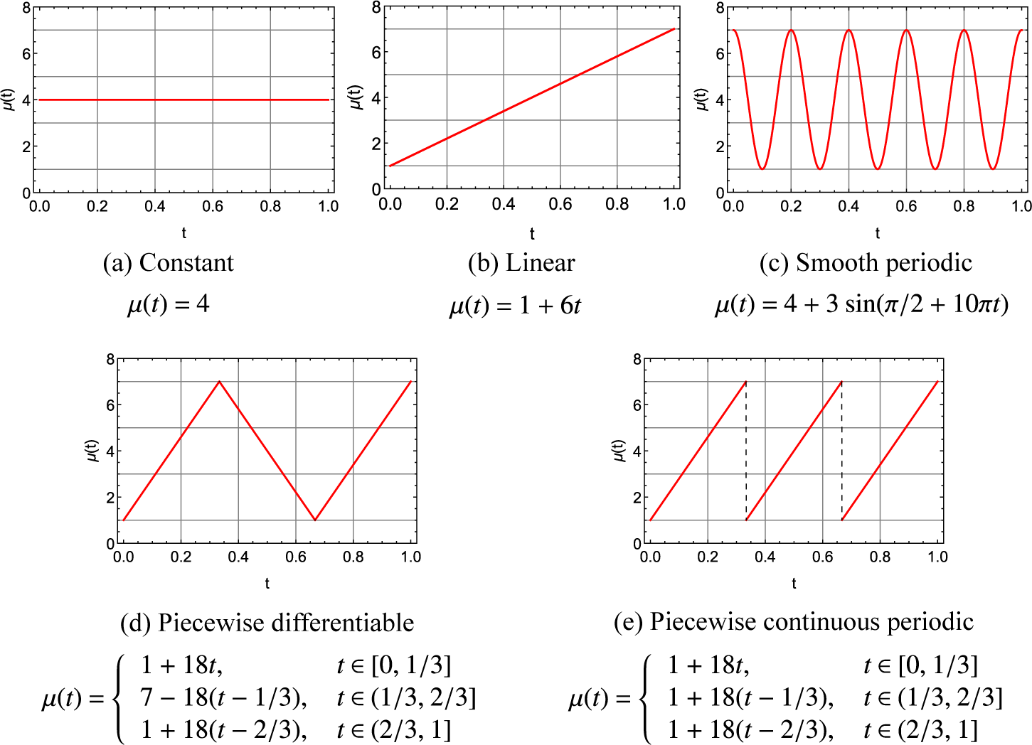
; and five cases of long-run mean functions (constant, linear, smooth periodic, piecewise differentiable and piecewise continuous periodic). The graphs and descriptions of these long-run mean functions
 $\mu :[0,1]\rightarrow \mathbb {R}$
are displayed in Figure 1.
Five cases of long-run mean functions.

3.1. Comparisons with Monte Carlo simulations and Black–Scholes-type formula
To verify the results from our analytical formula, we compare them with the standard benchmark approaches such as Monte Carlo simulations and the Black–Scholes-type formula, since they are quite accurate and simple to perform.
In our comparisons, we compute call and put option prices (1.2) on the underlying asset prices S at the initial time
 $t=0$
,
 $$ \begin{align} v(S,0;\phi) = e^{-rT} \mathbb{E}^{\mathbb{Q}} [ (\phi K-\phi S_T)^+|S_0=S], \end{align} $$
by varying the asset spot price S with the fixed initial time
 $t=0$
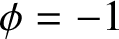
, where
 $\phi =-1$
for call options and
 $\phi =1$
for put options. The other parameters are the risk-free interest rate
 $r = 0.05$
and speed of reversion
 $\kappa = 0.05$
.
3.1.1. Monte Carlo (MC) simulations
Our MC simulations for computing (3.1) employ the simple Euler–Maruyama discretization based on a simple simulation of the mean-reverting process following (1.1), namely,
 $$ \begin{align*} S_{t_i}=S_{t_{i-1}}+\kappa(\mu(t_{i-1})-\ln S_{t_{i-1}})S_{t_{i-1}}\,\Delta t+\sigma S_{t_{i-1}}\sqrt{\Delta t}\, Z_{t_i}, \end{align*} $$
where
 $Z_t$
is a standard normal random variable. We generate sample paths of
 $S_t$
on
 $[0,T]$
, using the time-step
 $\Delta t=0.01$
with 100 000 sample paths.
3.1.2. Black–Scholes-type (BS-type) formula
Suppose that at the initial time t, the initial asset price
 $S_t=S$
. To compute the option value (1.2), one can directly use the definition of expectation with the PDF of the asset log-price at time T,
 $X_T=\ln S_T$
. From (1.3),
 $X_T$
can be represented by
 $$ \begin{align*} X_T =& (\ln S) e^{-\kappa (T-t)} +\frac{\sigma^2}{2\kappa} ( e^{-\kappa (T-t)} -1 ) + \kappa e^{-\kappa T} \int_{t}^{T} \mu(u) e^{\kappa u} \, d u + \sigma e^{-\kappa T} \int_{t}^{T} e^{\kappa u} \, d W_u, \end{align*} $$
which is normally distributed with mean
 $$ \begin{align} m(T)= (\ln S) e^{-\kappa (T-t)} +\frac{\sigma^2}{2\kappa}( e^{-\kappa (T-t)} -1 ) + \kappa e^{-\kappa T} \int_{t}^{T} \mu(u) e^{\kappa u} \, d u , \end{align} $$
variance
 $$ \begin{align} g(T)= \sigma^2 e^{-2\kappa T} \int_{t}^{T} e^{2 \kappa u} \, d u = \dfrac{\sigma^2}{2\kappa} (1-e^{-2\kappa (T-t)}) , \end{align} $$
and PDF
 $$ \begin{align} f_{X}(x) = \frac{1}{\sqrt{2\pi g(T)}}\, \exp\bigg\{-\frac{(x-m(T))^2}{2 g(T) }\bigg\}. \end{align} $$
Using (3.4), the option value (1.2) can be computed by
 $$ \begin{align} v(S,t;\phi)=e^{-r(T-t)} \int_{-\infty}^{\infty} (\phi K-\phi e^x )^+ f_{X}(x) \, d x. \end{align} $$
Note that, to use the formula (3.5) directly, one needs to evaluate the improper integral.
For further simplification, the improper integral (3.5) is derived to get a closed-form formula similar to the Black–Scholes formula for stocks by using the PDF of the asset log-price and the property of normal distribution. The Black–Scholes-type formula is stated as follows.
Theorem 3.1. The value of the European option (1.2) can be represented by
 $$ \begin{align} {v}(S,t;\phi) = \phi K e^{-r(T-t)} \mathcal{N}[ \phi d_1 ] -\phi e^{-r(T-t)+m(T)+g(T)/2} \mathcal{N}[ \phi d_2 ], \end{align} $$
where
 $m(T)$
,
 $ g(T)$
are defined as in (3.2)–(3.3) respectively, and
 $$ \begin{align*}d_1=\dfrac{\ln K -m(T)}{\sqrt{g(T)}},\quad d_2 = d_1 -\sqrt{g(T)}.\end{align*} $$
Proof. From (3.5), note that
 $$ \begin{align} v(S,t;\phi) &= e^{-r(T-t)} \cdot \phi \lim_{n\rightarrow -\infty} \int_{\phi n}^{\ln K} (\phi K-\phi e^x ) f_{X}(x) \, d x \notag\\ &= e^{-r(T-t)} \bigg( K \lim_{n\rightarrow -\infty} \int_{\phi n}^{\ln K} f_{X}(x) \, d x - \lim_{n\rightarrow -\infty} \int_{\phi n}^{\ln K} e^x f_{X}(x) \, d x \bigg). \end{align} $$
Since
 $X_T$
is normally distributed with mean
 $m(T)$
and variance
 $g(T)$
, we have that
 $Z=(X_T -m(T))/(\sqrt {g(T)}$
is the standard normal random variable. Also, since
 $f_{X}(x)$
is the PDF of
 $X_T$
,
 $$ \begin{align} \lim_{n\rightarrow -\infty} \int_{\phi n}^{\ln K} f_{X}(x) \, d x &= \phi\, \mathbb{Q} ( \phi X_T \leq \phi \ln K ) \notag\\ &= \phi\, \mathbb{Q} \bigg( \phi Z \leq \phi \dfrac{\ln K -m(T)}{\sqrt{g(T)}} \bigg) \notag\\ &= \phi\, \mathbb{Q} \bigg( Z \leq \phi \dfrac{\ln K -m(T)}{\sqrt{g(T)}} \bigg) \notag\\ &= \phi \mathcal{N}[ \phi d_1 ], \end{align} $$
where the third equality is obtained from the normal distribution property
 $$ \begin{align*} \mathbb {Q} ( Z \geq x ) = \mathbb {Q} ( Z \leq -x ). \end{align*} $$
Let
 $$ \begin{align*}f_Y(x)=\frac{1}{\sqrt{2\pi g(T)}}\, \exp\bigg\{-\frac{(x-m(T)-g(T))^2}{2 g(T) }\bigg\}\end{align*} $$
be the PDF of a normal random variable with mean
 $m(T)+g(T)$
and variance
 $g(T)$
. By using (3.4), we obtain
 $$ \begin{align} \lim_{n\rightarrow -\infty} \int_{\phi n}^{\ln K} e^x f_{X}(x) \, d x &= e^{m(T)+g(T)/2} \lim_{n\rightarrow -\infty} \int_{\phi n}^{\ln K} \frac{1}{\sqrt{2\pi g(T)}}\, e^{-[(x-m(T)-g(T))^2]/2 g(T) }\, d x \notag\\ &= e^{m(T)+g(T)/2} \lim_{n\rightarrow -\infty} \int_{\phi n}^{\ln K} f_Y(x) \, d x \notag\\ &= \phi e^{m(T)+g(T)/2} \mathcal{N}[ \phi d_2 ], \end{align} $$
where the last equality is obtained by an argument similar to (3.8). Substituting (3.8)–(3.9) into (3.7), the result is obtained.
3.1.3. Notation and comparison results
Let
 $$ \begin{align*} C(S)=v(S,0;-1),\quad P(S)=v(S,0;1) \end{align*} $$
denote call and put option prices computed from our analytical formula (2.5), respectively, and
 $$ \begin{align*} C_{\mathrm{MC}}(S),\ P_{\mathrm{MC}}(S) \text{ and } C_{\mathrm{BS}}(S),\ P_{\mathrm{BS}}(S) \end{align*} $$
denote call and put option prices obtained by MC simulations and BS-type formula (3.6), respectively.
In our numerical tests, we compute the values of
 $C(S)$
,
 $ P(S)$
,
 $C_{\mathrm {MC}}(S)$
,
 $P_{\mathrm {MC}}(S)$
,
 $C_{\mathrm {BS}}(S)$
,
 $P_{\mathrm {BS}}(S)$
, by using various underlying asset spot prices
 ${S\in D_S=\{30,32,\ldots ,48\}}$
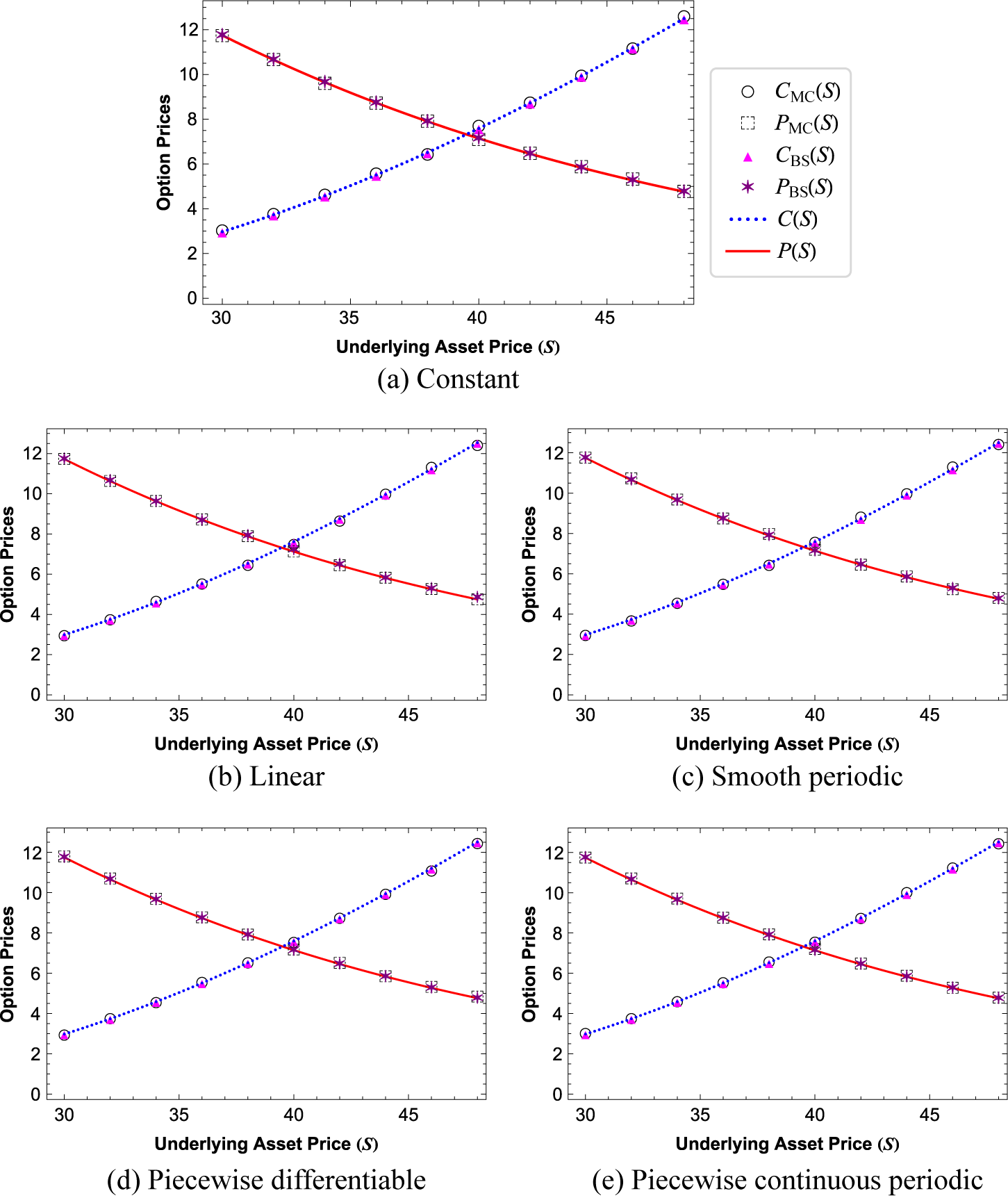
. The option prices obtained from our analytical formula, MC simulations, and BS-type formula are compared based on the five cases of long-run mean functions to illustrate the accuracy of the formula (2.5). The displays of the five comparison results are shown in Figure 2.
Five comparison results of call and put option prices obtained from our formula, MC simulations and the BS-type formula, corresponding to the five cases of long-run mean functions.

3.1.4. Accuracy
According to the comparison results shown in Figure 2, the level of accuracy of the results from formula (2.5) under the five cases of long-run mean functions is demonstrated by the average absolute differences with BS-type and the average percentage errors with MC simulations.
Define the average absolute difference and the average percentage error by
 $$ \begin{align*} \skew6\bar{d}_{\mathrm{BS}}=\bigg( \sum_{S\in D_S} d(S) \bigg)/ |D_S| \quad\text{and}\quad \bar{\epsilon}_{\mathrm{MC}}=\bigg( \sum_{S\in D_S} \epsilon(S) \bigg)/ |D_S|, \end{align*} $$
respectively, where
 $$ \begin{align*} d(S)=| a(S)-x(S) | \quad\text{and}\quad \epsilon(S)=\bigg| \frac{a(S)-y(S)}{a(S)}\bigg|\times 100\%, \end{align*} $$
with
 $a(S)$
representing call/put option value from our formula and
 $x(S)$
,
 $y(S)$
representing call/put option values from BS-type formula and from MC simulations, respectively.
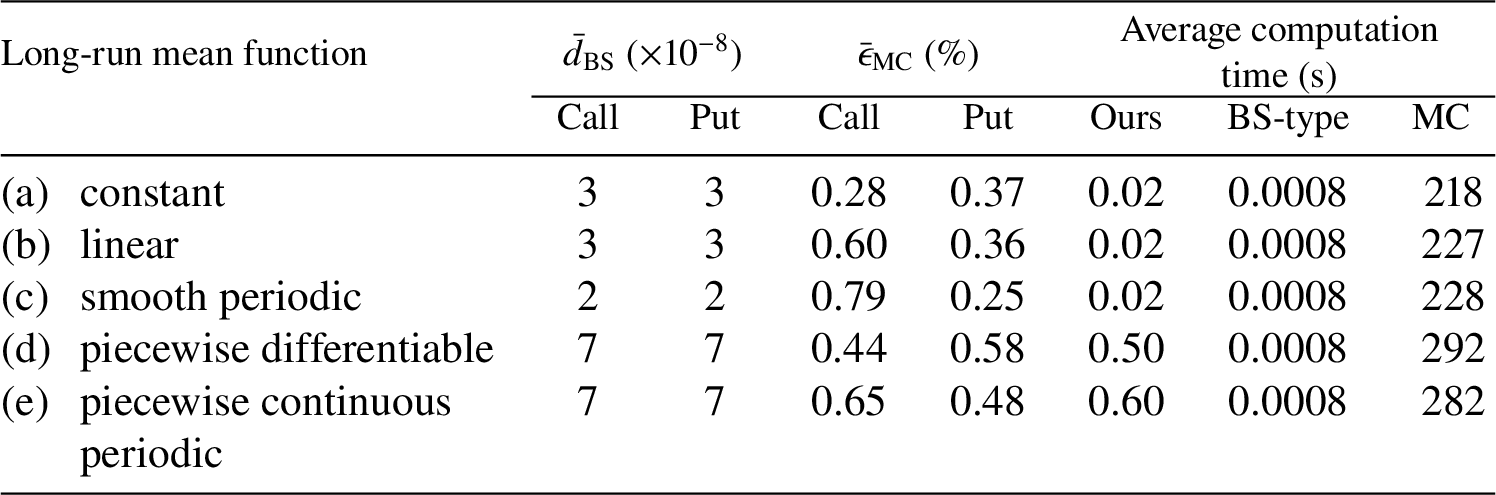
The average absolute differences, the average percentage errors, and the average computation times for each approach corresponding to each long-run mean function are demonstrated in Table 1.
Average absolute differences
 $(\skew6\bar{d}_{\mathrm {BS}})$
and average percentage errors
 $(\bar {\epsilon }_{\mathrm {MC}})$
when comparing the results obtained from our formula with those from the BS-type formula and MC simulations, respectively, and the average computation times for each approach.

Table 1 shows that the results of call and put option values from our formula (2.5) are accurate as compared to the BS-type formula (3.6) with average absolute differences less than
 $10^{-7}$
, and to MC simulations with average percentage errors less than 0.8% for all five cases of long-run mean functions. This fact verifies the validity of the formula (2.5).
Based on the average computation times, Table 1 confirms that the analytical formula (2.5) and the BS-type formula are much more efficient than MC simulations as expected, where the BS-type formula is clearly faster than our formula.
In the next subsection we describe the behaviours of option values as functions of underlying asset price S and initial time t corresponding to various different long-run mean functions.
3.2. Option price behaviour examples and discussion
In this subsection we demonstrate the results of European option values based on the computation of our analytical formula (2.5).
The following examples illustrate behaviours of both European put and call option values
 $v(S,t;\phi )$
on a mean-reverting asset spot price
 $S\in [0,60]$
at time
 $t\in [0,T]$
corresponding to the five long-run mean functions with parameters
 $r = 0.1$
and
 $\kappa = 0.5$
.
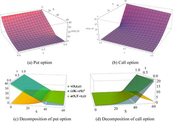
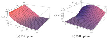
Example 3.2 We consider the constant long-run mean function shown in Figure 1(a). In this case, the underlying asset spot prices do not exhibit seasonality, and follow the one-factor Schwartz model [Reference Schwartz21] used to represent oil and copper prices in commodity markets. The values of put and call options obtained from the analytical formula (2.5) are shown in Figures 3(a) and 3(b), respectively.
Option values for constant
 $\mu (t) = 4$
.

Both figures show that as time t gets closer to the expiration date T, the option value gets closer to the terminal condition
 $v(S,T;\phi ) = (\phi K-\phi S)^+$
as expected with continuous smooth curves in both directions except on the expiration date. Furthermore, when the time t changes and the asset spot price S is fixed, we see that most option values change linearly.
Figures 3(c) and 3(d) illustrate the combination of the option prices
 $v(S,t;\phi )$
, the initial payoff
 $(\phi K-\phi S)^+$
, and the integral term
 $\widetilde {u}(S,T-t;\phi )$
functions for put and call options in Theorem 2.2, respectively. The decomposition of the graph of option price into the others is clearly seen for both options.
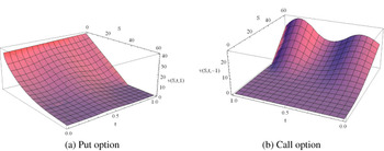
Example 3.3 We consider the case of the linear long-run mean function shown in Figure 1(b), where the spot prices of the underlying asset normally have linear trend without seasonality. The option values obtained from the analytical formula are shown in Figure 4.
Option values for linear
 $\mu (t) = 1 +6 t$
.

Similarly to Example 3.2, as time t gets closer to the expiration date T, the option value gets closer to the terminal condition
 $v(S,T;\phi ) = (\phi K-\phi S)^+$
as expected. However, the figures show quadratic trends when the time t changes and the asset spot price S is fixed. Surprisingly, the call option has the highest value not at the expiration date but around the midpoint of the lifetime of option.
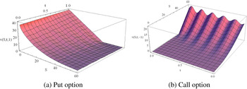
Example 3.4 We consider the smooth periodic long-run mean function shown in Figure 1(c) for the spot price of a seasonal underlying asset. This behaviour of assets is usually seen on most of the agricultural commodities, livestock, energy, and manufactured metal. The option values corresponding to this case are demonstrated in Figure 5.
Option values for smooth periodic
 $\mu (t) = 4+3\sin (\pi /2+10\pi t)$
.

The figures show that the terminal condition
 $v(S,T;\phi ) = (\phi K-\phi S)^+$
holds as in the previous examples. In addition, there are many smooth oscillations on both option values as the time changes with fixed spot price, but the call has stronger oscillations than the put.
Example 3.5 In this example we consider the asset with long-run mean described by the piecewise differentiable function shown in Figure 1(d). The option values obtained from the analytical formula are shown in Figure 6.
Option values for piecewise differentiable
 $ \mu (t) = \left\{\begin {array}{@{}ll} 1+18 t, & t\in [0,1/3], \\ 7-18 (t-1/3), & t\in (1/3,2/3],\\ 1+18 (t-2/3), & t\in (2/3,1]. \end {array}\right.$

Both options show that the terminal condition
 $v(S,T;\phi ) = (\phi K-\phi S)^+$
holds as in the previous examples, with smooth curves even though its long-run mean function is not. The behaviour of the values is similar to those in Example 3.4; there are a few smooth oscillations as the time changes with fixed spot price, and the call has stronger oscillations.
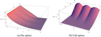
Example 3.6 In this case, we consider the model for assets with seasonality described by a piecewise continuous periodic long-run mean function shown in Figure 1(e), where the spot price changes rapidly when it reaches the high peak. The option values corresponding to this case are demonstrated in Figure 7.
Option values for piecewise continuous periodic
 $ \mu (t) = \left\{\begin {array}{@{}ll} 1+18 t, & t\in [0,1/3], \\ 1+18 (t-1/3), & t\in (1/3,2/3],\\ 1+18 (t-2/3), & t\in (2/3,1]. \end {array}\right.$

Similarly to all previous examples, the results satisfy the terminal condition
 $v(S,T;\phi ) = (\phi K-\phi S)^+$
as expected. Both option values are still continuous and smooth even though their long-run mean function is piecewise continuous. In addition, there are some large smooth waves when the time changes, which are shallower for the put option. There are also some lines between the waves that are changing level rapidly corresponding to the behaviour of jumps on the long-run mean function.
In this subsection Examples 3.2–3.6 demonstrate that both European put and call option values obtained from the analytical formula (2.5) satisfy the terminal condition (1.5) as expected with continuous smooth curves, even though the corresponding long-run mean functions are not continuous or smooth in the domain. In addition, the long-run mean functions provided show strong effects in both options such as linear, quadratic, and oscillation behaviours as the time changes with fixed spot price, in the sense that when the type of the long-run mean function has changed, but the calls are more strongly impacted than the puts. This suggests that the analytical formula can be applied for any kind of mean-reverting assets with integrable long-run mean functions describing both seasonal and nonseasonal behaviours. In addition, Example 3.2 illustrates the decompositions of option prices between the initial payoff term and the integral term from formula (2.5).
4. Conclusion
In this paper, we derive an integral representation formula for pricing the European options on the underlying asset such as commodities whose spot prices follow a mean-reverting model with time-dependent long-run mean. Based on the PDE approach with Fourier transform, the analytical formula together with the put–call parity are presented differently from the traditional Black–Scholes formula. The obtained formula is composed of two terms, the payoff at the initial time and the time-integral over the lifetime driven by the long-run mean function which is only required to be integrable. This implies that the formula can be applied for assets with seasonality described by not only continuous but also discontinuous long-run mean functions. The accuracy of the formula has been verified by comparing with Monte Carlo simulations and a Black–Scholes-type formula under various kinds of long-run mean functions. Moreover, some examples of the European option prices based on our formula are illustrated in order to analyse the behaviours of the option prices corresponding to these long-run mean functions.
Acknowledgements
The first and the second authors gratefully acknowledge financial support from the 90th Anniversary of Chulalongkorn University Scholarship, and the third author gratefully acknowledges financial support from Walailak University under grant no. WU63250. The authors thank an anonymous referee for the suggestion of the Black–Scholes-type formula (3.6). The constructive suggestions from the anonymous referees have substantially improved the readability and representation of the paper. Any remaining errors are our own responsibility.