

INTRODUCTION
Many algorithms exist for determining the relationships between sets of environmental variables (the predictor variables) and the distribution and/or abundance of a pest, a vector tick or insect, the incidence or prevalence of a disease, or the occurrence of a species of conservation interest (the predicted variable). A model capturing these relationships can be applied to the full spatial extent of the predictor variables to produce a ‘risk map’ of the species in question at the present time (Elith et al. Reference Elith, Graham, Anderson, Dudik, Ferrier, Guisan, Hijmans, Huettmann, Leathwick, Lehmann, Li, Lohmann, Loiselle, Manion, Moritz, Nakamura, Nakazawa, Overton, Townsend Peterson, Phillips, Richardson, Scachetti-Pereira, Schapire, Soberon, Williams, Wisz and Zimmermann2006). Because our changing world is likely to bring about significant changes in species’ distributions in the future, models increasingly are being used with future climate scenarios to predict future distributions and to estimate how rapidly species will need to move across the landscape if they are to survive with their current climate sensitivities (Elith et al. Reference Elith, Kearney and Phillips2010; Austin and Van Niel, Reference Austin and Van Niel2011).
The first section of this article shows how these traditional modelling approaches sit on a continuum between statistical and biological approaches. Many of these approaches, despite their names and applications, are in fact aspatial because they do not take into account the conditions in the neighbourhood of each spatial unit as a prediction is made for it (i.e. an ‘assumption of independence’).
The article then introduces the technique of kriging, derived from the field of geostatistics. Whilst there are other geostatistical approaches to the problems addressed here (Hoeting et al. Reference Hoeting, Davis, Merton and Thompson2006), some of them producing more accurate results than kriging in certain situations (Kravchenko, Reference Kravchenko2003), kriging techniques are based upon a considerable body of previous research in other areas, especially mining, that have only recently spread into the field of biology. Kriging is a truly spatial technique that has certain advantages in making predictions of species' and diseases' presence and absence when the data are incomplete. Importantly, geostatistical techniques (termed ‘classical’ (Matheron, Reference Matheron1963), ‘model based’ (Diggle et al. Reference Diggle, Tawn and Moyeed1998) or ‘modern’ (Christakos, Reference Christakos2000)) and recent Bayesian spatial regression models (Chiogna and Gaetan, Reference Chiogna and Gaetan2010), unlike many other spatial techniques (such as cluster identification), provide estimates of the variability of their predictions and the spatial scale of the phenomena under study (Wagner and Fortin, Reference Wagner and Fortin2005; Bellier et al. Reference Bellier, Monestiez, Durbec and Candau2007). The main advantages in using a Bayesian framework as opposed to the classical geostatistical methods are: (1) it is flexible in the model types that are allowed (e.g. spatial general linear models) (Kelsall and Wakefield, Reference Kelsall and Wakefield2002; Hampton et al. Reference Hampton, Serre, Gesink, Pilcher and Miller2011), (2) the underlying spatial process need not be Gaussian; (3) estimation of the spatial correlation parameters is an automatic part of the analysis; and (4) it easily allows for heteroscedasticity of the data (common in disease rates; for example Berke (Reference Berke2004)). These advantages, however, come at the cost of a complex likelihood function that requires a large number of parameters to be estimated, and restricts the choice of priors. Hence classical kriging has to date found widespread use in epidemiology (Carrat and Valleron, Reference Carrat and Valleron1992; Oliver et al. Reference Oliver, Muir, Webster, Parkes, Cameron, Stevens and Mann1992; Liu et al. Reference Liu, Jiang, Liu, Wang, Li, Yuan, Wang and Xue2011).
Secondary environmental data may be used to increase the accuracy of kriged predictions through cokriging (Journel and Huijbregts, Reference Journel and Huijbregts1978; Perez et al. Reference Perez, Thurmond and Carpenter2006; Li and Heap, Reference Li and Heap2011), but only if they are more numerous than the primary data. Secondary data need have no obvious biological significance, and cokriging cannot therefore be used either to identify biologically important variables or to select from a suite of variables a subset that best (of all possible subsets) describes a species’ distribution. However, the choice of secondary data is likely to influence both the optimisation of the fixed term (i.e. the trend) and the autocorrelation parameters (Lennon, Reference Lennon2000; Crase et al. Reference Crase, Liedloff and Wintle2012; De Iaco et al. Reference De Iaco, Maggio, Palma and Posa2012). Application of kriging techniques is here illustrated using a unique set of disease outbreak data, that of bluetongue virus serotype 8 in northwest Europe. Finally, the article includes some warnings. Use of spatial covariates can lead to worse predictions when important kriging assumptions are violated.
None of the ideas presented in this article is new, although the way they are presented will, we hope, make them accessible to biologists who have so far mostly ignored the spatial context in the models they have used. For an excellent overview of spatial analysis the reader is referred to Fortin and Dale (Reference Fortin and Dale2005). Rossi et al. (Reference Rossi, Mulla, Journel and Franz1992) provide examples of further application to ecological studies, Franklin and Miller (Reference Franklin and Miller2009) specifically address species' distributions and Dormann et al. (Reference Dormann, McPherson, Araujo, Bivand, Bolliger, Carl, Davies, Hirzel, Jetz, Kissling, Kuhn, Ohlemuller, Peres-Neto, Reineking, Schroder, Schurr and Wilson2007) review methods accounting for spatial autocorrelation in species' distribution data. More advanced geostatistical techniques are covered by Goovaerts (Reference Goovaerts1997) and Webster and Oliver (Reference Webster and Oliver2007), whilst Lai et al. (Reference Lai, So and Chan2009) deal specifically with epidemiological studies.
Geostatistical calculations are today made easy by the R software suite (http://www.R-project.org/), in particular the packages RandomFields (Schlather, Reference Schlather2001), fields (Furrer et al. Reference Furrer, Nychka and Sain2012), gstat (Pebesma, Reference Pebesma2004) and geoR (Ribeiro and Diggle, Reference Ribeiro and Diggle2001).
DISEASE AND ENVIRONMENTAL DATA
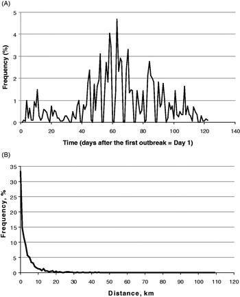
Bluetongue (Family Reoviridae) is a viral disease of domestic and wild animals. In the Old World this disease was restricted to tropical and sub-tropical areas, but in 2006 it spread for the first time into temperate NW Europe. The first case of bluetongue in this part of Europe was recorded on August 17th 2006 and further cases were reported up until December 15th in that year. The time-course of these infections is shown in Fig. 1A. By the end of 2006, a total of 2025 infected farms had been recorded, covering an area of approximately 500 (EW direction) by 350 (NS direction) km. Given the veterinary importance and the novelty of this disease in this area we have every reason to believe that essentially all outbreaks were recorded by the monitoring system in each affected country, co-ordinated at the European level by the European Union's European Food Safety Authority (EFSA). Previous publications using this dataset have also assumed it is effectively complete (Gerbier et al. Reference Gerbier, Baldet, Tran, Hendrickx, Guis, Mintiens, Elbers and Staubach2008; Hendrickx et al. Reference Hendrickx, Gilbert, Staubach, Elbers, Mintiens, Gerbier and Ducheyne2008; Mintiens et al. Reference Mintiens, Meroc, Faes, Abrahantes, Hendrickx, Staubach, Gerbier, Elbers, Aerts and De Clercq2008; de Koeijer et al. Reference de Koeijer, Boender, Nodelijk, Staubach, Meroc and Elbers2011). Fig. 1A, however, also strongly suggests a ‘weekend’ effect in reporting. Case numbers drop to near zero at weekends and this is especially noticeable during the period of high case numbers. Hence, whilst the spatial data are probably complete, there may be errors in the reporting dates of the infections. Further details and a statistical analysis of this outbreak are given by Sedda et al. (Reference Sedda, Brown, Purse, Burgin, Gloster and Rogers2012), while a description of the overall epidemic in 2006 and 2007 is given by Wilson and Mellor (Reference Wilson and Mellor2009). For present purposes we only need note that we have a relatively accurate spatial and temporal record of this outbreak; what we lack are records of farms that remained uninfected throughout the outbreak period.
(A) The time course of the BTV-8 outbreak in NW Europe in 2006. This epizootic began on August 17th 2006 (Outbreak Day 1 in the figure) and ended on December 15th (Outbreak Day 122). The figure shows the farms reported as infected on each day, expressed as a percentage of the total of 2025 farms infected during 2006. (B) The frequency distribution of the distances between farms on the day of their infection with BTV-8 in 2006 and the nearest previously infected farms. Frequencies are expressed as percentages of all farms eventually infected in 2006. The modal distance between farms is < = 1 km.

Environmental data used in this study came from the MODIS sensor on NASA's Terra and Aqua satellites (Justice et al. Reference Justice, Townshend, Vermote, Sohlberg, Descloitres, Roy, Hall, Salomonson, Riggs, Huete, Didan, Miura, Wan, Strahler, Schaaf, Myneni, Running, Glassy, Nemani, El Saleous and Wolfe2000). Data for the years 2001 to 2008 inclusive were temporal Fourier processed (Rogers and Williams, Reference Rogers, Williams, Edwards, May and Webb1994; Rogers, Reference Rogers, Hay, Randolph and Rogers2000) to produce sets of orthogonal data that capture important features of the annual seasonality of the local environment; the mean, the annual, bi-annual and tri-annual amplitudes and phases, the maxima, minima and variances of the middle infra-red (MIR) daytime Land Surface Temperature (dLST), night-time LST (nLST) and the Normalised Difference Vegetation Index (NDVI) signals (Scharlemann et al. Reference Scharlemann, Benz, Hay, Purse, Tatem, Wint and Rogers2008).
TRADITIONAL MODELLING APPROACHES
A variety of assumptions is made in traditional species' distribution models about the statistical distribution of the predictor variables, their relationship with the predicted variable and the statistical distribution of the error term. As pointed out elsewhere, some of these assumptions follow on from a body of more general ecological theory arising from the work of Robert Macarthur and his co-workers (Macarthur, Reference Macarthur1972; Rogers, Reference Rogers2006), but many distribution models achieve impressive predictive accuracies using quite different assumptions and select and treat predictor variables in quite different ways. This may be due to one or more of the following factors: (1) Models are in fact more similar than first appearances might suggest (Austin, Reference Austin2007). This seems unlikely given the very different nature of the models. (2) One or more predictor variables in one model may be substituted in different models by others which have collectively the same statistical power. Neither set of variables might be particularly important biologically, although it is likely that at least some among them probably are. This raises a two-fold problem arising from the multi-collinearity of predictor variables, statistical and biological. Statisticians must decide which of the collection of multi-collinear variables should be used to make parsimonious models, whilst biologists must decide which of the variables is most likely to be acting on biological processes (Graham, Reference Graham2003). (3) Models may in fact be describing an inadequate training dataset (the set of observed points) rather than a species' actual distribution. Describing a set of data is easier than capturing statistically the manifold processes that underlie any species' full distribution. Over-fitting is an especial danger here, when complex models are fitted to small datasets. (4) Different sorts of models are treating species' spatial distributions in very different ways; effectively as different ‘problems’ rather than as a single one. For example, some approaches tackle the entire dataset as a single unit (a single-piece jigsaw puzzle) whilst others effectively break up a species' distribution into many different jigsaw pieces; included here are neural network models (Pearson et al. Reference Pearson, Dawson, Berry and Harrison2002), various regression trees (Breiman, Reference Breiman1984) or random forest models (Breiman, Reference Breiman2001) and their bootstrap implementations (Elith et al. Reference Elith, Leathwick and Hastie2008). Each jigsaw piece is then described separately and the jigsaw puzzle is re-constituted using the known original locations of the pieces, not the overall pattern (the functional relationships) that the correctly re-assembled pieces might reveal. Various generalised additive models, GAMs (Hastie and Tibshirani, Reference Hastie and Tibshirani1986), straddle these two approaches (Guisan et al. Reference Guisan, Edwards and Hastie2002); very flexible functions are fitted to the training set data plotted against the predictor variables across the entire area to be predicted. The shape of the GAM functions (often taking complex forms) is determined by the predictor variables sampled at the locations of the training set data, but not by their geographical location. Increasing levels of smoothing, applied to the predictors of the GAM functions, is analogous to moving from the multiple jigsaw piece puzzle (little smoothing) to the single jigsaw piece puzzle (considerable smoothing).
There is a spectrum of modelling approaches, from purely statistical or data driven to purely biological, the latter based on the functional relationships between biological parameters and environmental and other variables. Each of the above factors (1–4) is more important in data-driven modelling approaches (e.g. neural network and tree-based models) where the results are very data dependent. Adding or removing data points can affect the resulting models considerably, and therefore model predictions.
Other modelling approaches assume a pre-defined response function of a species to a single (or set) of environmental variable(s). In general, these response functions are chosen from a limited set of prescribed types, easily described mathematically. In such models, the training set is used to derive parameter values without re-defining the functional relationship between the predictor and predicted variables, which remains unchanged. Logistic and other regression methods fall into this category, as do various forms of discriminant analysis (Rogers, Reference Rogers2006).
A third modelling approach begins in the realm of biology and the known or assumed relationship between a species and a variety of environmental variables. For example, a species' tolerance of low, medium and high temperatures can be coded into a response function unique to that species and irrespective of any information that may be contained within, or derived from, the training set. Various fuzzy logic and climate-based models, for example CLIMEX, (Sutherst and Maywald, Reference Sutherst and Maywald1985), fall into this category. These are the only models in which model derivation could be entirely independent of any field data from the species' geographical distribution. The occurrence of the species in places predicted for it, and its absence elsewhere, would be a strong test of this sort of model's predictive abilities. In practice, however, such models are very often developed iteratively using the training set data to ‘fine tune’ an initial version which is often very inaccurate. The training set data then cease to be independent of model predictions and no independent statistical test of these predictions can be carried out.
General problems of applying species' distribution models, a discussion of some of the important assumptions involved (for example, whether what is being fitted is the fundamental, realised or potential niche) and some of the challenges presented by spatial dependence, population mobility and environmental change are discussed by Guisan and Thuiller (Reference Guisan and Thuiller2005).
The spatial context of disease data
Despite the many differences between these traditional modelling approaches, they all share something in common; their usual implementation does not involve spatial statistics of any sort. That is to say, with very few exceptions the models are developed relating the presence or absence of a species at any particular point to the environmental and other conditions at the same point. Neither the presence nor absence of the species, nor the environmental conditions elsewhere is used as information that may determine the likelihood of occurrence of the species at the point in question. Yet it seems highly likely that conditions in nearby areas can and do influence the presence or absence of a species, either as a result of processes intrinsic to the population concerned (for example the migration of individuals from high density patches) or extrinsic to them (for example favourable environmental conditions that increase the survival of the species throughout areas much larger than the sampled points).
Using information from nearby areas to make predictions of species' presence and absence takes modelling into the realm of true spatial statistics, a rather large field which itself has many different modelling approaches. Some sorts of spatial analysis simply identify clusters of disease cases (Diggle, Reference Diggle2003), a first step in identifying the likely causes of the clusters, for example the presence of disease vectors, or of environmental contaminants that may cause chronic diseases (see Souris and Bichaud (Reference Souris and Bichaud2011) for new developments in this field). These methods are purely descriptive; it is generally not possible to use them to make predictions of the occurrence of cases of the same disease in un-sampled areas, or into the future.
Other spatial techniques, derived from the fields of geology and mining, are designed not only to analyse present patterns but also to make prediction of the patterns in other places, and even times (estimation). These ‘geostatistical’ techniques are increasingly being used in biological applications and this article provides a primer of them for biologists interested in true spatial mapping of vectors, diseases or indeed any biological system with a spatial component. Geostatistics, a brief history of which is given by Oliver (Reference Oliver, Fischer and Getis2010), allows the values of variables within a certain spatial range of any point to affect the estimate of the value of the predicted variable at that point, thereby improving the precision of the estimate (Isaaks and Srivastava, Reference Isaaks and Srivastava1989). It achieves the latter by identifying (and using in the estimation procedure) that component of the error variance of a non-spatial model which is attributable to the spatial structure that occurs when things that are closer together are more similar to each other than things that are farther apart (the “first law of geography” (Tobler, Reference Tobler1970)).
Approaching species' distribution modelling from the point of view of biologists, we seek to answer the following questions: (1) How may geostatistical methods be used to improve predictions of species distributions? (2) What assumptions are being made in the process, and are they always realistic for biological systems? (3) What, if anything, can we learn from the application of these techniques about the biological processes underlying species distributions?
In answering these three questions we are aware of the fact that one particular pattern may be derived from several different processes and one process may give rise to several different patterns. Therefore a technique that only describes pattern is unlikely to tell us anything about process; conversely, one that concentrates on process may predict a variety of patterns. It follows from this that we must be extremely careful in choosing the metric by which we judge goodness of fit of the resulting models, and that we may need to settle for a compromise between a model that is statistically good but biologically poorly founded and one that gives poorer statistics but is more firmly grounded in sensible biology.
DATA ANALYSIS
Experimental and model variograms
Knowledge of the spatial context of any process is useful when the value of a variable at a point is similar to the value of the same variable at nearby points. That this is likely to be the case here is shown by Fig. 1B that records the frequency histogram of distances from each BTV-8 case to the nearest previous case. Fig. 1B suggests strongly that throughout the BTV-8 outbreak in 2006 the occurrence of infections on nearby farms was an important determinant of new infections.
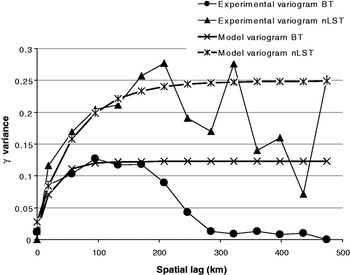
Evidence in support of this idea is shown in Fig. 2 that relates the half mean squared difference (a quantity traditionally called the ‘semivariance’ now no longer favoured and here replaced by ‘γ-variance’, as suggested by Bachmaier and Backes (Reference Bachmaier and Backes2011)) between the BTV-8 status on all pairs of farms on day 40 of the outbreak (by which time 224 farms were infected and 1801 were uninfected) to the distance between them, called the ‘lag’ (a term derived from time series analysis that provides a number of the formulae used in spatial analysis). The raw data plot in Fig. 2 is the value of γ-variance at the ordered lags, and is usually called the ‘experimental’ or ‘empirical’ or ‘sample’ variogram,  $\hat\gamma\, (h)$.
Experimental (i.e. observed) and model variograms of BTV-8 infected farms 40 days after the start of the outbreak in 2006 (lower pair of lines) and experimental and model variograms of mean night-time Land Surface Temperature (upper pair of lines); both sets are from across the entire area eventually infected with BTV-8 in 2006. The nLST data were standardized before analysis and their variograms were re-scaled (divided by 5) to facilitate comparison.

The experimental variograms are usually calculated by Matheron's Method of Moments (Matheron, Reference Matheron1965):
 $$\hat \gamma \left( {h} \right) = \displaystyle{1 \over {2N\left( {h} \right)}}\sum\limits_{i = 1}^{N({ h})} {\left[ {z\left( {{x}_i} \right) - z\left( {{x}_i + h} \right)} \right]^2} $$
Where h is the (lag vector) separation between two locations, N is the number of pairs of data points separated by the lag h, z(x) is the value of the attribute at location x and z(x + h) the value at a location at distance h away from x. In the simplest case of a pure spatial analysis, with little directional variability in the values of $\hat\gamma (h)$, h is the Euclidean distance between two points in a Cartesian system (or the haversine distance in longitude/latitude coordinate form). In other cases, h must be adjusted for directional changes in variance; in the case of full spatio-temporal analyses (not covered here) h has the dimensions of both space and time. Fairly obviously, for a dataset from a limited geographical area the number of paired locations, N, decreases with distance, h (i.e. in the present example there are fewer pairs of distant farms than nearby farms). In the simplest forms of kriging (when variances do not change over space, a condition known as ‘weak stationarity’), the covariance Ĉ(h) depends only on distance, h, as follows:
 $$\hat C\left( {h} \right) = C\left( 0 \right) - \hat \gamma\, (h)$$
where C(0) is the sample variance, calculated using all values of z (Oliver, Reference Oliver, Fischer and Getis2010). Equations 1 and 2 are sample estimates of the (unknown) underlying variogram and variance respectively (Dunn, Reference Dunn1983). Notice that for small h in equation 1, the difference between the two z values is likely to be small, so that ŷ(h) is also small, making the covariance Ĉ(h) in equation 2 similar to the sample variance C(O). ŷ(h) increases, and Ĉ(h) therefore decreases, as h increases.
As is usually the case, the BTV-8 experimental variogram in Fig. 2 first rises quickly with distance, reaching an initial plateau at a lag of 80 to 100 km, indicating that locations which were close to each other had smaller differences between them in terms of their infection status than locations which were farther apart. Thereafter, the experimental variogram normally stays more or less constant at a plateau (because it reaches the value of the sample variance), but in the present case it decreases because all farms at these large distances apart are still uninfected by day 40 (in geostatistics this is called the ‘hole effect’ and is often related to a sampling problem). Alternative ways of displaying the same data involve plotting either the covariances (i.e. equation 2) or the correlation between pairs of farms at the same lags; such graphs are ‘mirror images’ of Fig. 2, being higher at lower lags and decreasing with increasing lags.
Various smoothed functions can be fitted to the data in Fig. 2 to produce a statistical description of how the experimental variogram increases with lag (a ‘model variogram’ or ‘theoretical variogram’). Variogram fitting is a user-controlled procedure in which the experimental variogram is modelled using one (occasionally more) of a limited number of forms called ‘authorized functions’ that have the characteristic that the variance of the random variable cannot be negative or equal to zero (the covariance function must be ‘positive definite’ or the variogram ‘conditionally negative semidefinite’). Examples of authorised functions include exponential, circular spherical, Bessel and Matérn functions, and combinations of these which are also positive definite (Shapiro and Botha, Reference Shapiro and Botha1991). As hinted above, full spatio-temporal models are different in a number of respects from purely spatial models and for them the Dagum function is recommended (Porcu et al. Reference Porcu, Mateu, Zini and Pini2007). Fitting these functions to the observed data involves least squares or weighted least squares methods, maximum likelihood or residual maximum likelihood methods (the latter particularly useful in the case of small sample sizes) (Zimmerman and Stein, Reference Zimmerman, Stein, Gelfand, Diggle, Fuentes and Guttorp2010) or Bayesian methods (Ecker and Gelfand, Reference Ecker and Gelfand1997; Diggle et al. Reference Diggle, Tawn and Moyeed1998). An accurate variogram is essential for kriging to be superior to inverse distance methods (Kravchenko, Reference Kravchenko2003).
The theoretical variogram of BTV-8 is shown in the Fig. 2, obtained by fitting the following K-Bessel function (Gaetan and Guyon, Reference Gaetan and Guyon2010) to the experimental variogram data:
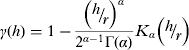 $$\gamma \left( {h} \right) = 1 - \displaystyle{{\left( {{\raise0.7ex\hbox{$h$} \!\mathord{\left/ {\vphantom {h r}}\right.\kern-\nulldelimiterspace} \!\lower0.7ex\hbox{$r$}}} \right)^\alpha} \over {2^{\alpha - 1} \Gamma \left( \alpha \right)}}K_\alpha \left( {{\raise0.7ex\hbox{$h$} \!\mathord{\left/ {\vphantom {h r}}\right.\kern-\nulldelimiterspace} \!\lower0.7ex\hbox{$r$}}} \right)$$
where r is the distance (known as the ‘spatial range’) at which the variogram levels off (at a value of γ-variance known as the ‘sill’), Γ is the gamma function and K is the modified Bessel function of order α (where α is the shape parameter). The spatial range in Fig. 2 is about 100 km.
The variogram drops towards zero at small lags, and should reach zero at a lag of zero. In practice, however, experimental and/or model variograms can have non-zero γ-variances (called the ‘nugget’) at this lag, indicating variability at distances shorter than the lag interval, or some form of error (e.g. measurement error). In the case of the BT data, the nugget is effectively zero (Fig. 2).
Ordinary and Indicator kriging
In the absence of any measure of a variable at a particular point, we may use the model variogram of equation 3 to produce an estimate of it. Let us assume, for example, that we wish to know the level of a disease (y i) at location (i), but that we have no direct measure of it; we have only a series of local observations at different distances from i. Our estimate is derived by a process called ‘ordinary kriging’ (Matheron Reference Matheron1963), using the following equation:
 $$y_i = \sum {w_d y_d + \varepsilon} $$
Where y d is the observed value of y at a location a distance d away from i, w d is the weight for that point and ε is the kriging error.
It is very important to understand the nature of the weights in equation 4, which vary from one location to the next and are not simply dependent upon the distance of a known point from the point being predicted (as they would be in any inverse square measure of action at a distance). Weights are defined for an area around the point i that includes other points at different distances, d, from i. These other, local points, j (j < > i), are also at different distances from each other. Knowing these distances, the fitted model variogram is used to define both (1) the covariance matrix that describes how the presence or absence status of the local points, j, co-vary with distance from each other and (2) the vector of covariances between the single point i and all the j points. The weights are calculated to reconcile the information in these two matrices. That is to say, they effectively answer the question “What weights would we need to apply to the elements in the covariance matrix for the j points, for which we have complete information, to produce the elements in the covariance matrix for point i, for which we know only the location, not the infection status?” Having determined the weights (which in ordinary kriging sum to 1·0), they can then be used in equation 4 to predict y i.
More formally, the weights are obtained by solving the ordinary kriging system equation which is shown for illustration purposes in equation 5, considering only three known points, y 1, y2, and y 3, and one unknown point y i:
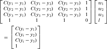 $$\left[ \matrix{C(y_1 - y_1 )\quad C(y_1 - y_2 )\quad C(y_1 - y_3 )\quad 1 \hfill \cr C(y_2 - y_1 )\quad C(y_2 - y_2 )\quad C(y_2 - y_3 )\quad 1 \hfill \cr C(y_3 - y_1 )\quad C(y_3 - y_2 )\quad C(y_3 - y_3 )\quad 1 \hfill \cr \quad 1\quad \quad \quad \quad \quad 1\quad \quad \quad \quad \quad 1\quad \quad \quad \quad 0 \hfill} \right]\;\left[ \matrix{w_1 \hfill \cr w_2 \hfill \cr w_3 \hfill \cr l \hfill} \right]\hskip-20pt\cr\tab = \;\left[ \matrix{C(y_i - y_1 ) \hfill \cr C(y_i - y_2 ) \hfill \cr C(y_i - y_3 ) \hfill \cr 1 \hfill} \right]$$
Where C(…) indicates the covariances from equations 2 and 3, and l is the Lagrange multiplier, use of which minimises the kriging error. Notice that whilst y i itself is unknown in equation 5, the values of C(y i – y1), C(yi – y2) etc. are known from equation 2 because they are determined only by the physical distances between the point y i and y 1, y2, etc. and the theoretical variogram, equation 3, fitted to the experimental variogram of equation 1, where all values are known. Equation 5 is soluble by standard matrix procedures, because there are as many equations as there are unknowns (the weights, w 1, w2, and w 3, and the Lagrange multiplier, l), and it has a unique solution for any particular set of predictor points.
Ordinary kriging produces exact predictions of the observed data points (i.e. the y d in equation 4) because in such cases the weight is 1 for the observed data point and zero for all the other points in the vicinity; hence only the observed data point contributes to its own estimate, and the variance of this estimate is zero. For all other points for which predictions are made, several local points are used to estimate y i, and the weights are calculated to minimize the variance of this estimate, which is always non-zero. One of the important features of geostatistics is that it quantifies the errors of predicted values. The prediction variance (the square root of which is the prediction error) is given by the following equation:
 $$\sigma ^2 ( {y_i} ) = l + \sum\limits_{}^{} {w_d \gamma ( {y_d, y_i} )} $$
where l is the Lagrange multiplier obtained from equation 5 and γ is the theoretical variogram. It is clear that the error depends on the spatial configuration of the local data and not (only) on their absolute value. In this way, geostatistical techniques differ from other deterministic spatial techniques (e.g. cluster identification).
Ordinary kriging is appropriate for many continuous variables with normally distributed errors, but is not directly applicable to discontinuous variables such as binary coded presence/absence or categorical data which are usually non-normally distributed. For such data the alternative ‘indicator kriging’ is often used. The mechanics of applying indicator kriging are similar to those of ordinary kriging. Experimental and model variograms are prepared as before; even though the data points take integer values, the variogram are continuous. The ordinary kriging equations are then applied and produce a continuous prediction in the range of zero to 1·0, which is thresholded to produce a discontinuous output on the basis of the frequency distribution of the observed points (the ‘empirical distribution’, transformed to a conditional cumulative distribution function; Webster and Oliver (Reference Webster and Oliver2007)). Formal details of indicator kriging, and worked examples, are given in Goovaerts (Reference Goovaerts1997). Indicator kriging which, like ordinary kriging, gives exact predictions of the input data, is particularly useful in the fields of pedology and pollution monitoring. A polluting variable can be thresholded at a number of different levels representing different degrees of impact on human or animal health. The covariation of any particular level of a pollutant and the cross variation of different levels of the pollutant may be used in indicator kriging to define areas of different degrees of pollution hazard.
Important kriging assumptions
A very important assumption of many spatial analyses is that of stationarity. There are several types of stationarity in spatial analysis, but most of the models imply a second order stationarity (also called ‘weak stationarity’) that assumes that neither the mean nor the variance (in this case the sill) of the process varies over space (Myers, Reference Myers1989).
Biological data are rarely stationary, and non-stationarity commonly arises in several ways; either the mean value varies spatially (often associated with changing environmental conditions, for example from drier to wetter conditions), or the variogram changes locally (due to finer resolution changes in a disease or species' demographic parameters, or to the environmental conditions affecting these parameters). Finally, spatial variation around each point may have a component of direction, for example along a stream passing through the sampled area, or when a prevalent wind disseminates contaminants from an industrial chimney, a condition called anisotropy (Journel and Huijbregts, Reference Journel and Huijbregts1978). Anisotropy may involve the sill (‘zonal anisotropy’), the range (‘geometric anisotropy’) or both. Non-uniformity across a study area means that indicator and other sorts of kriging cannot be applied directly, and several solutions to this problem have been developed (see Fortin and Dale (Reference Fortin and Dale2005) for a discussion). We will mention briefly one of them. If the mean value of the kriged variable (in the present case the means of presences and absences) varies across the study area, the first step before kriging would be to capture this variation using a linear or non-linear regression type of model, with one or more external variables, or even the geographical location (x, y; longitude or latitude), as the independent predictors. Once formulated, this regression model is used to define a mean surface or ‘trend’, the local values of which are subtracted from the local observations, thus generating a set of values (differences from the local mean) which should no longer show any spatial trends; kriging is then applied to these ‘residuals’ and the results arising from kriging are added back to the local trend surface to produce the output predictions (these variants are implemented in ‘universal kriging’, ‘kriging with trend’, ‘regression kriging’ and ‘kriging with external drift’ methods). Regression kriging is described by Christensen (Reference Christensen2001) and was applied to species’ distribution models by Latimer et al. (Reference Latimer, Wu, Gelfand and Silander2006). Journel and Rossi (Reference Journel and Rossi1989) applied a step-wise constant ordinary kriging method to trending data and showed that in some situations this produces similar results to regression kriging. An alternative to the above is to allow for the trend within a kriging framework, a technique called ‘ordinary moving kriging’.
Needless to say, the occurrence of un-acknowledged variation in a kriged variable's mean or variance may result in the blind application of equations 1 to 5 producing a less accurate prediction than their non-spatial equivalent, which is simply the mean level of disease across the entire area. Thus, simply showing that a set of data requires spatial analysis (for example, by examining a map of deviations of a variable from its mean value) is not itself sufficient to guarantee that a spatial analysis using kriging without trend correction will give a better prediction than a non-spatial one.
If all of the above considerations are resolved satisfactorily, we could use kriging methods to predict the BTV-8 outbreak data for any location i, using all the observations of BTV-8 within a user-definable distance of the location concerned to define the weights, w d. Whilst the spatial range is the obvious limit for this user-definable distance, any value may be chosen, from close to zero up to (generally half of) the maximum distance between any two locations in the dataset. Maximum smoothing of a kriged surface is obtained when all the sample data are used to define the weights.
The origins of kriging
The initial approach to spatial analysis of disease data presented here is informed by a history of spatial statistics derived for non-biological purposes such as mining (Krige, Reference Krige1951). The surface concentrations of particular minerals result from many thousands or millions of years of erosion, leaching and diffusion and have presumably reached some sort of near-equilibrium in which the amount of variation over short distances is limited. Biological systems change on a much shorter temporal and finer spatial scale than do many inorganic mineral concentrations, so the application of equations from this field to biology should be undertaken with care. We persevere, however, because biological systems also involve concentration effects (e.g. breeding sites) and diffusion effects (e.g. migration), obvious analogues of the processes determining mineral concentrations. Tools from one field may be useful in other fields with analogous processes.
Application of kriging
Kriging and its derivatives can be incorporated into a wide range of models, from simple regressions to GAMs, turning them from aspatial models into spatial ones. In the present case we have all the data for this BTV-8 outbreak so we do not need kriging to estimate them. But we could also use kriging to predict farms that are dropped from the calculation of the experimental variogram, to investigate how accurately kriging estimates ‘missing data’ (an exercise called ‘cross validation’). Or, more usually, we could use kriging on an incomplete data set to predict the disease at a series of points of interest for which we have no direct disease information (‘estimation’).
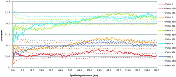
Variograms may change not only in space, but also through time. The variograms of the BTV-8 data for 20-day intervals (P1 to P5) during the 2006 outbreak are shown in Fig. 3. The sill variances and the ranges are greatest for periods 3 and 4, in the middle of the outbreak. Both are lower for the first period and for the last period, period 5 in Fig. 3, by which time virtually all the farms are infected. Whilst some of the features of Fig. 3 are artefacts of this particular dataset (which includes only farms that are eventually infected by the end of 2006), it also suggests strongly that temporal as well as spatial changes may introduce variation in covariances of disease systems.
Experimental variograms of the 2006 BTV-8 data for five sequential periods of 20 days each, colour coded red, orange, green, blue and purple respectively (solid lines). The dotted lines show the upper and lower limits of the variogram permutations (e.g. ‘Period 1SU’ and ‘Period 1SL’ for the limits in Period 1) when the infection statuses are randomly re-arranged across the same farm locations. Such re-arrangement destroys all signs of spatial clustering of the outbreak data.

Are the differences between the different graphs in Fig. 3 significant? There are no standard statistical tests for variograms, and significance is therefore often determined by permuting the data (or sometimes the model parameters) in either space or time, carrying out the same sorts of analysis and finding out how often is observed a result as extreme as the one obtained. Fig. 3 also includes (as dotted lines) the envelopes derived from 500 such re-arrangements of each dataset. Clearly any spatial structure in the data should be eliminated by randomly re-arranging the data, and this appears to be the case here. Temporal variation, however, remains, with three groups (P1; P2 and P5; P3 and P4) showing different sill variances of their variograms. Taking Period 4 as an example, the permuted γ-variances are greater than the observed γ-variances at distances up to about 100 km and about the same as observed, or slightly less, at greater distances. The distance at which observed and permuted data first have about equal γ-variances is approximately the range at this time, as might be expected. Similar results can be seen for the other periods. Permuting the data in this way highlights the fact that the kriging equations are designed to explore the random errors of spatial data with a constant mean value, when those errors are spatially structured. Re-arranging the data does not affect the mean value, only the spatial arrangement of the errors, which is destroyed in the process of re-arrangement.
It should be clear from Fig. 3 that variograms are not static but rather dynamic functions. By showing differences of the BTV-8 variograms through time we have revealed the need for a full spatio-temporal analysis of these data which is beyond the scope of the present review. Spatio-temporal analysis involves spatio-temporal covariances (rather than a set of simple spatial variograms at different times, as here) and involves tests of what is called the separability between the spatial and temporal dimensions (De Iaco et al. Reference De Iaco, Maggio, Palma and Posa2012). But in other respects the two sorts of analyses are similar. For example, the theoretical spatio-temporal covariance can also be applied in either a kriging or co-kriging system. We encourage the reader to explore data using simple variograms, as here, to visualise the changes of the γ-variance over time but then to undertake a full spatio-temporal analysis if this is shown to be required.
Kriging predictions of BTV-8 cases
Usually geostatistics is applied to data collected at different times but without considering the temporal dimension. For example, maps of soil water content are made separately for early morning or mid-day conditions since evaporation affects this variable on a daily basis. Temporal variation in data collection is, of course, common for the simple reason that multiple samples can never be gathered simultaneously. In some cases this temporal variation can be ignored (for example, soil types as opposed to soil moisture content is unlikely to vary on a daily basis), but in others it cannot. Whilst there is obvious and significant variation in BTV-8 cases over time we will treat this dataset as if purely spatial analyses were required of the data collected up to certain points in time, on the 40th, 60th and 80th days after the start of the outbreak. We do this for illustration purposes only and we stress that a full spatio-temporal analysis should be carried out on these data. Our aim is to show how the predictability of the BTV-8 cases changes with different amounts of the full dataset available for analysis.
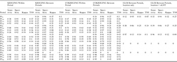
The variograms of each of the periods shown in Fig. 3 were used to predict both infections in the same period and infections in the next period (Table 1, first eight columns of numbers) by applying indicator kriging, assuming both spatial and temporal stationarity of the data within each time period and using a threshold value of 0·5.
Kriging and cokriging results of the analysis of the BTV-8 outbreak data. Periods (P1 to P5) refer to successive 20 day periods during the 2006 outbreak. Between 0% and 90% of the infected farm data were removed from the kriging calculations (e.g. P10 to P190) to examine how well these techniques are able to predict the missing data both in the same time period and in the next period (‘Within’ and ‘Between’ in the Table). The GLM results are shown for comparison with the kriging techniques. TSS = True Skill Statistic (see text)

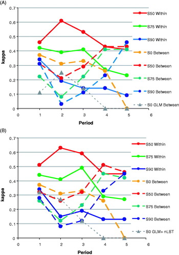
Predictions within each period were made based on kriging that used only 50%, 25% or 10% of the farms infected within that period to define the model variograms (in each case keeping to the observed values the proportions of infected to uninfected farms in the samples); predictions were then made for the 50%, 75% or 90% of omitted points within the same period. The aim here therefore was to see how well kriging ‘fills in’ the missing data. The results (first four columns of data in Table 1 and Fig. 4A) are expressed in terms of the model's sensitivity (proportion of correctly predicted positives), specificity (proportion of correctly predicted negative), True Skill Statistic, TSS (TSS = sensitivity + specificity – 1; (Allouche et al. Reference Allouche, Tsoar and Kadmon2006)) and kappa values. Kappa is an index of agreement that varies between −1 and +1, where 0 indicates a model fit no better than random and 1 indicates a perfect fit to the data (Congalton, Reference Congalton1991). Predictions for the following period used the same dataset from each period to predict the cases in the next period. To avoid the problem of exact prediction in kriging, the BT-negative data used to define the kriging weights were all those farms that were still negative at the end of the 20-day period being predicted. Again the model results are shown in terms of sensitivity, specificity, TSS and kappa values (data columns five to eight in Table 1). The kriging results in Table 1 are compared with the results from a commonly used aspatial modelling approach, Generalised Linear Models (GLM) (Table 1, columns 17 to 20). GLMs may also be spatial (Ben-Ahmed et al. Reference Ben-Ahmed, Bouratbine and El-Aroui2010), but are not commonly used as such.
Geo-statistical accuracy (kappa values) of predicting BTV-8 outbreak data within each 20-day period (Periods 1 to 5), or from one 20-day period to the next, when variable percentages (0%, 50%, 75% and 90%) of the BTV records are omitted from the calculations; A (upper) kriging and B (lower) cokriging using night-time Land Surface Temperature (nLST). For comparison both figures also show the results of applying a GLM to the infection data alone (A) or with nLST (B) to make predictions for the next 20-day period (data from Table 1).

Table 1 shows that between 26% (Period 2) and 99% (Period 5) of farms infected in the same period and between 12% (Period 2) and 98% (Period 5) of farms infected in the following interval were correctly predicted by the kriging. With the exception of Periods 4 and 5 ‘Between Periods’ results, model accuracies (kappa values) both within and between periods were greater the more data points were used to construct the model. TSS values tended to show the same trends. In contrast to the kriging approach, GLM methods performed poorly between periods, with kappa and TSS values below (Period 2) or well below (other periods) those produced by kriging (Table 1, data columns 17 to 20, and Fig. 4A).
Cokriging: the use and significance of co-varying environmental data
We might know from biological studies that a species or disease depends upon temperature in some way or other. It might therefore be argued that if we know the direct relationship between disease (y) and temperature (t) all we need is a high resolution map of temperature (such as those that may be derived from satellites) to predict the disease at any point (i) for which we have only temperature data, thus:
 $$y_i = f\,(t_i ) + \varepsilon _1 $$
where f(t) is some realistic function of temperature (derived directly from the sparse disease data) and ε 1 is a normally distributed error term. The ‘model’ in equation 7 is aspatial; we do not need to know conditions in any of the neighbouring pixels to make a prediction of y i. In describing this model we emphasised pre-existing biological knowledge, but equation 7 could also use predictor variables selected purely by data mining, which exploits statistical correlations between the species’ and environmental data. Even here, however, we hope that some of the variables selected by data mining may have biological significance of which we are currently unaware. Biologists analyzing pattern are always keen to identify underlying processes and the variables that drive them.
Spatial analysis using environmental covariates is relevant if the following equation gives us a better estimate of y i:
 $$y_i = \sum {w_d \cdot y_d + \sum {v_d \cdot t_d + \varepsilon _2}} $$
where w d and y d are the weights and the observations of the infection data as defined in equation 4 and v d and t d are respectively the weights and the observations of the same predictor environmental variable that was used in equation 7. Equation 8 defines one sort of cokriging (‘ordinary cokriging’) where knowledge of an intensively sampled variable (here the environmental variable, t) is used to predict the value of a less intensively sampled variable (here disease, y). The weights in equation 8 are derived by solving a system involving covariances (of y and t respectively) and the cross covariance (between y and t) (Goovaerts, Reference Goovaerts1997), with the conditions that the sum of w d =1 and the sum of v d = 0. The weights are found by expanding the kriging system of equation 5, which now includes both the variances C t,t and co-variances C y,t, and two Lagrange multipliers l y and l t :
 $$\scale99%\eqalign{& \left[ \matrix{C_{y,y} (y_1 - y_1 )\quad C_{y,y} (y_1 - y_2 )\quad C_{y,y} (y_1 - y_3 )\quad \quad C_{y,t} (y_1 - t_1 )\quad C_{y,t} (y_1 - t_2 )\quad C_{y,t} (y_1 - t_3 )\quad \quad \;1\quad 0 \cr C_{y,y} (y_2 - y_1 )\quad C_{y,y} (y_2 - y_2 )\quad C_{y,y} (y_2 - y_3 )\quad \quad C_{y,t} (y_2 - t_1 )\quad C_{y,t} (y_2 - t_2 )\quad C_{y,t} (y_2 - t_3 )\quad \quad 1\quad 0 \cr C_{y,y} (y_3 - y_1 )\quad C_{y,y} (y_3 - y_2 )\quad C_{y,y} (y_3 - y_3 )\quad \quad C_{y,t} (y_3 - t_1 )\quad C_{y,t} (y_3 - t_2 )\quad C_{y,t} (y_3 - t_3 )\quad \quad 1\quad 0 \cr \cr C_{y,t} (y_1 - t_1 )\quad C_{y,t} (y_1 - t_2 )\quad C_{y,t} (y_1 - t_3 )\quad \quad C_{t,t} (t_1 - t_1 )\quad C_{t,t} (t_1 - t_2 )\quad C_{t,t} (t_1 - t_3 )\quad \quad \quad \quad 0\quad 1 \cr C_{y,t} (y_2 - t_1 )\quad C_{y,t} (y_2 - t_2 )\quad C_{y,t} (y_2 - t_3 )\quad \quad C_{t,t} (t_2 - t_1 )\quad C_{t,t} (t_2 - t_2 )\quad C_{t,t} (t_2 - t_3 )\quad \quad \quad \;\;0\quad 1 \cr C_{y,t} (y_3 - t_1 )\quad C_{y,t} (y_3 - t_2 )\quad C_{y,t} (y_3 - t_3 )\quad \quad C_{t,t} (t_3 - t_1 )\quad C_{t,t} (t_3 - t_2 )\quad C_{t,t} (t_3 - t_3 )\quad \quad \quad \quad 0\quad 1 \cr \cr \quad \quad 1\quad \quad \quad \quad \quad \quad 1\quad \quad \quad \quad \quad \quad 1\quad \quad \quad \quad \quad \quad 0\quad \quad \quad \quad 0\quad \quad \quad \quad \quad \quad 0\quad {\kern 1pt} \quad {\kern 1pt} \quad {\kern 1pt} \quad {\kern 1pt} \quad {\kern 1pt} 0\quad {\kern 1pt} 0 \cr \quad \quad 0\quad \quad \quad \quad \quad \quad 0\quad \quad \quad \quad \quad \quad 0\quad \quad \quad \quad \quad \quad 1\quad \quad \quad \quad 1\quad \quad \quad \quad \quad \quad 1\quad {\kern 1pt} \quad {\kern 1pt} \quad {\kern 1pt} {\kern 1pt} \quad {\kern 1pt} \quad {\kern 1pt} 0\quad {\kern 1pt} 0} \right]\;\left[ \matrix{w_1 \hfill \cr w_2 \hfill \cr w_3 \hfill \cr \hfill \cr v_1 \hfill \cr v_2 \hfill \cr v_3 \hfill \cr \hfill \cr l_y \hfill \cr l_t \hfill} \right] \hskip-30pt\cr & = \;\left[ \matrix{C_{y,y} (y_i - y_1 ) \hfill \cr C_{y,y} (y_i - y_2 ) \hfill \cr C_{y,y} (y_i - y_3 ) \hfill \cr \hfill \cr C_{y,t} (y_i - t_1 ) \hfill \cr C_{y,t} (y_i - t_2 ) \hfill \cr C_{y,t} (y_i - t_3 ) \hfill \cr \hfill \cr 1 \hfill \cr 0 \hfill} \right]} $$
Had both variables in equation 8 been equally intensively sampled there would be no need for cokriging; kriging would give just as good a result. This is because the weights given to the secondary (predictor) variable tend to be small unless the primary variable is under-sampled in comparison with the secondary variable (Deutsch and Journel, Reference Deutsch and Journel1998).
Temperature appears in equation 8 not because it may be determining the species’ presence or absence but simply because it is sampled with a much higher intensity that is the species itself. The user may elect to use temperature because other studies suggest that temperature is important for the disease being modeled, but none of the various sorts of cokriging is able to distinguish potentially important from unimportant covariables, because they are not designed, and cannot be used, to do so (factorial cokriging identifies the spatial scale at which multivariate correlation is acting, and so may offer some guide to the biologically important variables; (Goovaerts, Reference Goovaerts1997)). Again the main reason here is because the covariances and cross covariances deal only with random errors (i.e. deviations from the respective means), not with the absolute values of either the disease or the environmental data. Cokriging exploits the correlation between the (random errors captured by the) model variograms (e.g. Fig. 2) and effectively uses the errors of the richly sampled data to predict the errors of the poorly sampled data in a purely statistical exercise.
If we ignore important spatial variation (e.g. by using equation 7 rather than equation 8) the variation in y that is captured by the covariates in equation 8 ends up in the error term, ε 1, of equation 7. A spatial plot of the residual errors from the fitting of equation 7 will reveal whether or not these residuals show any obvious spatial patterning. If they do, a spatial analysis is required.
Equations 7 and 8 can now be seen not as competing methods to describe the same phenomenon, but as complementary methods to describe spatial data. Equation 7 effectively describes a trend surface; variation of the mean of y i in response to the biologically important variable t. Equation 8 seeks to break down the error term of equation 7 into spatial and non-spatial components. The spatial component of error variance then joins the variance attributable to the linear relationship to give the total variance ‘explained’ by the model. Atkinson et al. (Reference Atkinson, Webster and Curran1994) point out that cokriging is profitable when there are similarities in the spatial patterns (cross-covariance) of the variable of interest and any environmental predictor variables, even when the direct correlation between the two is weak. Again this emphasises that kriging and cokriging are operations carried out on error terms that have a spatial component, and may have little or nothing to do with the functional dependence of one variable on another. Goovaerts and Kerry (Reference Goovaerts, Kerry and Oliver2010) compare cokriging with other multivariate geostatistical techniques.
Variation of environmental co-variables
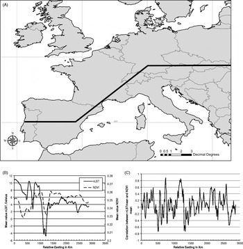
Environmental variables also vary through space. As an example, Fig. 5A shows a transect through Europe, and Fig. 5B shows the mean values of two environmental variables along this transect, the mean night-time Land Surface Temperature and the mean Normalised Difference Vegetation Index (NDVI) (both good statistical predictors of BTV-8 in aspatial models). Mean nLST decreases from West to East (with much variation associated with mountain ranges), whilst NDVI stays relatively constant. Fig. 5C shows the correlation between these two variables, which also varies spatially. Variation of this sort means that cokriging with environmental variables (equation 8) should be used with care; trending covariable data should be de-trended before they are used in any spatial analysis that assumes stationarity.
(A) Transect through Europe; (B) mean values of NDVI and night-time LST (nLST) in a 40 × 40 c.1 km pixel window moving along the transect, centred at the stated relative Eastings from the start of the transect on the coast of Portugal; (C) Correlation between nLST and NDVI along the transect. The trends and variability of the correlation between these variables requires pre-treatment of the data (i.e. detrending) followed by local cokriging.

The BTV-8 outbreak area covered the equivalent of only a small part of the transect shown in Fig. 5A. Fig. 2 also shows the variogram of nLST in the same region as the BTV-8 data. The nLST γ-variance rises rapidly with distance and the fitted variogram levels off at a range of about 250 km. The γ-variance of LST does not decrease beyond the range, as does the BTV-8 data, because LST is not spreading in the same way from a point or small-area source.
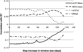
Can we exploit the correlation between the two sorts of variables in Fig. 2 to make better predictions of BTV-8, as suggested by equation 8? The answer to this question depends on how much the correlation between the environmental and disease data changes over time and space. For the BTV-8 outbreak data we have only one set of (temporal Fourier processed) satellite variables; hence any variability in the correlation between environmental and disease data comes from the variability of the disease data through time, not the satellite data. Fig. 6 shows the mean correlations of the BTV-8 outbreak data and four different environmental variables when the data were analysed by a window of progressively increasing size; size was increased by fixed amounts (called ‘steps’ in Fig. 6) and the correlations were calculated at each window size and then averaged for each of the incremental step lengths used. The environmental variables used were the biannual amplitude of the Middle Infra-Red (MIR), the annual amplitude of nLST, the mean nLST and the mean NDVI (again, these variables were chosen because statistical models of the BTV-8 data highlighted their potential importance). Thus, for example, a value of 2 on the x-axis of Fig. 6 means that the correlations were calculated of the BTV-8 and environmental data when the window included the disease data for days 0 to 2, 0 to 4, 0 to 6 and so on up to the end of the outbreak in December (in each case the BTV-8 negative data were farms infected after the windowed period). The correlations in this series were then averaged to give the value plotted in Fig. 6 at the incremental step of 2. All the other values plotted in Fig. 6 were produced in an analogous way, with different incremental steps. Clearly there were fewer values to average at the larger incremental values in Fig. 6. The figure shows considerable stability in the correlations of the BTV-8 data with each of the environmental variables (and regardless of the step increase) up to a step increase of about 40 days (beyond which the averages are based on very small sample sizes).
Correlation of environmental variables (mean night-time LST, mean NDVI, annual amplitude of night-time LST and bi-annual amplitude of Middle Infra Red (MIR)) with BTV-8 outbreak data within windows of increasing size during the 2006 outbreak. Windows were progressively increased by the amounts recorded on the x-axis (step increase). The y-axis records the average correlation for each series with each step increase.

Cokriging predictions of BTV-8 cases
Having established the statistical relationship between the disease and environmental data, how accurately can we predict disease in ‘unsampled’ places at the present time and into the future? We illustrate this topic again using the BTV-8 data by missing out 50, 75 and 90% of the BTV-8 records from the five different periods during the outbreak defined above. We seek to make predictions of infections within and between periods using only partial information (i.e. incomplete data) from the present period (Table 1, data columns 9 to 16 and Fig. 4B). We can therefore compare the results of cokriging with those of kriging (Figs. 4B and 4A respectively) to see the degree of improvement that cokriging offers.
Compared with the kriging results, cokriging produces an average percentage increase in kappa values of 9·7% (range −4·2% to +23·9%) within periods and 23·7% (range +2·4% to +80·2%) between periods across the different levels of data sub-sampling (Table 1 and Fig. 4B). The equivalent increases in TSS values are 14·5% (range −5·7% to +23·6%) and 12·1% (range −2·4% to +34·3%) respectively. Both sensitivity and specificity are improved by cokriging, the former more so (average percentage increases of 8·7% and 5·2% for within period predictions and 14·4 and −0·9% for between periods). Table 1 (data columns 21 to 24) and Fig. 4B also show the results of applying a GLM with both location and Land Surface Temperature as predictor variables (i.e. as in equation 7). The performance of the GLM with nLST is about the same as that of kriging in the early periods (1 and 2) but very much worse thereafter. It performs poorly because it is not incorporating any information about the spatial covariance of infections and nLST in its predictive process. The statistical advantages of kriging over GLM, and of cokriging over kriging, are therefore clear.
Overall the performance of kriging and co-kriging for the first three time periods was not very satisfactory. This was in part due to the use of data from periods when the disease outbreak had clearly not stabilised and in part due to the use of a series of spatial models instead of a full spatio-temporal model. Nevertheless we hope that several important principles were illustrated that will be of use to epidemiologists.
CONCLUSIONS
The key questions we need to ask when modelling species’ distributions are as follows: (1) What is of major interest, the pattern of a species’ distribution or the biological and other processes underlying (and eventually giving rise to) that pattern? (2) Which particular modelling approach is appropriate to reveal the subject of interest selected above? (3) Given that any model may eventually be used to make predictions of species or diseases in other times and/or places, which is the best road map through (1) and (2) to arrive at this destination?
We and others have previously called the pattern-matching modelling approach ‘statistical’ and the process-based modelling approach ‘biological’; whilst this polarization remains quite deep-seated in the modelling algorithms available to date this article tries to show how a combination of the two approaches potentially offers greater predictive skills through a statistically rigorous analysis of the data. Such an analysis considers the spatial context of the data, something which is missing from the majority of off-the-shelf algorithms available to date (Elith et al. Reference Elith, Graham, Anderson, Dudik, Ferrier, Guisan, Hijmans, Huettmann, Leathwick, Lehmann, Li, Lohmann, Loiselle, Manion, Moritz, Nakamura, Nakazawa, Overton, Townsend Peterson, Phillips, Richardson, Scachetti-Pereira, Schapire, Soberon, Williams, Wisz and Zimmermann2006).
Quite a few assumptions are involved in all kriging calculations and not all of them are always valid, especially for very variable biological data that usually have two quite different sources of variation, intrinsic and extrinsic. Intrinsic variation arises from some biological process such as birth and death, immigration and emigration or infection and recovery that commonly have spatial determinants. Birth rates vary locally and an area with a high population density is likely to send emigrants to nearby rather than remote areas; hence variation in population density is likely to be patchy at a scale much bigger than that of the individual sampling units. Extrinsic variation arises from the effect of the environment on a species’ or disease's occurrence. A variable such as temperature varies only slowly over space so that an area which is warm is more likely to be surrounded by warm rather than cold areas. Whilst this is likely to have effects on the biological processes determining species’ distributions it is of no consequence for kriging methods which deal only with the local values of disease and environmental data. A poor representation of the disease (due to inadequate sampling) may be enhanced through cokriging by a rich representation of co-varying environmental data to predict disease cases in unsampled places. If, however, there are equal numbers of disease and environmental data points in the local areas being kriged, the environmental data will have little influence on the cokriged predictions because they will have lower kriging weights than the disease data (for example, compare Table 1, data columns 7 and 15 for when no data are omitted, P10, P20, etc.; the kappa values are the same). Thus even though kriging methods potentially offer increased predictive accuracy (together with quantified errors) of species’ and diseases’ distribution patterns (key question 3 above), they cannot help us if we are really interested in understanding the biological processes underlying such spatial patterns (key questions 1 and 2 above).
Proper spatial analysis allows us to produce maps of species’ and disease risk with quantified errors and thus highlights areas of prediction uncertainty where new samples or studies are required. Kriging and cokriging methods should be applied to the production of risk maps more frequently than is the case at present so that users are presented with the best statistical description of the species’ or disease's current distribution. Biologists hoping for greater insight into processes will, however, be disappointed. The history of kriging, based as it is on mineral reserves, was never designed to answer the ‘Why?’, ‘When?’ and ‘How?’ questions that commonly confront biologists, only the ‘Where?’ questions important for mineral exploitation. Whilst the search for the Holy Grail of how to model species’ distributions continues, however, biologists can use geospatial techniques to refine their questions; that is, as a compass to take them in the right direction, but not as a map showing them their final destination.
ACKNOWLEDGEMENTS
The authors thank the Editors of Parasitology for their invitation to contribute to this Special Issue. We also thank the reviewers and, especially, Professor Emilio Porcu (Universidad de Valparaiso, Chile) for his comments and corrections of the early versions of this paper. This article is catalogued by the EDENext Steering Committee as EDENext042 (http://www.edenext.eu). The contents of this publication are the sole responsibility of the authors and do not necessarily reflect the views of the European Commission.
FINANCIAL SUPPORT
The authors are funded by a European Union grant FP7-261504, ‘EDENext’.