1 Introduction
Turbulent wind over water generates waves, which in turn alter the wind. The exchange of momentum, energy and mass occurring at air–water interfaces is to a large extent determined by this wind–wave interaction. Despite receiving constant attention from the research community in the form of field measurements (Hasselmann et al. Reference Hasselmann, Barnett, Bouws, Carlson, Cartwright, Enke, Ewing, Gienapp, Hasselmann and Kruseman1973; Hristov, Friehe & Miller Reference Hristov, Friehe and Miller1998; Edson et al. Reference Edson, Crawford, Crescenti, Farrar, Frew, Gerbi, Helmis, Hristov, Khelif and Jessup2007), laboratory experiments (Plant Reference Plant1982; Mastenbroek et al. Reference Mastenbroek, Makin, Garat and Giovanangeli1996; Grare et al. Reference Grare, Peirson, Branger, Walker, Giovanangeli and Makin2013; Buckley & Veron Reference Buckley and Veron2016), theoretical studies (Miles Reference Miles1957; Phillips Reference Phillips1957; Janssen Reference Janssen1991; Belcher & Hunt Reference Belcher and Hunt1993) and numerical simulations (Gent & Taylor Reference Gent and Taylor1976; Van Duin & Janssen Reference Van Duin and Janssen1992; Li, Xu & Taylor Reference Li, Xu and Taylor2000; Meirink & Makin Reference Meirink and Makin2000; Sullivan, McWilliams & Moeng Reference Sullivan, McWilliams and Moeng2000; Sullivan et al. Reference Sullivan, Edson, Hristov and McWilliams2008; Yang, Meneveau & Shen Reference Yang, Meneveau and Shen2013), there are still some very simple questions that remain only partly answered. One of these questions is how the form drag, exerted by the waves on the air, depends on the properties of the air flow and the waves.
Naturally, early attempts at numerical modelling of this flow were devoted to the use of Reynolds averaged Navier–Stokes (RANS) models for monochromatic waves (Gent & Taylor Reference Gent and Taylor1976; Van Duin & Janssen Reference Van Duin and Janssen1992). The results turned out to be sensitive to the choice of turbulence closure scheme (Van Duin & Janssen Reference Van Duin and Janssen1992), and suitable closures were adopted (Mastenbroek et al. Reference Mastenbroek, Makin, Garat and Giovanangeli1996; Li et al. Reference Li, Xu and Taylor2000; Meirink & Makin Reference Meirink and Makin2000). Increased computing capabilities led to the advent of direct numerical simulation (DNS) studies (Sullivan et al. Reference Sullivan, McWilliams and Moeng2000; Kihara, Mizuya & Ueda Reference Kihara, Mizuya and Ueda2007; Yang & Shen Reference Yang and Shen2009, Reference Yang and Shen2010). DNS studies have provided valuable insight into the shape of the wave-correlated motion (Sullivan et al. Reference Sullivan, McWilliams and Moeng2000) and the structure of the turbulence (Yang & Shen Reference Yang and Shen2009, Reference Yang and Shen2010). Due to the strict resolution requirements inherent to DNS, only low Reynolds numbers have been considered so far. Meirink & Makin (Reference Meirink and Makin2000) used RANS models suitable for low Reynolds number flows to discuss the Reynolds number effects on the drag. They found reasonable agreement with Sullivan et al. (Reference Sullivan, McWilliams and Moeng2000) at low Reynolds number, but further showed that there are considerable differences between the form drag obtained at low and intermediate Reynolds numbers. Large eddy simulation (LES) studies have primarily been aimed at closing the gap to operational models, with special attention given to subgrid near-surface modelling and the inclusion of a realistic wave spectrum (Sullivan et al. Reference Sullivan, Edson, Hristov and McWilliams2008; Yang et al. Reference Yang, Meneveau and Shen2013; Hara & Sullivan Reference Hara and Sullivan2015). However, Yang et al. (Reference Yang, Meneveau and Shen2013) used wall resolved LES at an intermediate to high Reynolds number as a baseline for their discussions on subgrid modelling.
Waves that are slower than the bulk wind extract momentum from the wind through the action of the wave-correlated pressure against the slope of the surface. These waves are responsible for most of the momentum transfer from the atmosphere to the sea. In this part of the spectrum, breaking is frequent, which increases both drag and aerosol transport (Donelan Reference Donelan and Imberger1998). Operational wave forecasting relies on the celebrated critical layer mechanism of Miles (Reference Miles1957, Reference Miles1959), where the discontinuity in wave-correlated Reynolds stresses at the critical layer is responsible for resonance. The existence of the critical layer, and the corresponding jump in wave-correlated Reynolds stresses, has been demonstrated both numerically (Sullivan et al. Reference Sullivan, McWilliams and Moeng2000) and in field observations (Hristov, Miller & Friehe Reference Hristov, Miller and Friehe2003). However, Belcher & Hunt (Reference Belcher and Hunt1993, Reference Belcher and Hunt1998) argued on the basis of a rapid distortion framework, that the Miles mechanism could only be active for relatively fast waves and reintroduced a non-separated version of the Jeffreys (Reference Jeffreys1925) sheltering mechanism for slow waves.
Waves that propagate faster than the bulk wind typically emerge as the result of nonlinear interaction of slower waves, or as the result of distantly storm-generated waves that enter domains of lighter winds. The momentum flux between the air and the sea is dramatically altered in the presence of fast moving waves (Sullivan et al. Reference Sullivan, Edson, Hristov and McWilliams2008; Kahma et al. Reference Kahma, Donelan, Drennan and Terray2016). In severe situations, fast waves even have the ability to generate wind (see for instance Semedo et al. Reference Semedo, Saetra, Rutgersson, Kahma and Pettersson2009). Examples of simplified models for the air-side response in this regime include Cohen & Belcher (Reference Cohen and Belcher1999), Kudryavtsev & Makin (Reference Kudryavtsev and Makin2004) and Semedo et al. (Reference Semedo, Saetra, Rutgersson, Kahma and Pettersson2009).
In the present work, we perform wall resolved LES over monochromatic waves for different wave ages and Reynolds numbers. With wall resolved LES the requirements for resolving the turbulence in an adequate manner are less severe than in DNS, and as such, it may be a valuable tool for studying the flow dynamics in the intermediate Reynolds number range. The layout of this paper is as follows: § 2 contains the problem formulation and a description of the mathematical tools used. In § 3 we analyse the LES results in terms of Reynolds number and wave age dependence. Both the mean and the fundamental mode momentum balances are investigated to quantify the relevance of the different stresses involved. The LES results point towards the existence of a quasi-laminar regime at intermediate to high wave ages, characterised by a balance between viscous and wave-induced stresses. Therefore, in § 4, we tentatively perform a splitting of the flow field into a laminar wave-generated response (Lamb Reference Lamb1932), and a turbulent shear flow. The former is driven by the non-homogeneous boundary conditions, whereas the latter is driven by a constant volume force, turbulent stresses and the laminar solution. We approach the problem in the opposite direction compared to, for instance, Miles (Reference Miles1957), where the wave-correlated motion is found by linearisation about an estimated mean flow. The aim of the present formulation is to emphasise the role of the simple wave-induced motion for intermediate to high wave ages and explore the possibility of linear solutions in the resulting wave-correlated flow fields. With linear solutions, we mean linear in the sense of a flat boundary layer; while turbulent fluctuations are active at all scales, we investigate whether or not the wave-correlated mean flow associated with the turbulent shear flow interacts with itself.
2 Problem formulation
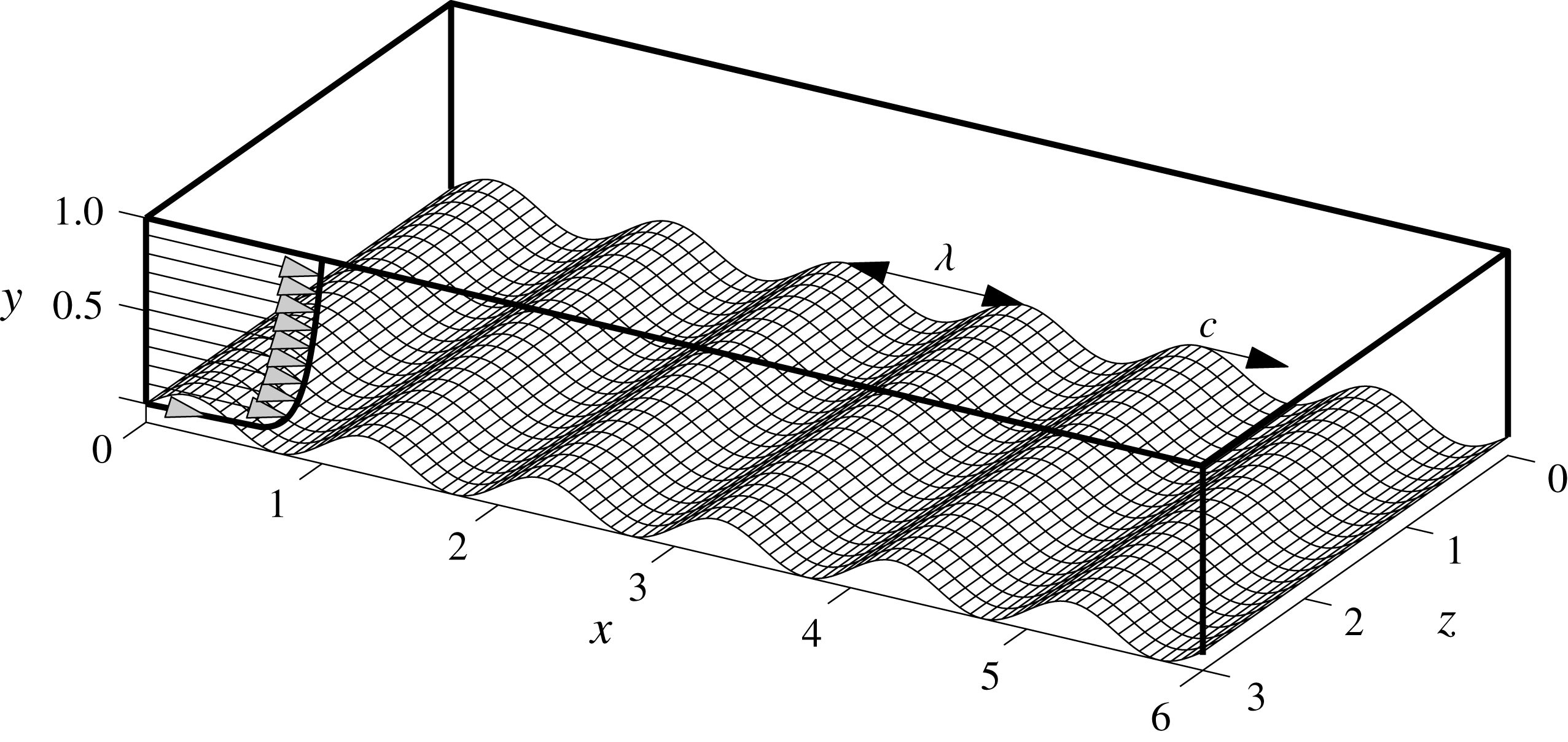
Illustration of computational domain.

A fully developed pressure-driven open channel flow with a moving lower wavy surface is considered. Figure 1 gives an illustration of the set-up. The domain size is
 $(L_{x},L_{y},L_{z})=(6,1,3)$
wavelengths in the streamwise, vertical and cross-stream directions, respectively. The lower surface is described by a propagating wave
 $y=\unicode[STIX]{x1D702}(x,t)=a\sin (k(x-ct))$
with amplitude
 $a$
, wavenumber
 $k=2\unicode[STIX]{x03C0}/\unicode[STIX]{x1D706}$
and phase velocity
 $c$
. At this boundary, the flow is subject to kinematic boundary conditions from the wave orbital movement imposed by the propagating wave. In the frame of reference that moves with the propagating wave, the wave shape and the wave orbital velocities are stationary, i.e.
 $$\begin{eqnarray}\displaystyle (u,v,w)_{y=\unicode[STIX]{x1D702}(x)}=(akc\sin (kx)-c,-akc\cos (kx),0). & & \displaystyle\end{eqnarray}$$
At the top boundary, slip conditions are prescribed, whereas in the streamwise and cross-stream directions periodicity is imposed. The fluid motion is described by the incompressible Navier–Stokes equations
 $$\begin{eqnarray}\displaystyle & \displaystyle \unicode[STIX]{x2202}_{t}u_{i}+u_{j}\unicode[STIX]{x2202}_{j}u_{i}=-\unicode[STIX]{x2202}_{i}p+\unicode[STIX]{x2202}_{j}2\unicode[STIX]{x1D708}_{t}\unicode[STIX]{x1D634}_{ij}+\frac{{\hat{u} _{\unicode[STIX]{x1D70F}}}^{2}}{h}\unicode[STIX]{x1D6FF}_{1i}, & \displaystyle\end{eqnarray}$$
 $$\begin{eqnarray}\displaystyle & \displaystyle \unicode[STIX]{x2202}_{i}u_{i}=0, & \displaystyle\end{eqnarray}$$
 $x_{i}=(x_{1},x_{2},x_{3})=(x,y,z)$
denotes the streamwise, vertical and cross-stream coordinates, respectively. The velocities in the corresponding directions are
 $u_{i}=(u_{1},u_{2},u_{3})=(u,v,w)$
. In the above equations, the summation convention applies to repeated indices, and
 $\unicode[STIX]{x1D6FF}_{1i}$
is the Kronecker delta function. The constant density is absorbed into the pressure,
 $p$
, and the volume force,
 ${\hat{u} _{\unicode[STIX]{x1D70F}}}^{2}/h$
. This volume force is defined as in Kihara et al. (Reference Kihara, Mizuya and Ueda2007), using a virtual friction velocity
 $\hat{u} _{\unicode[STIX]{x1D70F}}$
at the surface and the channel half height
 $h$
. As in that work, we keep
 $\hat{u} _{\unicode[STIX]{x1D70F}}=1$
for all Reynolds numbers and wave ages, and the actual computed friction velocity,
 $u_{\unicode[STIX]{x1D70F}}$
, as given later in equation (3.3), is almost identical to this virtually defined friction velocity for all cases considered. Furthermore, the traceless strain-rate tensor is
 $\unicode[STIX]{x1D634}_{ij}=1/2(\unicode[STIX]{x2202}_{j}u_{i}+\unicode[STIX]{x2202}_{i}u_{j})$
and we have allowed for a varying kinematic viscosity,
 $\unicode[STIX]{x1D708}_{t}(x_{i},t)=\unicode[STIX]{x1D708}+\unicode[STIX]{x1D708}_{sgs}(x_{i},t)$
, where
 $\unicode[STIX]{x1D708}$
is the kinematic viscosity of the fluid and
 $\unicode[STIX]{x1D708}_{sgs}(x_{i},t)$
is the subgrid viscosity from the LES closure model.
2.1 Averaging, RANS and Fourier transform
For analysis, the simulation results are averaged in the cross-stream direction and time, thus enabling the Reynolds decomposition
 $$\begin{eqnarray}\displaystyle u_{i}(x_{j},t)=\langle u_{i}(x_{j},t)\rangle +u_{i}^{\prime }(x_{j},t)=U_{i}(x,y)+u_{i}^{\prime }(x_{j},t),\quad p(x_{j},t)=P(x,y)+p^{\prime }(x_{j},t). & & \displaystyle \nonumber\\ \displaystyle & & \displaystyle\end{eqnarray}$$
For simplicity, throughout the rest of the paper we will let
 $(u,v,p)$
refer to the mean velocity field
 $(U(x,y)+c,V(x,y),P(x,y))$
and
 $(u_{i}^{\prime },p^{\prime })$
refer to the turbulent fluctuations. In the frame of reference moving with the wave, the Reynolds averaged Navier–Stokes formulation of (2.2) is
 $$\begin{eqnarray}\displaystyle & \displaystyle (u-c)\unicode[STIX]{x2202}_{x}u+v\unicode[STIX]{x2202}_{y}u=-\unicode[STIX]{x2202}_{x}p+\unicode[STIX]{x1D708}\unicode[STIX]{x1D6FB}^{2}u-\unicode[STIX]{x2202}_{x}\langle u^{\prime }u^{\prime }\rangle -\unicode[STIX]{x2202}_{y}\langle u^{\prime }v^{\prime }\rangle +{\hat{u} _{\unicode[STIX]{x1D70F}}}^{2}/h, & \displaystyle\end{eqnarray}$$
 $$\begin{eqnarray}\displaystyle & \displaystyle (u-c)\unicode[STIX]{x2202}_{x}v+v\unicode[STIX]{x2202}_{y}v=-\unicode[STIX]{x2202}_{y}p+\unicode[STIX]{x1D708}\unicode[STIX]{x1D6FB}^{2}v-\unicode[STIX]{x2202}_{x}\langle u^{\prime }v^{\prime }\rangle -\unicode[STIX]{x2202}_{y}\langle v^{\prime }v^{\prime }\rangle , & \displaystyle\end{eqnarray}$$
 $$\begin{eqnarray}\displaystyle & \displaystyle \unicode[STIX]{x2202}_{x}u+\unicode[STIX]{x2202}_{y}v=0, & \displaystyle\end{eqnarray}$$
 $\langle u_{i}^{\prime }u_{j}^{\prime }\rangle$
are the Reynolds stresses. In the above equations, the subgrid eddy viscosity terms have not been included, because their contribution to the momentum balances considered in the rest of the paper is small.
To aid the analysis, the RANS equations are Fourier transformed in the streamwise direction. This may be achieved by first mapping the physical curved domain into a rectangular domain by the transformation
 $$\begin{eqnarray}\displaystyle \unicode[STIX]{x1D712}=x,\quad \unicode[STIX]{x1D709}=y-g(\unicode[STIX]{x1D712},\unicode[STIX]{x1D709})=y-\frac{ai}{2}(\exp (-\text{i}k\unicode[STIX]{x1D712})-\exp (\text{i}k\unicode[STIX]{x1D712}))\exp (-k\unicode[STIX]{x1D709}). & & \displaystyle\end{eqnarray}$$
In this coordinate system the RANS equations (2.4) can be approximated by
 $$\begin{eqnarray}\displaystyle & \displaystyle (u-c)\unicode[STIX]{x2202}_{\unicode[STIX]{x1D712}}u+v\unicode[STIX]{x2202}_{\unicode[STIX]{x1D709}}u=-\unicode[STIX]{x2202}_{\unicode[STIX]{x1D712}}p+\unicode[STIX]{x1D708}\unicode[STIX]{x1D6FB}_{\unicode[STIX]{x1D712}}^{2}u-\unicode[STIX]{x2202}_{\unicode[STIX]{x1D712}}\langle u^{\prime }u^{\prime }\rangle -\unicode[STIX]{x2202}_{\unicode[STIX]{x1D709}}\langle u^{\prime }v^{\prime }\rangle +{\hat{u} _{\unicode[STIX]{x1D70F}}}^{2}/h+{\mathcal{L}}_{u}+\unicode[STIX]{x1D708}{\mathcal{L}}_{N}u,\qquad & \displaystyle\end{eqnarray}$$
 $$\begin{eqnarray}\displaystyle & \displaystyle (u-c)\unicode[STIX]{x2202}_{\unicode[STIX]{x1D712}}v+v\unicode[STIX]{x2202}_{\unicode[STIX]{x1D709}}v=-\unicode[STIX]{x2202}_{\unicode[STIX]{x1D709}}p+\unicode[STIX]{x1D708}\unicode[STIX]{x1D6FB}_{\unicode[STIX]{x1D712}}^{2}v-\unicode[STIX]{x2202}_{\unicode[STIX]{x1D712}}\langle u^{\prime }v^{\prime }\rangle -\unicode[STIX]{x2202}_{\unicode[STIX]{x1D709}}\langle v^{\prime }v^{\prime }\rangle +{\mathcal{L}}_{v}+\unicode[STIX]{x1D708}{\mathcal{L}}_{N}v, & \displaystyle\end{eqnarray}$$
 $$\begin{eqnarray}\displaystyle & \displaystyle \unicode[STIX]{x2202}_{\unicode[STIX]{x1D712}}u+\unicode[STIX]{x2202}_{\unicode[STIX]{x1D709}}v=g_{\unicode[STIX]{x1D712}}\unicode[STIX]{x2202}_{\unicode[STIX]{x1D709}}u, & \displaystyle\end{eqnarray}$$
 $$\begin{eqnarray}\displaystyle \unicode[STIX]{x1D6FB}_{\unicode[STIX]{x1D712}}^{2}=\frac{\unicode[STIX]{x2202}^{2}}{\unicode[STIX]{x2202}\unicode[STIX]{x1D712}^{2}}+\frac{\unicode[STIX]{x2202}^{2}}{\unicode[STIX]{x2202}\unicode[STIX]{x1D709}^{2}},\quad {\mathcal{L}}_{N}=g_{\unicode[STIX]{x1D712}}^{2}\frac{\unicode[STIX]{x2202}^{2}}{\unicode[STIX]{x2202}\unicode[STIX]{x1D709}^{2}}-2g_{\unicode[STIX]{x1D712}}\frac{\unicode[STIX]{x2202}^{2}}{\unicode[STIX]{x2202}\unicode[STIX]{x1D712}\unicode[STIX]{x2202}\unicode[STIX]{x1D709}}+(g_{\unicode[STIX]{x1D712}}g_{\unicode[STIX]{x1D712}\unicode[STIX]{x1D709}}-g_{\unicode[STIX]{x1D712}\unicode[STIX]{x1D712}})\frac{\unicode[STIX]{x2202}}{\unicode[STIX]{x2202}\unicode[STIX]{x1D709}}, & & \displaystyle\end{eqnarray}$$
and
 $$\begin{eqnarray}\displaystyle {\mathcal{L}}_{u}=(u-c)g_{\unicode[STIX]{x1D712}}\unicode[STIX]{x2202}_{\unicode[STIX]{x1D709}}u+g_{\unicode[STIX]{x1D712}}\unicode[STIX]{x2202}_{\unicode[STIX]{x1D709}}p+g_{\unicode[STIX]{x1D712}}\unicode[STIX]{x2202}_{\unicode[STIX]{x1D709}}\langle u^{\prime }u^{\prime }\rangle ,\quad {\mathcal{L}}_{v}=(u-c)g_{\unicode[STIX]{x1D712}}\unicode[STIX]{x2202}_{\unicode[STIX]{x1D709}}v+g_{\unicode[STIX]{x1D712}}\unicode[STIX]{x2202}_{\unicode[STIX]{x1D709}}\langle u^{\prime }v^{\prime }\rangle .\qquad & & \displaystyle\end{eqnarray}$$
Here, we have used the approximation
 $\unicode[STIX]{x2202}_{y}=(1-g_{\unicode[STIX]{x1D709}})^{-1}\unicode[STIX]{x2202}_{\unicode[STIX]{x1D709}}\approx \unicode[STIX]{x2202}_{\unicode[STIX]{x1D709}}$
. Strictly, this requires a lower wave steepness than what is considered here, but for analysis purposes it is more convenient to use the simplified expression. In § 4.3, where a numerical solution to the system is sought, the full expression is used.
The variables are expanded in multiples of the fundamental mode,
 $$\begin{eqnarray}\displaystyle f(\unicode[STIX]{x1D712},\unicode[STIX]{x1D709})=\mathop{\sum }_{m=-M}^{M}\hat{f}_{m}(\unicode[STIX]{x1D709})\exp (\text{i}km\unicode[STIX]{x1D712}),\quad \hat{f}_{-m}=\hat{f}_{m}^{\ast }, & & \displaystyle\end{eqnarray}$$
where
 $\hat{f}$
denotes the complex Fourier amplitude function and
 $M$
is the number of modes. The fundamental mode is
 $m=\pm 1$
, the purely real zero component, or mean, is
 $m=0$
and higher harmonics are
 $m=\pm 2,\pm 3,\ldots .$
Nonlinear advection terms and terms involving
 $g_{\unicode[STIX]{x1D712}}$
, henceforth referred to as geometric terms due to their link to the surface shape, both give rise to convolution terms. Note specifically that advection terms involving
 $\unicode[STIX]{x2202}_{x}$
transform to
 $$\begin{eqnarray}\displaystyle {\mathcal{F}}(f\unicode[STIX]{x2202}_{x}h)\simeq {\mathcal{F}}(f\unicode[STIX]{x2202}_{\unicode[STIX]{x1D712}}h-fg_{\unicode[STIX]{x1D712}}\unicode[STIX]{x2202}_{\unicode[STIX]{x1D709}}h)={\mathcal{F}}(f)\ast ({\mathcal{F}}(\unicode[STIX]{x2202}_{\unicode[STIX]{x1D712}}h)-{\mathcal{F}}(g_{\unicode[STIX]{x1D712}}\unicode[STIX]{x2202}_{\unicode[STIX]{x1D709}}h)). & & \displaystyle\end{eqnarray}$$
Since the function
 $g(\unicode[STIX]{x1D712},\unicode[STIX]{x1D709})$
is periodic with wavenumber
 $k$
, the Fourier transform of the last term leads to a coupling with higher and lower harmonics,
 $$\begin{eqnarray}\displaystyle {\mathcal{F}}(g_{\unicode[STIX]{x1D712}}\unicode[STIX]{x2202}_{\unicode[STIX]{x1D709}}h)_{m}=\frac{ak}{2}\exp (-k\unicode[STIX]{x1D709}){\mathcal{D}}({\hat{h}}_{m-1}+{\hat{h}}_{m+1})={\mathcal{D}}_{g}({\hat{h}}_{m-1}+{\hat{h}}_{m+1})={\mathcal{D}}_{g}[{\hat{h}}_{m}]. & & \displaystyle\end{eqnarray}$$
Throughout the rest of the paper the
 $\unicode[STIX]{x1D709}-$
derivative will be denoted
 $\unicode[STIX]{x2202}_{\unicode[STIX]{x1D709}}={\mathcal{D}}$
and the shorthand notation for the geometric coupling contribution
 ${\mathcal{D}}_{g}[{\hat{h}}_{m}]$
will be used. The continuity equation (2.4c
) for mode
 $m$
is then simply
 $$\begin{eqnarray}\displaystyle \text{i}km\hat{u} _{m}-{\mathcal{D}}_{g}[\hat{u} _{m}]+{\mathcal{D}}\hat{v}_{m}=0, & & \displaystyle\end{eqnarray}$$
and the
 $m$
th mode of an advection term can be expressed as
 $$\begin{eqnarray}\displaystyle & & \displaystyle {\mathcal{F}}(f\unicode[STIX]{x2202}_{\unicode[STIX]{x1D712}}h-fg_{\unicode[STIX]{x1D712}}\unicode[STIX]{x2202}_{\unicode[STIX]{x1D709}}h)_{m}=\hat{f}_{0}(\text{i}mk{\hat{h}}_{m}-{\mathcal{D}}_{g}[{\hat{h}}_{m}])\nonumber\\ \displaystyle & & \displaystyle \quad +\,\hat{f}_{-1}(\text{i}(m+1)k{\hat{h}}_{m+1}-{\mathcal{D}}_{g}[{\hat{h}}_{m+1}])+\hat{f}_{1}(\text{i}(m-1)k{\hat{h}}_{m-1}-{\mathcal{D}}_{g}[{\hat{h}}_{m-1}])+\cdots \qquad\end{eqnarray}$$
By application of the above two relations, the momentum equations (2.4a ) and (2.4b ) can be transformed to
 $$\begin{eqnarray}\displaystyle \text{i}km(\widehat{uu}_{m}-c\hat{u} _{m})+{\mathcal{D}}\widehat{uv}_{m} & = & \displaystyle \text{i}km(\text{i}km\unicode[STIX]{x1D708}\hat{u} _{m}-\hat{p}_{m}-\widehat{\langle u^{\prime }u^{\prime }\rangle }_{m})+{\mathcal{D}}(\unicode[STIX]{x1D708}{\mathcal{D}}\hat{u} _{m}-\widehat{\langle u^{\prime }v^{\prime }\rangle }_{m})\nonumber\\ \displaystyle & & \displaystyle +\,{\hat{u} _{\unicode[STIX]{x1D70F}}}^{2}/h\unicode[STIX]{x1D6FF}_{0m}+{\mathcal{D}}_{g}[\widehat{\langle u^{\prime }u^{\prime }\rangle }_{m}+\hat{p}_{m}+\widehat{uu}_{m}-c\hat{u} _{m}],\end{eqnarray}$$
 $$\begin{eqnarray}\displaystyle \text{i}km(\widehat{uv}_{m}-c\hat{v}_{m})+{\mathcal{D}}\widehat{vv}_{m} & = & \displaystyle \text{i}km(\unicode[STIX]{x1D708}\text{i}km\hat{v}_{m}-\widehat{\langle u^{\prime }v^{\prime }\rangle }_{m})+{\mathcal{D}}(\unicode[STIX]{x1D708}{\mathcal{D}}\hat{v}_{m}-\hat{p}_{m}-\widehat{\langle v^{\prime }v^{\prime }\rangle }_{m})\nonumber\\ \displaystyle & & \displaystyle +\,{\mathcal{D}}_{g}[\widehat{\langle u^{\prime }v^{\prime }\rangle }_{m}+\widehat{uv}_{m}-c\hat{v}_{m}].\end{eqnarray}$$
These equations have been cast in conservative form in order to simplify the identification of the various stresses in the flow. Since the wave-correlated stresses are nonlinear terms, they couple higher and lower harmonics. This can be seen from the expansion of the wave-correlated shear stress
 $$\begin{eqnarray}\displaystyle \widehat{uv}_{m}=\hat{u} _{0}\hat{v}_{m}+\hat{u} _{-1}\hat{v}_{m+1}+\hat{u} _{1}\hat{v}_{m-1}+\hat{u} _{-2}\hat{v}_{m+2}+\hat{u} _{2}\hat{v}_{m-2}+\cdots & & \displaystyle\end{eqnarray}$$
The geometrical correction,
 ${\mathcal{D}}_{g}$
, to the streamwise derivative also introduces a coupling between higher and lower harmonics, even for linear terms such as pressure, as seen from equation (2.11). In equations (2.14) and (2.15), the geometry corrections to the Laplacian have been omitted. We have verified numerically that their contributions to the analysis performed in subsequent sections are negligible.
There is a difference in the way the wave-correlated stresses and the Reynolds stresses are treated. The wave-correlated stresses are inherently mean flow quantities. Therefore, these stresses are obtained as products of the individual Fourier components of the mean flow. On the other hand, the Reynolds stresses are turbulent quantities and their individual modes,
 $\widehat{\langle u_{i}^{\prime }u_{j}^{\prime }\rangle }_{m}$
, can only be accessed from a Fourier transform of
 $\langle u_{i}^{\prime }u_{j}^{\prime }\rangle$
.
3 Large eddy simulation
3.1 Numerical method
The Navier–Stokes equations (2.2) are solved by means of LES, using the unstructured finite-volume node-based solver VIDA from Cascade Technologies (see for instance Ham, Mattsson & Iaccarino Reference Ham, Mattsson and Iaccarino2006; Ham et al.
Reference Ham, Mattsson, Iaccarino, Moin, Kassinos, Langer, Iaccarino and Moin2007). LES subgrid terms are modelled by means of a dynamic Smagorinsky procedure suitable for unstructured grids, as described in Mahesh, Constantinescu & Moin (Reference Mahesh, Constantinescu and Moin2004). The equations are advanced in time using the second-order BDF-2 scheme, and a fractional step predictor–corrector procedure is employed to ensure conservation of mass. The computational grid is generated by first considering a rectangular domain with coordinates
 $(\unicode[STIX]{x1D712},\unicode[STIX]{x1D709},\unicode[STIX]{x1D701})$
. Uniform spacing is imposed in the two horizontal directions (
 $\unicode[STIX]{x1D712}$
and
 $\unicode[STIX]{x1D701}$
) and a grid stretching is applied in the vertical direction (
 $\unicode[STIX]{x1D709}$
). For all cases, the average grid spacing in viscous units along the surface is
 $\unicode[STIX]{x0394}\unicode[STIX]{x1D709}^{+}=\unicode[STIX]{x0394}\unicode[STIX]{x1D709}_{min}u_{\unicode[STIX]{x1D70F}}/\unicode[STIX]{x1D708}=0.7\unicode[STIX]{x1D708}/u_{\unicode[STIX]{x1D70F}}$
. A transformation to physical space is obtained by means of
 $$\begin{eqnarray}\displaystyle x=\unicode[STIX]{x1D712},\quad y=\unicode[STIX]{x1D702}(\unicode[STIX]{x1D712})+\unicode[STIX]{x1D709}(1-\unicode[STIX]{x1D702}(\unicode[STIX]{x1D712})/h),\quad z=\unicode[STIX]{x1D701}, & & \displaystyle\end{eqnarray}$$
where
 $\unicode[STIX]{x1D709}\in [0,h]$
, and
 $\unicode[STIX]{x1D702}(\unicode[STIX]{x1D712})$
is the surface deformation. This results in an
 $O(a/h)$
variation of the grid spacing over a wavelength close to the surface. Furthermore, since there is surface stress variation over a wavelength, the effective viscous grid spacing close to the surface varies from
 $\unicode[STIX]{x0394}y^{+}\approx 0.2$
to
 $\unicode[STIX]{x0394}y^{+}\approx 1.5$
. Note that this transformation is different from the one used in to transform the equations for analysis. The grid spacing is comparable to previous DNS studies (Sullivan et al.
Reference Sullivan, McWilliams and Moeng2000; Kihara et al.
Reference Kihara, Mizuya and Ueda2007; Yang & Shen Reference Yang and Shen2010). However, we use a second-order finite-volume framework, which for the same grid spacing is not expected to resolve the physics as accurately as the pseudo-spectral methods used in previous DNS studies (see for instance Boyd (Reference Boyd2001) for differences in global versus local approximation methods). Therefore, we have used LES to account for unresolved turbulent fluctuations.
The flow over the waves depends on both the wave friction Reynolds number,
 $Re_{\unicode[STIX]{x1D70F}}=u_{\unicode[STIX]{x1D70F}}\unicode[STIX]{x1D706}/\unicode[STIX]{x1D708}$
, henceforth referred to as the Reynolds number, and the wave age,
 $c/u_{\unicode[STIX]{x1D70F}}$
. The simulations cover a range of wave ages for the three Reynolds numbers
 $Re_{\unicode[STIX]{x1D70F}}=\{200,395,950\}$
. In addition, a simulation at
 $c/u_{\unicode[STIX]{x1D70F}}=4$
with
 $Re_{\unicode[STIX]{x1D70F}}=260$
was performed in order to compare with the shear-driven flow of Sullivan et al. (Reference Sullivan, McWilliams and Moeng2000). Table 1 shows the details of the different simulations.
3.2 Mean flow description
Colour contours of pressure
 $akp/{u_{\unicode[STIX]{x1D70F}}}^{2}$
and streamlines of the mean flow (——) for (a)
 $Re_{\unicode[STIX]{x1D70F}}=200$
at
 $c/u_{\unicode[STIX]{x1D70F}}=4$
, (b)
 $Re_{\unicode[STIX]{x1D70F}}=950$
at
 $c/u_{\unicode[STIX]{x1D70F}}=4$
, (c)
 $Re_{\unicode[STIX]{x1D70F}}=200$
at
 $c/u_{\unicode[STIX]{x1D70F}}=16$
and (d)
 $Re_{\unicode[STIX]{x1D70F}}=950$
at
 $c/u_{\unicode[STIX]{x1D70F}}=16$
. The critical layer, i.e. where
 $u=c$
, is shown as (

 $akp/{u_{\unicode[STIX]{x1D70F}}}^{2}=-0.6$
(dark blue) to
 $akp/{u_{\unicode[STIX]{x1D70F}}}^{2}=0.6$
(bright red) with an increment of
 $0.2$
. The zero contour is located between white and blue.

Computation cases. All cases use a geometric stretching in the vertical direction of
 $r=1.03$
and the spacing from the surface to the first point in the domain is
 $\unicode[STIX]{x0394}\unicode[STIX]{x1D709}_{min}u_{\unicode[STIX]{x1D70F}}/\unicode[STIX]{x1D708}=0.7$
.

An illustration of how the flow field varies with Reynolds number and wave age is found in figure 2. It contains pressure contours and mean flow streamlines for combinations of two wave ages (
 $c/u_{\unicode[STIX]{x1D70F}}=4$
and
 $16$
) and two Reynolds numbers (
 $Re_{\unicode[STIX]{x1D70F}}=200$
and
 $950$
). The critical layer, i.e. where the streamwise velocity
 $u$
matches the wave speed
 $c$
, is shown as (

An increase in wave age shifts the location of the cat’s-eye outwards. On the other hand, an increase in Reynolds number compresses the mean flow profile towards the surface as the boundary layer becomes steeper. In viscous units, however, the critical layer position is almost constant for low wave ages. Specifically, for the wave age
 $c/u_{\unicode[STIX]{x1D70F}}=4$
, the critical layer location is
 $\unicode[STIX]{x1D709}u_{\unicode[STIX]{x1D70F}}/\unicode[STIX]{x1D708}\approx 5$
for all Reynolds numbers considered. For higher wave ages, the critical layer location increases with Reynolds number, and for
 $c/u_{\unicode[STIX]{x1D70F}}=16$
its location ranges from
 $\unicode[STIX]{x1D709}u_{\unicode[STIX]{x1D70F}}/\unicode[STIX]{x1D708}\approx 40$
for
 $Re_{\unicode[STIX]{x1D70F}}=200$
to
 $\unicode[STIX]{x1D709}u_{\unicode[STIX]{x1D70F}}/\unicode[STIX]{x1D708}\approx 60$
for
 $Re_{\unicode[STIX]{x1D70F}}=950$
. Furthermore, the vertical extent of the cat’s-eye decreases with Reynolds number, thus approaching the inviscid form assumed in Miles (Reference Miles1957).
The form drag is a result of asymmetry in the pressure about the wave crest. Specifically, a positive (negative) form drag is present when the low pressure is behind (in front of) the crest. This is the case for both Reynolds numbers at the low wave age, with a more optimal distribution (for generating form drag) and higher amplitude in the high Reynolds number case. At this wave age, the critical layers are close to the surface and appear highly correlated with the pressure minima. This suggests that the interaction between the background mean flow and the wave motion is dynamically important. For the intermediate wave age cases this correlation is no longer present, and the surface pressure variation appears to be contained in a region well beneath the critical layer. The pressure distribution is also more or less symmetric, resulting in low form drag. Consequently, the variation in form drag with Reynolds number is small at intermediate wave ages.
To see how the wave-correlated motion affects the mean flow balance, we consider the streamwise momentum equation (2.14) for the zero mode
 $$\begin{eqnarray}\displaystyle {\mathcal{D}}\widehat{uv}_{0}-2{\mathcal{D}}_{g}(\widehat{uu}_{1}^{r}-c\hat{u} _{1}^{r})={\mathcal{D}}(-\widehat{\langle u^{\prime }v^{\prime }\rangle }_{0}+\unicode[STIX]{x1D708}{\mathcal{D}}\hat{u} _{0})+{\hat{u} _{\unicode[STIX]{x1D70F}}}^{2}/h+2{\mathcal{D}}_{g}(\widehat{\langle u^{\prime }u^{\prime }\rangle }_{1}^{r}+\hat{p}_{1}^{r}), & & \displaystyle\end{eqnarray}$$
where, as before,
 ${\mathcal{D}}_{g}=\frac{1}{2}ak\exp (-k\unicode[STIX]{x1D709}){\mathcal{D}}$
is the geometric correction associated with the streamwise derivative. The various contributions to the wave-induced stresses can easily be obtained from the decomposition in equation (2.16). In standard channel flow, there is a balance between the first three terms on the right-hand side of equation (3.2) (see for instance Pope Reference Pope2000). The presence of the wave modifies this balance, resulting in additional wave-induced stresses on the left-hand side of the equation, as well as geometry-induced turbulence and pressure terms on the right-hand side. The first term on the left-hand side contains the wave-correlated shear stress as defined in Hussain & Reynolds (Reference Hussain and Reynolds1970, Reference Hussain and Reynolds1972a
,Reference Hussain and Reynolds
b
). However, Hussain & Reynolds (Reference Hussain and Reynolds1970) explicitly subtracted the mean before forming their wave correlations. In the present work, the zero mode contribution is retained in the stress. We believe that it should be considered as part of the wave-induced stress, since it is a result of the wave motion and surface geometry.
To illustrate the dependence of the various stresses on Reynolds number and wave age, we plot their respective values, for the same cases as in figure 2, in figure 3. Since the streamwise wave-induced stress in equation (3.2) is not of a form that allows direct comparison with the shear stresses, we have approximated its influence
 $ak\exp (-k\unicode[STIX]{x1D709}){\mathcal{D}}(\widehat{uu}_{1}^{r}-c\hat{u} _{1}^{r})$
as
 ${\mathcal{D}}(ak\exp (-k\unicode[STIX]{x1D709})(\widehat{uu}_{1}^{r}-c\hat{u} _{1}^{r}))$
. Consequently, the streamwise wave-induced stress is presented in premultiplied form. Note that the wave-induced streamwise and shear stresses have opposite signs in the equation. Hence, in the figure, it is the difference of these stresses that yields their dynamical relevance. For all cases, the turbulent shear stress is dominant in the outermost part of the flow, and the momentum balance is similar to that of a channel flow. For the low wave age cases, there is a remarkable dependence in the amplitude of the wave-induced stresses with Reynolds number. For
 $Re_{\unicode[STIX]{x1D70F}}=200$
, they have moderate amplitudes and peak in a region where viscous stresses are dominant. On the other hand, for
 $Re_{\unicode[STIX]{x1D70F}}=950$
the wave-induced stresses are large in most of the flow domain. They peak well outside the viscous sublayer, and interact with the turbulent shear stress, as seen from the peaks in both terms at
 $\unicode[STIX]{x1D709}u_{\unicode[STIX]{x1D70F}}/\unicode[STIX]{x1D708}\approx 50$
. For the intermediate wave age case, the situation is quite different. The wave-induced stresses have similar amplitudes for the two Reynolds numbers, and their imbalance primarily occurs in the viscous sublayer. There thus appears to be less interaction between turbulent and wave-induced stresses as the wave age increases.
3.3 Form drag
Vertical profiles of selected terms involved in the mean streamwise momentum balance for (a)
 $Re_{\unicode[STIX]{x1D70F}}=200$
at
 $c/u_{\unicode[STIX]{x1D70F}}=4$
, (b)
 $Re_{\unicode[STIX]{x1D70F}}=950$
at
 $c/u_{\unicode[STIX]{x1D70F}}=4$
, (c)
 $Re_{\unicode[STIX]{x1D70F}}=200$
at
 $c/u_{\unicode[STIX]{x1D70F}}=16$
and (d)
 $Re_{\unicode[STIX]{x1D70F}}=950$
at
 $c/u_{\unicode[STIX]{x1D70F}}=16$
. Reynolds shear stress
 $-\widehat{\langle u^{\prime }v^{\prime }\rangle }_{0}/{u_{\unicode[STIX]{x1D70F}}}^{2}$
(

 ${Re_{\unicode[STIX]{x1D70F}}}^{-1}{\mathcal{D}}\hat{u} _{0}h/u_{\unicode[STIX]{x1D70F}}$
(

 $1-\unicode[STIX]{x1D709}/h$
(

 $\widehat{uv}_{0}$
(

 $ak\exp (-k\unicode[STIX]{x1D709})(\widehat{uu}_{1}^{r}-c\hat{u} _{1}^{r})/{u_{\unicode[STIX]{x1D70F}}}^{2}$
(——). The location of the critical layer, where
 $\hat{u} _{0}(\unicode[STIX]{x1D709})=c$
, is shown as (


Form drag as function of wave age
 $c/u_{\unicode[STIX]{x1D70F}}$
. (a) Current simulations for Reynolds number
 $Re_{\unicode[STIX]{x1D70F}}=200$
(

 $Re_{\unicode[STIX]{x1D70F}}=260$
(

 $Re_{\unicode[STIX]{x1D70F}}=395$
(

 $Re_{\unicode[STIX]{x1D70F}}=950$
(

 $Re_{\unicode[STIX]{x1D70F}}=260$
(

 $Re_{\unicode[STIX]{x1D70F}}=1000$
RANS results (

 $ak=0.01$
results of Meirink & Makin (Reference Meirink and Makin2000) has been transformed from a growth rate factor
 $\unicode[STIX]{x1D6FD}$
to
 $D_{p}$
using
 $ak=0.1$
. (b) Comparison of form drag at
 $Re_{\unicode[STIX]{x1D70F}}=395$
using the surface pressure (


Figure 4(a) shows a comparison of the form drag,
 $D_{p}/{u_{\unicode[STIX]{x1D70F}}}^{2}$
, obtained from the LES at different Reynolds numbers as a function of wave age. In addition, the low Reynolds number DNS results of Sullivan et al. (Reference Sullivan, McWilliams and Moeng2000) and the intermediate Reynolds number RANS results of Meirink & Makin (Reference Meirink and Makin2000) are also plotted. The form drag,
 $D_{p}$
, is defined as the pressure contribution to the surface stress
 $$\begin{eqnarray}\displaystyle u_{\unicode[STIX]{x1D70F}}^{2}=\frac{1}{\unicode[STIX]{x1D706}}\int _{0}^{\unicode[STIX]{x1D706}}(\unicode[STIX]{x1D708}(\unicode[STIX]{x2202}_{y}u+\unicode[STIX]{x2202}_{x}v-2\unicode[STIX]{x2202}_{x}u\unicode[STIX]{x2202}_{x}\unicode[STIX]{x1D702})+p\unicode[STIX]{x2202}_{x}\unicode[STIX]{x1D702})\,\text{d}x=D_{v}+D_{p}. & & \displaystyle\end{eqnarray}$$
For wave ages above
 $c/u_{\unicode[STIX]{x1D70F}}\approx 10$
there is a small upward shift in form drag with increasing Reynolds number for the current simulations. The same behaviour is seen in Meirink & Makin (Reference Meirink and Makin2000). This implies that the wave age at which the form drag switches from positive (wave growth regime) to negative (wave decay regime) shifts towards higher wave ages. All results point towards a low Reynolds number sensitivity in this regime.
Below
 $c/u_{\unicode[STIX]{x1D70F}}\approx 10$
both the present results and other published work show considerable variation in form drag as a function of Reynolds number, which is consistent with the large Reynolds number sensitivity of the wave-induced stresses discussed in § 3.2. Before we describe the differences, we first note that the Couette flow results of Sullivan et al. (Reference Sullivan, McWilliams and Moeng2000) and Yang & Shen (Reference Yang and Shen2010) are in good agreement, despite the large differences in friction Reynolds number based on the channel half-height,
 $Re_{\unicode[STIX]{x1D70F}}^{h}=u_{\unicode[STIX]{x1D70F}}h/\unicode[STIX]{x1D708}$
. On the other hand, their wave friction Reynolds numbers are almost identical. This suggests that the wavelength, as opposed to the half-channel height, is the appropriate outer length scale in this flow. This observation is further supported by comparing our
 $Re_{\unicode[STIX]{x1D70F}}^{h}=Re_{\unicode[STIX]{x1D70F}}=200$
results with the results of Kihara et al. (Reference Kihara, Mizuya and Ueda2007), where
 $Re_{\unicode[STIX]{x1D70F}}^{h}=150$
and
 $Re_{\unicode[STIX]{x1D70F}}=200$
. Indeed, our results are in excellent agreement with Kihara et al. (Reference Kihara, Mizuya and Ueda2007).
At
 $Re_{\unicode[STIX]{x1D70F}}=200$
the maximum form drag is found at
 $c/u_{\unicode[STIX]{x1D70F}}=8$
, but in contrast to the higher Reynolds numbers, there is relatively small wave age sensitivity below
 $c/u_{\unicode[STIX]{x1D70F}}\approx 10$
. Although the Reynolds number in the shear-driven flow of Sullivan et al. (Reference Sullivan, McWilliams and Moeng2000) is only
 $30\,\%$
larger, there is a distinct difference between the two at
 $c/u_{\unicode[STIX]{x1D70F}}=4$
. In fact, the results of Sullivan et al. (Reference Sullivan, McWilliams and Moeng2000) resemble our
 $Re_{\unicode[STIX]{x1D70F}}=395$
results, although with a slightly lower form drag. At first glance, this seems to support the well-known observation that shear-driven flows inherently contain more high Reynolds number dynamics than a pressure-driven flow at the same Reynolds number. To check this, we performed a simulation at
 $Re_{\unicode[STIX]{x1D70F}}=260$
for this wave age. As seen from the figure, our form drag is almost identical to the one in Sullivan et al. (Reference Sullivan, McWilliams and Moeng2000). Therefore, it appears that the large variation across data sets at low wave ages is not primarily a flow configuration issue. Instead, the results point towards a high Reynolds number sensitivity at low wave ages.
Both at
 $Re_{\unicode[STIX]{x1D70F}}=395$
and
 $950$
there is a distinct peak in form drag at
 $c/u_{\unicode[STIX]{x1D70F}}=4$
. The
 $Re_{\unicode[STIX]{x1D70F}}=1000$
(

 $c/u_{\unicode[STIX]{x1D70F}}=8$
, but their variation with wave age in this regime is small. They also found that maximum form drag was obtained at
 $Re_{\unicode[STIX]{x1D70F}}=800$
, and linked this to an optimal cooperation of viscous and turbulent stresses. For
 $c/u_{\unicode[STIX]{x1D70F}}=5$
they also report a higher form drag at
 $Re_{\unicode[STIX]{x1D70F}}=260$
(figure 9 in that paper) than at
 $Re_{\unicode[STIX]{x1D70F}}=1000$
. This is clearly contrasted by our
 $c/u_{\unicode[STIX]{x1D70F}}=4$
results, where
 $Re_{\unicode[STIX]{x1D70F}}=950$
has a substantially higher form drag than
 $Re_{\unicode[STIX]{x1D70F}}=260$
. Our results do not contradict the observed
 $Re_{\unicode[STIX]{x1D70F}}=800$
maximum in Meirink & Makin (Reference Meirink and Makin2000), but the agreement between our
 $Re_{\unicode[STIX]{x1D70F}}=950$
results and their
 $Re_{\unicode[STIX]{x1D70F}}=1000$
results is rather poor. Note also that their
 $Re_{\unicode[STIX]{x1D70F}}=260$
results are only partly in agreement with Sullivan et al. (Reference Sullivan, McWilliams and Moeng2000). Although Meirink & Makin (Reference Meirink and Makin2000), with support from Gent & Taylor (Reference Gent and Taylor1976), claim that the growth rate is independent of wave steepness below
 $ak<0.1$
, we are not convinced that this is the case.
From equation (3.3) we see that the form drag is a result of the action of the pressure against the slope of the surface. Since the slope is given as
 $$\begin{eqnarray}\displaystyle \unicode[STIX]{x1D702}_{x}=0.5ak(\exp (\text{i}kx)+\exp (-\text{i}kx)), & & \displaystyle\end{eqnarray}$$
we end up with the simple relation,
 $$\begin{eqnarray}\displaystyle D_{p}=\unicode[STIX]{x1D706}^{-1}\int _{0}^{\unicode[STIX]{x1D706}}\unicode[STIX]{x1D702}_{x}p\,\text{d}x=\frac{1}{2}ak(\hat{p}_{1}+\hat{p}_{-1})=ak\hat{p}_{1}^{r}. & & \displaystyle\end{eqnarray}$$
From this, we observe that the form drag is determined by the out-of-phase pressure at the surface. We follow Mastenbroek et al. (Reference Mastenbroek, Makin, Garat and Giovanangeli1996) and Meirink & Makin (Reference Meirink and Makin2000), where the out-of-phase surface pressure component is found by integrating the vertical momentum equation (2.15) from the surface to the free stream. They neglected nonlinear and geometric terms, which could be justified by their low wave steepness. Even for the present steepness of
 $ak=0.1$
, we find that the surface pressure, to a large extent, may be computed from the wave-induced shear-stress component
 $$\begin{eqnarray}\displaystyle \hat{p}_{1}^{r}\approx \left\{\int _{0}^{1}\text{i}k(\hat{u} _{0}-c)\hat{v}_{1}\,\text{d}\unicode[STIX]{x1D709}\right\}_{re}=\int _{0}^{1}-k(\hat{u} _{0}-c)\hat{v}_{1}^{im}\,\text{d}\unicode[STIX]{x1D709}, & & \displaystyle\end{eqnarray}$$
with the remaining contribution mainly stemming from the turbulent stress component
 $\langle v^{\prime }v^{\prime }\rangle$
. A comparison of the pressure drag computed using equation (3.6) and the LES results can be found in figure 4(b).
The vertical dependence of the wave-induced shear stress,
 $-k(\hat{u} _{0}-c)\hat{v}_{1}^{im}$
, for different Reynolds numbers and wave ages, is seen in figure 5. For wave ages below
 $c/u_{\unicode[STIX]{x1D70F}}=12$
, all Reynolds numbers have predominantly positive wave-induced shear-stress profiles, resulting in positive form drag. For
 $c/u_{\unicode[STIX]{x1D70F}}=16$
, there is a negative region close to the surface which is approximately balanced by a positive outer region, resulting in low form drag. For the highest wave age,
 $c/u_{\unicode[STIX]{x1D70F}}=24$
, all Reynolds numbers have strictly negative profiles. As the wave age increases, the support of the wave-induced stresses are increasingly confined close to the surface. The Reynolds number dependence is also simplified in the sense that the shape becomes similar. The amplitude decreases with increasing Reynolds number. On the other hand, for low wave ages the wave-induced stress has support throughout the boundary layer and the dependence of peak locations and amplitudes are non-monotonic in the parameters.
3.4 Reynolds number dependence at a low wave age
Vertical profiles of the fundamental mode shear-stress term
 $-kh(\hat{u} _{0}-c)\hat{v}_{1}^{im}$
for Reynolds numbers (a)
 $Re_{\unicode[STIX]{x1D70F}}=200$
, (b)
 $Re_{\unicode[STIX]{x1D70F}}=395$
and (c)
 $Re_{\unicode[STIX]{x1D70F}}=950$
. The different wave ages are
 $c/u_{\unicode[STIX]{x1D70F}}=2$
(——),
 $c/u_{\unicode[STIX]{x1D70F}}=4$
(– –),
 $c/u_{\unicode[STIX]{x1D70F}}=8$
(

 $c/u_{\unicode[STIX]{x1D70F}}=12$
(

 $c/u_{\unicode[STIX]{x1D70F}}=16$
(

 $c/u_{\unicode[STIX]{x1D70F}}=24$
(


Vertical profiles of terms contributing to the fundamental mode wave-induced shear stress at
 $c/u_{\unicode[STIX]{x1D70F}}=4$
for Reynolds numbers
 $Re_{\unicode[STIX]{x1D70F}}=200$
(——),
 $Re_{\unicode[STIX]{x1D70F}}=260$
(– –),
 $Re_{\unicode[STIX]{x1D70F}}=395$
(

 $Re_{\unicode[STIX]{x1D70F}}=950$
(

 $(\hat{u} _{0}-c)/u_{\unicode[STIX]{x1D70F}}$
. (b) Out-of-phase vertical velocity
 $-kh\hat{v}_{1}^{im}/u_{\unicode[STIX]{x1D70F}}$
. Note that only approximately half the vertical domain is shown.

To gain insight into the high Reynolds number sensitivity at low wave ages, we consider the wave age
 $c/u_{\unicode[STIX]{x1D70F}}=4$
, where simulations have been performed at all four Reynolds numbers. Figure 6(a,b) shows the mean flow
 $(\hat{u} -c)/u_{\unicode[STIX]{x1D70F}}$
and the out-of-phase vertical velocity
 $-kh\hat{v}_{1}^{im}/u_{\unicode[STIX]{x1D70F}}$
, respectively. Close to the surface, the mean flow profiles display the expected behaviour of increasing gradients with increasing Reynolds number. In the outer part of the flow, however, there is no evidence of a direct link between the form drag and the mean flow magnitude. In other words, a lower free-stream velocity does not follow from an increased form drag, as would be the case for standard channel flow. This may seem counter-intuitive, but as seen from the presence of wave-induced stresses in the zero mode streamwise momentum balance (3.2), there is no a priori reason for one to follow from the other. Naturally, given the increasing form drag with Reynolds number, the out-of-phase vertical velocity also exhibits a non-monotonic behaviour with increasing Reynolds number. For all Reynolds numbers, the out-of-phase vertical velocity has support up to
 $\unicode[STIX]{x1D709}k\approx 3$
. It therefore has the ability to interact with the mean flow in a large part of the flow domain.
Overall, the Reynolds number dependence cannot be attributed to the individual behaviour of the mean flow or the out-of-phase vertical velocity, since both of these vary in a non-monotonic manner. In order to assess which physical processes that are involved in determining the wave-induced stresses, we consider the streamwise momentum balance for the fundamental mode,
 $$\begin{eqnarray}\displaystyle \underbrace{{\mathcal{D}}(c\hat{v}_{1}+\widehat{uv}_{1})+\text{i}k\widehat{uu}_{1}-{\mathcal{D}}_{g}[\widehat{uu}_{1}]}_{\mathit{Wave}\;\mathit{induced}} & = & \displaystyle \underbrace{\unicode[STIX]{x1D708}{\mathcal{D}}^{2}\hat{u} _{1}}_{\mathit{Viscous}}-\underbrace{({\mathcal{D}}\widehat{\langle u^{\prime }v^{\prime }\rangle }_{1}+\text{i}k\widehat{\langle u^{\prime }u^{\prime }\rangle }_{1}-{\mathcal{D}}_{g}[\widehat{\langle u^{\prime }u^{\prime }\rangle }_{1}])}_{\mathit{Turbulent}}\nonumber\\ \displaystyle & & \displaystyle -\,\underbrace{(\text{i}k\hat{p}_{1}+{\mathcal{D}}_{g}[\hat{p}_{1}])}_{\mathit{Pressure}}.\end{eqnarray}$$
Here, we have used the approximation
 $({\mathcal{D}}^{2}-k^{2})\approx {\mathcal{D}}^{2}$
. Specifically, we consider the imaginary part of this equation, since it contains
 $\hat{u} _{0}\hat{v}_{1}^{im}$
.
Vertical profiles of stress gradients in the out-of-phase streamwise momentum equation (3.7) for
 $c/u_{\unicode[STIX]{x1D70F}}=4$
and
 $Re_{\unicode[STIX]{x1D70F}}=200$
(——),
 $Re_{\unicode[STIX]{x1D70F}}=260$
(– –),
 $Re_{\unicode[STIX]{x1D70F}}=395$
(

 $Re_{\unicode[STIX]{x1D70F}}=950$
(

 $Re_{\unicode[STIX]{x1D70F}}=950$
is shown as (


Figure 7 shows the imaginary part of (a) the viscous, (b) the turbulent and (c) the wave-induced stress gradients for all four Reynolds numbers. Notice that all stress terms contribute significantly to the momentum balance even in the interior of the domain. The contribution of the pressure is almost constant in most of the domain, and it is thus not shown in the figure.
For all Reynolds numbers, the viscous forces are active from the surface well beyond the critical layer. While the
 $Re_{\unicode[STIX]{x1D70F}}=200$
case exhibits an almost constant behaviour below the critical layer, an increasing variation in the viscous force is seen with increasing Reynolds number. For
 $Re_{\unicode[STIX]{x1D70F}}=950$
there is a negative peak of similar amplitude as the surface value. This indicates that for the fundamental mode, the importance of viscosity around the critical layer increases with Reynolds number.
The turbulent stress gradients display a large variation with Reynolds number. It is interesting that the turbulent and viscous stress gradients have opposite signs and similar amplitudes around the critical layer for all cases. Given the small variation in the wave-induced stresses in this part of the domain, the results hint at a balance between viscous and turbulent forces close to the surface. In the figure, the turbulent stress gradient is the sum of the streamwise and shear-stress contributions. However, at the critical layer, the shear stress is much larger than the streamwise stress for
 $Re_{\unicode[STIX]{x1D70F}}=950$
. With decreasing Reynolds number, the streamwise stress becomes more important. This type of behaviour can be explained by comparing the streamlines in figure 2(a,b). For
 $Re_{\unicode[STIX]{x1D70F}}=200$
the vertical extent of the cat’s-eye region is large. Therefore, a fluid particle located in its centre will experience a smaller shear anisotropy than in the
 $Re_{\unicode[STIX]{x1D70F}}=950$
case.
In the outer part of the flow, the amplitudes of the turbulent and wave-induced stress gradients increase with Reynolds number in a correlated manner. Notice in particular the extremal points for
 $Re_{\unicode[STIX]{x1D70F}}=950$
around
 $\unicode[STIX]{x1D709}u_{\unicode[STIX]{x1D70F}}/\unicode[STIX]{x1D708}\approx 20$
and
 $\unicode[STIX]{x1D709}u_{\unicode[STIX]{x1D70F}}/\unicode[STIX]{x1D708}=60$
. This behaviour supports the rapid-distortion theory of Belcher & Hunt (Reference Belcher and Hunt1993).
3.5 Reynolds number dependence at an intermediate wave age
We next consider the case
 $c/u_{\unicode[STIX]{x1D70F}}=16$
. At this wave age, all simulations have close to zero form drag. Previously it was conjectured that the flow exhibits a simpler behaviour in this regime. From figure 5 we also observed that the out-of-phase wave-induced stress term
 $(\hat{u} -c)\hat{v}_{1}^{im}$
behaved similarly for all Reynolds numbers.
To investigate why this is the case, we consider the stresses in the out-of-phase streamwise momentum equation as a function of Reynolds number. The resulting stress gradients are found in figure 8. At this wave age, all the dynamics in the fundamental mode occurs well within the critical layer, and the main contributing terms are the viscous and wave-induced stresses. The turbulent stress gradient becomes more pronounced with increasing Reynolds number, and for
 $Re_{\unicode[STIX]{x1D70F}}=950$
it has a significant contribution above
 $\unicode[STIX]{x1D709}u_{\unicode[STIX]{x1D70F}}/\unicode[STIX]{x1D708}=10$
. The dominance of viscous and wave-induced stresses is even more pronounced at
 $c/u_{\unicode[STIX]{x1D70F}}=24$
and
 $36$
. It thus seems that a quasi-laminar regime is entered in the intermediate to high wave age regime.
Note that the wave age can be written as a ratio of Reynolds numbers
 $$\begin{eqnarray}\displaystyle \frac{c}{u_{\unicode[STIX]{x1D70F}}}=\frac{c}{k\unicode[STIX]{x1D708}}\frac{\unicode[STIX]{x1D708}}{u_{\unicode[STIX]{x1D70F}}\unicode[STIX]{x1D706}}(2\unicode[STIX]{x03C0})=\frac{Re_{w}}{Re_{\unicode[STIX]{x1D70F}}}(2\unicode[STIX]{x03C0}), & & \displaystyle\end{eqnarray}$$
where
 $Re_{w}$
is the wave Reynolds number (Lamb Reference Lamb1932). A large wave age implies that the wave Reynolds number is large compared to the friction Reynolds number, or that the smallest scales in the flow are governed by the imposed wave. It thus seems that the simple wave age dependence at higher wave ages is the result of a separation of scales. Turbulence mainly has its dynamical relevance in maintaining the mean flow, while the flow response to the propagating wave is maintained by a near-surface balance between viscous and wave-induced forces. These observations, coupled with the seemingly simple dependence of
 $D_{p}$
on
 $Re_{\unicode[STIX]{x1D70F}}$
at intermediate to high wave ages, suggest that splitting the flow fields into a wave response and a remainder may be fruitful.
Vertical profiles of stress gradients in the out-of-phase streamwise momentum equation (3.7) for
 $c/u_{\unicode[STIX]{x1D70F}}=16$
and Reynolds numbers
 $Re_{\unicode[STIX]{x1D70F}}=200$
(——),
 $Re_{\unicode[STIX]{x1D70F}}=395$
(

 $Re_{\unicode[STIX]{x1D70F}}=950$
(

 $Re_{\unicode[STIX]{x1D70F}}=950$
is shown as (


4 A split-system approach
Consider a splitting of the flow fields into a ‘shear’ contribution
 $(u_{i}^{h},p^{h})$
and a wave contribution
 $(u_{i}^{p},p^{p})$
. The latter, hereafter referred to as the particular solution, satisfies the non-homogeneous Dirichlet boundary conditions imposed by the travelling wave, and is the solution to Navier–Stokes equations in the absence of a background shear flow. The former, hereafter referred to as the homogeneous solution, is subject to homogeneous boundary conditions, and is driven by the particular solution and the constant body force, as well as turbulent stresses. The system is hence built in a bottom-up approach (from the known boundary conditions), instead of the common top-down approach (Miles Reference Miles1957; Belcher & Hunt Reference Belcher and Hunt1993; Kudryavtsev, Makin & Meirink Reference Kudryavtsev, Makin and Meirink2001), where linear solutions about a prescribed estimate of the mean flow are sought.
To illustrate the splitting of the flow fields, we consider the decomposed nonlinear advection terms
 $$\begin{eqnarray}\displaystyle u_{j}\unicode[STIX]{x2202}_{j}u_{i}=\underbrace{u_{j}^{p}\unicode[STIX]{x2202}_{j}u_{i}^{p}}_{\mathit{particular}}+\underbrace{u^{p}\unicode[STIX]{x2202}_{j}u_{i}^{h}+u_{j}^{h}\unicode[STIX]{x2202}_{j}u_{i}^{p}+u_{j}^{h}\unicode[STIX]{x2202}_{j}u_{i}^{h}}_{\mathit{homogeneous}}. & & \displaystyle\end{eqnarray}$$
The first advection term is solved separately as the laminar flow response to the non-homogeneous boundary conditions, whereas the three latter terms are parts of the homogeneous system that is forced by the particular solution. It is expected that the velocities of the particular solution scale as
 $ack$
, and that the homogeneous solution has a mixed scaling, involving both
 $ack$
and
 $u_{\unicode[STIX]{x1D70F}}$
. We may not a priori state the importance of the different terms, but linearity in the homogeneous system equations would result from the terms
 $u_{j}^{h}\unicode[STIX]{x2202}_{j}u_{i}^{h}$
being small compared to the others.
4.1 The particular solution
For the particular solution we use a Helmholtz decomposition
 $$\begin{eqnarray}\displaystyle u_{i}^{p}=u_{i}^{\unicode[STIX]{x1D719}}+u_{i}^{\unicode[STIX]{x1D713}}, & & \displaystyle\end{eqnarray}$$
where
 $u_{i}^{\unicode[STIX]{x1D719}}=\unicode[STIX]{x2202}_{i}\unicode[STIX]{x1D719}$
is irrotational and
 $u_{i}^{\unicode[STIX]{x1D713}}$
is divergence free. The velocity potential can be obtained by solving the Laplace equation
 $\unicode[STIX]{x2202}_{ii}\unicode[STIX]{x1D719}=0$
subject to
 $n_{i}\unicode[STIX]{x2202}_{i}\unicode[STIX]{x1D719}=n_{i}u_{i}$
at the surface and
 $\unicode[STIX]{x2202}_{y}\unicode[STIX]{x1D719}=0$
in the free stream. Here, the surface velocity
 $u_{i}$
is given by linear Airy wave theory. The equation for the steady streamfunction velocity is
 $$\begin{eqnarray}\displaystyle -c\unicode[STIX]{x2202}_{x}u_{i}^{\unicode[STIX]{x1D713}}+u_{j}^{\unicode[STIX]{x1D719}}\unicode[STIX]{x2202}_{j}u_{i}^{\unicode[STIX]{x1D713}}+u_{j}^{\unicode[STIX]{x1D713}}\unicode[STIX]{x2202}_{j}u_{i}^{\unicode[STIX]{x1D719}}+\underbrace{u_{j}^{\unicode[STIX]{x1D713}}\unicode[STIX]{x2202}_{j}u_{i}^{\unicode[STIX]{x1D713}}}_{\mathit{nonlinear}}=-\unicode[STIX]{x2202}_{i}p_{\unicode[STIX]{x1D713}}+\unicode[STIX]{x1D708}\unicode[STIX]{x2202}_{jj}u_{i}^{\unicode[STIX]{x1D713}},\quad \unicode[STIX]{x2202}_{i}u_{i}^{\unicode[STIX]{x1D713}}=0, & & \displaystyle\end{eqnarray}$$
where
 $u_{i}^{\unicode[STIX]{x1D713}}=(u^{\unicode[STIX]{x1D713}},v^{\unicode[STIX]{x1D713}})$
is subject to the boundary conditions
 $u_{i}^{\unicode[STIX]{x1D713}}=u_{i}-u_{i}^{\unicode[STIX]{x1D719}}$
at the lower boundary
 $y=\unicode[STIX]{x1D702}$
, and
 $u_{i}^{\unicode[STIX]{x1D713}}=0$
in the free stream. When the nonlinear terms are skipped, the above equations represent a linear system forced by a periodic base flow with wavenumber
 $k$
. The Helmholtz decomposition enables interaction between the velocity potential and the streamfunction velocity through the advection terms. An interesting observation is that the introduction of the geometry transformation (2.5) leads to the following cancellation
 $$\begin{eqnarray}\displaystyle -c\unicode[STIX]{x2202}_{x}u_{i}^{\unicode[STIX]{x1D713}}+v^{\unicode[STIX]{x1D719}}\unicode[STIX]{x2202}_{y}u_{i}^{\unicode[STIX]{x1D713}}=-c\unicode[STIX]{x2202}_{\unicode[STIX]{x1D712}}u_{i}^{\unicode[STIX]{x1D713}}+cg_{\unicode[STIX]{x1D712}}(1+g_{\unicode[STIX]{x1D709}})^{-1}{\mathcal{D}}u_{i}^{\unicode[STIX]{x1D713}}-v^{\unicode[STIX]{x1D719}}(1+g_{\unicode[STIX]{x1D709}})^{-1}{\mathcal{D}}u_{i}^{\unicode[STIX]{x1D713}}=-c\unicode[STIX]{x2202}_{\unicode[STIX]{x1D712}}u_{i}^{\unicode[STIX]{x1D713}}, & & \displaystyle \nonumber\\ \displaystyle & & \displaystyle\end{eqnarray}$$
where we have used
 $cg_{\unicode[STIX]{x1D712}}=v^{\unicode[STIX]{x1D719}}$
. This implies that the single mode behaviour to leading order is well described by a linear system with
 $u_{i}^{\unicode[STIX]{x1D713}}=\unicode[STIX]{x1D716}_{ij3}\unicode[STIX]{x2202}_{j}\unicode[STIX]{x1D713}=({\mathcal{D}}\unicode[STIX]{x1D713},-\unicode[STIX]{x2202}_{\unicode[STIX]{x1D712}}\unicode[STIX]{x1D713})$
,
 $$\begin{eqnarray}\displaystyle -c\unicode[STIX]{x1D6FB}_{\unicode[STIX]{x1D712}}^{2}\unicode[STIX]{x1D713}_{\unicode[STIX]{x1D712}}=\unicode[STIX]{x1D708}\unicode[STIX]{x1D6FB}_{\unicode[STIX]{x1D712}}^{4}\unicode[STIX]{x1D713}, & & \displaystyle\end{eqnarray}$$
subject to
 ${\mathcal{D}}\unicode[STIX]{x1D713}=-2ack\sin (k\unicode[STIX]{x1D712})$
and
 $\unicode[STIX]{x2202}_{\unicode[STIX]{x1D712}}\unicode[STIX]{x1D713}=0$
at the lower surface
 $\unicode[STIX]{x1D709}=0$
, and
 ${\mathcal{D}}\unicode[STIX]{x1D713}=\unicode[STIX]{x2202}_{\unicode[STIX]{x1D712}}\unicode[STIX]{x1D713}=0$
at the top boundary
 $\unicode[STIX]{x1D709}=1$
. This system is the single-phase version of the system in Lamb (Reference Lamb1932), Harrison (Reference Harrison1908), where we match only the kinematic properties of the lower phase. Due to the viscous scaling of the streamfunction velocities, the standard linear wave theory approximation of evaluating at
 $y=0$
is prone to increasing errors with increasing wave Reynolds number. Therefore, the boundary conditions must be evaluated at the interface (
 $\unicode[STIX]{x1D709}=0$
).
The main motivation for resorting to a coupled formulation is that we are concerned with the multi-mode behaviour of the particular solution. Specifically, we are dealing with the transfer of momentum from the fundamental mode to lower and higher harmonics, which is enabled by the action of the velocity potential on the viscous solution. The particular solution will in turn act as a multi-modal base flow for the homogeneous solution, and the effect of small mean or higher harmonic contributions cannot be neglected a priori.
4.2 The homogeneous solution
Once the particular solution is obtained, one may solve for the homogeneous solution, which has the following RANS formulation
 $$\begin{eqnarray}\displaystyle -c\unicode[STIX]{x2202}_{x}u_{i}^{h}+u_{j}^{p}\unicode[STIX]{x2202}_{j}u_{i}^{h}+u_{j}^{h}\unicode[STIX]{x2202}_{j}u_{i}^{p}+\underbrace{u_{j}^{h}\unicode[STIX]{x2202}_{j}u_{i}^{h}}_{\mathit{nonlinear}}=-\unicode[STIX]{x2202}_{i}p_{h}+\unicode[STIX]{x1D708}\unicode[STIX]{x2202}_{jj}u_{i}^{h}+{\hat{u} _{\unicode[STIX]{x1D70F}}}^{2}/h\unicode[STIX]{x1D6FF}_{1i}-\unicode[STIX]{x2202}_{j}\langle u_{i}^{\prime }u_{j}^{\prime }\rangle ,\quad \unicode[STIX]{x2202}_{i}u_{i}^{h}=0. & & \displaystyle \nonumber\\ \displaystyle & & \displaystyle\end{eqnarray}$$
The velocity field is subject to a no-slip condition at the surface, and a slip condition in the free stream. Once nonlinear terms (
 $u_{j}^{h}\unicode[STIX]{x2202}_{j}u_{i}^{h}$
) are skipped, these equations represent a linear system forced by a multi-modal base flow. The body force term,
 ${\hat{u} _{\unicode[STIX]{x1D70F}}}^{2}/h$
, is chosen in accordance with the LES set-up, and the turbulent Reynolds stresses are taken from the LES simulations.
The choice of using turbulent stresses from the LES renders this framework of little practical use as a RANS model, and indeed this is not the aim of the present work. Instead, we aim at using the split system approach to analyse the LES results and better understand the underlying dynamics of the flow. It should be pointed out that we also could have obtained the homogeneous solution by subtracting the particular solution from the LES results directly, but this approach is not as convenient for exploring the dependencies of the equation system on various assumptions.
There has been some debate regarding how to properly model turbulent stresses in flow over waves. Belcher & Hunt (Reference Belcher and Hunt1993) argued, on the basis of a rapid-distortion framework, that eddy viscosity type closures are suitable only in the near surface region, since turbulent eddies far from the surface are transported too quickly to be strained by the local shear. This has been confirmed numerically by Mastenbroek et al. (Reference Mastenbroek, Makin, Garat and Giovanangeli1996) who compared different RANS closures to experimental results. In the present work, we have tested the simple eddy viscosity closure of Reynolds & Tiederman (Reference Reynolds and Tiederman1967), based on the Cess (Reference Cess1958) framework, which has proven successful in studying linear energy amplification in turbulent channel flow (Pujals et al. Reference Pujals, García-Villalba, Cossu and Depardon2009). Indeed, we found that no simple relation between the mean shear and the turbulent stresses is present.
4.3 Solution procedure
The equation systems (4.3) and (4.6) have a similar form that can be written
 $$\begin{eqnarray}\displaystyle \underbrace{\left[\begin{array}{@{}ccc@{}}{\mathcal{L}}-U_{x} & -U_{y} & -\unicode[STIX]{x2202}_{x}\\ -V_{x} & {\mathcal{L}}-V_{y} & -\unicode[STIX]{x2202}_{y}\\ \unicode[STIX]{x2202}_{x} & \unicode[STIX]{x2202}_{y} & 0\end{array}\right]}_{A}\underbrace{\left[\begin{array}{@{}c@{}}u\\ v\\ p\end{array}\right]}_{q}+\underbrace{\text{diag}(-u\unicode[STIX]{x2202}_{x}-v\unicode[STIX]{x2202}_{y},-u\unicode[STIX]{x2202}_{x}-v\unicode[STIX]{x2202}_{y},0)}_{N(q)}\underbrace{\left[\begin{array}{@{}c@{}}u\\ v\\ p\end{array}\right]}_{q}=\underbrace{\left[\begin{array}{@{}c@{}}f_{u}\\ f_{v}\\ 0\end{array}\right]}_{f},\quad & & \displaystyle\end{eqnarray}$$
where
 ${\mathcal{L}}=\unicode[STIX]{x1D708}\unicode[STIX]{x1D6FB}^{2}+(c-U)\unicode[STIX]{x2202}_{x}-V\unicode[STIX]{x2202}_{y}$
, with
 $\unicode[STIX]{x1D6FB}^{2}=\unicode[STIX]{x2202}_{xx}+\unicode[STIX]{x2202}_{yy}$
being the Laplacian operator. The above system represents the equations for the particular solution when the base flow is
 $(U,V)=(u^{\unicode[STIX]{x1D719}},v^{\unicode[STIX]{x1D719}})$
and the forcing is zero (
 $f=0$
). It represents the homogeneous solution when
 $(U,V)=(u^{p},v^{p})$
and the forcing terms are
 $$\begin{eqnarray}\displaystyle \left.\begin{array}{@{}c@{}}\displaystyle f_{u}=-{\hat{u} _{\unicode[STIX]{x1D70F}}}^{2}/h+\unicode[STIX]{x2202}_{x}\langle u^{\prime }u^{\prime }\rangle +\unicode[STIX]{x2202}_{y}\langle u^{\prime }v^{\prime }\rangle +f_{b},\\ \displaystyle f_{v}=\unicode[STIX]{x2202}_{x}\langle u^{\prime }v^{\prime }\rangle +\unicode[STIX]{x2202}_{y}\langle v^{\prime }v^{\prime }\rangle .\end{array}\right\} & & \displaystyle\end{eqnarray}$$
Here, the additional forcing term
 $f_{b}$
is added to correct for incompatibility of the divergence free criterion used in the LES and the spectral collocation method, which leads to a momentum imbalance of the LES results on the spectral collocation grid (see Ham & Iaccarino (Reference Ham and Iaccarino2004), for a discussion on the conservation properties of the LES). This term is generally small, but the streamwise mean velocity in the outer part of the domain is highly sensitive to any pointwise momentum imbalance.
In the linear case, it is possible to solve system (4.7) explicitly by introducing a coordinate transformation to map the physical domain to a rectangular domain and then Fourier transforming along the streamwise direction, as was done in previous sections. However, both the periodic base flow and the geometrical terms lead to coupling of the different harmonics, which makes this a tedious and time consuming effort. Instead, we have used a more attractive approach based on two-dimensional Fourier–Chebyshev collocation (Weideman & Reddy Reference Weideman and Reddy2000; Hoepffner et al.
Reference Hoepffner, Popinet, Lagreé, Balestra, Gallino, Valcke, De Guyon and Bernardos2019). The physical domain
 $0\leqslant x\leqslant 2\unicode[STIX]{x03C0}/k$
and
 $\unicode[STIX]{x1D702}(x)\leqslant y\leqslant 1$
is mapped to a rectangular computational domain
 $0\leqslant \unicode[STIX]{x1D712}\leqslant 2\unicode[STIX]{x03C0}/k$
and
 $0\leqslant \unicode[STIX]{x1D709}\leqslant 1$
using the transformation (3.1), and the corresponding derivative operators are redefined numerically to account for this mapping. Since the base flow is periodic, the resolution in the streamwise direction can be kept rather low. For the particular solution, we found
 $(N_{x},N_{y})=(8,100)$
to be sufficient at all Reynolds numbers. The homogeneous solution has an additional forcing from turbulent stresses, which results in stricter resolution requirements. We found
 $(N_{x},N_{y})=(12,120)$
to be sufficient for the cases considered.
In the nonlinear configuration, the system is solved using simple Newton iterations. The linear solution is used as an initial guess. For all but the highest Reynolds number, we found that convergence could be reached in less than ten iterations. At the highest Reynolds number, convergence is sensitive to both initial guess and the choice of iterative solver. We found that convergence could be ensured by successively adding Fourier components of the turbulent forcing.
4.4 Discussion on the particular solution
Streamwise (——) and vertical (

 $Re_{w}=c/k\unicode[STIX]{x1D708}$
, are considered.
 $Re_{w}=10$
(– – and

 $Re_{w}=10^{2}$
(—— and

 $Re_{w}=10^{3}$
(


 $Re_{w}=10^{4}$
(


Figure 9 shows vertical profiles of the fundamental mode velocities of the particular solution for the four wave Reynolds numbers
 $Re_{w}=\{10,100,1000,10\,000\}$
. To put these wave Reynolds number in context, one may use relation (3.8). For instance, at
 $c/u_{\unicode[STIX]{x1D70F}}=2$
the corresponding wave Reynolds numbers of
 $Re_{\unicode[STIX]{x1D70F}}=200$
and
 $950$
are
 $Re_{w}\approx 60$
and
 $300$
, respectively. The in-phase parts of the streamwise and vertical velocities are shown in figure 9(a), and the out-of-phase velocities are shown in figure 9(b). The vertical velocity approaches the velocity potential with increasing wave Reynolds number, which means that the out-of-phase part tends to zero, and the in-phase part approaches the velocity potential
 $-akc/2\exp (-k\unicode[STIX]{x1D709})$
. In the outer part of the domain, the streamwise velocity is well described by the velocity potential, but the streamfunction velocity is needed close to the surface to match the boundary conditions.
As previously stated, the fundamental mode of the particular solution may be approximated from the analytical solution of equation (4.5). For high wave Reynolds numbers (
 $Re_{w}>100$
) we may write the solution as
 $$\begin{eqnarray}\displaystyle \left.\begin{array}{@{}c@{}}\displaystyle \unicode[STIX]{x1D713}=\{A(\exp (-k\unicode[STIX]{x1D709})-\exp (-nk\unicode[STIX]{x1D709}))\exp (\text{i}k\unicode[STIX]{x1D712})\}_{re},\\ \displaystyle A=\sqrt{\frac{2}{Re_{w}}}ac(1-i),\quad n=\sqrt{\frac{Re_{w}}{2}}(1-i).\end{array}\right\} & & \displaystyle\end{eqnarray}$$
The velocity components are then approximately
 $$\begin{eqnarray}\displaystyle \hat{u} _{1}={\mathcal{D}}\unicode[STIX]{x1D713}\approx -akc\text{i}\exp (-nk\unicode[STIX]{x1D709})\exp (\text{i}k\unicode[STIX]{x1D712})\quad \text{and}\quad \hat{v}_{1}=-\text{i}k\unicode[STIX]{x1D713}. & & \displaystyle\end{eqnarray}$$
Here, the streamwise velocity amplitude is independent of Reynolds number, while the vertical velocity amplitude decays with Reynolds number as
 $\sqrt{2/Re_{w}}$
. We also observe that vertical profiles collapse when scaled with
 $k\sqrt{Re_{w}}$
. The same behaviour is seen for the full particular solution, with minor corrections to the amplitude of the streamwise velocity. The out-of-phase streamwise velocity reflects the adjustment from the imposed boundary condition to the velocity potential in the outer flow. The phase shift occurs in the region
 $k\unicode[STIX]{x1D709}\sqrt{Re_{w}}=[0,10]$
. The only clear difference for the fundamental mode behaviour between the current formulation and the uncoupled analytical approach given in (4.5), which is similar to the one in Harrison (Reference Harrison1908), is that the peak amplitude is slightly higher for the coupled system at high Reynolds numbers.
We find that the coupling between the velocity potential and the streamfunction velocity first and foremost gives rise to a positive valued zero mode with a peak amplitude of approximately half of the fundamental mode, as seen in figure 9(c). The amplitude of the second harmonic is approximately
 $ak$
times that of the fundamental mode for all wave Reynolds numbers considered. This is indicative of linear behaviour. The present case, with a wave steepness of
 $ak=0.1$
, is transitional; for less steep waves (
 $ak<0.05$
), coupling terms are negligible, and for steeper waves (
 $ak>0.15$
) both coupling terms and nonlinear interactions of the streamfunction velocity with itself become important.
4.5 Discussion on the total solution
Figure 10 shows a comparison of LES results with both linear and nonlinear split-system solutions for
 $Re_{\unicode[STIX]{x1D70F}}=395$
at the two wave ages
 $c/u_{\unicode[STIX]{x1D70F}}=4$
and
 $24$
. The split-system solution is the sum of the homogeneous and particular solution. For the low wave age case, seen in the top frames of the figure, neither the streamwise mean velocity nor the out-of-phase fundamental mode velocities are captured by the linear system. On the other hand, the nonlinear solution is in good agreement with the LES results. In the outermost part of the domain, the streamwise mean velocity deviates significantly from the LES. This discrepancy, which is present for all cases considered, is most likely due to slight differences in implementation of the top boundary condition. If we explicitly enforce the free-stream velocity from the LES as the top boundary condition, the profiles are in close agreement. Despite the deviation of the streamwise mean profiles in the outer part of the domain, the agreement in form drag between the two is excellent for all wave ages and Reynolds numbers. The reason for this, is that the deviation occurs in a region where the out-of-phase vertical velocity has negligible amplitude.
For the high wave age case, the streamwise mean velocities of the linear and nonlinear solutions are almost identical. For the out-of-phase velocity components, the linear solution captures the main features of the flow, but the amplitudes are somewhat underpredicted. For the even higher wave age of
 $c/u_{\unicode[STIX]{x1D70F}}=36$
, the linear and nonlinear solutions are in excellent agreement. In the present formulation, the linearity requirement is very strict, since it implies that the nonlinear term
 $v_{h}{\mathcal{D}}u_{h}$
, which includes the mean shear, is negligible in the momentum balance. The wave age at which the linear regime is entered increases with Reynolds number.
Fourier components of the total solution
 $u_{i}=u_{i}^{p}+u_{i}^{h}$
of the split system for the linear (


 $Re_{\unicode[STIX]{x1D70F}}=395$
. LES results are shown as (

 $c/u_{\unicode[STIX]{x1D70F}}=4$
, where large differences are seen between the linear and nonlinear solution. (d–f) Wave age
 $c/u_{\unicode[STIX]{x1D70F}}=24$
, where the linear solution describes the overall features of the flow well.

(a) Surface pressure reconstructed from the homogeneous solution (


 $Re_{\unicode[STIX]{x1D70F}}=200$
(—— and

 $Re_{\unicode[STIX]{x1D70F}}=395$
(– – and

 $Re_{\unicode[STIX]{x1D70F}}=950$
(


 $Re_{\unicode[STIX]{x1D70F}}=395$
. The contributions are
 $\hat{u} _{0}^{h}\hat{v}_{1}^{p}$
(

 $-c\hat{v}_{1}^{h}$
(

 $\hat{u} _{0}^{h}\hat{v}_{1}^{h}$
(


To explore the functional dependence of the form drag with Reynolds number and wave age, we consider the particular and homogeneous surface pressure separately in figure 11(a). The surface pressure of the particular solution is strictly negative, and for low wave ages its contribution is almost negligible compared to its homogeneous counterpart. With increasing wave age this situation changes, and the particular solution eventually outweighs the positive contribution of the homogeneous solution, resulting in a net negative form drag. The behaviour of the homogeneous pressure is non-monotonic, with a minimum around
 $c/u_{\unicode[STIX]{x1D70F}}=16$
. Beyond this, we observe an approximate linear growth with wave age.
As previously stated, the main contributor to the surface pressure is the wave-induced shear-stress term (see equation (3.6)), which decomposes to
 $$\begin{eqnarray}\displaystyle -(\hat{u} _{0}-c)\hat{v}_{1}^{im}kh/{u_{\unicode[STIX]{x1D70F}}}^{2} & = & \displaystyle \underbrace{(c-\hat{u} _{0}^{p})\hat{v}_{1}^{p,im}kh/{u_{\unicode[STIX]{x1D70F}}}^{2}}_{\mathit{Particular}}\nonumber\\ \displaystyle & & \displaystyle +\,\underbrace{(c-\hat{u} _{0}^{p}-\hat{u} _{0}^{h})\hat{v}_{1}^{h,im}kh/{u_{\unicode[STIX]{x1D70F}}}^{2}-\hat{u} _{0}^{h}\hat{v}_{1}^{p,im}kh/{u_{\unicode[STIX]{x1D70F}}}^{2}}_{\mathit{Homogeneous}}.\end{eqnarray}$$
The first term on the right-hand side is the contribution to the particular solution pressure. Since the mean flow of the particular solution is at least
 $ak/2$
smaller than the phase velocity (see § 4.4),
 $\hat{u} _{0}^{p}\hat{v}_{1}^{p,im}$
is small and can be neglected. With this simplification, a scaling for the particular solution pressure can be obtained using the analytical solution (4.10). The analytical solution gives the following estimate for the magnitude of the out-of-phase vertical velocity,
 $$\begin{eqnarray}\displaystyle \hat{v}_{1}^{p,im}/u_{\unicode[STIX]{x1D70F}}\sim -akc/u_{\unicode[STIX]{x1D70F}}Re_{w}^{-1/2}=-ak(2\unicode[STIX]{x03C0}c/u_{\unicode[STIX]{x1D70F}})^{1/2}{Re_{\unicode[STIX]{x1D70F}}}^{-1/2}. & & \displaystyle\end{eqnarray}$$
This scaling is consistent with the profiles in figure 12(b). It implies that the particular solution pressure scales as
 $$\begin{eqnarray}\displaystyle \hat{p}_{1}^{p,re}/{u_{\unicode[STIX]{x1D70F}}}^{2}\sim khc\hat{v}_{1}^{p,im}/{u_{\unicode[STIX]{x1D70F}}}^{2}=-ak(kh)(2\unicode[STIX]{x03C0})^{1/2}(c/u_{\unicode[STIX]{x1D70F}})^{3/2}{Re_{\unicode[STIX]{x1D70F}}}^{-1/2}. & & \displaystyle\end{eqnarray}$$
The particular solution pressure decreases in magnitude with increasing friction Reynolds number and grows rapidly with increasing wave age. This functional form is clearly seen from the blue lines in figure 11(a).
The rest of the terms on the right-hand side of (4.11) contribute to the homogeneous solution pressure. The term containing the zero mode of the particular solution is small and can be neglected, whereas the three remaining terms are shown for
 $Re_{\unicode[STIX]{x1D70F}}=395$
in figure 11(b). Of the velocity components involved in these expressions, only the out-of-phase vertical velocity of the homogeneous solution displays a complicated wave age dependence (see figure 12
c). For low wave ages,
 $\hat{v}_{1}^{h,im}$
is negative and large, with peak amplitude encountered at
 $c/u_{\unicode[STIX]{x1D70F}}=4$
. Consequently, the surface pressure is dominated by the term
 $(c-\hat{u} _{0}^{h})\hat{v}_{1}^{h,im}$
. At approximately
 $c/u_{\unicode[STIX]{x1D70F}}=12$
there is a switch in behaviour of the out-of-phase vertical velocity, and a change of sign occurs close to the surface. As the wave age increases, the profiles become strictly positive, until finally, the change with wave age is slow (as seen by the overlapping lines of
 $c/u_{\unicode[STIX]{x1D70F}}=24$
and
 $c/u_{\unicode[STIX]{x1D70F}}=36$
). This dictates the high wave age behaviour seen in figure 11(b). Firstly, the integral of
 $c\hat{v}_{1}^{h,im}$
ends up being positive and scales linearly with wave age. Secondly, the integral of
 $-\hat{u} _{0}^{h}\hat{v}_{1}^{h,im}$
reaches a constant state, since
 $\hat{u} _{0}^{h}$
(see figure 12
a) is unaltered in the region where
 $\hat{v}_{1}^{h,im}$
is non-negligible. Lastly, the contribution from,
 $\hat{u} _{0}^{h}\hat{v}_{1}^{p,im}$
is positive and scales approximately as
 $(c/u_{\unicode[STIX]{x1D70F}})^{1/2}$
. The end result is an almost linear dependence of the homogeneous surface pressure for high wave ages. Based on the above scaling, we can estimate the pressure drag in the quasi-laminar regime given its inception value. The existence of the quasi-laminar regime is good news, as it reduces the parameter space of interest for future investigations to a smaller region of the wave age Reynolds number plane. As previously noted, the onset of this quasi-laminar regime is Reynolds number dependent. Exploring this Reynolds number dependence is a topic for future work.
Vertical profiles of velocity components involved in the wave-induced stress at
 $Re_{\unicode[STIX]{x1D70F}}=395$
computed by means of the nonlinear split system. The different wave ages are:
 $c/u_{\unicode[STIX]{x1D70F}}=2$
(——),
 $c/u_{\unicode[STIX]{x1D70F}}=4$
(– –),
 $c/u_{\unicode[STIX]{x1D70F}}=8$
(

 $c/u_{\unicode[STIX]{x1D70F}}=12$
(

 $c/u_{\unicode[STIX]{x1D70F}}=16$
(

 $c/u_{\unicode[STIX]{x1D70F}}=24$
(

 $c/u_{\unicode[STIX]{x1D70F}}=36$
(


Out-of-phase shear stress from LES (

 $c/u_{\unicode[STIX]{x1D70F}}=4$
. (a)
 $Re_{\unicode[STIX]{x1D70F}}=200$
and (b)
 $Re_{\unicode[STIX]{x1D70F}}=950$
. Notice that for
 $Re_{\unicode[STIX]{x1D70F}}=200$
the LES (


The sensitivity of the form drag to variation in Reynolds number at low wave ages is more challenging to evaluate using the present decomposition. From the results in figure 10, we know that the full nonlinear system is required to describe the flow dynamics. The analysis in § 3.4 established that the interaction of the wave-induced stress with turbulence increases with Reynolds number. To quantify the importance of the wave correlated turbulent stresses, we solve the nonlinear split system using only the zero mode of the Reynolds stresses as a forcing. The resulting wave-induced stresses, for
 $Re_{\unicode[STIX]{x1D70F}}=200$
and
 $950$
at the wave age
 $c/u_{\unicode[STIX]{x1D70F}}=4$
are found in figure 13. For
 $Re_{\unicode[STIX]{x1D70F}}=200$
, using only the zero mode yields a fairly good estimation of the wave-induced stress and the form drag is slightly overpredicted. On the other hand, for
 $Re_{\unicode[STIX]{x1D70F}}=950$
the stress is severely underpredicted, which results in a fifty per cent underestimation of the form drag. The fundamental mode turbulence is thus an essential part of the dynamics responsible for the form drag.
Another interesting observation is that at the lowest wave age,
 $c/u_{\unicode[STIX]{x1D70F}}=2$
, and
 $Re_{\unicode[STIX]{x1D70F}}=200$
, using only the forcing of the zero component yields almost identical results to the full system. In addition, the coupling with the particular solution can be excluded altogether, which implies that the kinematics of the underlying wave is not important. The wave kinematics and turbulence are therefore fully decoupled. However, as the Reynolds number is increased, the exclusion of coupling with the particular solution leads to an increasing inability to describe the flow. The main difference in the particular solution with increasing Reynolds number is that the shear becomes stronger (due to the scaling
 $\sqrt{Re_{w}}$
). This means that at low wave ages, the effect of both the laminar forcing from the wave kinematics and turbulence increase with Reynolds number. Since the laminar forcing also contributes to generating turbulence in multiple harmonics, isolating the effect of one from the other is a challenge.
5 Conclusions
In this paper we have presented results from wall resolved large eddy simulations of turbulent flow over a simple propagating wave at a moderate wave steepness of
 $ak=0.1$
. We have varied both Reynolds number and wave age over a range previously not considered in such detail.
A key quantity of interest is the dependence of form drag on the governing parameters. In the intermediate to high wave age regime, previous studies have found a somewhat simplified dependence of form drag on both Reynolds number and wave age, but to the authors’ knowledge, conclusions have been limited to an observed collapse when scaling the problem using an outer velocity scale instead of the friction velocity. In the low wave age regime, the form drag depends in a complex manner on Reynolds number, wave age and wave steepness.
We analysed the results by Fourier decomposing the computed flow variables, and evaluated the contributions to the momentum balance in both the mean and fundamental mode. Using this decomposition, the form drag can be found by integrating the vertical momentum equation from the surface to the free stream. The dominant contribution to this integral was found to be the wave-induced shear stress which is the product of the streamwise mean velocity and the out-of-phase vertical velocity. We observed that for low wave ages, this wave-induced stress has a significant contribution in a large part of the domain. On the other hand, at high wave ages the stress is increasingly confined to a region close to the surface.
By examining the results in terms of Reynolds number dependence at a low wave age, we found that the interaction between the wave-induced and turbulent stresses plays an increasingly important role in the streamwise momentum balance of the fundamental mode as the Reynolds number increased. At an intermediate wave age, we found that the fundamental mode balance was primarily dominated by viscous and wave-induced stresses. This indicates that a quasi-laminar regime, where wave kinematics become increasingly important, is entered as the wave age increases. Therefore, we introduce a novel split-system approach, where we first construct a laminar flow response to the wave kinematics. This in turn acts as a forcing on a shear flow subjected to homogeneous boundary conditions. To account for the effects of turbulence, we force the system using Reynolds stresses from the large eddy simulation. By splitting the flow in this manner, we were able to formulate an analytic functional dependence for the form drag associated with the laminar response. The results also show that the form drag of the shear flow simplifies at high wave ages, and an approximate wave age dependence of the full solution could be constructed. The reason for this simplicity is that, at high wave ages, the forcing from the laminar wave-induced flow overwhelms the geometry-induced interaction of the shear flow with itself.
The high sensitivity of the form drag to variation in Reynolds number at low wave ages is more challenging to evaluate using the split-system approach. This is primarily due to the increased importance of nonlinearity in the shear flow. These nonlinearities are inherently coupled with higher harmonics in the turbulent stresses. Nevertheless, the split-system approach can be utilised to quantify the importance of different harmonics in the turbulent stresses by explicitly choosing which modes to include in the split-system forcing. In support of Belcher & Hunt (Reference Belcher and Hunt1993), we demonstrated that the fundamental mode of the Reynolds stresses becomes increasingly important for accurate prediction of the form drag as the Reynolds number increases. However, the importance of nonlinearity in the low wave age regime suggest that any linear low wave age model for the form drag can only work for a very low wave steepness and/or Reynolds number. The dependence of form drag on wave steepness and Reynolds number in the low wave age regime is an interesting topic for future work.