



1. Introduction
Most of the past work on singularities has been focused on singularities in one spatial dimension. For example, in drop pinch-off one is often able to describe the dynamics in a lubrication-type description, reducing the problem to a single spatial variable  $z$. The idea of self-similar solutions to this problem is that as the thickness
 $h$ of the neck goes to zero,
 $h \propto t'^{\alpha }$ scales like a power law of the time distance
 $t'$ to the singularity (Eggers Reference Eggers1993). Likewise, the axial size of the singularity is assumed to scale as
 $z \propto t'^{\beta }$ as
 $t'\rightarrow 0$.
Even in cases where a lubrication-type reduction is not possible, and the flow remains truly three-dimensional and axisymmetric (Chen & Steen Reference Chen and Steen1997; Day, Hinch & Lister Reference Day, Hinch and Lister1998; Cohen et al. Reference Cohen, Brenner, Eggers and Nagel1999; Zhang & Lister Reference Zhang and Lister1999a; Eggers, Herrada & Snoeijer Reference Eggers, Herrada and Snoeijer2020), the free surface shape still remains a function of one variable alone. Similarly, analytical descriptions of thin film rupture, using similarity solutions (Zhang & Lister Reference Zhang and Lister1999b; Witelski & Bernoff Reference Witelski and Bernoff2000; Craster & Matar Reference Craster and Matar2009), have been confined to the one-dimensional case (i.e. rupture along ridges), or axisymmetric solutions. Indeed, nearly axisymmetric solutions have been observed in numerical simulations of the thin film equation (Oron Reference Oron2000; Becker et al. Reference Becker, Grün, Seemann, Mantz, Jacobs, Mecke and Blossey2003; Sharma & Verma Reference Sharma and Verma2004; Blossey Reference Blossey2012), even when starting from initial conditions which are not axisymmetric themselves.
Singular structures, however, appear much more generally in two- and three-dimensional fields (Eggers Reference Eggers2018), for example, in hydrodynamic turbulence (Frisch Reference Frisch1995), the Euler equations (Grauer & Sideris Reference Grauer and Sideris1991) or the nonlinear Schrödinger equation (Nore, Abid & Brachet Reference Nore, Abid and Brachet1997). There has been little progress describing these complex, two- or three-dimensional structures analytically, although there is an expectation that they contain self-similar features as well.
There has been some progress to extend the method of similarity solutions to higher dimensions in some specific cases, for example, the porous medium equation (Angenent et al. Reference Angenent, Aronson, Betelu and Lowengrub2001; Aronson Reference Aronson2016), wave breaking in a kinematic wave equation (Pomeau et al. Reference Pomeau, Le Berre, Guyenne and Grilli2008), the relativistic membrane equation (Eggers et al. Reference Eggers, Hoppe, Hynek and Suramlishvili2015), in the dispersionless Kadomtsev–Petviashvili equation (Grava, Eggers & Klein Reference Grava, Eggers and Klein2016) and the formation of shocks in the compressible Euler equation (Eggers et al. Reference Eggers, Grava, Herrada and Pitton2017). Another example is the ‘natural focusing’ of light (Nye Reference Nye1999), by which a variety of higher-dimensional singularities can be realised. However, a general picture of how singularities develop in higher dimensions is missing.
Another property of complex (turbulent) flows is that they exhibit not a single feature, such as the motion toward a singularity at a point, but a superposition of many features in a fractal arrangement. A possible mechanism has been suggested for the Euler equation (Pumir, Shraiman & Siggia Reference Pumir, Shraiman and Siggia1992), in which a self-similar solution becomes unstable to provide the seed for a new self-similar solution, a process which repeats itself on smaller and smaller scales. An explicit example of such ‘discrete self-similarity’ has been described for the formation of a black hole, using the equations of general relativity (Choptuik Reference Choptuik1993). Very recently the same phenomenon has been observed in the pinch-off of a drop of fluid, whose viscosity is much smaller than that of the surrounding fluid (Fontelos & Wang Reference Fontelos and Wang2021).
An analytical framework to understand discrete self-similarity has recently been proposed in a study of the thin film equation, in which the interaction exponent of the surface forces was treated as variable (Dallaston et al. Reference Dallaston, Fontelos, Tseluiko and Kalliadasis2018). As the exponent is lowered, making interactions more long-ranged, the previously self-similar rupture solution becomes unstable, undergoing a Hopf bifurcation, at which a periodic orbit is born. Such a periodic solution in similarity space corresponds precisely to discrete self-similarity, where at each cycle a new structure is produced. The work in Dallaston et al. (Reference Dallaston, Fontelos, Tseluiko and Kalliadasis2018) builds on that of Tseluiko, Baxter & Thiele (Reference Tseluiko, Baxter and Thiele2013), who developed a numerical continuation procedure to compute similarity solutions for a specific value of the interaction exponent, corresponding to London-van der Waals attraction.
In the present paper we will provide a general framework for how singularities look like in higher dimensions. For a liquid film on a planar substrate, which we will be using as an example throughout this paper, two dimensions is the most obvious choice. In that case, we start from the ansatz
 \begin{equation} h(x,y,t) = t'^{\alpha} H(\xi,\eta),\quad \xi = \frac{x'}{t'^{\beta}}, \quad \eta = \frac{y'}{t'^{\bar{\beta}}}, \end{equation}
where  $x'$ and
 $y'$ are the distances to the location of the singularity, at
 $x_0,y_0$. Throughout this paper, we will be referring to the two-dimensional case unless otherwise stated; however, our arguments are easily generalized to higher dimensions. If we disregard the dependence on
 $y$, (1.1) is the usual form of a one-dimensional similarity solution describing, for example, drop pinch-off, but now we allow another scaling in the transversal,
 $y$-direction. We find that there are two types of solutions. In the first type, which we call ‘pointlike’, the scaling is the same in both directions, and
 $\bar {\beta } = \beta$. A particular case are axisymmetric solutions, which have been found to describe many cases of rupture in the thin film equation (Zhang & Lister Reference Zhang and Lister1999b; Witelski & Bernoff Reference Witelski and Bernoff2000).
In the second type of solution, the solution varies more slowly in the transversal direction, i.e.  $\bar {\beta } < \beta$. We will see that in this case, the higher-dimensional dynamics result from the unfolding of a one-dimensional singular solution in the sense of catastrophe theory (Arnold Reference Arnold1984; Nye Reference Nye1999; Pomeau et al. Reference Pomeau, Le Berre, Guyenne and Grilli2008); these will be called ‘quasi-one-dimensional solutions.’ We will give a general criterion for the appearance of quasi-one-dimensional solutions, separating them from cases where the singularity occurs in a pointlike fashion. This idea also applies when the one-dimensional solution is no longer self-similar, but discretely self-similar or even chaotic.
We illustrate our theory using the generalized thin film equation, in which both the interaction exponent  $m$ and the exponent of mobility
 $n$ appear as free parameters. We represent the behaviour of singularities as a function of the two parameters in a phase plane. Owing to the attraction between the top and bottom of the film, starting from a small sinusoidal perturbation to the film thickness
 $h(x,y,t)$,
 $h$ goes to zero in finite time, producing a singularity in which quantities like the pressure blow up. With our theory, we are able to delineate the transitions between quasi-one-dimensional and pointlike singularities on the one hand, and simple self-similar solutions and irregular solutions on the other.
An essential element of the theory is the computation of similarity solutions, and their stability, using numerical continuation. Numerical continuation has been used extensively for the computation of invariant solutions in thin film hydrodynamics. We build directly on the recent work of Dallaston et al. (Reference Dallaston, Fontelos, Tseluiko and Kalliadasis2018), wherein the highly non-trivial bifurcation structure of the generalized thin film equation was noted. Novel extensions in the present study compared with that work are the computation of asymmetric similarity solutions (which are stable in some parameter regimes and, therefore, of interest), and the use of continuation to compute periodic orbits in the scaled time and space coordinate system in which a similarity solution corresponds to a steady state. While Dallaston et al. (Reference Dallaston, Fontelos, Tseluiko and Kalliadasis2018) is an instance of numerical continuation being used to compute the stability of similarity solutions, the use of numerical continuation to compute the stability of steady states has previously been applied in thin film models in Thiele & Knobloch (Reference Thiele and Knobloch2003, Reference Thiele and Knobloch2004) and to the Orr–Sommerfeld equations of interfacial hydrodynamic models in Dallaston, Tseluiko & Kalliadasis (Reference Dallaston, Tseluiko and Kalliadasis2016). In addition, the tracing of periodic solution branches via continuation has been applied previously in Lin et al. (Reference Lin, Rogers, Tseluiko and Thiele2016), although in unscaled time and space.
To obtain a full picture of the dynamics of the film in two dimensions, and to compare with theory, we present detailed numerical simulations of the two-dimensional generalized thin film equation, which has been treated numerically before (Becker et al. Reference Becker, Grün, Seemann, Mantz, Jacobs, Mecke and Blossey2003; Witelski & Bowen Reference Witelski and Bowen2003; Becker & Grün Reference Becker and Grün2005). Our main innovation is to implement a highly non-uniform, adaptive grid, so that the equation can be resolved over several orders of magnitude in scale, in order to study the self-similar structure of singular solutions. We developed two different numerical codes, one implemented in MATLAB, the other on the Basilisk platform (Popinet Reference Popinet2015), both using a fully implicit method to ensure stability.
Apart from the added assurance of having reproduced the same results using two very different implementations, the main difference between the two schemes is that the Matlab code works with a prescribed hierarchy of grids, assuming a single rupture point. The Basilisk scheme, on the other hand, makes use of the automatic grid refinement capabilities of the platform, based directly on properties of the solution. Using local refinement, we are able to follow the evolution of the film thickness through four orders of magnitude, within a fully two-dimensional spatial description.
We detect quasi-one-dimensional, pointlike, regular and irregular behaviour, and find agreement with theoretical predictions for the phase plane. Moreover, we present detailed comparisons of the film profile between theory and simulation for all the cases considered.
In the next section we present the generalized thin film equation, and develop the similarity theory for space dimensions larger than one, including transitions between regular and irregular behaviour. The latter is accomplished by computing bifurcation curves of the one-dimensional profiles, generalizing the approach of Dallaston et al. (Reference Dallaston, Fontelos, Tseluiko and Kalliadasis2018). In the third section we present the numerical methods used, while the fourth section contains a detailed comparison between theory and simulation. We conclude with a discussion and perspectives for the future.
2. Self-similar solutions of the thin film equation
2.1. The generalized thin film equation
The most frequently used version of the thin film equation (Oron, Davis & Bankoff Reference Oron, Davis and Bankoff1997; Craster & Matar Reference Craster and Matar2009; Blossey Reference Blossey2012) is that for a layer of viscous liquid on a solid substrate. It describes how viscous motion is driven by pressure gradients. In the lubrication approximation, in which the pressure  $p(x,t)$ is taken to be constant over the layer, the equation for the film thickness
 $h(x,t)$ becomes
 \begin{equation} h_t = \tfrac{1}{3}(h^3 p_x)_x. \end{equation}
Here subscripts refer to differentiation with respect to the variable. For simplicity, we restrict ourselves to one dimension, and generalize to higher dimensions later. If the fluid is allowed to slip over the solid surface, as is the case for entangled polymer solutions (Münch, Wagner & Witelski Reference Münch, Wagner and Witelski2005; Blossey Reference Blossey2012), the mobility  $h^3$ changes its power to
 $h^2$. The mobility
 $h$ is observed for the break-up of a thin neck inside a Hele-Shaw cell (Constantin et al. Reference Constantin, Dupont, Goldstein, Kadanoff, Shelley and Zhou1993).
If it were for surface tension alone, a flat film would be a state of minimum energy, and the film would relax back to it, even if perturbed (Benzaquen et al. Reference Benzaquen, Fowler, Jubin, Salez, Dalnoki-Veress and Raphael2014). However, the liquid–gas interface is often attracted by the substrate (Bonn et al. Reference Bonn, Eggers, Indekeu, Meunier and Rolley2009), and rupture can occur. This is modelled by an additional disjoining pressure, and in the case of non-retarded van der Waals forces (Blossey Reference Blossey2012),
 \begin{equation} p ={-}\gamma h_{xx} - \frac{A}{6{\rm \pi} h^3}, \end{equation}
where  $\gamma$ is the surface tension and
 $A>0$ the Hamaker constant. Other exponents for the van der Waals attraction are also possible, for example,
 $p \propto h^{-4}$ for retarded van der Waals forces (de Gennes Reference de Gennes1985; Blossey Reference Blossey2012).
Without aiming to model a particular system, but noting that exponents may differ according to experimental circumstances, we now allow the two exponents to vary freely. We also choose units of  $h$,
 $x$ and
 $t$ such that prefactors become unity, to arrive at the equations
 \begin{equation} h_t - (h^n p_x)_x = 0, \quad p ={-}h_{xx} + \frac{h^{{-}m}}{m}, \end{equation}
which have been studied numerically for a long time (Williams & Davis Reference Williams and Davis1982; Sharma et al. Reference Sharma, Kishore, Salaniwal and Ruckenstein1995). The classical case of non-retarded van der Waals forces, and a Newtonian liquid on a solid surface, corresponds to  $n=m=3$. Alternatively, this ‘generalized lubrication equation’ (Eggers & Fontelos Reference Eggers and Fontelos2009; Dallaston et al. Reference Dallaston, Fontelos, Tseluiko and Kalliadasis2018) may be written in the compact form
 \begin{equation} h_t + ( h^nh_{xxx} + h^{n-m-1} h_x)_x = 0. \end{equation}
In the case of a two-dimensional film, which is the main subject of this paper, the lubrication equation  $h_t + {\boldsymbol {\nabla }}\boldsymbol {\cdot }{\boldsymbol {f}} = 0$ now has the flux
 ${\boldsymbol {f}} = -h^n{\boldsymbol {\nabla }} p$, and the pressure is
 $p = -\triangle h + h^{-m}/m$. Here
 ${\boldsymbol {\nabla }}$ is the gradient operator and
 $\triangle \equiv \nabla ^2$. Once more we have chosen units to normalize coefficients to unity. Now the generalized lubrication equation (Bertozzi & Pugh Reference Bertozzi and Pugh1994) becomes
 \begin{equation} h_t ={-}{\boldsymbol{\nabla}}\boldsymbol{\cdot}(h^n {\boldsymbol{\nabla}} \triangle h + h^{n-m-1}{\boldsymbol{\nabla}} h). \end{equation}
Assuming that  $h(x,y,t)$ depends on a single spatial variable, one of course recovers (2.4).
To test the stability of a flat film of thickness  $h_{ref}$, we consider small perturbations of size
 $\epsilon$ and linearize
 \begin{equation} h(x,y,t) = h_{ref} + \epsilon \exp({\omega t + \textrm{i} (k_x x + k_y y)}), \end{equation}
where  $\omega$ is the growth rate of the perturbation. Inserting (2.6) into (2.5), we obtain the dispersion relation
 \begin{equation} \omega = h_{ref}^{n-m-1} k^2(1 - h_{ref}^{m+1} k^2), \quad k^2 = k_x^2+k_y^2. \end{equation}
One observes that wavenumbers  $k < h_{ref}^{-(m+1)/2}$ are unstable, while the highest growth rate is achieved for
 $k = h_{ref}^{-(m+1)/2}/\sqrt {2}$. In our numerical simulations below, we will consider films sufficiently thin, so that the smallest wavenumber in the system is linearly unstable. After an initial exponential growth of perturbations, the problem becomes nonlinear and eventually leads to rupture, where the film thickness goes to zero.
2.2. One-dimensional similarity solutions and their stability
We begin with the simplest case of a single spatial variable, corresponding to rupture of a one-dimensional ridge. We consider (2.4) and look for similarity solutions of the form
 \begin{equation} h(x,t) = t'^{\alpha} H(\xi),\quad \xi = \frac{x'}{t'^{\beta}}, \end{equation}
where  $t' = t_0 - t$ and
 $x' = x - x_0$. Inserting this into (2.4), and balancing the powers of
 $t'$ that arise from each of the three terms, we find a unique solution for the exponents in terms of the parameters
 $n$ and
 $m$,
 \begin{equation} \alpha = \frac{1}{2 + 2m - n}, \quad \beta = \frac{1 + m}{4 + 4m - 2n}. \end{equation}
Using these values, we obtain an equation for the similarity profile  $H(\xi )$,
 \begin{equation} -\alpha H + \beta\xi
H_{\xi} ={-}[H^n H_{\xi\xi\xi} +
H^{n-m-1}H_{\xi}]_{\xi}.
\end{equation}
As observed for the case of  $n=m=3$ (Zhang & Lister Reference Zhang and Lister1999a), (2.10) has an infinite sequence of solutions, which we will denote by
 $H_i(\xi )$,
 $i=0,1,2,\dots$. However, only one of them, the ‘ground state’ solution
 $H_0(\xi )$, is observed in simulation. This raises the question of the stability of such solutions, which can be studied by rewriting (2.4) in self-similar form. This is achieved by the transformation (Giga & Kohn Reference Giga and Kohn1985)
 \begin{equation} h(x,t) = t'^{\alpha} H\left(\xi,\tau \right), \quad \xi = x'/t'^{\beta}, \quad \tau ={-}\ln t', \end{equation}
so that the similarity equation becomes
 \begin{equation} H_{\tau} = \alpha H -
\beta\xi H_{\xi} -[H^n H_{\xi\xi\xi} +
H^{n-m-1}H_{\xi}]_{\xi}.
\end{equation}
The advantage of this ‘dynamical system’ description (Eggers & Fontelos Reference Eggers and Fontelos2015) is that solutions of (2.10) are now fixed points of (2.12), making stability much easier to study. To investigate the neighbourhood of a similarity solution, (2.12) has to be solved subject to the far-field condition (Eggers & Fontelos Reference Eggers and Fontelos2015; Witelski & Bernoff Reference Witelski and Bernoff2000)
 \begin{equation} H_{\tau} \sim \alpha H - \beta\xi H_{\xi}, \quad |\xi| \rightarrow \infty, \end{equation}
which ensures matching to a slowly evolving far-field solution.
To investigate the linear stability of solutions  $H_i(\xi )$ of (2.10), we put
 $H(\xi ,\tau ) = H_i(\xi ) + \delta e^{\nu \tau } P(\xi )$, and linearize (2.12) in
 $\delta$. This results in the eigenvalue problem
 \begin{align} \nu P &= \alpha P -
\beta\xi P_{\xi} - [H_i^n P_{\xi\xi\xi} + n
H_i^{n-1}H_{i,\xi\xi\xi}P \nonumber\\ &\quad +\,
H_i^{n-m-1}P_{\xi} + (n-m-1)H_i^{n-m-2}H_{i,\xi}P]_{\xi} \end{align}
for eigenvalues  $\nu = \nu _R + \nu _I i$, which is subject to the far-field condition
 \begin{equation} \nu P \sim \alpha P - \beta\xi P_{\xi}, \quad |\xi| \rightarrow \infty, \end{equation}
which follows from (2.13). If all eigenvalues have negative real parts, as it is typically found for the ground state  $i=0$ (Bernoff, Bertozzi & Witelski Reference Bernoff, Bertozzi and Witelski1998; Eggers Reference Eggers2012), the solution is stable. The higher-order solutions
 $i>0$ all have at least one eigenvalue with a positive real part, and are thus unstable. This excludes two positive eigenvalues of (2.14) (Giga & Kohn Reference Giga and Kohn1985; Eggers & Fontelos Reference Eggers and Fontelos2015), which are always present owing to the invariance of the equations under space and time translations, while (2.8) assumes a fixed reference point
 $x_0,t_0$. A perturbation will produce a shift in the spatial and temporal position of the singularity, leading to the solution being driven away from (2.8). The corresponding positive eigenvalues are
 $\nu _T = 1$ and
 $\nu _X = \beta$ for the temporal and spatial shift, respectively. However, these eigenvalues do not describe any physical instability, and can thus be discounted.
The stability of (2.10) was investigated by Witelski & Bernoff (Reference Witelski and Bernoff2000) for the case  $n=m=3$, ignoring eigenvalues with an imaginary part. We will see below that the most dangerous eigenvalues (those with the largest real part, apart from
 $\nu _T$ and
 $\nu _X$) are in fact complex. Consistent with other systems, the ground state similarity solution was found to be stable, all other solutions unstable. This remains to be true if the missing complex solutions are accounted for (Dallaston et al. Reference Dallaston, Fontelos, Tseluiko and Kalliadasis2018). We begin by studying singular solutions of the one-dimensional equation (2.4) only.
2.3. Regular and irregular motion
In Dallaston et al. (Reference Dallaston, Tseluiko, Zheng, Fontelos and Kalliadasis2017), starting from the known solution for  $n=m=3$, new solutions were found by numerical continuation, holding the mobility exponent fixed at
 $n=3$, but lowering
 $m$ from its typical value
 $m=3$, making the interaction more long ranged. The stability of this branch of solutions was studied in Dallaston et al. (Reference Dallaston, Fontelos, Tseluiko and Kalliadasis2018). Here we extend the analysis of Dallaston et al. (Reference Dallaston, Tseluiko, Zheng, Fontelos and Kalliadasis2017, Reference Dallaston, Fontelos, Tseluiko and Kalliadasis2018) to the whole interval
 $1\le n\le 3$, as represented in the phase diagram shown in figure 1. We focus on the stability of the ground state solution
 $H_0(\xi )$, ignoring higher-order branches
 $H_i$,
 $i\ge 1$, which are always unstable. In the upper part of the diagram, labelled regular, symmetric, one finds symmetric (stable) ground state solutions, an example of which is shown in figure 2(a), for
 $n=3,m=2$, and marked by a star in figure 1. These solutions are similar to those found originally for
 $n=m=3$.
Phase diagram of one-dimensional singular solutions of (2.4). Below the symmetric Hopf bifurcation (solid blue line), regular rupture solutions become unstable, and periodic, or even more complex dynamics appear. A second antisymmetric bifurcation occurs just below (red dashed line). For small values of  $n$ below
 $\approx 1.87$, regular, asymmetric solutions are seen below a Hopf bifurcation in the reverse direction (orange dot–dashed line). Examples, seen in figure 2, are marked by stars.

Three examples of similarity solutions (solutions to (2.12)), identified by stars in figure 1. (a) A regular, symmetric similarity solution for  $n=3,m=2$. (b) A regular, asymmetric solution for
 $n=1.5,m=0.2$. (c) A periodic solution for
 $n=3,m=1.3$, from the antisymmetric branch. The periodic solution has a period of
 $T=3.7$, and four profiles are shown, at the times indicated in (d), where we plot the minimum scaled thickness
 $H_{min}$ as a function of the scaled time
 $\tau$; note that profile 1 is the mirror image of profile 3.

Of particular interest are the eigenvalues with the two largest real parts (both of which are complex), the larger one of which has a symmetric eigenfunction, the smaller (more negative) eigenvalue corresponding to an antisymmetric eigenfunction. As  $m$ is lowered from
 $3$, the real parts increase, to produce Hopf bifurcations when
 $\nu _R=0$ at finite
 $\nu _I\ne 0$; this signals the birth of a periodic orbit (Drazin Reference Drazin1992), while the original fixed point solution
 $H_0(\xi )$ has become unstable. This happens first for the symmetric eigenfunction at a value
 $m_s$, and then for the antisymmetric eigenfunction, at
 $m_a$. We refer to the corresponding bifurcations as the symmetric and antisymmetric bifurcations, respectively, and the solution branches originating from those bifurcations as the symmetric and antisymmetric branches. Extending our numerical procedure to search for periodic solutions of (2.12) (see the Appendix A for details), we can continue the periodic solution branches from the Hopf bifurcation, where they are created. The symmetry of the periodic solutions along the symmetric and antisymmetric branches corresponds to the eigenfunctions which become unstable at the bifurcation. On the symmetric branch, the profiles are symmetric for all times:
 $H(\xi ,\tau ) = H(-\xi ,\tau )$. On the antisymmetric branch, on the other hand, the second half of the period is the mirror image of the first half:
 $H(\xi ,\tau ) = H(-\xi ,\tau + T/2)$.
The search for Hopf bifurcations of the ground state solution has been carried out for  $1\le n\le 3$, which results in bifurcation curves
 $m_s(n)$ and
 $m_a(n)$, which are drawn as the solid blue and dashed red lines in figure 1, respectively. Below the solid blue line, the symmetric fixed point solution has become unstable, and one should expect irregular behaviour: periodic, or perhaps even more complicated. As seen in figure 1, the symmetric Hopf bifurcation line is close to linear, and well described by the equation
 $m = 0.8(n-1)$. As a good rule of thumb, we can therefore say that
 \begin{equation} m > 0.8(n-1):\quad \text{regular dynamics} \end{equation}
is the condition for a regular fixed point solution; in the opposite case, irregular behaviour may be seen.
We have not yet fully described the bifurcation structure below the antisymmetric Hopf line, but arguments given in Appendix A.3 indicate that only the antisymmetric periodic solution branch should be observed. This is confirmed by numerical simulations of the one-dimensional equation (2.3), whose periodic solutions always exhibit the symmetry of the antisymmetric branch.
In figure 2(c,d) we show a typical example of such a solution from the antisymmetric branch, which is found by continuing the periodic solution branch from the antisymmetric Hopf bifurcation, as explained in Appendix A. It corresponds to a solution  $H(\xi ,\tau )$ in similarity space, which is periodic in
 $\tau$ with period
 $T$, after which it returns to the same profile. In addition, the profiles obey the symmetry
 $H(\xi ,\tau ) = H(-\xi ,\tau + T/2)$. Thus, if profiles are recorded at discrete times
 $\tau _n = \tau _0 + nT$, where
 $n$ is an integer, one observes a self-similar shrinking of the solution, hence, the name ‘discrete self-similarity.’ In figure 2(c) we show a sequence of four profiles at equal steps of
 $\tau$, after one returns to the original profile.
The difference between a fixed point solution and a periodic solution is illustrated in figure 3, where direct numerical simulations of the one-dimensional thin film equation (2.4) are shown. On the left, we show the regular case: the same symmetric profile appears on smaller and smaller scales. On the right, we show the irregular case of a periodic orbit (discrete self-similarity) for the same parameter values as those shown in figure 2(c,d). The profile undergoes a sequence of changes, which repeat themselves after a period  $T$ in logarithmic time.
Simulations of (2.3) with  $n=3,m = 2$ (a, regular case), and
 $n=3,m = 1.3$ (b, irregular case), plotting
 $\log _{10}h(x,t)$ as the singularity is approached. Only the neighbourhood of the singularity is shown, and a new profile is recorded each time the minimum thickness
 $h_{min}$ has decreased by a factor of
 $0.8$.

In Dallaston et al. (Reference Dallaston, Fontelos, Tseluiko and Kalliadasis2018) it is shown with the example of  $n=3,m=1$, that solutions can also become non-periodic. While in the discretely self-similar case the profile continually undergoes the same sequence of instabilities, in the non-periodic case new structures are always created. While the periodic case can be seen as creating a monofractal (similar to a Cantor set Halsey et al. Reference Halsey, Jensen, Kadanoff, Procaccia and Shraiman1986), where the same pattern appears on smaller and smaller scales, the non-periodic case corresponds to a multifractal, which consists of a superposition of sets with different scaling exponents. Apart from some specific examples, we have not yet delineated regions of more complicated behaviour in the phase diagram.
However, as seen in figure 1, not all solutions below the blue bifurcation line are irregular. For  $n\lesssim 1.87$, below the orange dot–dashed bifurcation line, fixed point solutions become once more stable, but are now asymmetric, an example of which is shown in figure 2(b). As detailed in Appendix A, these solutions were found from a continuation procedure from the original symmetric ground state solution. Beyond the symmetric and antisymmetric Hopf bifurcations, a pitchfork bifurcation leads to a pair of unstable, asymmetric solutions with complex eigenvalue; the asymmetric pair is the mirror image of one another. Continuing this branch, the real part of the eigenvalue eventually goes through zero and becomes negative in another Hopf bifurcation, but going in the opposite direction, and producing a stable, asymmetric solution.
We have confirmed the structure of the one-dimensional phase diagram in figure 1 by performing numerical simulations of (2.3) with a spatial resolution of up to 14 orders of magnitude (two examples of which are shown in figure 3). We have also performed simulations of the rescaled equation (2.12), as explained in more detail in Appendix A. There remains some uncertainty as to the exact structure of the diagram in its lower half, below  $m \approx 0.4$. There, the dynamics is characterized by very long transients, which make the distinction between regular and irregular behaviour difficult. We could identify some return to fixed point behaviour for sufficiently small
 $m$, even to the right of the orange bifurcation line. However, we must leave the exact delineation of these boundaries to a future publication.
2.4. Higher-dimensional solutions
We now come to the main aim of this paper, which is to understand the structure of solutions in two and higher dimensions, using the general ansatz (1.1). We first analyse the case of  $\bar {\beta } = \beta$, leading to pointlike solutions. Then we analyse the case
 $\bar {\beta } < \beta$, which results in quasi-one-dimensional solutions.
2.4.1. Pointlike solutions
Inserting (1.1) with  $\bar {\beta } = \beta$ into the generalized thin film equation (2.5), we obtain the similarity solution
 \begin{equation} -\alpha H + \beta\xi H_{\xi} + \beta\eta H_{\eta} ={-}{\boldsymbol{\nabla}}\boldsymbol{\cdot}(H^n {\boldsymbol{\nabla}} \triangle H + H^{n-m-1}{\boldsymbol{\nabla}} H), \end{equation}
where  ${\boldsymbol {\nabla }} = (\partial _{\xi },\partial _{\eta })$ and
 $\triangle = \partial _{\xi }^2 + \partial _{\eta }^2$. In view of spatial isotropy, it is natural to look for solutions of (2.17) which are axisymmetric (Zhang & Lister Reference Zhang and Lister1999b; Witelski & Bernoff Reference Witelski and Bernoff2000). The scaling of the exponents (2.9a,b) is the same as in the one-dimensional case. This leads to the radially symmetric solution
 \begin{equation} h(x,y,t) = t'^{\alpha} H(\rho), \quad \rho = r / t'^{\beta}, \end{equation}
for which the similarity equation becomes in two dimensions
 \begin{equation} -\alpha H + \beta\rho H_{\rho} + \frac{1}{\rho} \left[ \rho H^n \left(\frac{\left(\rho H_{\rho}\right)_{\rho}}{\rho}\right)_ {\rho} + H^{n-m-1} H_{\rho}\right]_{\rho} = 0. \end{equation}
Solutions to (2.19) have been computed for  $n=m=3$ (Zhang & Lister Reference Zhang and Lister1999b), and have been found to be stable to radial as well as non-axisymmetric perturbations (Witelski & Bernoff Reference Witelski and Bernoff2000). However, the stability analysis again excluded complex eigenvalues. We will see below that axisymmetric solutions are in fact stable only for a range of
 $n,m$ values.
It is worth noting that pointwise similarity solutions are not necessarily axisymmetric. An example are optical caustics, which are described by the eikonal equation (Nye Reference Nye1999). In that case, radially symmetric solutions would correspond to perfect focusing, and would be the least generic situation. Instead, the most stable solutions, which take the fewest number of adjustable parameters to find, are the elliptic and hyperbolic umbilic. They can be found by solving the analogue of (2.19) for the eikonal equation (Eggers Reference Eggers2020).
2.4.2. Quasi-one-dimensional solutions
The other possible solution of the form (1.1) is the case  $\bar {\beta } < \beta$, which means that the solution is varying slowly in the transversal direction; the direction in which the solution is most singular (largest derivatives), we choose as the
 $x$-direction. We have investigated solutions of this type previously in the case of the eikonal equation (Eggers et al. Reference Eggers, Hoppe, Hynek and Suramlishvili2015), the dispersionless Kadomtsev–Petviashvili equation (Grava et al. Reference Grava, Eggers and Klein2016) and shock formation in the compressible Euler equation (Eggers et al. Reference Eggers, Grava, Herrada and Pitton2017). Here we point out the generality of the approach, which is independent of the particular structure of the equation, and apply it to the generalized thin film equation.
Owing to the slow variation in the  $y$-direction, we can look at the solution as a superposition of one-dimensional solutions (2.8). Since the eigenvalue
 $\nu _T$ is usually the most singular one, we consider a corresponding shift in the singularity time of the one-dimensional solution. As
 $y$ is varied, the singular time
 $t_c(y)$ effectively varies (Pomeau et al. Reference Pomeau, Le Berre, Guyenne and Grilli2008; Grava et al. Reference Grava, Eggers and Klein2016). Setting the origin of the transversal variable such that the singularity occurs for
 $y=0$ first, and expanding, we have
 \begin{equation} t_c = t_0 + ay^2 + O(y^3); \end{equation}
we must have  $a>0$ so that
 $t_c \ge t_0$ always. For the same reason, there can be no linear term. Replacing
 $t'$ in (2.8) by
 $t_c - t = t' + a y^2 + O(y^3)$ implies the scaling
 $y^2 \propto t'$ and, thus,
 $\bar {\beta } = 1/2$. Of course,
 $\bar {\beta } = 1/4$, corresponding to
 $t_c - t = t' + a' y^4 + O(y^5)$ is another possibility, but that would be a non-generic situation. The singularity proceeds in the
 $x$-direction, but is ‘unfolded’ in the transversal (
 $y$) direction, a situation well understood in the case of the eikonal equation (Nye Reference Nye1999; Eggers et al. Reference Eggers, Hoppe, Hynek and Suramlishvili2015).
Thus, we write for the similarity solution describing the unfolding,
 \begin{equation} h(x,y,t) = t'^{\alpha} H\left(\frac{x'}{t'^{\beta}},\frac{y'}{t'^{1/2}}\right) \equiv t'^{\alpha} H\left(\xi,\eta\right), \end{equation}
which is consistent if  $\beta > 1/2$. In that case the
 $h_x = t'^{\alpha -\beta }H_{\xi } \gg h_y = t'^{\alpha -1/2}H_{\eta }$, so that the right-hand side of (2.5) becomes to leading order
 ${ -t'^{\alpha -1}[H^n H_{\xi \xi \xi } + H^{n-m-1}H_{\xi }]_{\xi }}$, and the similarity equation of the thin film problem is
 \begin{equation} -\alpha H + \beta\xi H_{\xi} + \frac{\eta}{2} H_{\eta} ={-}[H^n H_{\xi\xi\xi} + H^{n-m-1}H_{\xi}]_{\xi}. \end{equation}
Combining the condition  $\beta > 1/2$ for a quasi-one-dimensional singularity with the formula (2.9a,b) for
 $\beta$, we obtain
 \begin{equation} n > 1 + m, \quad \text{quasi-one-dimensional} \end{equation}
as a necessary condition for a quasi-one-dimensional singularity. The same stability boundary is obtained by considering a small  $y$-dependent perturbation to a one-dimensional solution (Witelski & Bernoff Reference Witelski and Bernoff2000), realising that after a shift in the
 $y$-direction, it is enough to consider quadratic perturbations to leading order. Indeed, for the case
 $n=m=3$, for which a pointlike solution should be observed according to (2.23), Witelski & Bernoff (Reference Witelski and Bernoff2000) describe numerically a transition of line-like and ring-like solutions toward point rupture.
With the above insight, we use (2.22) directly to find the most general unfolding of a one-dimensional solution  $H^{(1)}(\xi )$ of (2.10). We claim that
 \begin{equation} H(\xi,\eta) = (1 + A\eta^2)^{\alpha} H^{(1)}\left(\frac{\xi + B\eta^{2\beta}}{\left(1 + A\eta^2\right)^{\beta}}\right) \end{equation}
is a solution of (2.22) for arbitrary constants  $A,B$; these constants are adjustable parameters, which depend on initial conditions. Indeed, putting
 $\zeta = (\xi + B\eta ^{2\beta })/ (1 + A\eta ^2)^{\beta }$, the right-hand side (RHS) of (2.22) becomes
 \begin{equation} \text{RHS} ={-}(1
+ A\eta^2)^{\alpha-1} [H^n H_{\zeta\zeta\zeta} +
H^{n-m-1}H_{\zeta}]_{\zeta},
\end{equation}
while we compute
 \begin{align} -\alpha H + \beta\xi
H_{\xi} &= (1 + A\eta^2)^{\alpha-1} \left(-\alpha
H^{(1)} + \beta\xi H^{(1)}_{\xi} + \frac{\eta}{2}
H^{(1)}_{\eta}\right)\nonumber\\ &\quad + (1 +
A\eta^2)^{\alpha-1}[-\alpha A \eta^2 H^{(1)} +
\beta A \eta^2 \zeta H^{(1)}_{\zeta}]\nonumber\\
&\quad - (1 + A\eta^2)^{\alpha-\beta} \beta B
\eta^{2\beta} H^{(1)}_{\zeta}\nonumber\\
&= \text{RHS} - \frac{\eta}{2} H_{\eta}, \end{align}
using the fact that  $H^{(1)}$ is a solution of the one-dimensional problem (2.10).
We stress that the unfolding (2.24) will provide solutions for any isotropic problem (not just the thin film equation), as long as the condition  $\beta > 1/2$ is satisfied. The generality of (2.24) can also be understood from noting that since
 $H^{(1)}(\xi )$ does not contain any free parameters, the only way a dependence on
 $y$ can come in is through
 $t_0(y)$ and
 $x_0(y)$. Then to leading order
 $t_c - t = t' + A y^2 = t'(1 + A\eta ^2)$, and if we replace
 $t'$ in
 \begin{equation} h = t'^{\alpha}H^{(1)}\left(\frac{x'}{t'^{\beta}}\right) \end{equation}
by  $t'(1 + A\eta ^2)$, we obtain the terms in (2.24) involving
 $A$. Next, we allow
 $x_c(y)$ to depend on
 $y$, and expand in
 $y$,
 \begin{equation} x - x_c = x' - \sum_{i=1}^{\infty} b_i y^i, \end{equation}
so that
 \begin{equation} \frac{x - x_c}{t'^{\beta}} = \xi-\sum_{i=1}^{\infty} b_i \eta^i t'^{i/2-\beta}. \end{equation}
This only leads to a finite result if  $2\beta$ is an integer, so that in fact the contribution
 $B\eta ^{2\beta }$ in (2.24) is regular. All coefficients
 $b_i$ with
 $i/2-\beta < 0$ must vanish (otherwise they would blow up), and so the leading contribution involving
 $B$ is that of (2.24).
The form of the solution (2.24) is a general feature, independent of the structure of the equation. In the case of additional symmetries, it might even have a more general form. For example, considering the cusp singularity (Nye Reference Nye1999) of the eikonal equation, and using the equivalent of (2.24), one finds a solution with three independent parameters. Only after invoking an additional invariance of the eikonal equation, does one recover the required four parameters.
In the case of the dynamical system (2.12), important for describing the irregular behaviour discussed in § 2.3, the equation extending (2.22) is
 \begin{equation} H_{\tau} = \alpha H - \beta\xi H_{\xi} - \frac{\eta}{2} H_{\eta} -\left[H^n\left(H_{\xi\xi} - \frac{1}{m H^m}\right)_{\xi}\right]_{\xi}; \end{equation}
now if  $H^{(1)}(\xi ,\tau )$ is a solution of (2.12),
 \begin{equation} H(\xi,\eta) = (1 + A\eta^2)^{\alpha} H^{(1)}\left(\frac{\xi + B\eta^{2\beta}}{(1 + A\eta^2)^{\beta}}, \frac{\tau}{1 + A\eta^2} \right) \end{equation}
solves (2.30). Note that depending on  $y$, the solution is found in different phases of the evolution. In the case of a non-periodic solution, this will be even more complicated.
3. Numerics of the thin film equation
In light of the above discussion, we want to explore numerical solutions of (2.5) to see whether one can identify the types of solutions described above, and find the transitions between them. Namely, transitions between quasi-one-dimensional and pointlike solutions, and between regular and irregular solutions, as the exponents  $n,m$ are varied. For simplicity, we impose periodic boundary conditions on
 $(x,y)\in [0,1]\times [0,1]$. As the initial condition we choose
 \begin{equation} h_0(x,y) = h_{ref}[1 - \epsilon_1\cos 2{\rm \pi}(x-1/2)] [1 - \epsilon_2\cos 2{\rm \pi}(y-1/2)], \end{equation}
which helps explore transitions between one and two dimensions. If  $\epsilon _2 = 0$, there is no
 $y$-dependence, and solutions are strictly one-dimensional. If on the other hand
 $\epsilon _1 = \epsilon _2$, there is a single minimum at the centre
 $(x,y) = (1/2,1/2)$ of the domain, around which the profile is approximately axisymmetric. The mean thickness
 $h_{ref}$ was chosen such that a flat profile is linearly unstable.
In view of the demands on the spatial resolution in two dimensions, two different numerical codes have been used in this work, using different schemes for the adaptive regridding. The first one, implemented in MATLAB©, is based on the work of Herrada & Montanero (Reference Herrada and Montanero2016), while the second is constructed on the Basilisk platform (Popinet Reference Popinet2015).
3.1. Matlab
In this scheme, constructed with Matlab, we have taken advantage of the symmetry of the problem to simulate just a quarter of the domain:  $[0,0.5]\times [0,0.5]$. The two-dimensional generalized thin film equation (2.5) leads to a nonlinear equation for
 $h$ in terms of
 $h_t$ and partial derivatives in the spatial variables,
 \begin{align} h_t &= h^n[h_{yyyy} + 2h_{xxyy} + h_{xxxx} + (h_{yy}+ h_{xx})/h^{m + 1} - (h_y^2+h_x^2)(m + 1)/h^{m + 2} \nonumber\\ &\quad + h_yh^{n - 1}n(h_{yyy} + h_{xxy} + h_y/h^{m + 1}) + h_xh^{n - 1}n(h_{yyx} + h_{xxx} + h_x/h^{m + 1})]. \end{align}
The time derivative is discretised using second-order backward differences while second-order central differences were employed to discretise the spatial derivatives. The method is fully implicit; to solve the nonlinear system resulting from the discretisation, a Newton–Raphson technique was used, where the required Jacobian matrix is obtained by combining analytical functions and collocation matrices (see Herrada & Montanero (Reference Herrada and Montanero2016) for further details). This allows us to take advantage of the sparsity of the resulting matrix, to reduce the computational time to invert it.
A variable time step  $\delta t$, based on the change in the minimum of
 $h$, was used for the time integration. The minima
 $h_{min}$ and
 $h_{min,1}$ at the current and previous time steps, respectively, as well as the last time step,
 $\delta t_1$, are used to set
 \begin{equation} \delta t_{try}=(\alpha h_{min}-h_{min,1})/(h_{min}-h_{min,1})\delta t_1-\delta t_1. \end{equation}
Here  $\alpha$ is a parameter to control the variation of the time step. The step
 $\delta t_{try}$ is used when the solution approaches the singularity, while a fixed time step
 $\delta t_{fixed}$ is used at the beginning of the simulation. To that end, the time step was set as
 $\delta t=\textrm {min}(\delta t_{try},\delta t_{fixed})$. Most of the simulations were carried out with
 $\alpha =0.9$ and
 $\delta t_{fixed}=0.001$.
All simulations were started with a uniform grid with a grid size  $\Delta x = \Delta y = 0.002$. At a time determined individually for each case, the solution was interpolated to a new grid, concentrated around (
 $x_{min},y_{min}$), where
 $h$ reaches its minimum value. Near this point a uniform grid with spacing
 $\Delta x = \Delta y = \varDelta _{min}$ is used. Starting at this point and after each
 $N$ grid points, the grid size was doubled in each direction. The simulations were carried out with
 $\varDelta _{min}=5\times 10^{-5}$ and
 $N=40$. The black lines in figure 4(a) show an example of this finer mesh, which was used for
 $h_{min}\le 0.09$.
A comparison of the two numerical codes for the example of figure 5. (a) Thin black lines show the ‘fine’ grid of the Matlab code, used for  $h_{min}\le 0.09$; the thick red lines show one quadrant of the most refined grid of the Basilisk code, for
 $h_{min} = 2.6 \times 10^{-3}$. The Matlab code reached
 $h_{min} = 6 \times 10^{-4}$. (b) Plot of
 $h_{min}(t)$ for both codes.

3.2. Basilisk library
Here the nonlinear system of equations is solved using a Newton–Raphson scheme, implemented using the multigrid solver of the free C-language library Basilisk (Popinet Reference Popinet2015). This allows us to make use of the sophisticated adaptive grid refinement schemes available for Basilisk, and to control the discretisation error directly. Basilisk provides tools for the numerical solution of partial differential equations (PDEs), discretised spatially with adaptive Cartesian meshes.
Setting  $p = -h_{xx} - h_{yy}$, (2.5) reads in components as
 \begin{equation} h_t = (h^n
p_x)_x + (h^n p_y)_y - (h^{n-m-1}
h_x)_x - (h^{n-m-1} h_y)_y.
\end{equation}
Starting from a trial solution  $(p^*,h^*)$, we set
 $p = p^* + \delta p$ and
 $h = h^* + \delta h$, with
 $(p,h)$ the converged solution, and
 $(\delta p,\delta h)$ a small correction. Expanding
 $h^n = (h^* + \delta h)^n\approx (h^*)^n + n (h^*)^{n-1}(h-h^*)$, we obtain a linear system equivalent to (3.4), up to terms quadratic in
 $\delta h, \delta p$,
 \begin{align} \left. \begin{gathered} p + h_{xx} + h_{yy} = 0 , \\ (\alpha p_x)_x + (\alpha p_y)_y + (\beta h_x)_x + (\beta h_y)_y + (\gamma_x h)_x + (\gamma_y h)_y = h_t + (\gamma_x h^*)_x + (\gamma_y h^*)_y , \end{gathered} \right\} \end{align}
with
 \begin{align} \alpha = (h^*)^n, \: \beta ={-}(h^*)^{n-m-1} \quad \text{and} \quad \gamma_{x,y} = n(h^*)^{n-1} p^*_{x,y} -(n-m-1)(h^*)^{n-m-2} h^*_{x,y}. \end{align}
The system (3.5) is solved for  $h,p$ up to convergence, using a multigrid method. Convergence is checked by monitoring
 $\delta h$ a posteriori.
Spatial derivatives are discretised using second-order differences, while the time derivative has been discretised using first- or second-order backward differences; no significant difference was found between both time discretisation methods. The time step has been set according to two different strategies; it is either set proportional to the minimum height, or by estimating the time truncation error, calculated by comparing the solution obtained with second- and first-order time derivatives. The equations are very stiff, and prone to numerical divergence if the time step is not small enough. Therefore, both strategies require some fine tuning of parameters, in order to approach the singularities as closely as possible. The spatial discretisation is adapted automatically by monitoring the inverse of the height field,  $h_i = 1/h$. In the vicinity of the singularities grids as small as
 $\Delta x = \Delta y = 3 \times 10^{-5}$ are used while the grid size grows to
 $\Delta x = \Delta y = 7.8 \times 10^{-3}$ far away from the singularities.
The main advantage of the Basilisk code is its automatic adaptivity of the mesh which can handle several singularities simultaneously, which will be illustrated in figure 12 of the discussion. As a drawback, the discrete set of linearized equations (3.5) is difficult to solve with Basilisk's iterative multigrid solver. The multigrid solver is extremely delicate to handle in this simulation and is prone to diverge if the trial solution is not close enough to the true solution (either because the time step is too large and/or the interpolation in the remeshing is not accurate enough). This problem does not arise in the Matlab code, given that the linear system is solved exactly by the direct inversion of a sparse matrix. As a constraint, the Matlab code can only handle a single singularity, since the stretching of the grid cannot deal with multiple regions of refinement.
We compare the two codes in figure 4, which use the same parameters as in figure 5, for which pointlike behaviour is observed. On the right it is shown that the minimum thickness  $h_{min}$ as a function of time agrees closely between the two simulations. However, with the Basilisk code we are only able to integrate to
 $h_{min} = 2.6\times 10^{-3}$, owing to the multigrid solver failing to converge. The adaptive grid that was generated at this point is shown as the thick red lines in figure 4(a). Up to this point the two codes agree, as shown by plotting
 $h_{min}(t)$ on the right. With the Matlab code, we were able to integrate down to
 $h_{min} = 6\times 10^{-4}$, where for
 $h_{min} \le 0.09$ the finer, graded grid was used, shown as black lines on the left of figure 4.
Simulation of (2.5) with  $n=2,m=1.5$, (
 $\alpha \approx 0.33,\beta \approx 0.42$), and initial condition (3.1), using
 $\epsilon _1 = 0.05, \epsilon _2 = 0.03$ and
 $h_{ref} = 0.2$. (a) A perspective plot of
 $1/h$ at
 $\tau = 10.1$ demonstrates the pointlike character. Plots (b,c) show cuts in the
 $x$ and
 $y$ directions, respectively, for the values of
 $\tau = -\ln t'$ shown. Profiles are collapsed according to (2.18), and agree with a solution of (2.19) (dot–dashed line), demonstrating axisymmetry.

4. Comparison of theory and simulation
We are now able to compare our theoretical predictions of figure 1 to numerical simulations, as shown in figure 6. Owing to the adaptive capabilities of both of our numerical codes, we are able to follow the dynamics through four orders of magnitude in spatial scale. This allows us to identify the self-similar structure, and classify the type of singularity according to our theoretical description. Both of our numerical codes provided consistent results.
Phase plane of the two-dimensional singularities of (2.5). The blue solid line is the border (2.16) between regular and complex behaviour, the black dashed line is the border (2.23) between pointlike and quasi-one-dimensional behaviour. For smaller values of  $m$, and
 $n\lesssim 1.87$ (below the orange dot–dashed line), there is a return to regular behaviour. The symbols correspond to numerical simulations of (2.5) with initial condition (3.1).

The symbols in the phase plane of figure 6 correspond to simulations at set parameter pairs  $(n,m)$, and are seen to agree nicely with theoretical predictions. The classification of the dynamics is based on the identification of the theoretically predicted structure. This is either the pointlike solution (2.18) or the quasi-one-dimensional solution (2.24) in the regular, fixed point case, or (2.31) in the irregular, time-dependent case. We will now go over a few representative cases, for which we present a detailed comparison.
The case of figure 5 is in the pointlike (axisymmetric) regime, shown as the black circle at  $n=2,m=1.5$ in the phase diagram. According to (2.9a,b),
 $\beta \approx 0.42 < 1/2$, so a transverse perturbation, resulting in an effective shift in
 $t_0$, only produces a localized perturbation inside the peak, which remains stable. As seen in figure 5(a), although the initial condition is not axisymmetric, the solution converges to a point, with radial symmetry. We show a perspective plot of
 $1/h$, and emphasize contour lines using a colour scale. To demonstrate axisymmetry more clearly, we show collapse of the profiles in the
 $x$ and
 $y$ directions on the right. Cuts in both directions are rescaled according to (2.18). In both cases one observes very good collapse, and very good agreement with the solution to the axisymmetric similarity equation (2.19). We find the same pointlike behaviour for all of the cases above the blue dashed line.
Next we look at a quasi-one-dimensional case, shown in figure 7. Choosing  $n=1.7$,
 $m=0.2$ (black cross in the phase diagram), we begin with the simpler case of regular fixed point dynamics, found underneath the dot–dashed orange curve of figure 6, which marks the reverse Hopf bifurcation; the one-dimensional profiles are highly asymmetric, as shown in the lower right. In figure 7(a) we once more plot
 $1/h$ over the
 $(x,y)$-plane, and indicate contours by colour; owing to the symmetry of the initial condition, we now see two equal peaks. The exponent controlling the width of the singularity is
 $\beta \approx 0.87 > 1/2$, so a transversal perturbation now leads to a growth of one-dimensional singularities over a scale
 $t'^{1/2}$, which is much larger than their width. Indeed, the peaks are seen to be extremely anisotropic: much thinner in the
 $y$-direction than they are in the
 $x$-direction.
Simulation of (2.5) with  $n=1.7,m=0.2$ (
 $\alpha \approx 1.42,\beta \approx 0.86$), and initial condition (3.1), using
 $\epsilon _1 = 0.05, \epsilon _2 = 0.03$ and
 $h_{ref} = 0.04$. A quasi-one-dimensional, regular singularity is observed. (a) A perspective plot of
 $1/h$ at
 $\tau = 7.5$ with two quasi-one-dimensional peaks; on (c), a collapse of the profiles using (1.1), compared with (2.24). (b) Transversal collapse using (4.1).

Thus, the definition of  $\xi$ and
 $\eta$ in (1.1) must be read with the roles of
 $x$ and
 $y$ reversed. In general, one should apply (1.1) with the
 $x$-direction chosen as the direction of the largest gradient,
 $y$ in the direction orthogonal to it. Looking at the front and back of the peak, one appreciates the asymmetry of the profile in the
 $y$-direction. In the
 $x$-direction, on the other hand, the solution is unfolded: the peak is highest along the centreline
 $x=0.5$, and with increasing
 $|x-0.5|$, one sees the singularity at earlier stages of its evolution.
In figure 7(b,c) the structure of the singularity, as described by (2.24), is analysed more quantitatively. In the generic case of  $2\beta$ not being an integer (
 $2\beta = 1.71$ in the example), we have
 $B=0$, and it remains to calculate
 $A$. To that end, we calculate the minimum
 $H^{(1)}_{min}$ of the one-dimensional similarity profile by solving the one-dimensional similarity equation (2.10). Now we calculate the minimum of
 $h$ for different values of
 $y$. From (2.24) it follows that
 \begin{equation} \left(\frac{h_{min}(y)}{H_1^{(min)} t'^{\alpha}}\right)^{1/\alpha} - 1 = A\eta^2, \end{equation}
and so  $A$ is found from plotting the left-hand side as a function of
 $\eta$. In figure 7(b) one sees a collapse toward a quadratic profile as
 $\tau$ increases; from a fit to the quadratic profiles we find
 $A=1.1$. Now we can test for the collapse of the whole profile using (2.24), as shown in figure 7(c). Once again, there is a good collapse and agreement with the self-similar solution, shown by the dot–dashed line.
To illustrate the crossover between pointlike and quasi-one-dimensional behaviour, we show a second example of a regular, quasi-one-dimensional singularity, but with  $\beta$ closer to
 $1/2$; for
 $n=1.5$,
 $m=0.2$ (black cross in the phase diagram),
 $\beta \approx 0.67$. In figure 8(a,b) we show a perspective plot of
 $1/h$ at two different times. At an earlier time, the singularity looks pointlike (a), since transversal perturbations have not had time to grow. However, when
 $h \sim 10^{-4}$, two singular peaks emerge (b). Their orientation is once more such that the singular direction is in the
 $y$-direction, so in the definition of
 $\xi$ and
 $\eta$ the role of
 $x$ and
 $y$ must be reversed. As seen in figure 8(c), making a cut through one of the peaks in the
 $x$-direction, the profiles converge to a parabola, in agreement with (4.1). In figure 8(d) a cut in the
 $y$-direction converges toward the expected one-dimensional profile, obtained from (2.10).
Simulation of (2.5) with  $n=1.5,m=0.2$ (
 $\alpha \approx 1.11,\beta \approx 0.67$), and initial condition (3.1), using
 $\epsilon _1 = 0.05, \epsilon _2 = 0.03$ and
 $h_{ref} = 0.04$. A quasi-one-dimensional, regular singularity is observed. A plot of
 $1/h$ at
 $\tau = 5.82$ (a) and
 $\tau = 8.04$ (b). (c) A transversal collapse using (4.1). (d) A collapse of the profiles using (1.1), compared with (2.24).

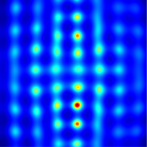
Finally, we study an irregular, complex case, for which the dynamics is always quasi-one-dimensional, since the solid blue Hopf bifurcation line lies underneath the black dashed line, below which we observe quasi-one-dimensional behaviour. An example of a simulation of (2.5) is shown in figure 9, where  $n=3$ and
 $m=1.3$ (black square), so according to (2.16), we are in the irregular regime. In figure 9(a) we show a perspective plot of
 $1/h$. While the peaks are smooth in the regular case, seen in figure 7(a), they are now broken up into many smaller peaks, producing a spatially ‘spotty’ behaviour. In the
 $y$-direction one observes the result of multiple instabilities, as seen in figure 3(b) for the one-dimensional case. In addition, as
 $x$ is detuned from
 $0.5$, this irregular behaviour is seen in different phases of its evolution, producing the hierarchy of peaks seen in figure 9. To emphasize the resulting complex spatial picture, in figure 9(b) we also represent
 $1/h$ as a colour contour plot in the plane.
Simulation of (2.5) with  $n=3,m=1.3$ (
 $\alpha \approx 0.63,\beta \approx 0.72$), and initial condition (3.1), using
 $\epsilon _1 = 0.05, \epsilon _2 = 0.03$ and
 $h_{ref}=0.1$. A quasi-one-dimensional, irregular singularity results, with periodic orbits. (a) A perspective plot of
 $1/h$ for
 $\tau =8.7$. Along the one-dimensional front, one observes a sequence of instabilities. (b) A contour plot of one of the peaks of
 $1/h$ (taken at the same time) shows the irregularity of the profile.

In figure 10 we test the expected form (2.31) more quantitatively. The one-dimensional periodic orbit, calculated from (2.12), was shown in figure 2(c,d). In our two-dimensional simulation  $h$ has been rescaled according to (1.1), in order to obtain the self-similar profile. In figure 10(a) we show the overall minimum of the profile, which should vary periodically, with period
 $T=3.7$. The theoretical prediction is shown as the blue curve in figure 10(a), which agrees very well with the numerical simulation for two periods. We attribute the deviation between theory and numerics for
 $\tau > 12$ to an eventual loss of resolution of the numerical code.
A quantitative test of (2.31), valid for the dynamical case. Parameters are the same as in figure 9, but two different values of  $h_{ref}$ are used. The one-dimensional, periodic profile is shown in figure 2(c). (a) We plot the minimum of
 $t'^{-\alpha }h$, along the centreline
 $y=0$ of the profile, compared with the theoretical prediction, with
 $T=3.7$. (b) The profile along the centreline is compared with the theoretical prediction. The profile taken at the minimum value of
 $H_{min}$ corresponds to
 $\tau = 9.2$, the profile at the maximum value of
 $H_{min}$ to
 $\tau = 9.9$.

To test the shape of the entire profile in its time evolution, we consider a cut through the profile at  $x=0.5$, rescaled according to (1.1). For simplicity, we record the shape of the profile when
 $H_{\min }$ is maximal and minimal, corresponding to the local maximum and minimum during the oscillation seen in figure 10(a). The profile from a full numerical simulation of (2.5) thus obtained (solid lines), is compared with the theoretical profiles in figure 10(b); very good agreement is found.
5. Discussion
In this paper we have pointed out generic structures of singularities in more than one dimension. The flexibility of the generalized thin film equation is useful to test many different scenarios using just one equation, but the features of higher-dimensional singularities we observed here carries over to many other equations as well. As examples of other systems we have mentioned the porous medium equation, the eikonal equation and the compressible Euler system.
To clarify how our approach generalizes to dimensions higher than two, let us consider three dimensions  ${\boldsymbol {x}} = (x,y,z)$. As before, we take
 $x$ as the direction in which the highest gradients occur, and
 $y,z$ are the ‘transversal’ directions. Now the detuning of the singularity time (2.20) has the form
 \begin{equation} t_c = t_0 + a_1y^2 + a_2 z^2, \end{equation}
where  $a_1$ and
 $a_2$ are positive constants, making sure that
 $t_c\ge t_0$. The similarity form of quasi-one-dimensional solutions becomes
 \begin{equation} h(x,y,z,t) = t'^{\alpha} H\left(\frac{x'}{t'^{\beta}},\frac{y'}{t'^{1/2}}, \frac{z'}{t'^{1/2}}\right), \end{equation}
where  $H$ satisfies
 \begin{equation} -\alpha H + \beta\xi H_{\xi} + \frac{\eta}{2} H_{\eta} + \frac{\zeta}{2} H_{\zeta} = \text{RHS}(\xi). \end{equation}
Here  $\text {RHS}(\xi ) = -[H^n H_{\xi \xi \xi } + H^{n-m-1}H_{\xi }]_{\xi }$ in the case of the thin film equation, but this may stand for any one-dimensional similarity problem. Finally, the unfolded solution of (5.3) becomes
 \begin{equation} H(\xi,\eta,\zeta) = (1 + A_1\eta^2 + A_2\zeta^2)^{\alpha} H^{(1)}\left(\frac{\xi + B\eta^{2\beta}} {\left(1 + A_1\eta^2 + A_2\zeta^2\right)^{\beta}}\right), \end{equation}
which generalizes (2.24).
When the interaction exponent  $m$ is large, interactions are very localized, and rupture occurs in a localized or ‘pointlike’ fashion, as had been observed previously. More complicated dynamics occurs if the interaction becomes more long-ranged, as
 $m$ becomes smaller. First, the higher-dimensional dynamics becomes an unfolding of one-dimensional dynamics, making it a superposition showing the singularity in all its phases. Second, the underlying one-dimensional singularity may become irregular, producing new structures as smaller and smaller scales are reached.
The combination of both effects may contribute to the understanding of turbulent fields, which are characterized by complexity both in scale and in space. As an illustration, in figure 11 we show a snapshot of  $1/h$ for a simulation of (2.5) with
 $n=3,m=1$ (black square in the phase diagram of figure 6), similar to that shown in figure 9. In that case, the one-dimensional dynamics is no longer merely periodic, but new structures keep being generated as one evolves toward smaller scales. Owing to the mechanism of unfolding, these new structures are translated into space, producing a spatially complex picture. As a result, one obtains a much more fractured picture than in the periodic case. This is clear especially in figure 11(b), where a contour plot of
 $1/h$ reveals a spatially complex pattern.


The non-periodic nature of the singularity also implies a sensitive dependence on initial conditions, as illustrated in figure 12. We show a larger spatial region, which encompasses more than six wavelengths  $\lambda _R = 0.44$ (see (2.7)) of the most unstable or Rayleigh mode of the initial film. As seen in figure 12(a), the film is perturbed slightly on the scale of the entire domain, producing a non-uniform picture of decay; the initial condition is seen to have a fourfold symmetry. We use the Basilisk version of our code, owing to its capabilities of automatic refinement.
Simulation of (2.5) with  $n=3,m=1$ in a large domain
 $[0,3]\times [0,3]$, using Basilisk. The code which produced the figure is available at http://basilisk.fr/sandbox/lopez/layer.c. (a) The initial condition
 $h_0(x,y) = 0.05[1 - 0.05\cos 2{\rm \pi} (x/3-1/2)] [1 - 0.03\cos 2{\rm \pi} (y/3-1/2)]$, as a colour plot of
 $1/h$. (b) A colour plot of
 $1/h$ for
 $h_{min} = 1.2 \times 10^{-2}$. Dark red corresponds to the smallest
 $h$, blue to the initial height. (c) The grid generated by Basilisk, with blue corresponding to level 7 (
 $\varDelta = 3/2^7 = 2.34 \times 10^{-2})$ and dark red to level 12 (
 $\varDelta = 3/2^{12} = 7.32 \times 10^{-4})$. A movie of the full evolution is available as supplementary movie 1 available at https://doi.org/10.1017/jfm.2021.286.

Since the evolution depends sensitively on the initial condition, slight changes in the initial condition translate into non-periodic behaviour on the small scale. In the final image, the local singularity is seen in many different stages of its evolution, producing a very non-uniform picture (figure 12(b) where  $h_{min} = 1.2 \times 10^{-2}$). Owing to small differences in how the refined grid is generated (see the image in figure 12(c)), the fourfold symmetry of the initial condition is broken, and each local singularity looks different. We confirmed that a different choice of parameters for grid refinement leads to a qualitatively similar result, but with a different pattern of broken symmetry. We conjecture that the square pattern of rupture points is a result of the square grid used by Basilisk. We have also performed simulations in a large domain for the parameters of figure 7, for which the dynamics is regular. No symmetry breaking was observed, as expected.
Although our simulation of the large domain in figure 12 does not have sufficient resolution, each local rupture point will have the intricately folded structure seen at a higher resolution in figure 11. Thus, non-periodic singular behaviour leads to a very intricate superposition of structure in space, but also in scale: upon a change of magnification, new patterns are seen.
Supporting data
Supporting data for this paper can accessed at https://zenodo.org/record/4506450#.YB0d5ejVuM9.
Supplementary movie
Supplementary movie is available at https://doi.org/10.1017/jfm.2021.286.
Acknowledgements
M.A.H. and J.M.L.-H. acknowledge financial support from the Ministerio de Economía y Competitividad and the Junta de Andalucia of the Kingdom of Spain under grants PID2019-108278-RB-C31 and P18-FR-3623, respectively.
Declaration of interests
The authors report no conflict of interest.
Appendix A. Similarity solutions and their stability
Here we apply the methods developed in Dallaston et al. (Reference Dallaston, Tseluiko, Zheng, Fontelos and Kalliadasis2017, Reference Dallaston, Fontelos, Tseluiko and Kalliadasis2018) to a range of  $n$-values. Going beyond the original papers, we use a new method to compute periodic solutions directly, and find a novel branch of asymmetric solutions. The computations are performed in the numerical continuation software AUTO07-P.
We implement our search for solutions using two different approaches. In the first method, used in Dallaston et al. (Reference Dallaston, Fontelos, Tseluiko and Kalliadasis2018, Reference Dallaston, Tseluiko, Zheng, Fontelos and Kalliadasis2017), we solve the linearized problem. We code explicitly the fourth-order ordinary differential equation (ODE) (2.10) for the similarity profiles, as well as the ODE for the eigenfunctions, as a system of first-order ODEs. This method is highly accurate and efficient, as AUTO's accurate collocation method is used to compute the derivatives in  $\xi$.
In the second method we solve the nonlinear dynamical equation (2.12) in scaled form. It is discretised in  $\xi$ using finite differences, and coded into AUTO. This method is advantageous in that we now compute stability in a natural way from the Jacobian of the system, and can explicitly compute branches of periodic (i.e. discrete self-similar) solutions. However, it is not as efficient, as AUTO is not designed to exploit the sparse/banded Jacobian structure that arises in discretised PDEs, and we have not been able to explore the complete structure of periodic solution branches.
A.1. Computation of solution branches by numerical continuation
In order to find and to continue off the pitchfork bifurcation discussed in § 2.3, a symmetry breaking term must be introduced into the equation for the similarity profile (2.10). Rearranging (2.10) for the fourth derivative, we obtain
 \begin{align} H^\textrm{(iv)} = H^{{-}n}(\alpha H - \beta\xi H') \!-\! n H^{{-}1}H'H''' - H^{{-}m-1}H'' \!-\! (n-m-1) H^{{-}m-2}H'^2 \!+\! \delta \xi\mathrm e^{-\xi^2}, \end{align}
where  $\delta$ is the strength of the added symmetry breaking term. Note that this term will not affect the boundary conditions, and if we reduce
 $\delta$ to zero, we obtain a solution to the original equation (2.10).
To find the first two branches  $H_0$ and
 $H_1$ of symmetric solutions, we set
 $\delta = 0$, and use the first method, starting from the known van der Waals solution at
 $n=3, m =3$ (Witelski & Bernoff Reference Witelski and Bernoff1999; Zhang & Lister Reference Zhang and Lister1999a). While a number of methods of computing the profile for these parameter values have been developed (Witelski & Bernoff Reference Witelski and Bernoff1999; Zhang & Lister Reference Zhang and Lister1999a; Tseluiko et al. Reference Tseluiko, Baxter and Thiele2013), we obtain it by computing a solution to the scaled time-dependent problem (2.12) until it reaches steady state, using the method described in Dallaston et al. (Reference Dallaston, Fontelos, Tseluiko and Kalliadasis2018). This branch (shown in black in figure 13(a,b)) is continued by varying
 $m$, until it reaches a turning point which represents the annihilation of this branch of solutions with another symmetric branch at a fold bifurcation (Dallaston et al. Reference Dallaston, Fontelos, Tseluiko and Kalliadasis2018, Reference Dallaston, Tseluiko, Zheng, Fontelos and Kalliadasis2017), marked by a square. These branches are then continued to all
 $1 \le n \le 3$. The cases
 $n=3$ and
 $n=1.5$ are shown in figures 13(a) and 13(b), respectively. By varying
 $m$, the fold bifurcation traces out a line in the
 $(m,n)$-plane, shown as the purple dash–dotted line in figure 14.
Solution branches for  $n= 3$ (a) and
 $1.5$ (b), represented by the minimum value
 $H_{min}$ of the similarity profile, as a function of
 $m$. Branches
 $H_0$ and
 $H_1$ are joined at a fold bifurcation. Periodic branches are born at the symmetric and antisymmetric Hopf bifurcations, an unstable asymmetric branch originates from a pitchfork bifurcation. In the lower panes (c,d), the real part of the largest non-trivial eigenvalue
 $\nu _R$ is shown along the asymmetric branch, as a function of
 $m$. For
 $n = 1.5$, a Hopf bifurcation is observed on the asymmetric branch (red circle), leading to stable, asymmetric similarity solutions for values of
 $m$ less than this point.

Location of all bifurcations detected in the  $(n,m)$-plane. At
 $n\approx 1.54$, the antisymmetric Hopf bifurcation and the pitchfork bifurcation collide.

In order to find asymmetric solutions, the symmetry breaking term is turned on by increasing  $\delta$ to a positive value. When
 $m$ is decreased, the
 $H_0$ solution branch passes through a pitchfork bifurcation (green crosses), at which an asymmetric branch originates, which consists of pairs of solutions, one a mirror image of the other. Once on the asymmetric branch,
 $\delta$ can be taken to zero again, and the solution branch is traced out by varying
 $m$, shown as the green dashed line in figure 13(a,b). This can once more be continued to all
 $1 \le n \le 3$, exhibiting the same structure; the pitchfork bifurcation is shown as the green dashed line in figure 14.
A.2. Stability and Hopf Bifurcations
Using the first method, the stability of similarity solutions is determined by solving the coupled system of equations for the eigenfunctions, as well as for the similarity profiles. The real and imaginary parts of the eigenvalue are used as continuation parameters. This approach was performed in Dallaston et al. (Reference Dallaston, Fontelos, Tseluiko and Kalliadasis2018), where the Hopf bifurcations that lead to discrete self-similarity were computed. For sufficiently large  $n$, there are two Hopf bifurcations on the ground state
 $H_0$, as seen in figure 13(a,b): as
 $m$ is decreased, the ground state solution is stable until the largest eigenvalue becomes positive at the ‘symmetric’ Hopf bifurcation (blue star), with the eigenfunction satisfying
 $P(-\xi ) = \overline {P(\xi )}$. As
 $m$ is decreased further, there is an ‘antisymmetric’ Hopf bifurcation (red plus) with the eigenfunction satisfying
 $P(-\xi ) = -\overline {P(\xi )}$. The symmetric and antisymmetric Hopf bifurcation lines are shown in the
 $(n,m)$-plane in figure 14 in blue and red, respectively. The fold bifurcation, at which
 $H_0$ and
 $H_1$ annihilate, is marked by a square in figure 13(c,d).
As  $n$ decreases, the antisymmetric Hopf bifurcation collides with the pitchfork bifurcation at a critical value
 $n \approx 1.54$; see figure 14. As this value is approached, the imaginary part of the eigenvalue at the Hopf bifurcation goes to zero (see figure 15a); that is, the period goes to infinity. This behaviour indicates a codimension-2 Bogdanov–Takens bifurcation (Kuznetsov Reference Kuznetsov2013). This type of bifurcation has recently also been observed in fourth-order PDEs (Tseluiko et al. Reference Tseluiko, Alesemi, Lin and Thiele2020), although for steady states and not similarity solutions as is the case in this study.
(a) The imaginary part of the eigenvalue at the antisymmetric Hopf bifurcation. At a critical value  $n\approx 1.54$, this Hopf bifurcation collides with the pitchfork bifurcation (depicted in figure 14), and the eigenvalue goes to zero, indicating a Bogdanov–Takens bifurcation. (b) The imaginary part of the eigenvalue at the Hopf bifurcation on the asymmetric branch. As the eigenvalue becomes large, computation in this region becomes difficult and the precise bifurcation structure in this regime is unclear.

The pitchfork bifurcation, where the asymmetric branch originates (found using the symmetry breaking term), is marked by a cross. We also compute the complex eigenvalues of the asymmetric branch, the largest real part  $\nu _R$ of which is shown in figure 13(c) for
 $n=3$ and figure 13(d) for
 $n=1.5$. For
 $n=3$,
 $\nu _R$ always remains positive, making the corresponding asymmetric branch unstable. For
 $n=1.5$, on the other hand,
 $\nu _R$ passes through zero at
 $m \approx 0.26$ (orange circle), where another Hopf bifurcation occurs, which restabilises the asymmetric branch as
 $m$ decreases. By numerical continuation we trace out the location of this new Hopf bifurcation in the
 $(n,m)$-plane, thus finding a region in which stable asymmetric similarity solutions exist (orange dotted line in figure 14).
This curve has a turning point at  $n \lesssim 1.87$, which indicates the origin of these bifurcations is a double-Hopf bifurcation (Kuznetsov Reference Kuznetsov2013). As
 $m$ decreases beyond this turning point, the imaginary part of the eigenvalue grows large, as seen in figure 15(b). It is not clear if there is another bifurcation at this point, or if the limits of the numerical scheme prevent the curve from being computed further.
A.3. Computation of periodic orbits
Periodic branches may be computed by using the second method, that is, explicitly coding the finite-difference discretised version of the PDE. In this case we restrict ourselves to  ${n=3}$ and focus on the branch of solutions leading off the symmetric and antisymmetric Hopf bifurcations, as plotted in figure 13(a). Using 1241 points and a domain size of
 $L = 20$, the two Hopf bifurcations on the ground state solution branch are found to good accuracy.
Continuing off the symmetric Hopf bifurcation (blue dot–dashed curve in figure 13(a)), periodic orbits remain symmetric for all scaled time  $\tau$;
 $H(\xi ,\tau ) = H(-\xi ,\tau )$. The value of
 $m$ increases from the bifurcation, into the region in which the steady symmetric solution is stable; this suggests the symmetric Hopf bifurcation is subcritical, and the symmetric periodic orbits are unstable, and indeed we have not observed any stable symmetric periodic orbits in full numerical simulations.
Continuing off the antisymmetric Hopf bifurcation (red dot–dashed curve in figure 13(a)), periodic orbits are computed for values of m decreasing from the bifurcation, past the point at which the steady solutions annihilate via the fold bifurcation. On this branch, similarity solutions have the mirror image property  $H(\xi , \tau ) = H(-\xi , \tau + T/2)$ as depicted for
 $n=3, m=1.3$ in figure 2(c). In principle the antisymmetric periodic branch should also be unstable close to the bifurcation, as the steady solution from which the branch bifurcates has already been destabilized by the symmetric Hopf bifurcation. However, full numerical simulations, as depicted in figure 10, indicate that the branch is an attractor sufficiently far from the bifurcation. The exact nature of the dynamics and exchange of stabilities in the region near the bifurcation pair requires further careful study beyond the scope of this article.
More generally, the solution profiles become more extreme in their asymmetry as  $n$ becomes small, and the numerical computation becomes less reliable, due to the errors both in discretisation and truncation (that is, applying the far-field boundary conditions at a finite distance from the origin). We use the numerical computation of the trivial eigenvalues
 $\nu _T,\nu _X$ as a check on the accuracy of the numerics, which becomes increasingly sensitive for the highly asymmetric solutions. All solution branches here are terminated when
 $\nu _T$ is more than
 $0.01$ different from the expected value of unity. There is clear scope, beyond this study, for carefully developing numerical tools that can be extended reliably to the more extreme regions of
 $(n,m)$ parameter space, to build a complete picture of the bifurcation structure of similarity solutions to (2.3).



