1 Introduction
For a variety of technological fluid and gas dynamics applications it is necessary to be able to control the boundary layer state. In particular, it is desirable to delay, or sometimes accelerate, a boundary layer laminar–turbulent transition. Gas suction from the boundary layer through a permeable surface is one such method to influence the position of the transition. Experiments show that using suction through a porous surface, it is possible to delay the onset of turbulence in the boundary layer and shift the position of the laminar–turbulent transition in the downstream direction. At subsonic flow velocities, critical Reynolds numbers of approximately
 $Re_{c}=40\times 10^{6}$
have been experimentally obtained. Nowadays, a large number of theoretical studies are available that attribute the stabilizing action of suction to the reduced thickness of the boundary layer and to the formation of a more preferable (in relation to hydrodynamic stability) velocity profile.
Thus, both experimental and theoretical data point to the possibility of stabilizing the boundary layer by suction. Detailed information on flow stabilization at subsonic and supersonic velocities can be found in the monographs by Gaponov & Maslov (Reference Gaponov and Maslov1980) and Boiko, Grek & Dovgal (Reference Boiko, Grek, Dovgal and Kozlov2006), and in many other sources. The majority of theoretical studies of boundary layer stabilization by suction disregard the properties of the permeable surface itself, but these may have a profound influence on the stability. The influence of the properties of the permeable coating on the stability of a subsonic boundary layer was theoretically examined for the first time by Gaponov (Reference Gaponov1971). In subsequent publications, this author developed the impedance relation between perturbations of the normal velocity and pressure at a permeable surface taking into consideration the effects of the compressibility of the gas. This relation was used to study both subsonic (Gaponov Reference Gaponov1975) and low supersonic flows (Gaponov Reference Gaponov1977). Later, Gaponov & Terekhova (Reference Gaponov and Terekhova2011, Reference Gaponov and Terekhova2013) investigated the interaction of disturbances in the boundary layers on impermeable surfaces in the presence of heat transfer and distributed mass transfer through a porous wall.
The cited papers dealt only with the theory, while experimental studies of the problem have been absent from the literature throughout the world for a long time. This can be best explained by the absence of a high-quality material for permeable coating at that time. However, recently the situation has changed. In recent years, experiments on the stability of hypersonic boundary layers have been performed (Fomin et al. Reference Fomin, Fedorov, Shiplyuk, Maslov, Burov and Malmuth2002, Reference Fomin, Fedorov, Kozlov, Shiplyuk, Maslov, Burov and Malmuth2004; Rasheed et al. Reference Rasheed, Hornung, Fedorov and Malmuth2002; Chokani et al. Reference Chokani, Bountin, Shiplyuk and Maslov2005). Their results are in satisfactory agreement with calculations (Fedorov et al. Reference Fedorov, Malmuth, Rasheed and Hornung2001, Reference Fedorov, Shiplyuk, Maslov, Burov and Malmuth2003) based on the approach suggested by Gaponov (Reference Gaponov1975, Reference Gaponov1977).
At supersonic speeds, the application of a permeable coating accelerates the transition, in contrast to a hypersonic boundary layer, where porosity delays the transition. This difference is related to the fact that the transition at supersonic velocities is defined by the first instability mode, whereas at hypersonic velocities the second instability mode plays an important role in the transition. An investigation of the first mode is more complicated because instability with respect to this mode is determined by oblique (three-dimensional, 3D) waves, whereas instability related to the second mode is determined by two-dimensional waves.
Unfortunately, porous coatings are rough in nature. For this reason, their effect on the transition is due to both permeability (unsteady gas flow inside the porous coating) and roughness. For example, to establish the effect of permeability (in particular, that of the thickness of the porous coating), it is desirable to conduct experiments with porous coatings at the same surface roughness (ideally, with the same internal structure). Then, at the same surface roughness, the development of the disturbance within the boundary layer and the transition Reynolds number ought to depend on the thickness of the porous coating.
This paper presents a theoretical and experimental study of the influence of the porosity and the roughness of a coating on the stability and laminar–turbulent transition of a supersonic boundary layer at Mach number
 $M_{\infty }=2$
. The purpose of this study is to investigate the combined influence of the permeability and roughness of the coating. For the first time at this Mach number, the development of disturbances artificially introduced in the boundary layer on such surfaces has been experimentally examined. A direct comparison of the measured and computed amplification curves and the spatial amplification rates is given.
2 Experimental set-up
The experiments were carried out in wind tunnel T-325 of the Institute of Theoretical and Applied Mechanics of the Russian Academy of Sciences (Bagaev, Lebiga & Pridanov Reference Bagaev, Lebiga, Pridanov and Chernykh1972) at a free-stream Mach number of
 $M_{\infty }=2$
, a stagnation temperature of
 $T_{0}\approx 290$
K and various values of the unit Reynolds number:
 $Re_{1\infty }=11\times 10^{6}~\text{m}^{-1}$
(transition investigations),
 $6.6\times 10^{6}~\text{m}^{-1}$
(measurements with natural disturbances) and
 $5\times 10^{6}~\text{m}^{-1}$
(measurements with controlled disturbances). Since this was a continuously running tunnel, the thermal boundary condition at the model surface during a typical experimental run (
 ${\sim}$
40 min) corresponded to an insulated wall. This means that the wall temperature was equal to the recovery temperature, and for selected
 $M_{\infty }$
and
 $T_{0}$
it was slightly below the ambient temperature:
 $T_{wall}\approx 273$
K.
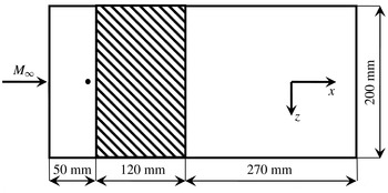
The scheme of the experimental flat-plate model, in plan view. The porous/rough insert is shown as a shaded region. The position of the source of artificial disturbances is shown by the small circle;
 $x_{source}=37$
mm.

The model was a stainless-steel flat plate 440 mm long, 10 mm thick and 200 mm wide, with a skew nose bevelled at an angle of
 $14^{\circ }$
and with a sharp leading edge (of bluntness radius
 $r_{b}<0.05$
mm). The scheme of the model is given in figure 1. The origin of the streamwise coordinate
 $x$
to be used in the present study (in the free-stream direction) is at the leading edge of the model. Over the working-surface segment 50–170 mm (throughout the whole width of the plate) the plate was provided with a 4.3 mm deep slot used for the fixation of various replaceable insert plates of different porosities, thicknesses, pore sizes and roughnesses.
In addition to porous inserts, we used also inserts with specified roughnesses (inserts coated with sandpaper with various grain sizes) close to the grain size and roughness of the porous inserts used.
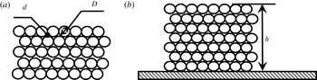
As the main purpose of this study was to investigate the combined influence of the permeability and roughness of the coating, we wanted to unite all inserts with porous and rough surfaces in a uniform set of the studied objects, for which it was necessary to unite them and systematize them at certain parameters, and first of all at an identical grain size and roughness. Naturally, there are some compromises in such an approach, but it was needed to compare the characteristics of the porous and rough inserts. In the present paper (for simplicity of comparison), we will consider the roughness surface as a thin permeable surface with porosity thickness equal to the thickness of the abrasive layer (approximately 1–2 grain diameters). Figure 2 shows the scheme of the porous and rough inserts (the grains are presented in the form of identical spheres).
Schematic representation of the porous and rough inserts: (a) planar view, (b) cross-section.

Seven inserts were used in the experiments: (1) a solid impermeable stainless-steel plate (insert 0); (2) a 39 % porosity plate manufactured of porous stainless-steel PNS-8 with
 $10~{\rm\mu}\text{m}$
filtration purity (analogous to the pore size) and 0.4 mm thickness (insert 2); (3) a 39 % porosity plate manufactured of porous stainless-steel PNS-8 with
 $10~{\rm\mu}\text{m}$
filtration purity and 2.5 mm thickness (insert 3); (4) a 32 % porosity plate manufactured of porous titanium TPP-5-MP of
 $40~{\rm\mu}\text{m}$
filtration purity and 2.5 mm thickness (insert 6); (5) impermeable insert 1 coated with sandpaper P220 having approximately the same grain size and roughness as for inserts 2 and 3 (grain size
 $D=70~{\rm\mu}\text{m}$
, roughness
 $R_{z}\approx 11~{\rm\mu}\text{m}$
); (6) non-porous insert 5 coated with sandpaper P60 with a grain size and roughness similar to that of insert 6 (
 $D=270~{\rm\mu}\text{m}$
,
 $R_{z}\approx 40~{\rm\mu}\text{m}$
); (7) non-porous insert 4 coated with sandpaper P120 with roughness
 $R_{z}\approx 18~{\rm\mu}\text{m}$
. Inserts 2, 3 and 6 were manufactured of a porous material commercially available from the Vyksa Metallurgical Plant and produced by the rolling and sintering of metal powders of various grain sizes. The parameters of all inserts used in the measurements are given in table 1.
Insert parameters.

It should be mentioned that we used inserts made of penetrable porous material of finite thickness. However, below the porous insert there was a stainless steel impermeable substrate. This means that there was no mean transpiration flow through the inserts. Only the fluctuation pressure fields penetrated the pores and underwent a viscous damping within the porous channels. Therefore, in our measurements we have investigated only the influence of porosity and roughness on the boundary layer stability, with zero mean flow through the surface under study.
The plate under study was fixed rigidly to the sidewalls of the test section of the wind tunnel at zero angle of attack. Artificial disturbances were introduced into the model boundary layer by means of a point glow discharge disturbance generator (Kosinov, Semionov & Shevelkov Reference Kosinov, Semionov and Shevelkov1994; Lysenko Reference Lysenko1999). The position of the boundary layer transition and its stability to natural and controlled disturbances were measured by a constant-resistance hot-wire anemometer operated with a single-wire sensor made of
 $10~{\rm\mu}\text{m}$
diameter tungsten wire 1.5 mm long. The overheat ratio of the sensor was 0.8; therefore, it could be assumed that the probe was sensitive predominantly to mass-flux fluctuations. Measurements of the downstream disturbance amplification (and the laminar–turbulent transition location) were performed in the vicinity of the disturbance maximum across the boundary layer, at
 $E=\text{const.}$
(where
 $E$
is the mean diagonal voltage across the hot-wire bridge), i.e. along the line of constant value of the mass flux. Disturbance measurements were performed around the line (
 $z=0$
) corresponding to the model centreline, at
 $|z|\leqslant 15$
mm, which was far enough from the test section sidewalls (located at
 $|z|=100$
mm) to reduce a possible parasitic influence of the sidewalls.
The fluctuation and mean flow quantities were measured by means of the automated data collection system described in detail in Kosinov, Semionov & Ermolaev (Reference Kosinov, Semionov and Ermolaev1999b
) and Kosinov et al. (Reference Kosinov, Ermolaev, Nikolaev, Semionov and Semisynov2007). The fluctuation voltage from the hot-wire anemometer was registered in a computer by an analogue-to-digital converter with a sampling rate of 750 kHz. The length of realization was 65 536 points. The average anemometer voltage was measured by an Agilent 34401A voltmeter; this voltage was subsequently registered in the computer through the serial port. Indications of mean and fluctuation flow characteristics were taken generally through each 2 mm on the longitudinal coordinate
 $x$
. The amplitude–frequency spectrum
 $A(f,x)$
was computed by averaging the measured power spectra.
3 Linear stability theory
Calculations on the basis of linear stability theory (LST) were performed on the assumption of a perfect gas with constant values of the specific heat ratio
 ${\it\gamma}=1.4$
and Prandtl number
 $Pr=0.72$
. It was assumed that the viscosity
 ${\it\mu}$
is a function of the temperature only according to the Sutherland relation. Within the framework of the linear stability problem, we represent the flow field in the compressible boundary layer as a combination of a time-mean flow and a low-amplitude perturbation. The main flow is considered in the self-similar approximation (Hayes & Probstein Reference Hayes and Probstein1959). Equations for disturbances are derived (by linearization) from the gas flow equations for a viscous heat-conducting compressible gas (Navier–Stokes, continuity and energy equations). We represent the solution of the problem as a set of harmonic waves,
 $$\begin{eqnarray}\displaystyle q=A(x){\bf\phi}(y)\exp \left(\text{i}\int _{x_{0}}^{x}{\it\alpha}(x^{\prime })\,\text{d}x^{\prime }+\text{i}{\it\beta}z-\text{i}{\it\omega}t\right), & & \displaystyle\end{eqnarray}$$
where
 $(x,y,z)$
are streamwise, normal-to-surface and spanwise coordinates; the disturbance wavevector
 $\boldsymbol{k}=({\it\alpha},{\it\beta})$
is composed of the streamwise
 ${\it\alpha}$
and spanwise
 ${\it\beta}$
wavenumbers;
 ${\it\omega}=2{\rm\pi}f$
and
 $f$
is the frequency. All quantities are taken non-dimensional in the standard way, which means with respect to the laminar boundary layer Blasius length scale
 ${\it\delta}=\sqrt{U_{e}{\it\rho}_{e}x/{\it\mu}_{e}}$
, mean velocity
 $U_{e}$
and values of pressure, density, temperature and viscosity taken at the boundary layer outer edge:
 $P_{e}$
,
 ${\it\rho}_{e}$
,
 $T_{e}$
,
 ${\it\mu}_{e}$
. Then, for the sought vector
 ${\bf\phi}=(u,u^{\prime },v,p,{\it\theta},{\it\theta}^{\prime },w,w^{\prime })^{\text{T}}$
, composed of perturbations of the three components of velocity
 $(u,v,w)$
, pressure
 $p$
and temperature
 ${\it\theta}$
, and their derivatives with respect to the normal coordinate
 $y$
, we obtain a system of linear ordinary differential equations
 $$\begin{eqnarray}\frac{\text{d}{\bf\phi}}{\text{d}y}=L(U,T){\bf\phi}.\end{eqnarray}$$
The non-zero elements of the linear Lees–Lin operator
 $L$
are given in Zhigulev & Tumin (Reference Zhigulev and Tumin1987); they depend on the properties of the mean flow (through the surface-normal profiles of mean velocity and temperature
 $(U(y),T(y))$
and on the parameters of the wave such as frequency and wavenumbers. System (3.2) has to be solved under the following boundary conditions. Outside of the boundary layer, we have
 $$\begin{eqnarray}|{\bf\phi}|\rightarrow 0\quad (y\rightarrow \infty ).\end{eqnarray}$$
According to Gaponov (Reference Gaponov1975, Reference Gaponov1977), the conditions on the permeable surface are
 $$\begin{eqnarray}u(0)=w(0)={\it\theta}(0)=0,\quad v(0)=Kp(0),\end{eqnarray}$$
where the complex parameter
 $K$
is the acoustic admittance of the porous coating.
To investigate the spatial stability, we assume that the frequency and spanwise wavenumber are real quantities, while the streamwise wavenumber
 ${\it\alpha}$
is a complex number. Then,
 ${\it\alpha}={\it\alpha}_{r}+\text{i}{\it\alpha}_{i}$
can be found as an eigenvalue of the boundary-value problem (3.2)–(3.4), while the components of
 ${\bf\phi}$
will be obtained as the corresponding eigenfunctions. Here, waves with
 $-{\it\alpha}_{i}>0$
refer to unstable disturbances growing in the downstream direction, while waves with
 $-{\it\alpha}_{i}\leqslant 0$
are stable decaying with
 $x$
.
The magnitude and phase of
 $K$
depend on the properties of the porous coating and on the characteristics of the wave propagating in the boundary layer. In this section, we examine the stability of the boundary layer on a flat plate covered by a porous layer of thickness
 $h^{\ast }$
(here, the asterisk denotes a dimensional quantity, whereas all variables without asterisks are assumed to be non-dimensionalized using the corresponding parameters). We consider a porous coating in the form of a thin flat plate with cylindrical pores uniformly covering the surface of the model, having a constant radius
 $r^{\ast }$
and oriented normal to the surface. The pore radius and the pore-to-pore distance
 $s^{\ast }$
are assumed to be much smaller in comparison to the boundary layer thickness and therefore smaller than the typical instability wavelength.
For the determination of the admittance
 $K$
in the case of a compressible gas, Gaponov (Reference Gaponov1975) used the theory of sound propagation in long narrow channels, assuming also
 $r^{\ast }\ll h^{\ast }$
. In such a case, the propagation of an acoustic wave is governed by the propagation constant
 ${\it\Lambda}$
and the impedance
 $Z_{0}$
,
 $$\begin{eqnarray}\displaystyle {\it\Lambda}=\sqrt{Z_{1}Y_{1}},\quad Z_{0}=\sqrt{Z_{1}/Y_{1}}, & & \displaystyle\end{eqnarray}$$
 $$\begin{eqnarray}\displaystyle Z_{1}=\frac{\text{i}{\it\omega}}{T_{w}}\frac{J_{0}(\boldsymbol{k})}{J_{2}(\boldsymbol{k})},\quad Y_{1}=-\text{i}{\it\omega}M^{2}\left[{\it\gamma}+({\it\gamma}-1)\frac{J_{2}(\boldsymbol{k}\sqrt{Pr})}{J_{0}(\boldsymbol{k}\sqrt{Pr})}\right],\quad \boldsymbol{k}=r\sqrt{\frac{\text{i}{\it\omega}{\it\rho}_{w}}{{\it\mu}_{w}}Re},\qquad & & \displaystyle\end{eqnarray}$$
where
 $M$
is the Mach number at the boundary layer outer edge,
 ${\it\rho}$
is the gas density,
 $r=r^{\ast }/{\it\delta}$
is the pore radius non-dimensionalized by the Blasius length scale
 ${\it\delta}$
,
 $J_{0}$
and
 $J_{2}$
are the Bessel functions of the corresponding order, and the subscript
 $w$
denotes the value of a quantity at the wall. For blind pores, closed at their bottom (at
 $y^{\ast }=-h^{\ast }$
) by a solid wall, the admittance
 $K$
can be represented as
 $$\begin{eqnarray}K=\frac{n}{Z_{0}}\tanh ({\it\Lambda}h),\end{eqnarray}$$
where
 $n$
is a porosity that defines the surface area fraction occupied by the pores. One can see that the magnitude of the admittance
 $K$
(3.7), which will determine the stability properties of the boundary layer over the porous coating, is directly proportional to the porosity
 $n$
and depends also on the pore radius
 $r$
(3.6). In our measurements, we used porous inserts with similar values of porosity but with quite different pore sizes, see table 1. If the porous layer is sufficiently thick (
 ${\it\Lambda}h\gg 1$
) (which is often the case), then
 $$\begin{eqnarray}K=-\frac{n}{Z_{0}}.\end{eqnarray}$$
The derivation of (3.4)–(3.8) is described in more detail in Gaponov (Reference Gaponov1975, Reference Gaponov1977) and Gaponov & Smorodsky (Reference Gaponov and Smorodsky2009).
The stability calculations were performed numerically by integrating the boundary-value problem for the eigenvalues of (3.2)–(3.4) with regard to relation (3.7) or (3.8) using the orthonormalization method (Gaponov & Maslov Reference Gaponov and Maslov1980).
4 Results
4.1 Some preliminary theoretical information about Mach 2 porous-coating boundary layer stability
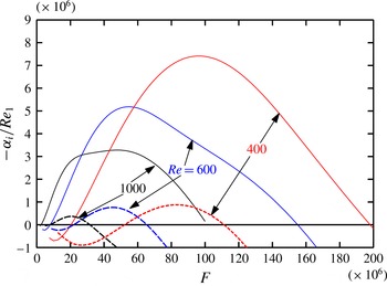
First, we discuss some basic theoretical results concerning the stability of a supersonic boundary layer on a porous surface. Figure 3 shows the spatial amplification rates
 $-{\it\alpha}_{i}$
of 2D instability waves versus the reduced frequency
 $F=2{\rm\pi}f{\it\mu}_{e}/{\it\rho}_{e}U_{e}^{2}$
for several values of the Reynolds number,
 $Re=400$
, 600, 1000. Computations were performed for deep pores
 $(h\rightarrow \infty )$
(3.8) with
 $r=0.5$
and
 $n=0.5$
. In this section all lengths have been made non-dimensional with respect to the Blasius boundary layer length scale
 ${\it\delta}=\sqrt{{\it\mu}_{e}x/U_{e}{\it\rho}_{e}}$
. Comparison of the growth rates computed for porous coatings (solid lines) and solid impermeable walls (dashed lines) reveals the possibility of a drastic destabilization of the boundary layer. The range of unstable frequencies is considerably enlarged, especially towards the region of higher frequencies, while the maximal amplification rates become three to eight times larger. Therefore, the application of the porous perforated coating at Mach number
 $M_{e}=2$
will only accelerate the laminar–turbulent transition.
Normalized spatial disturbance growth rate
 $-{\it\alpha}_{i}/Re_{1}$
versus reduced frequency
 $F$
for various Reynolds numbers:
 $Re=400$
, 600, 1000;
 $M_{\infty }=2$
,
 $r=0.5$
,
 $n=0.5$
,
 ${\it\Lambda}h\rightarrow \infty$
. The dashed lines are for a solid impermeable wall and the solid lines are for a surface with a porous coating.

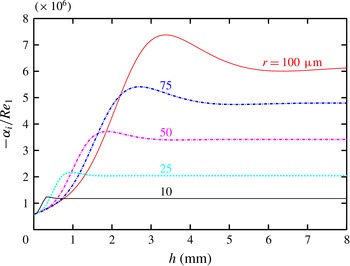
Figure 4 presents the amplification rates versus the dimensional value of the porous-coating thickness
 $h$
for
 $Re=600$
,
 $F=50\times 10^{-6}$
. These values correspond at the unit Reynolds number
 $Re_{1}=4\times 10^{6}~\text{m}^{-1}$
to a boundary layer thickness of
 ${\it\delta}_{BL}\approx 1$
mm for a wave with a frequency of
 $f=16$
kHz. One can see that an increase of the porous-coating thickness leads to an increase of the amplification rate, but this process is not monotonic: there is a certain value of
 $h$
where
 $-{\it\alpha}_{i}$
reaches its maximum. Further increase of
 $h$
will cause a certain reduction in
 $-{\it\alpha}_{i}$
and then the limiting case of deep pores (3.8) will be achieved. The thickness
 $h$
at which the limit is reached is dependent on the pore radius and becomes larger for larger pores. For example, for pores with
 $r^{\ast }=10~{\rm\mu}\text{m}$
, the thickness of the porous layer,
 $h\approx 0.5$
mm, could be considered as large, which ensures the applicability of equation (3.8).
Normalized spatial disturbance growth rate
 $-{\it\alpha}_{i}/Re_{1}$
versus porous-layer thickness
 $h$
at
 $M_{e}=2$
,
 $Re=600$
,
 $F=50\times 10^{-6}$
,
 $n=0.5$
for different values of the pore radius.

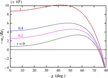
Figure 5 shows LST data on the influence of the pore radius on the growth rate of the unstable fluctuations in the supersonic
 $M=2$
boundary layer. The normalized spatial amplification rate
 $-{\it\alpha}_{i}^{\ast }{\it\delta}/Re_{1}$
of disturbances with the reduced frequency
 $F=50\times 10^{-6}$
, at a Reynolds number based on the Blasius length scale of
 $Re=U_{e}{\it\rho}_{e}{\it\delta}/{\it\mu}_{e}=600$
, is depicted as a function of the wavevector orientation angle
 ${\it\chi}=\arctan ({\it\beta}/{\it\alpha})$
for various values of the non-dimensional pore radius
 $0\leqslant r\leqslant 1$
(
 $r=r^{\ast }/{\it\delta}$
). One can see that a growth of
 $r$
leads to a monotonic increase of the wave amplification rate in the whole range of ‘unstable’ angles
 $0\leqslant {\it\chi}<75^{\circ }$
. In addition, the angle
 ${\it\chi}_{max}$
corresponding to the maximal growth rate
 $-{\it\alpha}_{i,max}=\max _{{\it\chi}}(-{\it\alpha}_{i})$
is shifted from
 ${\it\chi}_{max}\approx 58^{\circ }$
at
 $r=0$
to
 ${\it\chi}_{max}\approx 42^{\circ }$
at
 $r=1$
. However, the strongest influence of the porous coating on the amplification of perturbations occurs at small angles of orientation
 $0\leqslant {\it\chi}\leqslant 20^{\circ }$
. Therefore, the two-dimensional (2D,
 ${\it\chi}=0^{\circ }$
) perturbation at
 $r^{\ast }/{\it\delta}=1$
has an amplification rate almost an order of magnitude larger in comparison with the wave on the impermeable surface
 $(r=0)$
. Waves with higher inclination angles
 ${\it\chi}>70^{\circ }$
are much less influenced by the porosity: the variation in their growth rate with changing pore size is insignificant. Thus, according to LST, an increase of the pore radius destabilizes the supersonic boundary layer.
This is the specific character of the supersonic boundary layer in comparison with the hypersonic one, because experiments and computations (Fedorov et al.
Reference Fedorov, Malmuth, Rasheed and Hornung2001, Reference Fedorov, Shiplyuk, Maslov, Burov and Malmuth2003; Fomin et al.
Reference Fomin, Fedorov, Shiplyuk, Maslov, Burov and Malmuth2002, Reference Fomin, Fedorov, Kozlov, Shiplyuk, Maslov, Burov and Malmuth2004; Rasheed et al.
Reference Rasheed, Hornung, Fedorov and Malmuth2002; Chokani et al.
Reference Chokani, Bountin, Shiplyuk and Maslov2005) on hypersonic (
 $M\approx 6$
) boundary layer stability report a stabilizing influence of the porous coating on the second mode of instability, which plays the leading role in transition at this Mach number. However, in these experiments only the influence of porous coating on the amplification of 2D fluctuations has been investigated. Below we present a direct quantitative comparison of LST computations with experimental data for both 2D and 3D disturbances with
 ${\it\chi}\geqslant 0^{\circ }$
.
Normalized disturbance growth rate
 $-{\it\alpha}_{i}/Re_{1}$
versus wavevector orientation angle
 ${\it\chi}$
for various values of the non-dimensional pore radius
 $0\leqslant r^{\ast }/{\it\delta}\leqslant 1$
;
 $n=50\,\%$
,
 $F=50\times 10^{-6}$
,
 $Re=600$
.

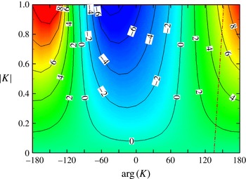
Contour plot of the non-dimensional spatial growth rate
 $-{\it\alpha}_{i}/Re_{1}\times 10^{6}$
on the plane
 $(|K|,\arg K)$
;
 $M_{e}=2$
,
 $Re=600$
,
 $F=50\times 10^{-6}$
,
 ${\it\chi}=0^{\circ }$
.

Until now, we have considered the influence on the boundary layer stability of a porous surface in the form of a perforated plate. Now, we briefly discuss a general porous layer which ensures the boundary conditions (3.4) but which is not limited to the specific particular case of a perforated plate. For our qualitative discussion, an arbitrary value, which is not determined by (3.7), will be given to the admittance
 $K$
.
Figure 6 shows an example of a contour plot of the spatial amplification rate on the plane ‘absolute value of the wall admittance
 $|K|$
–phase of admittance
 $\arg K$
’. Computations were performed for a wave of
 $F=50\times 10^{-6}$
,
 ${\it\chi}=0^{\circ }$
propagating in the boundary layer at
 $M_{e}=2$
,
 $Re=600$
.
Figure 6 demonstrates a principal possibility of stabilization influence of a porous coating on a supersonic boundary layer. Indeed, one can see that in fact the character of the influence of the porous coating is determined mostly by the phase shift between the normal velocity and the pressure disturbances at the wall (3.4), which is determined by the argument of the admittance,
 $\arg K$
, and depends on this phase shift; such an influence can be either destabilizing
 $(90^{\circ }<|\arg K|<180^{\circ })$
or stabilizing
 $(-90^{\circ }<\arg K<90^{\circ })$
. The growth rate, in comparison to the non-permeable solid surface
 $|K|=0$
, increases with increasing
 $|K|$
, which can be achieved by increase of either the pore radius or the porosity coefficient
 $n$
, or both. A real perforated porosity, assumed in this paper until now, gives the phase shift
 $135^{\circ }<\arg K<150^{\circ }$
(shown by the dash-dotted line in figure 6) depending on
 $r$
, but this is located in the region of destabilization. However, if it were possible to fabricate a permeable coating that is able to support a phase shift
 $-90^{\circ }<\arg K<60^{\circ }$
, with optimal
 $\arg K\approx -30^{\circ }$
for a wave of that frequency, it would lead to a reduction of the disturbance growth rate and boundary layer stabilization.
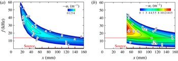
Stability diagram for inserts 0 (a) and 6 (b): dimensional (
 $\text{m}^{-1}$
) spatial amplification rate contours of 2D perturbations
 $-{\it\alpha}_{i}=-{\it\alpha}_{i}(x,f)~(\text{m}^{-1})$
,
 ${\it\chi}=0^{\circ }$
.

The phase shift responsible for boundary layer stabilization or destabilization is essentially dependent on the internal structure, i.e. the organization of the permeable coating. One example of a structure with a permeable surface has been investigated by Fomichev (Reference Fomichev1995), where flow stabilization was achieved at low subsonic velocities.
Linear stability of the supersonic boundary layer on a compliant surface has recently been investigated theoretically by one of the authors of the present paper (Gaponov Reference Gaponov2014). It was found that a flexible thin-film coating positioned above the porous perforated coating under certain conditions (in a certain frequency range in the region of high Reynolds numbers) can lead to a certain decrease of the spatial amplification rate of unstable disturbances, that is to a stabilization of the porous flat-plate boundary layer. This research was later expanded to the weakly nonlinear stage of disturbance development by Gaponov & Terekhova (Reference Gaponov and Terekhova2014). They found that not only is the linear disturbance growth rate reduced by the application of a compliant coating together with a porous surface, but also nonlinear interactions become weaker.
The stability diagram of the model boundary layer on the solid impermeable insert 0 for the conditions of the real experiment is presented in figure 7(a) by the contours of the dimensional spatial amplification rate for 2D waves on the plane ‘streamwise coordinate
 $x$
(mm)–frequency
 $f$
(kHz)’:
 $-{\it\alpha}_{i}=-{\it\alpha}_{i}(x,f)$
. The colour flooded area corresponds to the linear instability region where fluctuations are amplifying downstream:
 $-{\it\alpha}_{i}>0$
. The unstable region is separated from the area where perturbations decay with increasing streamwise coordinate by the neutral stability curve:
 ${\it\alpha}_{i}=0$
. The position of the solid and permeable inserts is sketched by the black horizontal strip, while the location of the disturbance generator is depicted by a small red square (‘Source’). Measurements of the disturbance amplitude were performed in the boundary layer above the inserts by a hot-wire probe at seven streamwise stations (
 $x=50$
, 65, 80, 95, 110, 125, 140 mm), as shown in figure 7(a) by red vertical rectangles. The
 ${\it\beta}$
-spectrum of the initial disturbance in terms of the excitation frequency was measured at
 $x=50$
mm. The computed stability diagram gives an idea of the unstable frequency range under the conditions of real experiments. In particular, one can see that in the middle of the measurement range (
 $x=95$
mm), the maximal amplification for 2D disturbances is at
 $f=14$
kHz (red solid horizontal line).
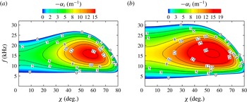
The stability diagram for three-dimensional (3D) disturbances computed for the middle measurement station (
 $x=95$
mm) is shown in figure 8(a). The spatial amplification rate contours are shown on the plane ‘wavevector orientation angle
 ${\it\chi}$
–frequency
 $f$
’:
 $-{\it\alpha}_{i}=-{\it\alpha}_{i}({\it\chi},f)$
. One can see that under the conditions of our measurements with impermeable insert 0, according to LST the most unstable 3D perturbations are waves with
 $f\approx 14$
kHz and
 ${\it\chi}\approx 60^{\circ }$
(red colour region). The amplification rate of such disturbances is approximately five times larger in comparison to 2D perturbations. Therefore, on the basis of the theoretical data presented in figures 7(a) and 8(a), we have chosen
 $f=14$
kHz for the disturbances, with the maximal amplification rate as a base frequency for the generation of the artificial disturbances in our experiments.
Figures 7(b) and 8(b) show stability diagrams, similar to those depicted in figures 7(a) and 8(a), but computed for porous insert 6 with the parameters
 $n=32\,\%$
,
 $2r^{\ast }=60~{\rm\mu}\text{m}$
. Linear stability theory calculations of the local growth rate (figure 7
b) were performed for the position of the porous insert only (
 $x>50$
mm). For the solid nose of the model (
 $x\leqslant 50$
mm), the stability diagram stays the same, like in figure 7(a). The instability region on the permeable coating, shown by the contours of
 $-{\it\alpha}_{i}=-{\it\alpha}_{i}(x,f)$
in figure 7(b), is wider in frequency in comparison with the similar region on the solid surface (figure 7
a).
Spatial amplification rate contours of 3D perturbations for inserts 0 (a) and 6 (b):
 $-{\it\alpha}_{i}=-{\it\alpha}_{i}({\it\chi},f)~(\text{m}^{-1})$
,
 $x=95$
mm.

Measured disturbance spectra: normalized r.m.s. fluctuation amplitude
 $A_{f{\it\beta}}$
versus spanwise wavenumber
 ${\it\beta}$
at various streamwise stations
 $50\leqslant x\leqslant 140$
mm for inserts 0, 3, 6 (a–c, respectively);
 $Re_{1\infty }=5\times 10^{6}~\text{m}^{-1}$
,
 $f=14~$
kHz.

Figure 8(b) presents the stability diagram
 $-{\it\alpha}_{i}=-{\it\alpha}_{i}({\it\chi},f)$
at
 $x=95$
mm computed for the porous coating. Comparison of figures 8(a) and 8(b) shows that the use of the porous coating leads to a slight increase of the unstable frequency range from
 $7\leqslant f\leqslant 27$
kHz on the solid surface to
 $4\leqslant f\leqslant 30$
kHz on the porous coating. The maximal growth rate of 3D perturbations increases from the value
 $-{\it\alpha}_{i,max}=\max _{f,{\it\chi}}[-{\it\alpha}_{i}(f,{\it\chi})]=15.8~\text{m}^{-1}$
(figure 8
a) to
 $-{\it\alpha}_{i,max}=19.7~\text{m}^{-1}$
(figure 8
b). However, the maximal growth rate of 2D perturbations increases from
 $-{\it\alpha}_{i,max}=\max _{f}[-{\it\alpha}_{i}(f,{\it\chi}=0)]\approx 3.3~\text{m}^{-1}$
on the impermeable surface to
 $-{\it\alpha}_{i,max}\approx 8.9~\text{m}^{-1}$
on the porous coating.
4.2 Influence of the pore size and the porosity thickness
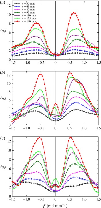
Theory needs some verification by experiment. To this end, we carried out measurements of the development of an artificial disturbance field, generated in the boundary layer by our source. Figure 9(a–c) shows the
 ${\it\beta}$
-spectra measured for the excitation frequency
 $f=14$
kHz in experiments with inserts 0, 3 and 6. The normalized root-mean-square (r.m.s.) fluctuation amplitudes
 $A_{f{\it\beta}}$
at selected measurement stations are shown versus the dimensional spanwise wavenumber
 ${\it\beta}$
 $\text{rad}~\text{mm}^{-1}$
. Comparison of figure 9(a–c) shows that in all three experiments with inserts 0, 3 and 6 the most amplifying disturbances in the downstream direction are fluctuations with
 ${\it\beta}=0.5{-}0.6~\text{rad}~\text{mm}^{-1}$
, while the amplification of disturbances on insert 6 is slightly higher than on inserts 0 and 3.
Normalized disturbance amplification curves for insert 6:
 $f=14$
kHz,
 ${\it\beta}=\pm 0.6~\text{rad}~\text{mm}^{-1}$
. Comparison of experiment (symbols) and LST (dashed lines):
 $2r^{\ast }=40$
, 60,
 $80~{\rm\mu}\text{m}$
(curves 1–3 respectively).

Figure 9(a) shows that for insert 0 the perturbations with
 ${\it\beta}=+0.6~\text{rad}~\text{mm}^{-1}$
are amplified by 7 times as
 $x$
increases from 50 to 140 mm, while disturbances with
 ${\it\beta}=-0.6~\text{rad}~\text{mm}^{-1}$
have grown only by 5.5 times. Thus, a certain asymmetry of the disturbance field is developing downstream. In measurements with the small pore size insert 3 (figure 9
b), not only are the 3D fluctuations with
 $|{\it\beta}|\approx 0.5~\text{rad}~\text{mm}^{-1}$
amplified, but there is also an anomalous growth of close-to-2D disturbances with
 $|{\it\beta}|<0.2~\text{rad}~\text{mm}^{-1}$
. In the experiments with the large pore size insert 6 (figure 9
c), the anomalous growth of 2D fluctuations is also visible but it is weaker in comparison with figure 9(b).
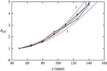
Figure 10 presents an example of a comparison of the computed (dashed lines) and measured (symbols) disturbance amplification data for insert 6 at
 $f=14$
kHz,
 ${\it\beta}=+0.6$
and
 $-0.6~\text{rad}~\text{mm}^{-1}$
(closed and open symbols respectively). The computations were performed not only for the nominal value of the pore size
 $2r^{\ast }=40~{\rm\mu}\text{m}$
given by the producer of the porous material but also for the values of 60 and
 $80~{\rm\mu}\text{m}$
. One can see that the best agreement of the computed amplification curve with the measured data can be obtained with the value of
 $2r^{\ast }=60~{\rm\mu}\text{m}$
, which is 50 % more than the filtration purity given by the producer. Similar computations were performed for various values of
 ${\it\beta}$
for both porous inserts 3 and 6. The conclusion drawn from this study is that for both porous inserts (with small and large pore size) the diameter of the pores used in LST computations should be taken to be 50 % more than the value of the filtration purity given by the producer. Only in this case is it possible to obtain good overall agreement of theory and measurements for the disturbance amplification curves. The explanation for this phenomenon could be given as follows. The filtration purity is determined by the maximal size of solid particles able to penetrate through the given sample of porous material. However, this does not correspond to the efficient pore size for the gas, but determines only a certain minimal pore size of the permeable material. For the theory used in this paper, we need the efficient pore diameter of the permeable coating, and this diameter was identified by the described comparison of the computations and the measured data. As the manufacturing technology of all porous inserts was identical, in the calculations the effective pore diameter was taken to be one and a half times more than the filtration purity size in all cases.
Spatial disturbance amplification rate
 $-{\it\alpha}_{i}$
versus spanwise wavenumber
 ${\it\beta}$
for inserts (0) solid; (3) porous,
 $d=10~{\rm\mu}\text{m}$
(
 $d=15~{\rm\mu}\text{m}$
, LST),
 $h=2.5$
mm; (6) porous,
 $d=40~{\rm\mu}\text{m}$
(
 $d=60~{\rm\mu}\text{m}$
, LST),
 $h=2.5$
mm;
 $f=14$
kHz,
 $Re_{1\infty }=5\times 10^{6}~\text{m}^{-1}$
,
 $x=95$
mm. Comparison of measurements (symbols) with the theory (solid lines).

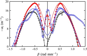
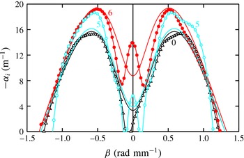
Figure 11 shows a direct comparison of the measured (symbols) and computed (solid lines) local spatial amplification rate
 $-{\it\alpha}_{i}=-{\it\alpha}_{i}({\it\beta})$
at
 $x=95$
mm. The experimental growth rates were determined by means of a polynomial regression of the measured data for growth curves
 $\ln A(x)$
of the disturbances with various values of
 ${\it\beta}$
. The amplification rate was then determined by the formula
 $-{\it\alpha}_{i}=\partial \ln A(x)/\partial x$
. The dimensional values of the amplification rate are shown in figure 11 versus the spanwise wavenumber. Linear stability theory computations were performed for various values of the pore diameter
 $2r^{\ast }$
. Once again, we get a result that the best agreement of the local LST growth rates with the measurements could be obtained for a pore diameter that is 50 % larger than the value of the filtration purity given by the producer. The solid lines in figure 11 represent the results of LST computations with these increased values of the pore diameter. One can see a good agreement of the computed (solid lines) and experimental (curves with symbols) amplification rates at
 $|{\it\beta}|\geqslant 0.25~\text{rad}~\text{mm}^{-1}$
. The increase of the pore diameter leads to an increase of the growth rate for all values of
 ${\it\beta}$
, but this influence is stronger at
 ${\it\beta}\approx 0$
, in agreement with the theoretical prediction (figure 5). The location of the maximal growth rate
 $-{\it\alpha}_{i,max}=\max _{{\it\beta}}[-{\it\alpha}_{i}({\it\beta})]$
computed for the conditions of the measurements is shifted from
 $|{\it\beta}|\approx 0.6~\text{rad}~\text{mm}^{-1}$
at
 $r=0$
(insert 0) to
 $|{\it\beta}|\approx 0.5~\text{rad}~\text{mm}^{-1}$
at
 $2r^{\ast }\approx 40~{\rm\mu}\text{m}$
(insert 6). One can see that the agreement of theory and experiment concerning the position of the maximal growth rate is good for inserts 0 and 6 (for insert 3 it is a little worse). The magnitude of the maximal experimental amplification rate
 $-{\it\alpha}_{i,max}$
also agrees well with the LST data. A disagreement between theory and measurement is observed for small values of
 $|{\it\beta}|<0.2~\text{rad}~\text{mm}^{-1}$
. In the experiment, a strong anomalous growth at
 ${\it\beta}$
close to zero occurs. The reason for this discrepancy is the beginning of nonlinear processes in the boundary layer (Kosinov, Ermolaev & Semionov Reference Kosinov, Ermolaev and Semionov1999a
; Terekhova Reference Terekhova2012).
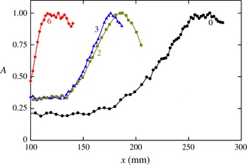
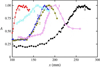
Next, the influence of the pore size on the boundary layer transition was investigated. Figure 12 shows the dependence of the dimensionless (normalized to unity at the maximum) r.m.s. hot-wire signal
 $A$
(integrated over the whole disturbance spectrum) on the longitudinal coordinate
 $x$
(measured from the leading edge along the model surface) at
 $Re_{1\infty }=11\times 10^{6}~\text{m}^{-1}$
for inserts 0, 3 and 6 (curves 0, 3 and 6 respectively). The interval
 ${\rm\Delta}x$
over which the amplitude of the integral fluctuations grows comprises a linear region and a nonlinear region of the laminar–turbulent transition in the model, while the maximum of each of the presented dependences refers to the position of the laminar–turbulent transition. Since the porosities of inserts 3 and 6 are approximately the same, it follows from figure 12 that with increasing pore radius, the position of the boundary layer transition moves towards the leading edge. Therefore, the porous coating accelerates the transition of the supersonic Mach 2 boundary layer, and we can regard the coating as exerting a destabilizing action.
Influence of the pore size and the porosity thickness on the transition position: (0) solid; (2)
 $d=10~{\rm\mu}\text{m}$
,
 $h=0.4$
mm; (3)
 $d=10~{\rm\mu}\text{m}$
,
 $h=2.5$
mm; (6)
 $d=40~{\rm\mu}\text{m}$
,
 $h=2.5$
mm.

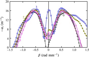
Then, the influence of the porosity thickness on the boundary layer stability and transition was investigated. In figure 13, the spatial disturbance amplification rate depending on the transverse wavenumber at
 $x=95$
mm for inserts 0, 2, 3 is shown. A comparison of experiments (symbols) with the theory (lines) was made.
It makes sense to carry out the comparison close to the maximum of the increment, i.e. in the place where the error of the experimental definition is minimal. In figure 13, in the vicinity of maxima of the amplification rate rather good quantitative agreement between theory and experiment is visible. It should be noted that even near the maxima of the measured disturbance spectra at the generator frequency, the amplitude of the mass-flux disturbances does not surpass 1 % of the average mass flux. In figure 13, it is possible to see also the beginning of the nonlinear processes occurring in the boundary layer. It is shown in the abnormal growth of quasi-two-dimensional waves with small values of the transverse wavenumber
 $|{\it\beta}|<0.1~\text{rad}~\text{mm}^{-1}$
. It is most pronounced on the thick porous insert 3. Despite the existence of a nonlinearity in the disturbance field, the development of the waves
 $|{\it\beta}|=0.5{-}0.7~\text{rad}~\text{mm}^{-1}$
, dominating in the
 ${\it\beta}$
-range, occurs in full agreement with linear stability theory.
Influence of the porosity thickness on the boundary layer stability: (0)
 $h=0$
mm; (2)
 $h=0.4$
mm; (3)
 $h=2.5$
mm;
 $f=14$
kHz,
 $Re_{1\infty }=5\times 10^{6}~\text{m}^{-1}$
,
 $x=95$
mm. Comparison of measurements (symbols) with theory (lines).

The experimental data on the effect of the thickness of the porous coating on the position of the transition are illustrated in figure 12. Here, the non-dimensionalized hot-wire r.m.s. value (versus the longitudinal coordinate) is shown for (a) porous insert 2 with
 $d=10~{\rm\mu}\text{m}$
and
 $h=0.4$
mm (curve 2), (b) porous insert 3 with
 $d=10~{\rm\mu}\text{m}$
and
 $h=2.5$
mm (curve 3). Inserts 2 and 3 had the same surface roughness but different pore depths. The interval
 ${\rm\Delta}x$
over which the integral over the spectrum pulsation amplitude shows a notable growth refers to the nonlinear region of disturbance growth in the boundary layer (i.e. to the transition boundary layer, which was previously laminar), and the maximum of each of the shown dependences refers to the position of the laminar–turbulent transition.
Since the roughness, porosity and pore size values of inserts 2 and 3 are the same, the data in figure 12 suggest that with decreasing porous-layer thickness the laminar–turbulent transition moves away from the leading edge of the model. At one and the same surface roughness value, the depth of the pores affects the transition.
Thus, the increase of the porous-coating thickness leads to a boundary layer destabilization that accelerates the laminar–turbulent transition.
4.3 Combined influence of the permeability and roughness
The joint effect of the permeability and the roughness on the boundary layer stability and transition was investigated. First, the boundary layer stability (for natural disturbances) was experimentally investigated with inserts 0–3 at
 $Re_{1\infty }=6.6\times 10^{6}~\text{m}^{-1}$
, and the obtained data were compared with the results of the LST calculations. The spanwise wavenumber
 ${\it\beta}$
selected in the calculations was such that the best agreement with the experimental data for the impermeable smooth plate was achieved. The calculations showed that at the adopted unit Reynolds number
 $Re_{1\infty }=6.6\times 10^{6}~\text{m}^{-1}$
the best agreement of the theoretical curves of the disturbance amplitude growth with the experimental data was obtained at
 ${\it\beta}=\text{const.}\approx 0.22~\text{rad}~\text{mm}^{-1}$
. This value of
 ${\it\beta}$
was used in the calculations of the disturbance amplitude growth curves for the plate with porous inserts.
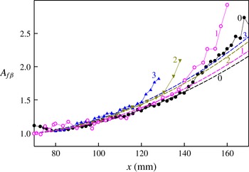
In figure 14, the disturbance amplitude growth curves, both experimental and calculated (
 ${\it\beta}=0.22~\text{rad}~\text{mm}^{-1}$
), are presented at the frequency
 $f=10$
kHz for inserts 0, 2 and 3, that is, with the non-porous smooth surface (0) and with porous (
 $d=10~{\rm\mu}\text{m}$
) inserts, 0.4 (2) and 2.5 mm (3) thick. To compare the disturbance amplification over various inserts, the presented growth curves were normalized by unity at the position
 $A|_{x=70~\text{mm}}=1$
. It is interesting to note that the experimental data for the rough insert 1 (
 $d=10~{\rm\mu}\text{m}$
,
 $h=0.1$
mm) are in agreement with the theoretical curve computed for the porous, 0.15 mm thick, insert at
 ${\it\beta}=0.22~\text{rad}~\text{mm}^{-1}$
(curve 1).
Good agreement between the calculated results and the experimental data can be seen. The deviation of the experimental curves from the linear theory indicates the onset of the nonlinear stage of the disturbance development, that is, the beginning of the laminar–turbulent transition of the boundary layer, which occurs on the impermeable smooth plate (0) at
 $x\approx 140$
mm, while on the model with the rough insert 1 it takes place at
 $x\approx 135$
mm, on the model with porous insert 2 at
 $x\approx 125$
–130 mm and on the model with the porous insert 3 at
 $x\approx 120$
mm. The earlier onset of the nonlinear stage on porous coatings, as compared with the rough non-porous plate, is due to the higher disturbance level in the boundary layer on the permeable surfaces. From figure 14 it also follows that on the thin (0.4 mm) porous insert 2 the stability is higher than on the thicker insert 3 (2.5 mm).
Disturbance amplification curves
 $A_{f}=A_{f}(x)$
at
 $f=10$
kHz,
 $Re_{1\infty }=6.6\times 10^{6}~\text{m}^{-1}$
,
 ${\it\beta}=0.22~\text{rad}~\text{mm}^{-1}$
. Comparison of computation (dashed lines) and experiment (solid lines with symbols), inserts 0–3.

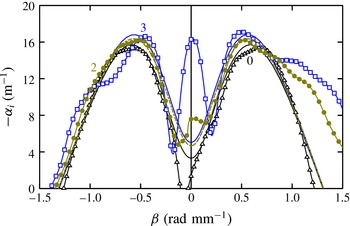
Then, the roughness influence on the boundary layer stability (for controlled disturbances) was investigated. Figure 15 shows the experimental disturbance spatial amplification rate as a function of the spanwise wavenumber for different inserts: (0) solid; (1) rough (coated with the abrasive paper P220),
 $D=70~{\rm\mu}\text{m}$
; (4) rough (coated with the abrasive paper P120),
 $D=125~{\rm\mu}\text{m}$
; (5) rough (coated with the abrasive paper P60),
 $D=270~{\rm\mu}\text{m}$
. As follows from figure 15, for a rough surface, as the coating roughness increases, the stability of the boundary layer decreases.
Influence of roughness on the stability of the boundary layer: (0)
 $R_{z}=0$
; (1)
 $R_{z}\approx 11{-}12~{\rm\mu}\text{m}$
; (4)
 $R_{z}\approx 18~{\rm\mu}\text{m}$
; (5)
 $R_{z}\approx 30~{\rm\mu}\text{m}$
;
 $f=14$
kHz,
 $Re_{1\infty }=5\times 10^{6}~\text{m}^{-1}$
,
 $x=95$
mm.

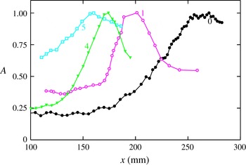
Influence of the coating roughness on the position of the transition: (0)
 $R_{z}=0$
; (1)
 $R_{z}\approx 11{-}12~{\rm\mu}\text{m}$
; (4)
 $R_{z}\approx 18~{\rm\mu}\text{m}$
; (5)
 $R_{z}\approx 30~{\rm\mu}\text{m}$
.

The results for the effect of the coating roughness on the transition position are shown in figure 16.
We will briefly dwell on the effect of the roughness size of the model surface on the position of the boundary layer transition. In such investigations, the critical Reynolds number
 $Re_{k}$
is usually determined based on the roughness size (
 $\boldsymbol{k}$
is the roughness element height), starting from which the roughness influences the transition position.
The roughness can be either isolated or distributed. Naturally,
 $Re_{k}$
is higher for isolated than for distributed roughness. For example, in the classic study of van Driest & McCauley (Reference van Driest and McCauley1960), where the effect of a transverse chain of isolated spherical roughness elements is described, it was obtained that
 $Re_{k}\approx 1500$
–1700 at
 $M_{e}=2.0{-}3.4$
.
For distributed roughness (precisely this roughness is used in our study),
 $Re_{k}$
is considerably smaller. In Braslow, Knox & Horton (Reference Braslow, Knox and Horton1959), the effect of distributed granular roughness (made of silicone carbide sand) on the transition on a flat plate was investigated. For
 $M_{e}\approx 2$
and a thermally insulated surface, it was found that
 $Re_{k}\leqslant 580$
. In Braslow & Horton (Reference Braslow and Horton1958), Braslow, Hicks & Harris (Reference Braslow, Hicks and Harris1966) and Jones (Reference Jones1959), the results of investigation of the effect of distributed granular roughness on the transition on 10 cones are presented. In an investigation by Braslow & Horton (Reference Braslow and Horton1958) for
 $M_{e}=1.6$
to 2,
 $Re_{k}=260$
–580 was obtained; in Braslow et al. (Reference Braslow, Hicks and Harris1966),
 $Re_{k}\approx 600$
for
 $M_{e}\leqslant 2$
; and in Jones (Reference Jones1959),
 $Re_{k}\approx 400$
for
 $M_{e}=4$
. Judging from the data of Braslow & Horton (Reference Braslow and Horton1958), Braslow et al. (Reference Braslow, Knox and Horton1959, Reference Braslow, Hicks and Harris1966) and Jones (Reference Jones1959), in our experiments with insert 1 (
 $Re_{k}\approx 800$
), the critical size of the roughness grain is exceeded only slightly.
According to Schneider (Reference Schneider2008), one of the main modes by which the roughness may affect the instability and transition is the following: free-stream disturbances such as acoustic waves may interact with the surface roughness to generate boundary layer disturbances such as first-mode or second-mode waves, which then are amplified and cause a transition downstream.
In figure 16, we have plotted the dependence of the dimensionless r.m.s. signal
 $A$
from the hot-wire anemometer probe on the longitudinal coordinate
 $x$
at
 $Re_{1\infty }=11\times 10^{6}~\text{m}^{-1}$
for the smooth (polished) insert 0 and the rough inserts 1, 4, 5. The Reynolds numbers based on the roughness grains of inserts 1, 4 and 5 are
 $Re_{k}\approx 800$
, 1400 and 2900.
As follows from figure 16, the boundary layer transition monotonically approaches the leading edge of the model as the model surface is successively changed as follows: (1) solid surface; (2) rough surface with
 $R_{z}\approx 11{-}12~{\rm\mu}\text{m}$
; (3) rough surface with
 $R_{z}\approx 18~{\rm\mu}\text{m}$
; (4) rough surface with
 $R_{z}\approx 30~{\rm\mu}\text{m}$
. Thus, for a rough surface, as the coating roughness increases, the boundary layer transition monotonically approaches the leading edge.
Figures 17 (for pore size
 $d=40~{\rm\mu}\text{m}$
) and 18 (for
 $d=10~{\rm\mu}\text{m}$
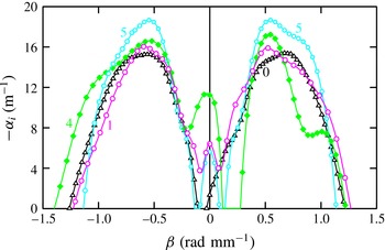
) show the joint effect of the permeability and roughness on the boundary layer stability. Figure 17 presents the disturbance spatial amplification rate versus the spanwise wavenumber for inserts 0, 5 and 6. Figure 18 gives analogous data for inserts 0 and 1–3.
Joint effect of roughness and permeability on the boundary layer stability for
 $d=40~{\rm\mu}\text{m}$
: (0) solid; (5) rough,
 $R_{z}\approx 30~{\rm\mu}\text{m}$
,
 $d=40~{\rm\mu}\text{m}$
,
 $h=0.2~\text{mm}$
; (6) porous,
 $R_{z}\approx 30~{\rm\mu}\text{m}$
,
 $d=40~{\rm\mu}\text{m}$
,
 $h=2.5$
mm;
 $f=14$
kHz,
 $Re_{1\infty }=5\times 10^{6}~\text{m}^{-1}$
,
 $x=95$
mm. Comparison of measurements (symbols) with LST (solid lines).

Joint effect of permeability and roughness on the boundary layer stability for
 $d=10~{\rm\mu}\text{m}$
: (0) solid; (1) rough,
 $R_{z}\approx 11{-}12~{\rm\mu}\text{m}$
,
 $d=10~{\rm\mu}\text{m}$
,
 $h=0.1$
mm; (2) porous,
 $R_{z}\approx 11{-}12~{\rm\mu}\text{m}$
,
 $d=10~{\rm\mu}\text{m}$
,
 $h=0.4$
mm; (3) porous,
 $R_{z}\approx 11{-}12~{\rm\mu}\text{m}$
,
 $d=10~{\rm\mu}\text{m}$
,
 $h=2.5~\text{mm}$
;
 $f=14$
kHz,
 $Re_{1\infty }=5\times 10^{6}~\text{m}^{-1}$
,
 $x=95$
mm. Comparison of measurements (symbols) with LST (solid lines).

Figures 17 and 18 show that for a rough and porous coating (of the same grain size and roughness), with an increase in the thickness of the coating, the boundary layer stability diminishes.
The experimentally obtained results on the joint effect of the coating roughness and porosity on the position of the transition are shown in figure 19. Here, we have plotted the dependence of the dimensionless r.m.s. signal
 $A$
from the hot-wire anemometer probe on the longitudinal coordinate
 $x$
at
 $Re_{1\infty }=11\times 10^{6}~\text{m}^{-1}$
for inserts 0–3 and 5–6.
Joint influence of the coating roughness and permeability on the position of the transition: (0) solid,
 $h=0$
; (1) rough,
 $R_{z}\approx 11{-}12~{\rm\mu}\text{m}$
,
 $d=10~{\rm\mu}\text{m}$
,
 $h=0.1$
mm; (2) porous,
 $R_{z}\approx 11{-}12~{\rm\mu}\text{m}$
,
 $d=10~{\rm\mu}\text{m}$
,
 $h=0.4$
mm; (3) porous,
 $R_{z}\approx 11{-}12~{\rm\mu}\text{m}$
,
 $d=10~{\rm\mu}\text{m}$
,
 $h=2.5$
mm; (5) rough,
 $R_{z}\approx 30~{\rm\mu}\text{m}$
,
 $d=40~{\rm\mu}\text{m}$
,
 $h=0.2$
mm; (6) porous,
 $R_{z}\approx 30~{\rm\mu}\text{m}$
,
 $d=40~{\rm\mu}\text{m}$
,
 $h=2.5$
mm.

As follows from figure 19, for the same grain size, either
 $D=70~{\rm\mu}\text{m}$
(
 $d=10~{\rm\mu}\text{m}$
) or
 $D=270~{\rm\mu}\text{m}$
(
 $d=40~{\rm\mu}\text{m}$
), the boundary layer transition monotonically approaches the leading edge of the model, as the model surface is successively changed as follows: (1) solid surface (
 $h=0$
); (2) rough surface (
 $h=0.1{-}0.2$
mm); (3) porous surface (
 $h=0.4$
mm); (4) porous surface (
 $h=2.5$
mm). This means that at the same roughness, the laminar–turbulent transition position approaches the leading edge of the model as the thickness of the porous layer increases.
Thus, the joint effect of the permeability and the roughness of the flat-plate surface on the boundary layer stability and laminar–turbulent transition has been experimentally and theoretically investigated at the free-stream Mach number
 $M_{\infty }=2$
. It has been shown that as a certain roughness value is reached, with an increase in the thickness of a rough and porous coating, there is less stability of the boundary layer, and the laminar–turbulent transition is displaced towards the leading edge of the model.
Therefore, the use of permeable coating at Mach 2 facilitates the onset of turbulence in the boundary layer. It looks disadvantageous because of the higher wall friction and wall heat transfer of the turbulent boundary layer. However, sometimes in order to control the flow around a flying vehicle in the conditions of real flight it is more preferable to maintain the boundary layer in a turbulent state despite its higher friction. Indeed, the laminar boundary layer is extremely sensitive to all possible external influences, while the turbulent one is much more tolerant to change of the external forcing. Moreover, the separation of a laminar boundary layer usually takes place earlier (further upstream) than that for the turbulent boundary layer under the same external conditions. Therefore, acceleration of a boundary layer transition by application of a thin porous coating may lead to a downstream shift of the separation region, thereby improving the flow around the body and reducing its total drag at moderate supersonic speeds. Moreover, flow turbulization is preferable in various technological processes, for example in chemistry, for intensification of mixing. In such cases, the turbulent boundary layer produced by porous coating has an advantage in relation to the laminar one. This is also true for scramjets, where the fuel is injected through the permeable walls and it is necessary to intensify the mixing and therefore combustion (Capra et al. Reference Capra, Boyce, Kuhn and Hald2015).
5 Basic conclusions
A combined theoretical and experimental investigation of the influence of the parameters of a porous and rough coating (pore size, porous-coating thickness and roughness) on the first-mode stability and the laminar–turbulent transition of a flat-plate supersonic boundary layer at the free-stream Mach number
 $M_{\infty }=2$
has been performed. Artificial disturbances have been introduced into the boundary layer of the model by means of a harmonic point glow discharge disturbance generator.
For various porous coatings, there is good quantitative agreement of the linear stability theory computations with the experiments carried out. The theoretical and experimental integral amplification curves and local spatial amplification rates correlate well. It has been shown that an increase of the pore size and the porous-coating thickness leads to a boundary layer destabilization that accelerates the laminar–turbulent transition. The results of these theoretical and experimental investigations qualitatively indicate that at supersonic speeds the stabilizing influence of suction on the boundary layer stability and transition can be jeopardized or overcome by the destabilizing influence of the permeable surface on the development of boundary layer unstable fluctuations.
In spite of the fact that for the real perforated porosity considered in this paper the permeability destabilizes the supersonic boundary layer, the possibility of a stabilizing influence of porosity on linear stability exists. It is only necessary to find some means to change the phase shift of the disturbance at the surface (perhaps, for example, by means of a thin compliant foil above the porous coating of finite thickness, or in other ways).
In the presented research on the combined effect of the model surface permeability and roughness on the boundary layer stability and transition, it has been shown that as a certain (critical) roughness value is reached, with an increase in the thickness of a rough and porous coating, the boundary layer stability diminishes and the laminar–turbulent transition is displaced towards the leading edge of the model.
Acknowledgements
This paper was partially supported by the Russian Foundation for Basic Research (project 15-01-00866-a) and the Russian Academy of Sciences (ITAM project 01201351885).