


1. Introduction
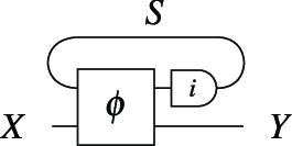
Many objects of study in computer science, such as Mealy machines, clocked digital circuits, signal flow graphs, discrete-time feedback loops, and recurrent neural networks (RNNs), compute a stateful and particularly a causal function on an infinite sequence of inputs. Here, “causal” means the output of the function at a particular index in the sequence may depend only on the inputs at that index and before.Footnote 1 These devices share a basic operational scheme, depicted in Figure 1.
Here the box labeled
 $\phi$
is a (sub)device which takes an
 $S$
-value at its upper left interface and an
 $X$
-value at its lower left interface and produces output
 $S$
- and
 $Y$
-values at its right interfaces. The differently shaped box labeled
 $i$
is our depiction of a delay gate, a device which stores the value provided to its left boundary and emits it one step later at its right boundary, initially emitting the value
 $i$
. The whole device, which we call
 $\Phi$
, receives sequences of
 $X$
-valued inputs at the left and emits sequences of
 $Y$
-valued outputs at the right, storing its internal state in the delay gate.
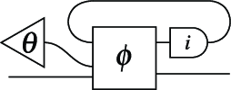
A RNN has inputs of two types: data inputs and parameters. Training a neural network means finding parameter values
 $\theta$
so that when
 $\theta$
is fixed (by the triangular device in Figure 2 which emits
 $\theta$
constantly), the resulting function of data inputs has a desired behavior.
A basic causal device.

A simple RNN.

The key insight of gradient-based training is that the derivative of
 $\Phi$
with respect to
 $\theta$
gives an accurate prediction about how the output of
 $\Phi$
will change in response to a small change in
 $\theta$
, allowing the trainer to make iterative small changes to
 $\theta$
which drive the network to a desired behavior.
This idea works perfectly for feedforward (stateless) neural networks. RNNs require a workaround, however, due to the fact that classical differentiation is not defined on stateful functions (or must be performed in an infinite-dimensional vector space).
The usual workaround is to first unroll
 $\Phi$
into a sequence of stateless functions, to which classical differentiation can be applied (Goodfellow et al., Reference Goodfellow, Bengio and Courville2016). To be more precise, think of
 $\Phi$
as the solution to the recurrence relation
 $(s_{k+1}, y_k) = \phi (s_k, x_k) \text{ where } s_0 = i.$
Let
 $\phi _S = \pi _0 \circ \phi$
and
 $\phi _Y = \pi _1 \circ \phi$
. Then the unrolling of
 $\Phi$
is the sequence
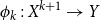 $\phi _k: X^{k+1} \to Y$
given by:
 \begin{align} \phi _0(x_0) &= \phi _Y(i, x_0) \nonumber \\ \phi _1(x_0, x_1) &= \phi _Y(\phi _S(i, x_0), x_1) \\ \phi _2(x_0, x_1, x_2) &= \phi _Y(\phi _S(\phi _S(i, x_0), x_1), x_2) \nonumber \\ \vdots \nonumber & \end{align}
When the gradient of
 $\Phi$
is needed at an input of length
 $k$
by a trainer, the gradient of
 $\phi _k$
at that input is used instead.
Taking the derivative of unrolled function is a useful procedure and is a basis of the machine learning algorithm called backpropagation through time (BPTT) (Werbos, Reference Werbos1990). However, its ad hoc nature raises some fundamental questions about the properties the procedure possesses. We study these formal properties and show that the differentiation of unrolled stateful functions enjoys a chain rule, a sum rule, a notion of partial derivative, and more. In particular, we are able to state the derivative of a stateful function as another stateful function, rather than a sequence of stateless functions. Roughly speaking, we accomplish this by taking advantage of the fact that the unrolling above is an iterated composition of
 $\phi$
with itself, and therefore its componentwise derivative can be “re-rolled” back into a single stateful function.
1.1 Outline
Our first main contribution is to give a construction which extends any given (Cartesian) category
 $\mathbb{C}$
, representing stateless functions, to a new category
 $\mathrm{St}(\mathbb{C})$
of stateful functions, particularly computations extended through discrete time (Definition 11). This
 $\mathrm{St}(\!-\!)$
construction captures causal functions as a special instance (Theorem13) and captures other stateful devices like Mealy machines and RNNs.
A distinctive feature of this construction includes the loop-with-delay gate seen in Figure 1, which we will more formally call a delayed trace operator (Definition 18). This delayed trace satisfies many of the properties of its better-known cousin, the trace operator of Joyal et al. (Reference Joyal, Street and Verity1996) (Proposition 19), but is missing the yanking condition and satisfies a modified form of dinaturality (Theorem20).
Our second major contribution is to give an abstract form of differentiation in this category of stateful computations. A key result of this paper is that if
 $\mathbb{C}$
is a Cartesian differential category (Blute et al., Reference Blute, Cockett and Seely2009), then so is
 $\mathrm{St}(\mathbb{C})$
(Theorem36). In particular, this differential operator matches the results obtained by unrolling-then-differentiating (Theorem37). The definition of Cartesian differential categories packages many of the classic properties of derivatives in a convenient abstract unit. Hence, showing that
 $\mathrm{St}(\mathbb{C})$
is a Cartesian differential category implicitly obtains a slew of fundamental results for differentiation of stateful computations.
1.2 Differences from the conference version
Much of the material in this work previously appeared in a conference paper (Sprunger and Katsumata, Reference Sprunger and Katsumata2019); here, we describe the differences. Section 2.3 revises Section II.C of the conference version (Sprunger and Katsumata, Reference Sprunger and Katsumata2019) about the relationship between causal functions and morphisms in
 $\mathrm{St}(\mathbb{C})$
. In this section, we define causal functions as families of functions depending on past inputs. We then show a new characterization of the category
 $\mathrm{St}(\mathbb{C})$
as the co-Kleisli category of a (generalized version of) Uustalu and Vene’s non-empty list comonad on
 $\mathbb{C}^{\mathbb{N}}$
. We remark that a similar result is shown for the category of monoidal streams (Lavore, de Felice, and Román, 2022, Theorem 6.3).
Section 5 has also been newly added. This section gives a functorial account of BPTT using the
 $\mathrm{St}(\!-\!)$
construction on a reverse Cartesian differential category. After the conference version (Sprunger and Katsumata, Reference Sprunger and Katsumata2019), Cockett et al. introduced these RCDCs (Cockett et al., Reference Cockett, Cruttwell, Gallagher, Pacaud Lemay, MacAdam, Plotkin, Pronk, Fernández and Muscholl2020), and Cruttwell et al. reformulated backpropagation for feedforward networks using the category of lenses (Cruttwell et al., Reference Cruttwell and Sergey2022); in their work, the reverse differential operator is treated as a functor
 $R:\mathbb{C}\to \mathrm{Lens}(\mathbb{C})$
to the category of lenses. We refine this functor by restricting
 $\mathrm{Lens}(\mathbb{C})$
to the category
 ${\mathrm{LLens}}(\mathbb{C})$
of linear lenses. We show that the restriction
 $\textbf{R}_l:\mathbb{C}\to{\mathrm{LLens}}(\mathbb{C})$
now preserves finite products, and the functor
 $\mathrm{St}(\textbf{R}_l):\mathrm{St}(\mathbb{C})\to \mathrm{St}({\mathrm{LLens}}(\mathbb{C}))$
computes the BPTT procedure.
2. Related Work
2.1 Categorical models of causal computations
Signal flow graphs are a widely used model of causal computation, especially in synchronous digital circuits and signal processing (Crochiere and Oppenheim, Reference Crochiere and Oppenheim1975; Parhi and Chen, Reference Parhi and Chen2013). The formation of loop paths in signal flow graphs are often restricted so that each loop path must go through at least one (initialized) delay gate. The delayed trace operator in
 $\mathrm{St}(\mathbb{C})$
in this paper embodies this principle.
A line of coalgebraic study of signal flow graphs by Rutten (Reference Rutten2005, Reference Rutten2008), Milius (Reference Milius2010), Hansen et al. (Reference Hansen, Kupke and Rutten2017), Basold et al. (Reference Basold, Bonsangue, Hansen and Rutten2014), and many others achieve characterizations of computable streams by signal flow graphs. This coalgebraic perspective makes it possible to apply powerful coalgebraic techniques to analyze the behavior of signal flow graphs. Our categorical work, on the other hand, regards signal flow graphs as morphisms in a certain category and focuses on the categorical structures realizing these flow graphs.
An axiomatic system for representing digital circuits based on monoidal category theory has been proposed by Ghica and Jung (2016) and Ghica et al., (2017). Their system is an extension of a traced cartesian category with a few structural morphisms that implement wire join and delay gate. Their delay gates do not support arbitrary initialization, but they can also represent interesting well-defined digital circuits using general loops without delay gates. The precise relationship between their axiomatic system and our categorical construction is not clear yet, and it is an interesting topic to investigate.
A category whose morphisms are realized by Mealy machine-like transducers is constructed in the memoryful GoI by Hoshino et al. (Reference Hoshino, Muroya and Hasuo2014). Their transducers, represented as functions of type
 $S\times A\rightarrow T(S\times B)$
, extend deterministic Mealy machines with the ability to perform computational effects represented by the monad
 $T$
. The machine type considered in our work does not support these abstract computational effects. Another technical difference from our work is that the monoidal structure on their category of transducers is based on finite coproducts in order to realize the particle-style trace operator for the GoI interpretation, whereas our work uses finite products.
Connections between category theory and machine learning have recently attracted significant interest (Fong et al., 2017). A notable example is Elliott (Reference Elliott2018), where Elliot studies automatic differentiation (AD) from the perspective of functional programming and category theory, obtaining Cartesian functors representing many AD algorithms.
Recently, Kissinger and Uijlen reformulated the concept of causality in quantum physics in a class of compact closed categories (Kissinger and Uijlen, Reference Kissinger and Uijlen2017). Starting from a compact closed category with some extra structure, they refine it to a *-autonomous category so that morphisms there respect causal constraints.
2.2 State and feedback
Categorical constructions enhancing a basic category with some form of statefulness go back to Katis et al. (1997). Similar constructions appear in the signal flow graph literature and the growing graphical linear algebra literature (Bonchi et al., 2014, Reference Bonchi, Rajamani and Walker2015, 2019). This line of work has a tradition of naming such constructions
 $\mathrm{St}(\!-\!)$
. The construction given in the latter work by Bonchi et al. (Reference Bonchi, Holland and Piedeleu2019) is very close to our
 $\mathrm{St}(\!-\!)$
construction. When it is applied to a compact closed PROP, it adjoins a one-input one-output generator to the PROP. However, it differs in that the semantics for these devices is relational, where ours is functional, and does not support arbitary initialization of delay gates.
Zanasi studies the PROP
 ${\mathbb{IH}}_R$
of interacting Hopf algebras over a ring
 $R$
in his PhD thesis (Zanasi, Reference Zanasi2015). The expressive power of this PROP is demonstrated by encoding various graphical systems into
 ${\mathbb{IH}}_R$
(Bonchi et al., Reference Bonchi, Baldan and Gorla2014, Reference Bonchi, Rajamani and Walker2015). When
 $R$
is the polynomial ring
 $k[x]$
over a field
 $k$
, the PROP
 ${\mathbb{IH}}_{k[x]}$
admits delay gates, and the trace-with-delay operation (which he called z-feedback operator) is definable (Bonchi et al., Reference Bonchi, Baldan and Gorla2014, Definition 7) and occupies a role analogous to the delay gate in our work.
At the moment of writing this paper, there are two papers that extend our
 $\mathrm{St}(\!-\!)$
construction. Carette et al. (Reference Carette, de Visme and Perdrix2021) give an extension of the
 $\mathrm{St}(\!-\!)$
construction to discard categories, symmetric monoidal categories with a designated family of maps to the monoidal unit. As they are interested in quantum computing with memory, they also allow additional limited non-causal observational effects such as postselection. To accommodate these actions, they further generalize from equality in our truncation condition to a monotonicity condition by requiring a further property for the discard category (pseudo-purifiability) that forces it to be preorder-enriched. In particular, all Cartesian categories are pseudo-purifiable discard categories, and their construction specializes to ours in this case.
Lavore et al. (2022) extended our
 $\mathrm{St}(\!-\!)$
construction to a certain class of monoidal categories called productive monoidal categories. Their extension is based on their observation that stateful morphism sequences belong to the final solution of a recursively defined set. They then pursued this idea and obtained the limit characterization of the construction. Superficially, their approach is different from our approach of quotienting the stateful morphism sequences by extensional equivalences. However, when the underlying monoidal category is Cartesian, their construction coincides with the
 $\mathrm{St}(\!-\!)$
construction in this paper. They also reformulated our delayed trace operator as a feedback operator in the sense of Katis, Sabadini, and Walters, with a modification of inserting an endofunctor.
Guardedness conditions on computations with feedback are a common theme (Abel and Pientka, Reference Abel, Pientka, Morrisett and Uustalu2013; Møgelberg, Reference Møgelberg2014). Goncharov and Schröder developed the theory of guarded traced categories to formalize this phenomena in Goncharov and Schröder (Reference Goncharov, Schröder, Baier and Lago2018). The key idea is to restrict Joyal et al.’s trace operator (Joyal et al., 1996) to a class of guarded morphisms, which are an abstractly given class of morphisms satisfying the guardedness condition. It is interesting to see the relationship between guarded trace operator and the delayed trace operator, and the key in this comparison is the treatment of the initial state.
Several research studies employ two-dimensional categorical structures to model state transition sytems. In Gadducci and Montanari’s tile model (Gadducci and Montanari, 2000), each tile
 $f:A\xrightarrow [S']{S} B$
represents a state transition from
 $A$
to
 $B$
, and
 $S$
and
 $S'$
represents the trigger and the effect of this transition. Baez and Master consider a double category of open Petri nets and give two styles of functorial semantics (Baez and Master, Reference Baez and Master2020). In their double category, 2-cells are to relate two open Petri nets modulo renaming of open ports. In this paper, we use double category to represent two axis of information flow, namely the axis for time elapse and the axis for information processing.
2.3 Categorical models of differentiation
Inspired by the semantics of differential
 $\lambda$
-calculus and differential proof nets by Ehrhard and Regnier (2003, 2005), Blute, Cockett, and Seely categorically formalized the differentiation operator in analysis. The formalization was first given in the categories where morphisms denote linear maps (Blute et al., Reference Blute, Cockett and Seely2006). Later, they introduced a new axiomatization (Blute et al., Reference Blute, Cockett and Seely2009) based on cartesian monoidal category where morphisms denote possibly nonlinear maps. This paper is based on the latter work and adopts more recent reformulations of differentiation operators studied in Cockett and Cruttwell (Reference Cockett and Cruttwell2014) and Cruttwell (Reference Cruttwell2017).
3. Preliminaries
We assume familiarity with basic category theory. If
 $\mathbb{C}$
is a category, we write
 $|\mathbb{C}|$
to denote its objects, and
 $\mathbb{C}(X, Y)$
to denote the homset for
 $X, Y \in |\mathbb{C}|$
. We may abbreviate an identity map
 ${\textrm{id}}_X$
to the name of its object,
 $X$
.
If
 $\mathbb{C}$
is a cartesian category, we write
 $1$
for its terminal object,
 $!_X:X\rightarrow 1$
for the unique maps to
 $1$
, and
 $\times$
for the product bifunctor. The tupling of morphisms
 $f_i:Y\rightarrow X_i$
for
 $i\in \{0,1\}$
is denoted by
 $\langle f_0,f_1 \rangle$
. Projections are denoted by
 $\pi ^{X_0,X_1}_i:X_0\times X_1\rightarrow X_i$
(
 $i\in \{0,1\}$
), and we drop the superscript when it is obvious from context. The symmetry map is denoted by
 $\sigma _{X, Y}: X\times Y \to Y\times X$
.
Bold metavariables—
 $\textbf{X},\textbf{s}$
, etc.—denote infinite sequences of mathematical objects, indexed by
 $\mathbb{N}$
. The
 $i$
th component of a sequence is
 $\textbf{X}_i$
. By
 $\mathop{\bigcirc }{\textbf{X}}$
, we mean the tail of
 $\textbf{X}$
, namely
 $\mathop{\bigcirc }\textbf{X}=\textbf{X}_1,\textbf{X}_2,\cdots$
. In addition to Roman letter subscripts, we use a dot
 $\bullet$
as a special index variable, which can be bound by the sequence-forming bracket notation given next.
Let
 $e$
be an expression containing some dotted sequence metavariables
 $\textbf{X}_\bullet, \textbf{Y}_\bullet \cdots$
. By
 $[e]$
, we mean the infinite sequence obtained by substituting
 $0,1,2\cdots$
for
 $\bullet$
. For instance,
 $(i,[\textbf{x}_\bullet +\textbf{y}_\bullet ]) \,\text{is}\, (i, \textbf{x}_0+\textbf{y}_0,\,\textbf{x}_1+\textbf{y}_1,\,\cdots )$
and
 $[(i,\textbf{x}_\bullet +\textbf{y}_\bullet )] \,\text{is}\, (i,\textbf{x}_0+\textbf{y}_0),\,(i,\textbf{x}_1+\textbf{y}_1),\,\cdots$
.
When
 $e$
contains at least one dotted sequence metavariable, we may omit the outermost
 $[-]$
, so
 $[\textbf{X}_\bullet \times \textbf{Y}_\bullet ]$
may be written as
 $\textbf{X}_\bullet \times \textbf{Y}_\bullet$
. This omission is not allowed when
 $e$
contains no such variable; otherwise, we would confuse ordinary expressions (like
 $x+y$
) and constant infinite sequences (like
 $[x+y]=x+y,x+y,\cdots$
).
A mathematical formula
 $\phi$
containing dotted sequence metavariables represents the conjunction
 $\bigwedge _{i\in{\mathbb{N}}}\phi [i/\!\bullet\!]$
. For instance,
 ${\textbf{Z}}_\bullet ={\textbf{X}}_\bullet \times{\textbf{Y}}_\bullet$
means
 $\forall i\in{\mathbb{N}} \cdot \textbf{Z}_i=\textbf{X}_i\times \textbf{Y}_i$
.
4. Extending Cartesian Categories along Discrete Time
Before jumping into the depths of categorical abstraction, we consider different kinds of functions on sequences and particularly where causal functions lie.
One natural way to obtain functions on sequences is to consider the category
 $\textbf{Set}^{\mathbb{N}}$
, the countable product category of
 $\textbf{Set}$
. In this category, each morphism
 $\textbf{f}:\textbf{X}\rightarrow \textbf{Y}$
consists of independent components
 $\textbf{f}_k:\textbf{X}_k\rightarrow \textbf{Y}_k$
for all
 $k \in{\mathbb{N}}$
, each computing a single entry in the output sequence.
These are functions taking sequences to sequences in a causal manner, but the
 $k$
th output of
 $\textbf{f}$
depends only on the
 $k$
th input, not on all inputs before
 $k$
. Therefore, some causal functions of sequences, such as computing a running average, are missing from this class.
Another natural idea would be to take all the functions in homsets
 $\textbf{Set}(\prod \textbf{X}, \prod \textbf{Y})$
for arbitrary
 $\textbf{X}, \textbf{Y} \in |\textbf{Set}^{\mathbb{N}}|$
. This class is too big—non-causal functions such as
 ${\tt tl}: (x_0, x_1, \ldots ) \mapsto (x_1, x_2, \ldots )$
are present there. Therefore, we must do something a bit more complex to obtain the class of causal functions somewhere between these two.
To obtain causal functions, we return to our original idea,
 $\textbf{Set}^{\mathbb{N}}$
, and add objects in the domain and codomain of each component of
 $\textbf{f}$
representing communication channels with its neighboring components, like
 \begin{equation} \textbf{f}_k:\textbf{S}_k\times \textbf{X}_k\rightarrow \textbf{S}_{k+1}\times \textbf{Y}_k. \end{equation}
To start this computation, we also need to provide an initial state
 $i:1\rightarrow \textbf{S}_0$
. We call the pair
 $(i,\textbf{f})$
a stateful morphism sequence. We will see causal functions are equivalence classes of these stateful morphism sequences (Theorem13).
Though these are functions on sequences, it will often be convenient to pretend that these sequences are produced one element at a time, synchronized by some clock signal. Thus, since the function
 $\textbf{f}_k$
above computes the
 $k$
th element in the sequence, we may refer to it as producing a value at clock tick
 $k$
. Similarly, we refer to the element of state passed from
 $\textbf{f}_k$
to
 $\textbf{f}_{k+1}$
as being kept across clock ticks, and other such language. In this way, computing functions of sequences can also be thought of as performing discrete timed computations.
There is a clear distinction between the roles of
 $\textbf{X}_k/\textbf{Y}_k$
and
 $\textbf{S}_k/\textbf{S}_{k+1}$
—the former objects are the types of values flowing through
 $\textbf{f}_k$
at clock tick
 $k$
, while the latter objects are the types of states passed across clock ticks. We organize these two different kinds of information flow using special two-dimensional categories called double categories (Ehresmann, 1963).
Roughly speaking, double categories consist of 0-cells (objects), two types of 1-cells (horizontal and vertical morphisms), and 2-cells (tiles) which go between pairs of horizontal and vertical 1-cells. These 2-cells are often drawn as in Figure 3a.
2-cells in a double category.

These tiles can be composed along either common vertical 1-cells (horizontal composition) or common horizontal 1-cells (vertical composition). Having these two distinct types of composition available is the essential and only reason for using a double category in this paper so that we can use one composition for composition within a clock tick and the other for composition across clock ticks. We will not be using any results of higher category theory or further higher-dimensional abstractions.
Our double category will therefore have a particularly simple structure, with 2-cells as depicted in Figure 3b. We have a dummy 0-cell (
 $\cdot$
), objects from
 $\mathbb{C}$
as 1-cells, representing values when oriented vertically and states when oriented horizontally, and functions
 $\textbf{f}_k$
on states and values in the tiles.
Definition 1.
Let
 $(\mathbb{C}, \times, 1)$
be a strict Cartesian category. The double category
 $Dbl(\mathbb{C})$
is defined as follows:
-
• The set of objects (0-cells) is
 $\{\cdot \}$
.
-
• Horizontal and vertical 1-cells are both given by objects of
$\mathbb{C}$
, composed with
$\times$
, and have
$1$
as the identity.
-
• A 2-cell
$f$
with source horizontal 1-cell
$S$
, source vertical 1-cell
$X$
, target horizontal 1-cell
$S'$
, and target vertical 1-cell
$Y$
is a morphism
$\phi \in \mathbb{C}(S\times X, S'\times Y)$
.As indicated in Figure 3c, we denote the source and target 1-cells of
$f$
(
$S, X, S',$
and
$Y$
) by
$\mathop{\mathrm{prv}} f, \mathop{\mathrm{dom}} f, \mathop{\mathrm{nxt}} f,$
and
$\mathop{\mathrm{cod}} f$
, respectively. We will generally denote a 2-cell by
$f:X\xrightarrow [S']{S} Y$
. We call
$\phi$
the underlying morphism of
$f$
, while
$U$
is the operation taking a 2-cell to its underlying morphism, so
$U\;f = \phi$
. -
• The horizontal composition of 2-cells, say the
$f$
above before
$g:Y\xrightarrow [T']{T} Z$
, is
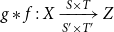
$g* f: X\xrightarrow [S'\times T']{S\times T}Z$
with underlying morphism
$U\,(g * f) \mathbin{\triangleq } (S' \times U\;g)\circ (\sigma _{S', T}\times Y)\circ (T \times U\;f)\circ (\sigma _{S, T}\times X)$
. -
• The vertical composition of 2-cells, say the
$f$
above before
$h:V\xrightarrow [S'']{S'} W$
, is
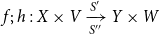
$f ;\; h:X \times V\xrightarrow [S'']{S'}{Y\times W}$
with underlying morphism
$U\,(f;\; h) \mathbin{\triangleq } (S'' \times \sigma _{Y, W})\circ (U\;h\times Y)\circ (S'\times \sigma _{V,Y})\circ (U\;f\times V)$
.












NB: vertical composition is given in relational composition order, while horizontal composition is given in functional composition order.
The strictness of
 $\times$
is important in this definition so that 1-cell composition is associative. It is possible that a better definition for
 $Dbl(\mathbb{C})$
might obviate this technical restriction, but for now we sacrifice a bit of generality to avoid working with associators and unitors. When we want to use this construction on a non-strict Cartesian category
 $\mathbb{C}$
, we instead follow Mac Lane (Lane, Reference Mac Lane1998, p. 257) and supply an equivalent Cartesian category
 $\mathbb{C}^s$
defined by:
-
• objects are finite lists of
$\mathbb{C}$
-objects, and -
•
$\mathbb{C}^s((A_1,\cdots, A_n),(B_1,\cdots, B_m))= \mathbb{C}\left (\prod A_i,\prod B_j\right )$
.


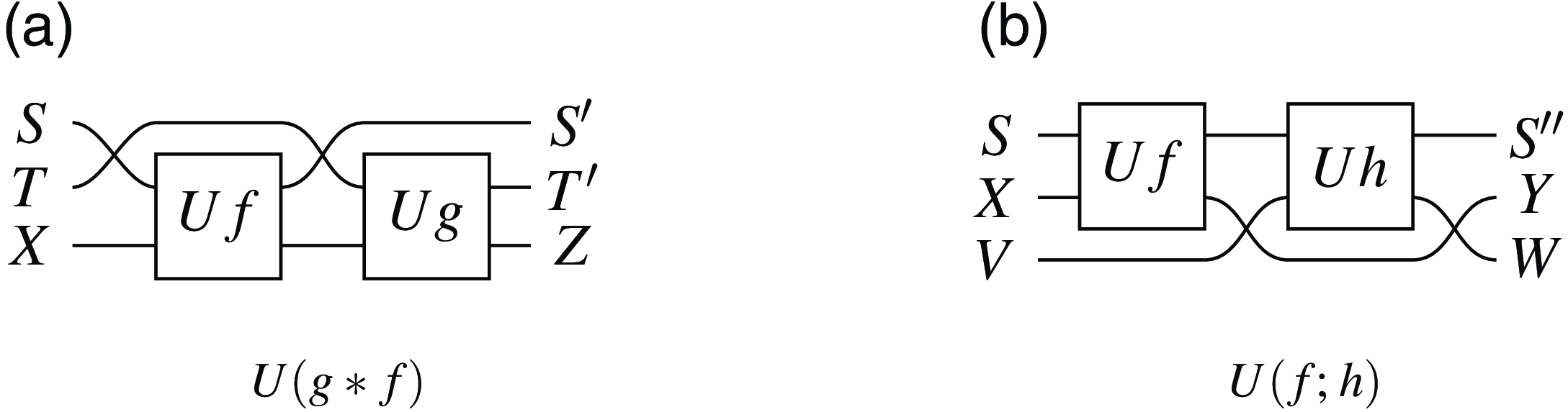
String diagrams for the underlying
 $\mathbb{C}$
-morphisms of horizontal and vertical composites may be helpful to digest this definition. The underlying morphisms of the horizontal composition
 $g* f$
and vertical composition
 $f;\; h$
are shown in Figure 4.
Underlying morphisms for composites of 2-cells.

A 2-cell
 $f$
of
 $Dbl(\mathbb{C})$
is determined by its underlying morphism
 $\phi$
from
 $\mathbb{C}$
. To stress this, we often draw
 $\phi$
inside the tile, with its inputs and outputs connected to corresponding edges:

Horizontal composition of 2-cells is composition along values like
 ${\textbf{X}}_\bullet$
or
 ${\textbf{Y}}_\bullet$
, and we think of as occurring within a single clock tick. Vertical composition is composition along states like
 ${\textbf{S}}_\bullet$
and occurs across clock ticks.
Definition 2.
For
 $\phi \in \mathbb{C}(X,Y)$
, the 2-cells
 $\phi ^h:X\xrightarrow [1]{1} Y$
and
 $\phi ^v: 1\xrightarrow [Y]{X}1$
have
 $U(\phi ^h) \mathbin{\triangleq } \phi \mathbin{\triangleq } U(\phi ^v)$
.
These operations sending
 $\mathbb{C}$
-morphisms to 2-cells in
 $Dbl(\mathbb{C})$
are particularly useful. (Note first that
 ${\textrm{id}}_X^h$
are identities for horizontal composition, and similarly
 ${\textrm{id}}_S^v$
are identities for vertical composition!) More practically, 2-cells of the form
 $\phi ^h$
modify values only, while 2-cells of the form
 $\phi ^v$
modify states only.
Lemma 3.
If
 $f:X\xrightarrow [S']{S} Y$
is a
 $Dbl(\mathbb{C})$
2-cell,
 $\phi _1 \in \mathbb{C}(T, S)$
,
 $\phi _2 \in \mathbb{C}(S', T')$
,
 $\psi _1 \in \mathbb{C}(W, X)$
, and
 $\psi _2 \in \mathbb{C}(Y, Z)$
, then the underlying morphism of
 $\phi _1^v;\;(\psi _2^h* f * \psi _1^h);\; \phi _2^v$
has the following string diagram in
 $\mathbb{C}$
:

Note that if
 $\phi _2$
and
 $\psi _2$
are identities, the composed 2-cell above is denoted
 $\phi _1^v;\; f* \psi _1^h$
. This compact notation for precomposition in both dimensions is a powerful notational advantage of having the
 $;$
and
 $*$
operators take their arguments in different orders.
4.1 Stateful morphism sequences and extensional equivalence
Each 2-cell of the double category
 $Dbl(\mathbb{C})$
represents an individual component computing a single output value in a time-extended computation, like that of Eq. (2). To represent a whole causal computation, we collect together countably many of these components into a stateful morphism sequence.
Definition 4.
Let
 $\textbf{X},\textbf{Y}\in |\mathbb{C}|^{\mathbb{N}}$
be sequences of
 $\mathbb{C}$
-objects. A stateful morphism sequence of type
 $\textbf{X}\rightarrow \textbf{Y}$
is a pair
 $(i,\textbf{s})$
of a sequence
 $\textbf{s}$
of 2-cells in
 $Dbl(\mathbb{C})$
and a
 $\mathbb{C}$
-morphism
 $i :1\rightarrow \mathop{\mathrm{prv}}\textbf{s}_0$
such that
 $\mathop{\mathrm{dom}}{\textbf{s}_\bullet }=\textbf{X}_\bullet$
,
 $\mathop{\mathrm{cod}}{\textbf{s}_\bullet }=\textbf{Y}_\bullet$
, and
 $\mathop{\mathrm{nxt}}{\textbf{s}_\bullet }=\mathop{\mathrm{prv}}{\textbf{s}_{\bullet +1}}$
. The state sequence of
 $(i,\textbf{s})$
is
 $\mathrm{st}(i,\textbf{s}) \mathbin{\triangleq } [\mathop{\mathrm{prv}}(\textbf{s}_\bullet )]$
.
Note the last condition implies
 $\textbf{s}_\bullet ;\; \textbf{s}_{\bullet +1}$
exists, which allows each component to pass state to the next.
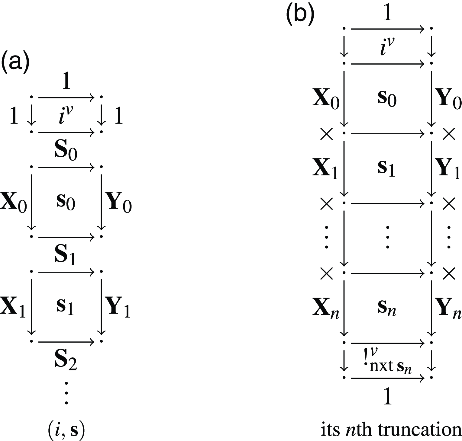
A stateful morphism sequence can be thought of as an infinite tower of 2-cells, each layer of which is vertically composable with adjacent layers, as depicted in Figure 5a.
A stateful morphism sequence and a truncation.

In this representation, the “arrow of time” starts at
 $\textbf{X}_0$
and points down. At the zeroth clock tick, the stateful morphism sequence receives a value at
 $\textbf{X}_0$
, outputs a value at
 $\textbf{Y}_0$
, and sets a state value of type
 $\textbf{S}_1$
. Then at the first clock tick, the first layer of the stateful morphism sequence executes, using the state previously prepared by the zeroth layer.
Since we intend the state maintained by these sequences to be internal, saying
 $(i,\textbf{s}) = (j,\textbf{t})$
if and only if they are exactly the same sequence of 2-cells is not a suitable notion of equality. Ideally, if we could form the infinite vertical composition of 2-cells, the natural definition of equality of two stateful morphism sequences of type
 $\textbf{X}\rightarrow \textbf{Y}$
would be to compare the underlying
 $\mathbb{C}$
-morphisms of the infinite composition, meaning
 $(i, \textbf{s}) = (j, \textbf{t})$
if and only if
 \begin{align*} U(i^v;\;\textbf{s}_0;\;\textbf{s}_1;\;\cdots )=U(j^v;\;\textbf{t}_0;\;\textbf{t}_1;\;\cdots ): \prod _{k\in{\mathbb{N}}}\textbf{X}_k\rightarrow \prod _{k\in{\mathbb{N}}}\textbf{Y}_k. \end{align*}
However, formalizing this infinite vertical composition is technically challenging, and
 $\mathbb{C}$
may not have countable products. We therefore instead require that all finite initial segments of the sequence match using a truncation operation.
Definition 5.
The
 $n$
th truncation of a stateful morphism sequence
 $(i,\textbf{s}):\textbf{X}\rightarrow \textbf{Y}$
is the
 $\mathbb{C}$
-morphism
 \begin{align*} \mathrm{Tc}_n(i,\textbf{s}) &\mathbin{\triangleq } U(i^v ;\; \textbf{s}_0 ;\; \cdots ;\; \textbf{s}_n;\; !_{\mathop{\mathrm{nxt}} \textbf{s}_n}^v) : \prod _{k=0}^n\textbf{X}_k\rightarrow \prod _{k=0}^n\textbf{Y}_k. \end{align*}
Graphically,
 $\mathrm{Tc}_n(i,\textbf{s})$
is the underlying morphism of the vertical composite 2-cell depicted in Figure 5a.Footnote
2
Definition 6.
Two stateful morphism sequences
 $(i,\textbf{s}),(j,\textbf{t}):\textbf{X}\rightarrow \textbf{Y}$
are extensionally equal iff
 $\mathrm{Tc}_\bullet (i, \textbf{s}) = \mathrm{Tc}_\bullet (j, \textbf{t})$
.
It is easy to verify that extensional equality between stateful morphism sequences is an equivalence relation.
The state sequences of extensionally equivalent stateful morphisms sequences can be different, which is good because it matches our intention and bad because it can be harder to decide whether two computation sequences are equal. Comparing truncations is always possible, but sometimes technically difficult. The following lemma has proven a useful method for establishing extensional equality.
Lemma 7 (Shim lemma).Footnote
3
Suppose
 $(i, \textbf{s}),(j, \textbf{t}):\textbf{X}\rightarrow \textbf{Y}$
are stateful morphism sequences, and
 $\textbf{b}$
is a sequence of
 $\mathbb{C}$
-morphisms such that
 $\textbf{b}_\bullet :\mathop{\mathrm{prv}}(\textbf{s}_\bullet )\rightarrow \mathop{\mathrm{prv}}(\textbf{t}_\bullet )$
,
 $\textbf{b}_0\circ i = j$
, and
 $\textbf{s}_\bullet ;\; \textbf{b}_{\bullet +1}^v = \textbf{b}_\bullet ^v ;\; \textbf{t}_\bullet$
. Then
 $(i, \textbf{s})$
and
 $(j, \textbf{t})$
are extensionally equivalent.
Proof. Show by induction that
 \begin{equation*}i^v;\;\textbf {s}_0;\;\cdots ;\;\textbf {s}_n;\; \textbf {b}_{n+1}^v;\; !_{\mathop {\mathrm {nxt}}{\textbf {t}_n}}^v = j^v;\;\textbf {t}_0;\;\cdots ;\; \textbf {t}_n;\; !_{\mathop {\mathrm {nxt}}{\textbf {t}_n}}^v\end{equation*}
Unrolling and truncation are related operations, and in fact we can extend unrolling to general stateful morphism sequences.
Definition 8.
Let
 $(i,\textbf{s}):\textbf{X}\rightarrow \textbf{Y}$
be a stateful morphism sequence. Its
 $n$
-th unrolling is the
 $n$
th projection of the
 $n$
th truncation:
 $\mathrm{Un}_n(i,\textbf{s})\mathbin{\triangleq } \pi _n\circ \mathrm{Tc}_n(i,\textbf{s}):\prod _{k=0}^n\textbf{X}_k\rightarrow \textbf{Y}_n$
.
For instance, the recurrently defined functions
 $\phi _n$
in section 1 are unrollings of a certain stateful morphism sequence involving
 $\phi$
and
 $i$
.
4.2 Category of Causal morphisms
We are ready to construct our category of causal morphisms using stateful morphism sequences and extensional equality between them.
Definition 9.
The identity stateful morphism sequence
 ${\textrm{id}}_{\textbf{X}}$
is
 $({\textrm{id}}_1,[({\textrm{id}}_{\textbf{X}_\bullet })^h])$
for all
 $\textbf{X} \in |\mathbb{C}|^{\mathbb{N}}$
.
The composition of two stateful morphism sequences
 $(i,\textbf{s}):\textbf{Y}\rightarrow \textbf{Z}$
and
 $(j,\textbf{t}):\textbf{X}\rightarrow \textbf{Y}$
is
 \begin{align*} (i,\textbf{s})\circ (j,\textbf{t})\mathbin{\triangleq } (\langle j, i\rangle, [{\textbf{s}}_\bullet *{\textbf{t}}_\bullet ]):\textbf{X}\rightarrow \textbf{Z}. \end{align*}
As usual, we may denote
 ${\textrm{id}}_{\textbf{X}}$
by
 $\textbf{X}$
.
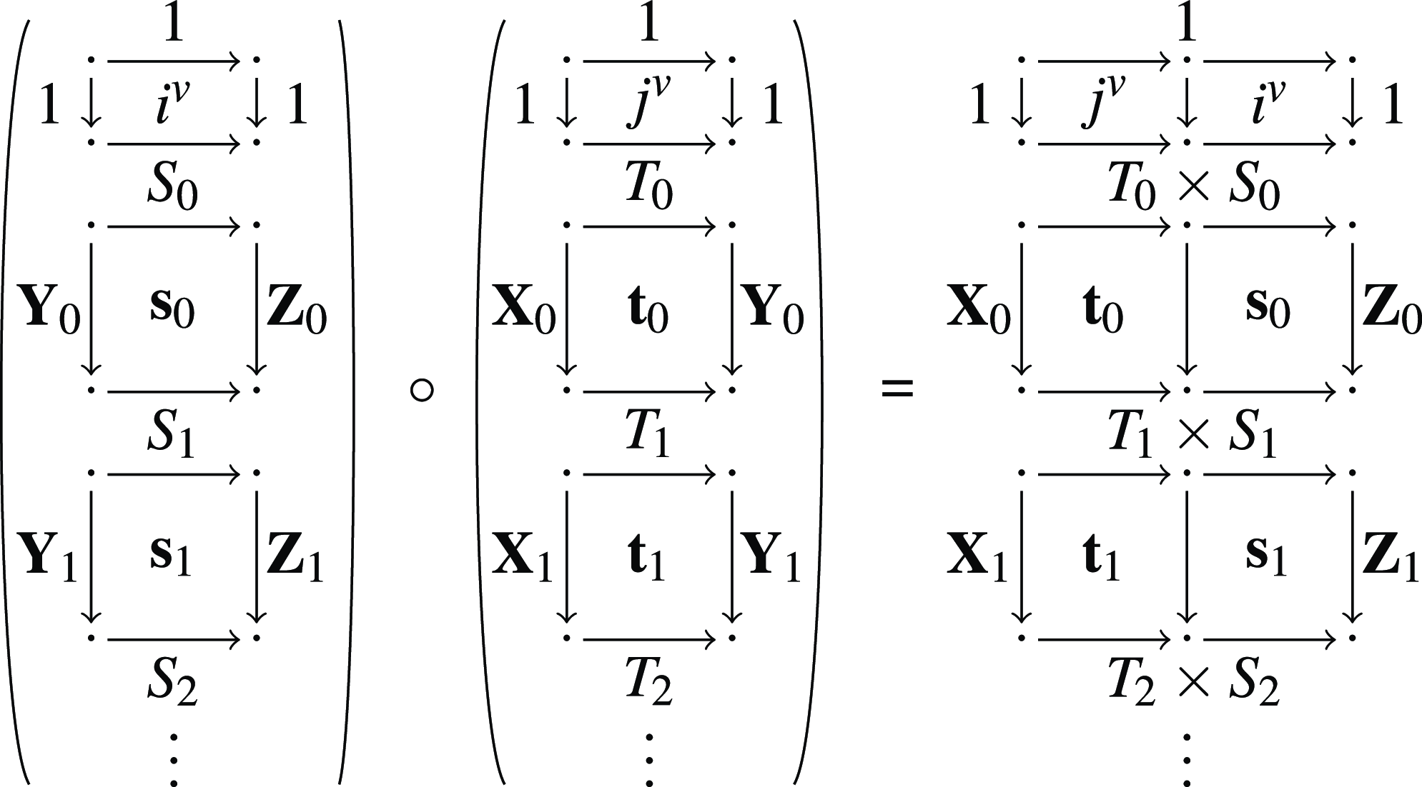
Composition of stateful morphism sequences.

In our “tower of 2-cells” representation, the composition of stateful morphism sequences is in Figure 6. Note the state sequence of the composite is the componentwise product of the original state sequences.
Lemma 10.
Composition of stateful morphism sequences is well defined on extensional equivalence classes. Further, (the extensional equivalence class of)
 ${\textrm{id}}_{\textbf{X}}$
is the unit for the composition operation.
Definition 11.
Given a Cartesian category
 $\mathbb{C}$
, its causal extension is a category
 $\mathrm{St}(\mathbb{C})$
where
-
• objects are
$|\mathbb{C}|^{\mathbb{N}}$
, that is,
$\mathbb{N}$
-indexed families of
$\mathbb{C}$
-objects,
-
• morphisms are extensional equivalence classes of stateful morphism sequences,
-
• identities and composition are the extensions of those in Definition 9 to the extensional equivalence classes by Lemma 10 .


We will justify our use of the word “causal” by establishing a connection to another formalization of causal functions in Theorem13, but first we establish some properties of
 $\mathrm{St}(\mathbb{C})$
.
The category
 $\mathbb{C}^{\mathbb{N}}$
is naturally included into
 $\mathrm{St}(\mathbb{C})$
via the functor
 $H:\mathbb{C}^{\mathbb{N}}\rightarrow \mathrm{St}(\mathbb{C})$
:
 \begin{align*} H\textbf{X}&=\textbf{X}, & H\textbf{f}&=({\textrm{id}}_1,[\textbf{f}_\bullet ^h]). \end{align*}
We call the morphisms in
 $\mathrm{St}(\mathbb{C})$
of the form
 $H\textbf{f}$
stateless morphisms, since they can be realized by a stateful morphism sequence whose state sequence is constantly 1, that is,
 $[1]$
.
Proposition 12.
 $\mathrm{St}(\mathbb{C})$
is Cartesian, and
 $H$
is finite-product preserving.
Proof. In
 $\mathrm{St}(\mathbb{C})$
, the final object is
 $[1]$
and the final map from
 $\textbf{X}$
is
 $H[{!_{{\textbf{X}}_\bullet }}]$
. Products and projection are also componentwise: our chosen
 $\mathrm{St}(\mathbb{C})$
product
 $\textbf{X}\times \textbf{Y}$
is the sequence
 $[{\textbf{X}}_\bullet \times{\textbf{Y}}_\bullet ]$
of
 $\mathbb{C}$
products, with
 $\pi _n \mathbin{\triangleq } H[\pi _n^{{\textbf{X}}_\bullet, {\textbf{Y}}_\bullet }]$
for
 $n \in \{0, 1\}$
.
We extend the truncation
 $\mathrm{Tc}$
operation and the unrolling operation
 $\mathrm{Un}$
to morphisms in
 $\mathrm{St}(\mathbb{C})$
. They are now regarded as the following functions on homsets:
 \begin{align*} \mathrm{Tc}_n&:\mathrm{St}(\mathbb{C})(\textbf{X},\textbf{Y})\to \mathbb{C}\left (\prod _{k=0}^n\textbf{X}_k,\prod _{k=0}^n\textbf{Y}_k\right ), & \mathrm{Un}_n&:\mathrm{St}(\mathbb{C})(\textbf{X},\textbf{Y})\to \mathbb{C}\left (\prod _{k=0}^n\textbf{X}_k,\textbf{Y}_n\right ). \end{align*}
We also extend the
 $\mathrm{St}(\!-\!)$
construction to functors. Let
 $\mathbb{C},\mathbb{D}$
be strict Cartesian categories and
 $F:\mathbb{C}\to \mathbb{D}$
be a functor that strictly preserves finite products. We define
 $\mathrm{St}(F):\mathrm{St}(\mathbb{C})\to \mathrm{St}(\mathbb{D})$
by:
 \begin{align*} \mathrm{St}(F)(\textbf{X})&=[F(\textbf{X}_\bullet )] & \mathrm{St}(F)(i,\textbf{s})&=(Fi,[F(\textbf{s}_\bullet )]). \end{align*}
When
 $F$
only preserves finite products, insert appropriate canonical isomorphisms around
 $F\textbf{s}_\bullet$
.
4.3 Morphisms in
$\mathrm{St}(\mathbb{C})$
and Causal morphisms

We claim that morphisms of
 $\mathrm{St}(\mathbb{C})$
represent causal computations, whose outputs depend only on past inputs and states. To justify this claim, we compare causal computations as functions depending on past inputs and morphisms in
 $\mathrm{St}(\mathbb{C})$
for a strict Cartesian category
 $\mathbb{C}$
.
What is a causal computation from
 $\textbf{X}$
to
 $\textbf{Y}$
? Suppose
 $f$
is such a computation. Then the output at time
 $n$
is computed from all the inputs up to time
 $n$
. Therefore the input-output relationship at time
 $n$
is given by a function
 $f_n:\textbf{X}_0\times \cdots \times \textbf{X}_n\to \textbf{Y}_n$
, and the collection of all such functions represents a causal computation from
 $\textbf{X}$
to
 $\textbf{Y}$
. We thus regard the family
 $f\triangleq \{f_n\}_{n\in{\mathbb{N}}}$
as the entity embodying a causal computation and naturally view it as a morphism in
 $\mathbb{C}^{\mathbb{N}}$
(the
 $\mathbb{N}$
-fold product category of
 $\mathbb{C}$
).
We point out that
 $f$
is a morphism in the co-Kleisli category of a comonad
 $D$
on
 $\mathbb{C}^{\mathbb{N}}$
. This comonad’s functor part is given by
 $ D(\textbf{X})_n\triangleq \textbf{X}_0\times \cdots \times \textbf{X}_n.$
This is a refinement of Uustalu and Vene’s non-empty list comonad capturing causal stream functions (Uustalu and Vene, Reference Uustalu and Vene2005). The difference is that
 $D$
is defined over the category
 $\mathbb{C}^{\mathbb{N}}$
of time-varying objects and morphisms, while their comonad is defined over a Cartesian category with countable coproducts. Indeed, Uustalu and Vene’s non-empty list comonad is
 $\Sigma \circ D\circ \Delta$
, where
 $\Sigma \dashv \Delta :\mathbb{C}\to \mathbb{C}^{\mathbb{N}}$
is the adjunction arising from the countable coproduct in
 $\mathbb{C}$
.
We show that the causal computations modeled by co-Kleisli morphisms of
 $D$
coincides with those modeled by
 $\mathrm{St}(\mathbb{C})$
-morphisms. This isomorphism morally states the coincidence of memoryful computations and causal computations.
Theorem 13.
 $(\mathbb{C}^{\mathbb{N}})_D\cong \mathrm{St}(\mathbb{C})$
.
In Lavore, de Felice, and Román (2022) (Theorem 6.3), the co-Kleisli category
 $(\mathbb{C}^{\mathbb{N}})_D$
is shown to be isomorphic to the category of monoidal streams over
 $\mathbb{C}$
, which is differently constructed from the
 $\mathrm{St}(\!-\!)$
construction.
Proof. We first decompose
 $D$
into an adjunction. Let
 $\iota :{\mathbb{N}}\to \omega ^{op}$
be the inclusion of the discrete poset
 $\mathbb{N}$
into the opposite of the poset
 $\omega$
of finite ordinals. The precomposition functor
 ${-}\circ \iota :\mathbb{C}^{\omega ^{op}}\to \mathbb{C}^{\mathbb{N}}$
has a right adjoint given by the right Kan extension
 $R$
along
 $\iota$
:

It sends an object
 $\textbf{X}\in \mathbb{C}^{\mathbb{N}}$
to the sequence of prefix projections:

In particular, its object part is given by
 $(R\textbf{X})_n=\prod _{i=0}^n\textbf{X}_i$
. We note that the projection
 $c_{\textbf{X},n}:{\textbf{X}}_0\times \cdots \times{\textbf{X}}_{n+1} \rightarrow{\textbf{X}}_0\times \cdots \times{\textbf{X}}_{n}$
can be given as
 $c_{\textbf{X},n} \triangleq U ({\textrm{id}}_{{\textbf{X}}_0}^h ; \ldots ;{\textrm{id}}_{{\textbf{X}}_n}^h ; !_{{\textbf{X}}_{n + 1}}^h)$
.
For brevity, let
 $L={-}\circ \iota$
. It holds
 $L\circ R(\textbf{X})=D(\textbf{X})$
, and
 $D$
acquires a comonad structure from the adjunction
 $L\dashv R$
. Therefore to show the theorem, it suffices to exhibit an isomorphism on homsets:
 $ \Phi _{\textbf{X},\textbf{Y}}:\mathrm{St}(\mathbb{C})(\textbf{X},\textbf{Y})\cong \mathbb{C}^{\omega ^{op}}(R \textbf{X},R \textbf{Y})$
. Define
 \begin{align*} (\Phi _{\textbf{X},\textbf{Y}}(i,\textbf{s}))_n\triangleq \mathrm{Tc}_n(i,\textbf{s}). \end{align*}
This is a good definition, as
 $(i,\textbf{s})$
is an extensional equivalence class.
We first show that
 $\Phi$
(or equivalently
 $\mathrm{Tc}$
) is natural in
 $n$
. By unfolding the definition, we obtain
 \begin{eqnarray*} c_{\textbf{Y}, n} \circ \mathrm{Tc}_{n + 1} (i,{\textbf{s}}) = U (i^v ;\;{\textbf{s}}_0 ; \ldots ; (!_{{{\textbf{Y}}}_{n + 1}}^h \ast{\textbf{s}}_{n + 1}) ; !^v_{S_{n + 2}}) . \end{eqnarray*}
The vertical composition of the last two 2-cells satisfies
 $U ((!_{{{\textbf{Y}}}_{n + 1}}^h \ast s_{n + 1}) ; !^v_{S_{n + 2}}) ={!^v_{S_{n + 1}}} \ast{!_{{\textbf{X}}_{n + 1}}^h} .$
Therefore,
 \begin{eqnarray*} U (i^v ;\;{\textbf{s}}_0 ; \ldots ; (!_{{{\textbf{Y}}}_{n + 1}}^h \ast{\textbf{s}}_{n + 1}) ;\; !^v) & = & U (i^v;\;{\textbf{s}}_0 ; \ldots{\textbf{s}}_n ;\; ({!^v_{S_{n + 1}}} \ast{!_{{\textbf{X}}_{n + 1}}^h}))\\ & = & U (i^v ;\;{\textbf{s}}_0 ;\; \ldots ;{\textbf{s}}_n ;\; !_{S_{n + 1}}^v) \circ U ({\textrm{id}}_{{\textbf{X}}_0}^h ;\; \ldots ;\;{\textrm{id}}_{{\textbf{X}}_n}^h ;\; !_{{\textbf{X}}_{n + 1}}^h)\\ & = & \mathrm{Tc}_n (i,{\textbf{s}}) \circ c_{\textbf{X}, n}. \end{eqnarray*}
This ends the proof of naturality.
We next define
 ${l}_{{\textbf{X}}, \bullet } : (R{\textbf{X}})_\bullet \rightarrow{\textbf{X}}_{\bullet }$
to be the projection of the last component. Since we are working in a strict Cartesian category, we have
 ${l}_{{\textbf{X}}, 0} ={\textrm{id}}_{{\textbf{X}}_0}$
and
 $\langle{c}_{{\textbf{X}}, \bullet -1 },{l}_{{\textbf{X}}, \bullet } \rangle ={\textrm{id}}_{(R{\textbf{X}})_\bullet }$
.
We show the surjectivity of
 $\Phi$
. Let
 $\alpha : R{\textbf{X}} \rightarrow R{\textbf{Y}}:\omega ^{op}\to \mathbb{C}$
be a natural transformation. We define 2-cells
 $i_{\alpha }:1\xrightarrow [1]{1}1$
by
 $i_{\alpha } \triangleq{\textrm{id}}_1^v$
and
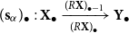 $({\textbf{s}}_\alpha )_\bullet : {\textbf{X}}_\bullet \xrightarrow [(R{\textbf{X}})_\bullet]{(R{\textbf{X}})_{\bullet -1}}{{\textbf{Y}}_\bullet }$
by (below
 $\delta$
is the diagonal morphism):
 \begin{align*} ({\textbf{s}}_\alpha )_\bullet \triangleq ({\textrm{id}}_{(R{\textbf{X}})_\bullet } \times ({l}_{{\textbf{Y}}, \bullet } \circ \alpha _\bullet )) \circ \delta _{(R{\textbf{X}})_\bullet } : (R{\textbf{X}})_{\bullet -1}\times{\textbf{X}}_\bullet =(R{\textbf{X}})_\bullet \rightarrow (R{\textbf{X}})_\bullet \times{\textbf{Y}}_\bullet . \end{align*}
We show the following equality by induction, which is sufficient to show
 $\Phi (i_\alpha, {\textbf{s}}_\alpha ) = \alpha$
:
 \begin{equation} U (i_{\alpha } ;\; ({\textbf{s}}_\alpha )_0 ; \ldots ; ({\textbf{s}}_\alpha )_\bullet ) = ({\textrm{id}}_{(R{\textbf{X}})_\bullet } \times \alpha _\bullet ) \circ \delta _{(R{\textbf{X}})_\bullet }. \end{equation}
The case
 $n = 0$
is trivial. We show the induction case. First, a diagrammatic calculation using the induction hypothesis shows
 \begin{align*} U (i_{\alpha } ;\; ({\textbf{s}}_\alpha )_0 ; \ldots ; ({\textbf{s}}_\alpha )_{n + 1}) = ({\textrm{id}}_{(R{\textbf{X}})_{n + 1}} \times \langle \alpha _n \circ{c}_{{\textbf{X}}, n + 1},{l}_{{\textbf{X}}, n + 1} \circ \alpha _{n + 1} \rangle ) \circ \delta _{(R{\textbf{X}})_{n + 1}} . \end{align*}
Then from the naturality of
 $\alpha$
, the tupled morphism part satisfies
 \begin{align*} \langle \alpha _n \circ{c}_{{\textbf{X}}, n + 1},{l}_{{\textbf{X}}, n + 1} \circ \alpha _{n+1} \rangle & = \langle{c}_{{\textbf{Y}}, n + 1} \circ \alpha _{n + 1} \circ, {l}_{{\textbf{X}}, n + 1} \circ \alpha _{n + 1} \rangle = \langle{c}_{{\textbf{Y}}, n + 1},{l}_{{\textbf{X}}, n + 1} \rangle \circ \alpha _{n + 1} = \alpha _{n + 1} . \end{align*}
Therefore, (3) is proved.
Moreover,
 $(i_\alpha, {\textbf{s}}_\alpha )$
is the unique extensional equivalence class yielding
 $\alpha$
. Let
 $(i',{\textbf{s}}')\in \mathrm{St}(\mathbb{C})(A_\bullet, B_\bullet )$
be another one such that
 $(\Phi _{{\textbf{X}},{\textbf{Y}}}(i',{\textbf{s}}'))_n=Tc_n(i',{\textbf{s}}')=\alpha _n=Tc_n(i_\alpha, {\textbf{s}}_\alpha )$
. Then,
 $(i',{\textbf{s}}')$
and
 $(i_\alpha, {\textbf{s}}_\alpha )$
are extensionally equivalent, hence
 $(i',{\textbf{s}}')=(i_\alpha, {\textbf{s}}_\alpha )$
.
Below we let
 $\Gamma _{\mathbb{C}}:(\mathbb{C}^{\mathbb{N}})_D\to \mathrm{St}(\mathbb{C})$
be one side of the isomorphism of Theorem13. It is identity on objects and sends
 $\textbf{f}\in \mathbb{C}^{\mathbb{N}}(D\textbf{X},\textbf{Y})$
to
 $({\textrm{id}}_1^v,[\langle{\textrm{id}}_{(R\textbf{X})_\bullet },\textbf{f}_\bullet \rangle ])$
. Conversely,
 $\Gamma ^{-1}$
sends an extensional equivalence class
 $(i,\textbf{s})$
to
 $[\mathrm{Un}_\bullet (i,\textbf{s})]$
.
Next, for a functor
 $F:\mathbb{C}\to \mathbb{D}$
strictly preserving finite products, we define
 $C(F):(\mathbb{C}^{\mathbb{N}})_D\to (\mathbb{D}^{\mathbb{N}})_D$
by:
 \begin{align} C(F)(\textbf{X})&\triangleq [F(\textbf{X}_\bullet )], & C(F)(\textbf{f})&\triangleq [F(\textbf{f}_\bullet )]. \end{align}
Lemma 14.
 $\mathrm{St}(F)\circ \Gamma _{\mathbb{C}}=\Gamma _{\mathbb{D}}\circ C(F).$
Proof. It suffices to show the above equality on morphisms. Since
 $F$
strictly preserves finite products, we have
 \begin{align*} \mathrm{St}(F)(\Gamma _{\mathbb{C}}(\textbf{f})) &= \mathrm{St}(F)({\textrm{id}}_1^v,[\langle{\textrm{id}}_{(R\textbf{X})_\bullet },\textbf{f}_\bullet \rangle ])\\ &= ({\textrm{id}}_1^v,[\langle{\textrm{id}}_{(R[F(\textbf{X}_\bullet )])_\bullet },\textbf{f}_\bullet \rangle ]) = \Gamma _{\mathbb{D}} (C(F)(F(\textbf{f}))). \end{align*}
4.4 The category
$\mathrm{St}_0(\mathbb{C})$
and deterministic Mealy machines

The input, output, and state types for a
 $\mathrm{St}(\mathbb{C})$
morphisms can vary over time. This is a crucial property to capture all causal functions, as can be seen in the proof of Theorem13. However, many computational models are more regular, having fixed input, output, and state types, and additionally executing the same function at each time step. Thus, it may appear we have overgeneralized. Luckily, we can recover these regular causal functions in a subcategory of
 $\mathrm{St}(\mathbb{C})$
:
Definition 15.
The subcategory
 $\mathrm{St}_0(\mathbb{C})$
of
 $\mathrm{St}(\mathbb{C})$
has
-
• objects of the form
$[X]$
for some
$X\in |\mathbb{C}|$
, and
-
• morphisms the (extensional equivalence classes of) stateful morphism sequences of the form
$(i,[f])$
for some 2-cell
$f:X\xrightarrow [S]{S}Y$
.


It is easy to check that this restricted class of morphisms is closed under the
 $\mathrm{St}(\mathbb{C})$
-composition; hence,
 $\mathrm{St}_0(\mathbb{C})$
is a well-defined subcategory. We note the Cartesian structure of
 $\mathrm{St}(\mathbb{C})$
restricts to
 $\mathrm{St}_0(\mathbb{C})$
.
Proposition 16.
The category
 $\mathrm{St}_0(\mathbb{C})$
is Cartesian, and the functor
 $H_0:\mathbb{C}\rightarrow \mathrm{St}_0(\mathbb{C})$
is finite-product preserving:
 \begin{align*} H_0X&=[X] & H_0f&=({\textrm{id}}_1,[f^h]). \end{align*}
Morphisms of
 $\mathrm{St}_0(\textbf{Set}^s)$
may be identified as the causal functions that can be computed by deterministic Mealy machines, possibly with infinitely many states. Suppose
 $(i,[f]):[X]\rightarrow [Y]$
is a morphism in
 $\mathrm{St}_0(\textbf{Set}^s)$
. The set
 $S=\mathop{\mathrm{cod}} i$
is the set of states of the Mealy machine,
 $i:1\rightarrow S$
is the initial state, and the function
 $f:S\times X\rightarrow S\times Y$
is the deterministic transition-and-output function computing the next state and output from the current state and input. The composition of morphisms in
 $\mathrm{St}_0(\textbf{Set}^s)$
corresponds to the series (cascade) composition of Mealy machines.
5. Delayed Trace Operator
The category
 $\mathrm{St}(\mathbb{C})$
carries interesting structure that may not be present in
 $\mathbb{C}$
—it has a delayed trace operator. This is related to Joyal et al.’s trace operator (Joyal et al., Reference Joyal, Street and Verity1996), which we briefly recall here. The trace operator is a structure on braided monoidal categories, namely a collection of functions
 $tr^S:\mathbb{C}(S\otimes X,S\otimes Y)\rightarrow \mathbb{C}(X,Y)$
. In the language of string diagrams, this operation forms a feedback loop at a specified pair of ports:

Interpreted as string diagrams, the equational axioms of the trace operator identify intuitively equivalent diagrams involving feedback loops. Two characteristic axioms are yanking (left) and dinaturality (right):

We will show the delayed trace operator, found in
 $\mathrm{St}(\mathbb{C})$
, satisfies the trace operator axioms except yanking and dinaturality. In fact, the delayed trace of the symmetry yields the morphism that acts as a delay gate. Therefore, the delayed trace (as its name suggests) may be naturally regarded as an operation that forms a feedback loop and inserts a delay gate in the loop path. This echoes a principle of synchronous circuit design: “all feedback loops should contain a register.” We depict this operation as follows:

In this diagram, the half-round node is the delay gate and is filled with its initial state
 $p$
.
Our first step toward a delayed trace operator on
 $\mathrm{St}(\mathbb{C})$
is to introduce an operation on 2-cells that converts parts of the value types into the state space of a computation step.
Definition 17.
Let
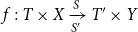 $f:T \times X\xrightarrow [S']{S}{T'\times Y}$
be a 2-cell in
 $Dbl(\mathbb{C})$
. The value-to-state conversion of
 $f$
at
 $(T, T')$
is another 2-cell, denoted
 ${}^{T}\lfloor{f}\rceil _{T'}$
, with the same underlying morphism but different source and target 1-cells:
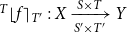 ${}^{T}\lfloor{f}\rceil _{T'}:X\xrightarrow [S'\times T']{S\times T}Y$
.
Equalities satisfied by delayed trace operator.

When the objects
 $(T, T')$
involved in the conversion are clear from context, we drop them from the notation and write
 $\lfloor{f}\rceil$
for
 ${}^{T}\lfloor{f}\rceil _{T'}$
.
The value-to-state conversion is depicted inside the tile:

The pointwise application of this operation to all the 2-cells in a stateful morphism sequence is the delayed trace operator.
Definition 18.
Suppose
 $(i,\textbf{s}):\textbf{T}\times \textbf{X}\to \mathop{\bigcirc }{\textbf{T}}\times \textbf{Y}$
is a morphism in
 $\mathrm{St}(\mathbb{C})$
. (Recall
 $\mathop{\bigcirc }{\textbf{T}}=[\textbf{T}_{\bullet + 1}]$
.) The delayed trace of
 $\textbf{s}$
along
 $\textbf{T}$
with an initial state
 $p:1\rightarrow \textbf{T}_0$
is the following morphism in
 $\mathrm{St}(\mathbb{C})(\textbf{X}, \textbf{Y})$
:
 \begin{align*} {\mathrm{tr}}_{p}^{\textbf{T}}{(i, \textbf{s})} \mathbin{\triangleq } (\langle i, p\rangle, [{}^{\textbf{T}_\bullet }\lfloor{\textbf{s}_\bullet }\rceil _{\textbf{T}_{\bullet +1}}]). \end{align*}
Note this operation is well defined on extensional equivalence classes of stateful morphism sequences and therefore is an operation on
 $\mathrm{St}(\mathbb{C})$
morphisms. The delayed trace of
 $\mathrm{St}(\mathbb{C})$
already differs from the standard monoidal trace in two ways: first, the domain and codomain types that are bound (
 $\textbf{T}$
and
 $\mathop{\bigcirc }\textbf{T}$
) do not match, and second, the delayed trace also requires a designated global element
 $p$
called the initial state. Despite these differences, many of the trace axioms holds for the delayed trace operator.
Proposition 19.
Suppose
 $(i,\textbf{s}): \textbf{T}\times \textbf{X}\rightarrow \mathop{\bigcirc }{\textbf{T}}\times \textbf{Y}$
is a morphism in
 $\mathrm{St}(\mathbb{C})$
. Suppose
 $(h,\textbf{r}): \textbf{Y}\to \textbf{Z}$
,
 $(j,\textbf{t}): \textbf{W}\to \textbf{X}$
and
 $(f,\textbf{p}): \textbf{W}\to \textbf{Z}$
are other arbitrary morphisms in
 $\mathrm{St}(\mathbb{C})$
. Five standard axioms of monoidal trace, presented in Figure 7, hold of delayed trace.
The yanking axiom of the trace operator fails for the delayed trace operator. Consider the symmetry morphism
 $\sigma _{\textbf{X},\mathop{\bigcirc }\textbf{X}}:\textbf{X}\times \mathop{\bigcirc }\textbf{X}\rightarrow \mathop{\bigcirc }\textbf{X}\times \textbf{X}$
in
 $\mathrm{St}(\mathbb{C})$
. Define its delayed trace with an initial state
 $i:1\rightarrow \textbf{X}_0$
to be
 \begin{equation*}r_{\textbf {X}}(i)\mathbin {\triangleq }\mathop {\mathrm {tr}}\nolimits ^{\textbf {X}}_{i}(\sigma _{\textbf {X},\mathop {\bigcirc }\textbf {X}}):\mathop {\bigcirc }\textbf {X}\rightarrow \textbf {X}\end{equation*}
To get a better understanding of
 $r_{\textbf{X}}(i)$
, we first draw the value-to-state conversion in a single 2-cell in this morphism.

Doing value-to-state conversion along the whole sequence
 $\sigma _{\textbf{X}, \mathop{\bigcirc }\textbf{X}}$
and supplying the initial value
 $i: 1 \to \textbf{X}_0$
yields:

We can see that the input at clock tick
 $k$
is output at clock tick
 $k+1$
. Therefore, instead of the identity, which is what
 $r_{\textbf{X}}(i)$
would be if the yanking axiom held, we have a morphism that operates as a delay gate.
The dinaturality axiom of the trace operator also fails for the delayed trace operator. Dinaturality corresponds to sliding circuits from one end of a feedback loop to the other, but doing so with a delay gate in the loop affects the gate’s initial state. In digital circuit design, this kind of operation is called retiming (Leiserson and Saxe, Reference Leiserson and Saxe1991), and initial states of registers is a delicate issue in this subject. The delayed trace operator satisfies the following modified dinaturality property:
Theorem 20.
Suppose
 $(i,\textbf{s}):\textbf{T}\times \textbf{X}\rightarrow \mathop{\bigcirc }{\textbf{U}}\times \textbf{Y}$
and
 $(j,\textbf{g}):\textbf{U}\rightarrow \textbf{T}$
are morphisms in
 $\mathrm{St}(\mathbb{C})$
. For any
 $u:1\rightarrow \textbf{U}_0$
,
 \begin{align*} \mathop{\mathrm{tr}}\nolimits ^{\textbf{U}}_{u}(((j,\textbf{g})\times \textbf{X})\circ (i,\textbf{s})) =\mathop{\mathrm{tr}}\nolimits ^{\textbf{T}}_{u^{\prime}}((i,\textbf{s})\circ ((j',\mathop{\bigcirc }\textbf{g})\times \textbf{Y})) \end{align*}
where
 $\langle j', u' \rangle = U\textbf{g}_0\circ \langle j,u\rangle$
.
Proof. Let
 $r_i = \lfloor{({\textrm{id}}_{Y_i}^h \times g_i)* s_i}\rceil$
. By induction, obtain the equality of this:
 \begin{equation} U(r_0;\; \cdots ;\; r_n) \circ ({\textrm{id}}_{S_{n+1}\times \prod ^n Y_i}\times \sigma _{T_{n+1},U_{n+1}}) \end{equation}
and this:
 \begin{equation} U(t_0;\cdots ; t_n) \circ ({\textrm{id}}_{\prod ^n Y_i}\times U(g_n)\times{\textrm{id}}_{T_{n+1}}). \end{equation}
Then observe the
 $n$
th truncation of
 $(r_i)$
is (5) followed by
 $\pi _{\prod ^n Y_i}$
and similarly, the
 $n$
th truncation of
 $(t_i)$
is (6) followed by the same projection. Therefore, they are observationally equivalent, though not equal as sequences.
A special case of this modified dinaturality is an abstract version of circuit retiming, which allows us to commute properly initialized delay gates and stateless morphisms.
Corollary 21.
For any
 $\textbf{f}:\textbf{X}\rightarrow \textbf{Y}$
in
 $\mathbb{C}^{\mathbb{N}}$
, and initial state
 $i:1\rightarrow \textbf{X}_0$
, we have
 $H\textbf{f}\circ r_{\textbf{X}}(i)=$
 $r_{\textbf{Y}}(\textbf{f}_0\circ i)\circ H(\mathop{\bigcirc } \textbf{f})$
.
The following representation result says that every morphism in
 $\mathrm{St}(\mathbb{C})$
can be obtained as the delayed trace of a stateless morphism.
Theorem 22.
For any morphism
 $(i,\textbf{s})$
in
 $\mathrm{St}(\mathbb{C})$
, the following equality holds:
 \begin{align*} (i,\textbf{s})= {\mathrm{tr}}_{i}^{\mathrm{st}(i,\textbf{s})} (H[U(\textbf{s}_\bullet )]) \end{align*}
This theorem is our formalization of Folklore knowledge that every synchronous digital circuit can be written as a single combinational (stateless) circuit plus a feedback loop with a register.
5.1 Delayed trace in
$\mathrm{St}_0(\mathbb{C})$

The category
 $\mathrm{St}_0(\mathbb{C})$
is also closed under the delayed trace operator. Since
 $\textbf{X} = \mathop{\bigcirc } \textbf{X}$
in
 $\mathrm{St}_0(\mathbb{C})$
, delayed dinaturality is even closer to true dinaturality.
Corollary 23.
Suppose
 $(i,[s]):[T]\times [X]\rightarrow [U]\times [Y]$
is a morphism in
 $\mathrm{St}_0(\mathbb{C})$
, and
 $(j,[g]):[U]\rightarrow [T]$
is another morphism in
 $\mathrm{St}_0(\mathbb{C})$
. For any initial state
 $u:1\rightarrow U$
,
 \begin{align*} &\mathop{\mathrm{tr}}\nolimits ^{[U]}_{u}(((j,[g])\times{\textrm{id}}_{[X]})\circ (i,[s]))\\ &=\mathop{\mathrm{tr}}\nolimits ^{[T]}_{u'}((i,[s])\circ ((j',[g])\times{\textrm{id}}_{[Y]})) \end{align*}
where
 $\langle j', u' \rangle = g\circ \langle j,u\rangle$
.
Corollary 24.
For any
 $f:X\rightarrow Y$
in
 $\mathbb{C}$
, and initial state
 $i:1\rightarrow X$
, we have
 $H[f]\circ r_{[X]}(i)=r_{[Y]}(f\circ i)\circ H([f])$
.
5.2 Diagrammatic reasoning about
$\mathrm{St}_0(\mathbb{C})$
morphisms

Here, we informally introduce a diagrammatic syntax for morphisms in
 $\mathrm{St}_0(\mathbb{C})$
. Theorem22 indicates that we can generate all
 $\mathrm{St}_0(\mathbb{C})$
morphisms with the following grammar:
 \begin{equation*}\varphi ::= H_0f \,|\, \varphi _1\circ \varphi _2 \,|\, \varphi _1\times \varphi _2 \,|\, \mathop {\mathrm {tr}}\nolimits ^{\textbf {S}}_{i}(\varphi )\end{equation*}
where
 $f$
is a
 $\mathbb{C}$
-morphism. We generate circuit diagrams with a parallel 2-dimensional grammar:

where the box labeled
 $H_0f$
has
 $m$
inputs and
 $n$
outputs when
 $f: \prod _{k = 1}^m A_k \rightarrow \prod _{k=1}^n B_k$
. As is typical in string diagrams,
 $H_0{\textrm{id}}_X$
is depicted by a wire and
 $H_0\sigma _{X,Y}$
by a wire crossing. Additionally, we depict
 $H_0!_A$
and
 $H_0\langle{\textrm{id}}_A,{\textrm{id}}_A \rangle$
with a discarder and copier:

The evident interpretation in
 $\mathrm{St}_0(\mathbb{C})$
of these diagrams induces an equivalence on the diagrams. For instance, as a special case of Corollary 23, sliding a stateless node along a loop is possible by changing the value in the delay gate:

As an example of diagrammatic reasoning, we show that this simple delayed dinaturality plus superposing allows us to obtained delayed dinaturality for stateful circuits (Theorem20).

More formal treatment of this diagrammatic equational system can be done through the construction of the free cartesian category with the delayed trace operator. We reserve the formal axiomatization of general delayed trace operators and free categories with these structures for future work and move on to the study of the differentiability of the causal computations realized by
 $\mathrm{St}(\mathbb{C})$
.
6. Cartesian Differential Structure
In this section, we investigate differentiation in
 $\mathrm{St}(\mathbb{C})$
. Our primary tool is the theory of Cartesian differential categories, introduced by Blute et al. (Reference Blute, Cockett and Seely2009). We begin by recalling background.
Definition 25 (Blute et al. (Reference Blute, Cockett and Seely2009)). A left additive category is a Cartesian category such that every object has a designated commutative monoid structure, which we write
 $+_X: X\times X \to X$
and
 $0_X: 1 \to X$
. These commutative monoids must be compatible with the Cartesian structure of the category by satisfying
 $0_{X\times Y} = 0_X \times 0_Y$
and
 $+_{X\times Y} = (+_X \times +_Y)\circ (X\times \sigma _{Y,X}\times Y)$
.
The vector space structure on Euclidean spaces is a classic example of left additive structure.
Example 1 (Blute et al. (Reference Blute, Cockett and Seely2009)). The category
 $\textbf{Euc}_\infty$
, whose objects are
 ${\mathbb{R}}^n$
for
 $n \geq 0$
and morphisms are smooth functions, is a left additive category where
 $+_{{\mathbb{R}}^n}$
is the sum of vectors in
 ${\mathbb{R}}^n$
and
 $0_{{\mathbb{R}}^n}$
is the zero vector in
 ${\mathbb{R}}^n$
.
To obtain left additive structure for
 $\mathrm{St}(\mathbb{C})$
, it suffices to take sequences of the corresponding pieces of left additive structure for
 $\mathbb{C}$
, much like how the Cartesian structure of
 $\mathbb{C}$
lifted.
Lemma 26.
If
 $\mathbb{C}$
is a left additive category, so is
 $\mathrm{St}(\mathbb{C})$
.
Proof. We already know
 $\mathbb{C}$
being Cartesian implies
 $\mathrm{St}(\mathbb{C})$
is Cartesian. A commutative monoid structure on
 $\textbf{X}$
is given by componentwise monoid structure:
 $+_{\textbf{X}} \mathbin{\triangleq } [+_{\textbf{X}_\bullet }:\textbf{X}_\bullet \times \textbf{X}_\bullet \xrightarrow [1]{1}\textbf{X}_\bullet ]$
and
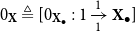 $0_{\textbf{X}}\mathbin{\triangleq } [0_{\textbf{X}_\bullet }:1\xrightarrow [1]{1}\textbf{X}_\bullet ]$
.
Next, we introduce some helpful families of morphisms present in every Cartesian left additive category that are useful for condensing later definitions.
Definition 27.
Let
 $\mathbb{C}$
be a Cartesian left additive category. For every object
 $X$
from
 $\mathbb{C}$
[or pair of objects
 $(X, Y)$
], let
-
•
$\delta _{X,Y} \mathbin{\triangleq } X \times \sigma _{Y, X} \times Y$
-
•
$\alpha _X \mathbin{\triangleq } \delta _{X, X} \circ (X \times X\times \Delta _X)$
-
•
$\beta _X \mathbin{\triangleq } X\times{!_{X}} \times X\times X$
-
•
$\gamma _{X,Y} \mathbin{\triangleq } (X\times \Delta _X\times Y \times Y) \circ \delta _{X,Y}$
-
•
$\zeta _X \mathbin{\triangleq } X\times 0_{X\times X} \times X$





Now we are ready to describe the central object of our study this section, Cartesian differential categories.
Definition 28.
A Cartesian differential category is a left additive category
 $\mathbb{C}$
with a Cartesian differential operator
 $D: \mathbb{C}(X, Y) \to \mathbb{C}(X\times X, Y)$
, satisfying:
-
CD1.
$Ds = s\times{{!_{\mathop{\mathrm{dom}} (s)}}}$
for
$s \in \{X, \sigma _{X,Y},{!_{X}}, \Delta _X, +_X, 0_X\}$
-
CD2.
$Df\circ (0_X \times X) = 0_Y \circ{!_{X}}$
-
CD3.
$Df \circ (+_X\times X) = +_Y\circ (Df\times Df)\circ \alpha _X$
-
CD4.
$D(g\circ f) = Dg \circ (Df \times f) \circ (X \times \Delta _X)$
-
CD5.
$D(f\times h) = (Df \times Dh)\circ \delta _{X,V}$
-
CD6.
$DDf\circ \zeta _X = Df$
-
CD7.
$DDf\circ \delta _{X,X} = DDf$








for all
 $f: X \to Y$
,
 $g: Y \to Z$
, and
 $h: V \to W$
.
This definition of a Cartesian differential category is not exactly that of Blute et al. (Reference Blute, Cockett and Seely2009), but it is mostly straightforward to check that they are equivalent. The biggest changes are in axioms CD6 and CD7, for which we have taken alternate forms given in Cockett and Cruttwell (Reference Cockett and Cruttwell2014) (Proposition 4.2).
Example 2 (Blute et al. (Reference Blute, Cockett and Seely2009)).
 $\textbf{Euc}_\infty$
is a Cartesian differential category. The differential operator
 $D$
sends a smooth function
 $f:{\mathbb{R}}^n \to{\mathbb{R}}^m$
to
 $Df: (x_1, x_2) \mapsto Jf|_{x_2}\times x_1$
, where
 $Jf|_{x_2}$
is the Jacobian matrix of
 $f$
evaluated at
 $x_2$
.
In light of the standard example, we can describe the ideas behind the CD axioms. CD1 says that the basic morphisms provided by the structure of the Cartesian left additive category are their own derivatives (i.e.
 $Js|_{x_2}\times x_1 = s(x_1)$
), while CD2 and CD3 express the fact that
 $Jf|_{x_2}\times x_1$
is linear in its
 $x_1$
argument. CD4 is the chain rule, while CD5 says the derivative of a parallel composition is the parallel composition of derivatives. CD6 and CD7 have to do with partial derivatives: CD7 is the symmetry of partial derivatives, and CD6 is trickier to describe exactly but is related to the linearity of partial derivatives.
Many of the CD axioms mention the parallel composition of morphisms. When we state these in
 $\mathrm{St}(\mathbb{C})$
, it will be helpful to have an operation for forming parallel compositions. This motivates us to define the following operation on 2-cells.
Definition 29.
Let
 $f:X\xrightarrow [S']{S} Y$
and
 $k:Z\xrightarrow [T']{T} W$
be arbitrary 2-cells from
 $Dbl(\mathbb{C})$
. The cross-composition of
 $f$
and
 $k$
is another 2-cell
 $f\boxtimes k:X\times Z\xrightarrow [S'\times T']{S\times T}Y\times W$
defined by:
 \begin{equation*}f\boxtimes k = ({}^{T}\lfloor {(T\times Y)^h}\rceil _{T};\; k)*(f;\; {}^{S'}\lfloor {(S'\times Z)^h}\rceil _{S'}).\end{equation*}
It may be easier to understand cross-composition by its underlying morphism:

The idea of this operation is to execute two 2-cells in parallel, without their states or values interacting with each other. We are purposefully avoiding using
 $\times$
for
 $\boxtimes$
so as not to imply there is some kind of Cartesian structure on the double category
 $Dbl(\mathbb{C})$
.
To avoid using too many grouping symbols when disambiguating 2-cell expressions involving
 $;$
,
 $*$
, and
 $\boxtimes$
, we will say
 $\boxtimes$
binds tightest, then
 $;$
, and last
 $*$
, so
 $f;\; g \boxtimes h * k$
means
 $(f;\; (g \boxtimes h)) * k$
.
As desired, this operation implements Cartesian product in
 $\mathrm{St}(\mathbb{C})$
.
Lemma 30.
 $(i, \textbf{f})\times (j, \textbf{g}) = (\langle i, j \rangle, [{\textbf{f}}_\bullet \boxtimes{\textbf{g}}_\bullet ])$
for all
 $\mathrm{St}(\mathbb{C})$
morphisms
 $(i, \textbf{f})$
and
 $(j, \textbf{g})$
.
We can now start defining the Cartesian differential operator on
 $\mathrm{St}(\mathbb{C})$
. For the remainder of this section, we assume
 $\mathbb{C}$
is a Cartesian differential category and let
 $D$
be its differential operator. We start by defining our differential operator within a time step, by giving some operations on 2-cells.
Definition 31.
We define two endofunctions on 2-cells from
 $Dbl(\mathbb{C})$
. The first,
 $\mathscr{D}_0$
, takes the 2-cell
 $f:X\xrightarrow [S']{S} Y$
to the 2-cell
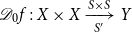 $\mathscr{D}_0 f:X\times X\xrightarrow [S']{S\times S}Y$
with
 $U\mathscr{D}_0 f \triangleq DUf \circ \delta _{S, X}$
.
The second,
 $\mathscr{D}$
, takes
 $f$
to
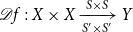 $\mathscr{D} f:X\times X\xrightarrow [S'\times S']{S\times S}Y$
with
 \begin{equation*}\mathscr {D} f \mathbin {\triangleq } (S\times \Delta _S)^v;\; (\mathscr {D}_0 f \boxtimes ({!_{Y}}^h *f)) * (X\times \Delta _X)^h.\end{equation*}
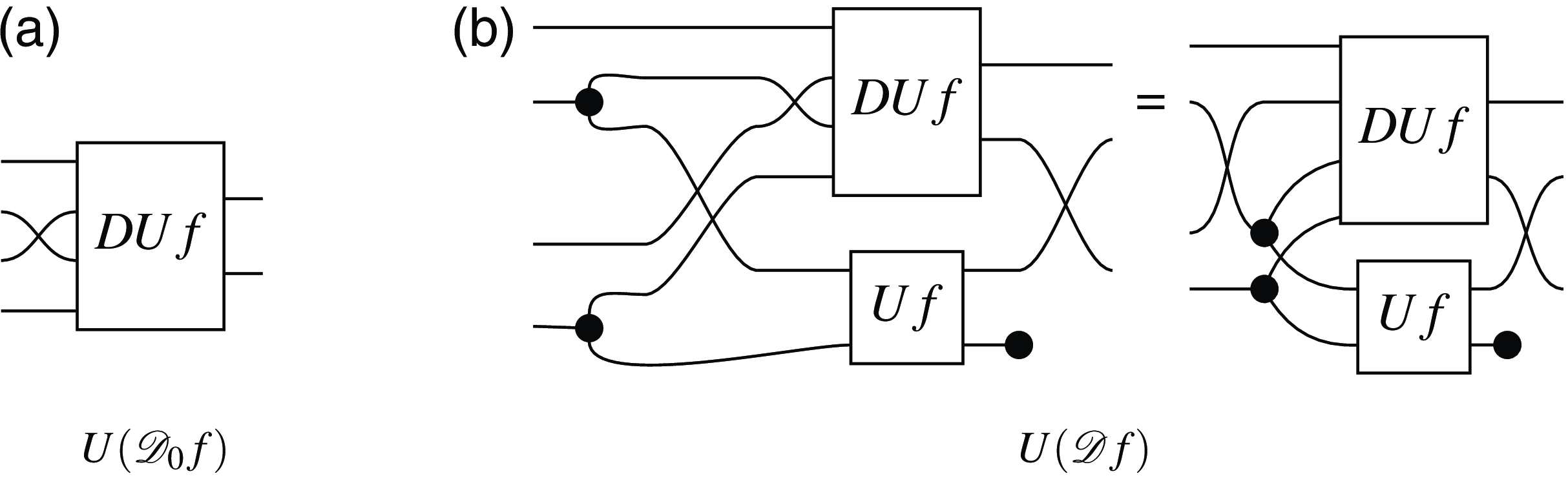
The string diagrams for the underlying morphisms of
 $\mathscr{D}_0$
and
 $\mathscr{D}$
may be easier to understand; these are shown in Figure 8.
Underlying morphisms for Definition 31.

The Cartesian differential operator on
 $\mathrm{St}(\mathbb{C})$
is based on
 $\mathscr{D}$
, and so to prove that it is a differential operator, we need some properties of
 $\mathscr{D}$
.
Proposition 32.
Let
 $f:X\xrightarrow [S']{S} Y$
,
 $g:Y\xrightarrow [T']{T} Z$
,
 $h:Z\xrightarrow [S'']{S'} W$
, and
 $k:Z\xrightarrow [T']{T} W$
be arbitrary 2-cells. The following are properties of
 $\mathscr{D}$
:
-
1. If
$\varphi \in \mathbb{C}(X, Y)$
, then
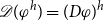
$\mathscr{D}(\varphi ^h) = (D\varphi )^h$
and
$\mathscr{D}(\varphi ^v) = ((D\varphi \times \varphi )\circ (X\times \Delta _X))^v$
. -
2.
$(0_S\times S)^v;\; \mathscr{D} f * (0_X \times X)^h = (0_Y \circ !_Y)^h * f;\; (0_{S'} \times S')^v$
-
3.
$(+_S\times S)^v;\; \mathscr{D} f * (+_X \times X)^h = \alpha _S^v;\;(+_Y^h * \mathscr{D} f \boxtimes \mathscr{D} f * \alpha _X^h);\; \beta _{S'}^v ;\; (+_{S'}\times S')^v$
-
4.
$\mathscr{D}(f;\; h) = (\mathscr{D} f;\; \mathscr{D} h) * \delta _{X,Z}^h$
-
5.
$\mathscr{D}(g* f);\; \gamma _{S', T'}^v = \gamma _{S, T}^v;\; (\mathscr{D} g * (\mathscr{D} f \boxtimes f)* (X\times \Delta _X)^h)$
-
6.
$\mathscr{D}(f \boxtimes k);\; \delta _{S', T'}^v = \delta _{S, T}^v;\; \mathscr{D} f \boxtimes \mathscr{D} k * \delta _{X, Z}^h$
-
7.
$\zeta _S^v;\; \mathscr{D} \mathscr{D} f * \zeta _X^h = \mathscr{D} f;\; \zeta _{S'}^v$
-
8.
$\delta _{S,S}^v;\; \mathscr{D} \mathscr{D} f * \delta _{X, X}^h = \mathscr{D} \mathscr{D} f;\; \delta _{S', S'}^h$









Proof. The method to prove these properties is conceptually simple: use the definitions of the operations on 2-cells (and properties of left additive categories and CD axioms) to check that both sides of each equation have (1) the same boundary 1-cells and (2) the same underlying
 $\mathbb{C}$
-morphism.
Checking (1), namely that the source and target 1-cells of the 2-cells on each side of each of these eight equations match, is straightforward. Checking (2) is not an effortless task; we have two kinds of composition and will be making heavy use of the axioms of Cartesian differential operators. We find it easiest to do this reasoning with string diagrams, so this is what we will present here.
Throughout this proof, let
 $Uf = \phi$
,
 $Ug = \psi$
,
 $Uh = \xi$
, and
 $Uk = \kappa$
.
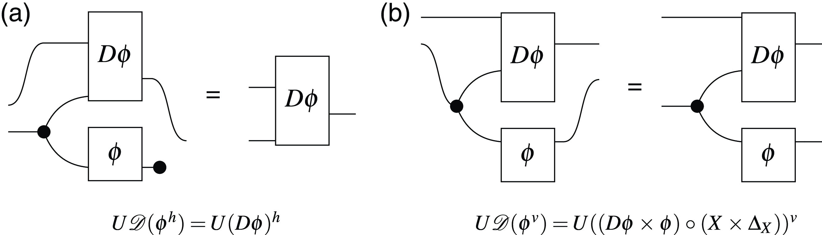
Property 1: If
 $\phi \in \mathbb{C}(X, Y)$
, then
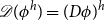 $\mathscr{D}(\phi ^h) = (D\phi )^h$
and
 $\mathscr{D}(\phi ^v) = ((D\phi \times \phi )\circ (X\times \Delta _X))^v$
.
When
 $\phi$
is oriented horizontally, it has no state. This simplifies the diagram for the underlying morphism of
 $\mathscr{D}$
(from Figure 8b) considerably; properties of copy-discard show this is equal to the underlying morphism of
 $(D\phi )^h$
. When
 $\phi$
is oriented vertically, it has no values. Omitting the value portion of
 $U\mathscr{D} f$
yields the left side of Figure 9b which is exactly
 $(D\phi \times \phi )\circ (X\times \Delta _X)$
.
String diagrams for property 1.

Property 2:
 $(0_S\times S)^v;\; \mathscr{D} f * (0_X \times X)^h = (0_Y \circ !_Y)^h * f;\; (0_{S'} \times S')^v$
From Lemma 3 and the diagram for the underlying morphism of
 $\mathscr{D} f$
,

where the middle equality is by the CD2 axiom for
 $D$
.
Property 3:
 $(+_S\times S)^v;\; \mathscr{D} f * (+_X \times X)^h = \alpha _S^v;\;(+_Y^h * \mathscr{D} f \boxtimes \mathscr{D} f * \alpha _X^h);\; \beta _{S'}^v ;\; (+_{S'}\times S')^v$
We start from the right-hand side of this equation. To aid parsing this complicated string diagram, we draw a red box around parts of the diagram to serve as a label. Everything in red has no mathematical meaning—it is only there for aid of understanding.

In the first step, we have used properties of copying and discarding to eliminate the middle
 $\phi$
morphism, preceding copies, and succeeding discards. In the next step, we use properties of monoidal categories and properties of copying to rearrange, so the boxed region is the left-hand side of CD3 (
 $+_{S'\times Y} \circ (D\phi \times D\phi ) \circ \alpha _{S\times X}$
). In the final step, we use CD3 and further monoidal category properties.
Property 4:
 $\mathscr{D}(f;\; h) = (\mathscr{D} f;\; \mathscr{D} h) * \delta _{X,Z}^h$
.
Using the CD axioms for
 $D$
, we compute the differential of the underlying morphism of
 $f;\; h$
, then do some simplification:

We use that result to construct a string diagram for
 $U\mathscr{D}(f; h)$
:

In the first step, we use properties of monoidal categories to rearrange the composition. The second step uses naturality of the copy to eliminate a
 $\phi$
, along with further monoidal rearrangements. At this point, the underlying morphisms for
 $\mathscr{D} f$
and
 $\mathscr{D} h$
have appeared, so we substitute these in the next step. Finally, we use the definition of vertical composition and arrive at the string diagram of
 $U((\mathscr{D} f;\; \mathscr{D} h) * \delta _{X,Z}^h)$
(cf. Lemma 3).
Property 5:
 $\mathscr{D}(g* f);\; \gamma _{S', T'}^v = \gamma _{S, T}^v;\; (\mathscr{D} g * (\mathscr{D} f \boxtimes f)* (X\times \Delta _X)^h)$
.
Using the CD axioms for
 $D$
, we compute the differential of the underlying morphism of
 $g* f$
:

We use that result to construct a string diagram for
 $U(\mathscr{D}(g* f);\; \gamma _{S', T'}^v)$
:

In the first row, we make extensive use of properties of copy-discard monoidal categories to realize the underlying morphisms of
 $\mathscr{D} g$
and
 $\mathscr{D} f$
(hinted in red). In the next two steps, we substitute these into the diagram. The final step in the second row is a monoidal rearrangement which finds the underlying morphism of
 $\mathscr{D} f \boxtimes f$
(again in red) by definition of
 $\boxtimes$
. Then using the definition of horizontal composition in the last step, we obtain the string diagram of
 $U(\gamma _{S, T}^v;\; (\mathscr{D} g * (\mathscr{D} f \boxtimes f))* (X\times \Delta _X)^h)$
.
Property 6:
 $\mathscr{D}(f \boxtimes k);\; \delta _{S', T'}^v = \delta _{S, T}^v;\; \mathscr{D} f \boxtimes \mathscr{D} k * \delta _{X, Z}^h$
.
Using the CD axioms for
 $D$
, we compute the differential of the underlying morphism of
 $f\boxtimes k$
:

We use that result to construct a string diagram for
 $U(\mathscr{D}(f \times k);\; \delta _{S', T'}^v)$
:

This only requires some rearrangement using axioms of monoidal categories to obtain the string diagram for the underlying morphism of
 $\delta _{S, T}^v;\; \mathscr{D} f \boxtimes \mathscr{D} k * \delta _{X, Z}^h$
.
For the next two properties, we need the underlying morphism for
 $\mathscr{D}\mathscr{D} f$
. Using the definition of
 $\mathscr{D}$
and the axioms of CDCs, one can show
 $U\mathscr{D} \mathscr{D} f$
is given by the diagram.

Property 7:
 $\zeta _S^v;\; \mathscr{D} \mathscr{D} f * \zeta _X^h = \mathscr{D} f;\; \zeta _{S'}^v$
.

In the first step, we use the naturality of the copy morphisms to distribute zero maps to the appropriate places in the diagram. In the next step, we use CD2 for
 $D$
twice. Finally, in the last step, we clean up some discarded copies and use CD6 for
 $D$
to simplify
 $DD\phi \circ \zeta _{S\times X}$
.
Property 8:
 $\delta _{S,S}^v;\; \mathscr{D} \mathscr{D} f * \delta _{X, X}^h = \mathscr{D} \mathscr{D} f;\; \delta _{S', S'}^h$
.

The first step involves properties of cartesian categories, both in swapping the order of the two
 $D\phi$
morphisms and also in reassociating the copying. In the second step, the swapping before
 $DD\phi$
is undone by invoking CD7 for
 $D$
.
An important consequence of Proposition 32(4) is the following extension to finite sequences of vertically composed 2-cells.
Lemma 33.
Let
 $(f_k)_{k=0}^n$
be a finite sequence of vertically composable 2-cells. Then
 $\mathscr{D}(f_0 ;\cdots ; f_n) = (\mathscr{D} f_0 ;\cdots ;\mathscr{D} f_n)* z^h$
, where
 $z$
is the unzipping isomorphism in
 $\mathbb{C}$
of type
 \begin{align*} \textstyle \prod _{k=0}^n(\mathop{\mathrm{dom}} f_k\times \mathop{\mathrm{dom}} f_k) \rightarrow (\prod _{k=0}^n\mathop{\mathrm{dom}} f_k)\times (\prod _{k=0}^n\mathop{\mathrm{dom}} f_k). \end{align*}
We can now state the operator we seek on
 $\mathrm{St}(\mathbb{C})$
.
Definition 34.
The componentwise application of
 $\mathscr{D}$
to 2-cells in a
 $\mathrm{St}(\mathbb{C})$
morphism,
 $\mathscr{D}^*: (i, \textbf{s}) \mapsto (\langle 0, i \rangle, [\mathscr{D}{\textbf{s}}_\bullet ])$
, is a well-defined operation on
 $\mathrm{St}(\mathbb{C})$
morphisms of type
 \begin{equation*}\mathscr {D}^*: \mathrm {St}(\mathbb{C})(\textbf {X}, \textbf {Y}) \to \mathrm {St}(\mathbb{C})(\textbf {X}\times \textbf {X}, \textbf {Y}).\end{equation*}
To justify this definition, we must immediately check this operation is well defined on stateful morphism sequences.
Lemma 35.
 $\mathscr{D}^*$
is well defined.
Proof. Let
 $(i, \textbf{s})$
and
 $(j, \textbf{t})$
be extensionally equivalent sequences. We must show
 $(\mathscr{D} i, [\mathscr{D}{\textbf{s}}_\bullet ])$
and
 $(\mathscr{D} j, [\mathscr{D}{\textbf{t}}_\bullet ])$
are extensionally equivalent.
 \begin{eqnarray*} \mathscr{D} i ;\; \mathscr{D}\textbf{s}_0 ;\ldots ; \mathscr{D}\textbf{s}_n ;\; d_{(\mathop{\mathrm{nxt}} s_n)^2} &=& \mathscr{D} i ;\; \mathscr{D}\textbf{s}_0 ;\ldots ; \mathscr{D}\textbf{s}_n ;\; \mathscr{D} d_{\mathop{\mathrm{nxt}} s_n} \\ &=& \mathscr{D}(i ;\textbf{s}_0 ;\ldots ;\textbf{s}_n ;\; d_{\mathop{\mathrm{nxt}} s_n}) * z^{-1} \\ &=& \mathscr{D}(j ;\;\textbf{t}_0 ;\ldots ;\;\textbf{t}_n ;\; d_{\mathop{\mathrm{nxt}} t_n}) * z^{-1} \\ \end{eqnarray*}
where the first line is by Proposition 32(2), the second by Lemma 33, and the last by the fact that
 $(i, \textbf{s})$
and
 $(j, \textbf{t})$
are extensionally equivalent. Here, it is crucial that extensionally equivalent sequences have the same source values so that the
 $z$
obtained from Lemma 33 when
 $\varphi = \textbf{s}$
matches the
 $z$
obtained when
 $\varphi = \textbf{t}$
. The proof then finishes by reversing the first two steps.
A key contribution of this work is the fact that this operation is actually a Cartesian differential operator.
Theorem 36.
 $\mathscr{D}^*$
is a Cartesian differential operator.
The strategy for this proof is to use the properties of
 $\mathscr{D}$
from Proposition 32, which were selected to be used with the Shim Lemma to obtain the CD axioms. For example, in this context, CD4 (the chain rule) states:
 \begin{equation*}\mathscr {D}^* ((j, \textbf {g})\circ (i, \textbf {f})) = \mathscr {D}^*(j, \textbf {g})\circ (\mathscr {D}^*(i, \textbf {f})\times (i, \textbf {f}))\circ (\textbf {X} \times \Delta _{\textbf {X}}).\end{equation*}
The key step in proving this is invoking the Shim Lemma with
 ${\textbf{b}}_\bullet = \gamma _{{\textbf{S}}_\bullet, {\textbf{T}}_\bullet }$
. We have two conditions to check for this invocation:
 $\gamma _{\textbf{S}_0, \textbf{T}_0}\circ \langle 0_{\textbf{S}_0}, 0_{\textbf{T}_0}, i, j \rangle = \langle 0_{\textbf{S}_0}, i, i, 0_{\textbf{T}_0}, j \rangle$
and
 \begin{align*} \mathscr{D}({\textbf{g}}_\bullet *{\textbf{f}}_\bullet );\; \gamma _{\textbf{S}_{\bullet +1},\textbf{T}_{\bullet +1}}^v = \gamma _{{\textbf{S}}_\bullet, {\textbf{T}}_\bullet }^v;\; (\mathscr{D}{\textbf{g}}_\bullet * (\mathscr{D}{\textbf{f}}_\bullet \boxtimes{\textbf{f}}_\bullet )* ({\textbf{X}}_\bullet \times \Delta _{{\textbf{X}}_\bullet })^h), \end{align*}
the latter of which is a case of Proposition 32(5).
We can now prove CD4 for
 $\mathscr{D}^*$
:
 \begin{align*} \mathscr{D}^*(&(j, \textbf{g}) \circ (i, \textbf{f})) = (\langle 0_{\textbf{S}_0}, 0_{\textbf{T}_0}, i, j \rangle, [\mathscr{D}({\textbf{g}}_\bullet *{\textbf{f}}_\bullet )]) \\ &= (\langle 0_{\textbf{S}_0}, i, i, 0_{\textbf{T}_0}, j \rangle, [\mathscr{D}{\textbf{g}}_\bullet * (\mathscr{D}{\textbf{f}}_\bullet \boxtimes{\textbf{f}}_\bullet )* ({\textbf{X}}_\bullet \times \Delta _{{\textbf{X}}_\bullet })^h]) \\ &= \mathscr{D}^*(j, \textbf{g})\circ (\mathscr{D}^*(i, \textbf{f}) \times (i, \textbf{f})) \circ (\textbf{X}\times \Delta _{\textbf{X}}) \end{align*}
where the second line is the Shim Lemma step.
Proof. We show that
 $\mathscr{D}^*$
satisfies the seven axioms given in Definition 28. Most of the hard work has already been done in Proposition 32; we use the properties of
 $\mathscr{D}$
established there in concert with the Shim Lemma to obtain most of the CD axioms.
Let
 $f = (i, \textbf{f}): \textbf{X} \to \textbf{Y}$
,
 $g = (j, \textbf{g}): \textbf{Y} \to \textbf{Z}$
and
 $h = (\ell, \textbf{h}): \textbf{Z} \to \textbf{W}$
. Let
 $\textbf{S}$
,
 $\textbf{T}$
, and
 $\textbf{U}$
be the state sequences of
 $f$
,
 $g$
, and
 $h$
, respectively.
-
CD1.
$\mathscr{D}^* s = s\times{{!_{\mathop{\mathrm{dom}} (s)}}}$
for
$s \in \{\textbf{X}, \sigma _{\textbf{X},\textbf{Y}},{!_{\textbf{X}}}, \Delta _{\textbf{X}}, +_{\textbf{X}}, 0_{\textbf{X}}\}$
. These
$s$
are of the form
$({\textrm{id}}_1, [({\textbf{s}}_\bullet )^h])$
where each
${\textbf{s}}_\bullet$
is a
$\mathbb{C}$
-morphism from
$\{X, \sigma _{X,Y},{!_{X}}, \Delta _X, +_X, 0_X\}$
. Therefore,where the last step in the first line is by Proposition 32(1), and the first step in the second line is by CD1 for
\begin{align*} \mathscr{D}^* s &= \mathscr{D}^*({\textrm{id}}_1, [({\textbf{s}}_\bullet )^h]) = ({\textrm{id}}_1, [\mathscr{D}({\textbf{s}}_\bullet )^h]) = ({\textrm{id}}_1, [(D{\textbf{s}}_\bullet )^h]) \\ & = (\langle{\textrm{id}}_1,{\textrm{id}}_1 \rangle, [({\textbf{s}}_\bullet \times{!_{\mathop{\mathrm{dom}}{{\textbf{s}}_\bullet }}})^h]) = ({\textrm{id}}_1, [({\textbf{s}}_\bullet )^h]) \times ({\textrm{id}}_1, [({!_{\mathop{\mathrm{dom}}{{\textbf{s}}_\bullet }}})^h]) = s \times{!_{\mathop{\mathrm{dom}} s}} \end{align*}
$D$
.
-
CD2.
$\mathscr{D}^* (i, \textbf{f})\circ (0_{\textbf{X}} \times \textbf{X}) = 0_{\textbf{Y}} \circ{!_{\textbf{X}}}$
. By definition of
$\mathscr{D}^*$
, we know
$\mathscr{D}^* (i, \textbf{f})\circ (0_{\textbf{X}} \times \textbf{X}) = (\langle 0_{\textbf{S}_0}, i \rangle, [\mathscr{D}{\textbf{f}}_\bullet * (0_{{\textbf{X}}_\bullet }\times{\textbf{X}}_\bullet )^h])$
. By Proposition 32(2),so the shim lemma tell us
\begin{align*} (0_{\textbf{S}_0}\times \textbf{S}_0) \circ i = \langle 0_{\textbf{S}_0}, i \rangle \text{ and } (0_{{\textbf{Y}}_\bullet } \circ{!_{{\textbf{Y}}_\bullet }})^h *{\textbf{f}}_\bullet ;\; (0_{\textbf{S}_{\bullet +1}} \times \textbf{S}_{\bullet +1})^v = (0_{{\textbf{S}}_\bullet }\times{\textbf{S}}_\bullet )^v;\; \mathscr{D}{\textbf{f}}_\bullet * (0_{{\textbf{X}}_\bullet } \times{{\textbf{X}}_\bullet })^h, \end{align*}
as desired.
\begin{align*} \mathscr{D}^* (i, \textbf{f})\circ (0_{\textbf{X}} \times \textbf{X}) &= (\langle 0_{\textbf{S}_0}, i \rangle, [\mathscr{D}{\textbf{f}}_\bullet * (0_{{\textbf{X}}_\bullet }\times{\textbf{X}}_\bullet )^h]) & \text{(definitions)}\\ &= (i, [(0_{{\textbf{Y}}_\bullet } \circ{!_{{\textbf{Y}}_\bullet }})^h *{\textbf{f}}_\bullet ]) & \text{(shim lemma)}\\ &= 0_{\textbf{Y}} \circ{!_{\textbf{Y}}} \circ (i, \textbf{f}) & \text{(definitions)}\\ &= 0_{\textbf{Y}} \circ{!_{\textbf{X}}} & \text{(finality)} \end{align*}
-
CD3.
$\mathscr{D}^* (i, \textbf{f}) \circ (+_{\textbf{X}}\times \textbf{X}) = +_{\textbf{Y}}\circ (\mathscr{D}^* (i, \textbf{f}) \times \mathscr{D}^* (i, \textbf{f})) \circ \alpha _{\textbf{X}}^h$
. Since
$(+_{\textbf{S}_0}\times{\textbf{S}_0})\circ \langle 0_{\textbf{S}_0}, 0_{\textbf{S}_0}, i \rangle = \langle 0_{\textbf{S}_0}, i \rangle$
, and, by Proposition 32(3),we can invoke the shim lemma again.
\begin{align*} \alpha _{{\textbf{S}}_\bullet }^v;\; (+_{{\textbf{Y}}_\bullet }^h * \mathscr{D}{\textbf{f}}_\bullet \boxtimes \mathscr{D}{\textbf{f}}_\bullet * \alpha _{{\textbf{X}}_\bullet }^h);\; \beta _{\textbf{S}_{\bullet +1}}^v ;\; (+_{\textbf{S}_{\bullet +1}}\times{\textbf{S}_{\bullet +1}})^v = (+_{{\textbf{S}}_\bullet }\times{{\textbf{S}}_\bullet })^v;\; \mathscr{D}{\textbf{f}}_\bullet * (+_{{\textbf{X}}_\bullet } \times{{\textbf{X}}_\bullet })^h, \end{align*}
The last step here is a bit delicate and involves a special case of the Shim Lemma. If
\begin{align*} &\mathscr{D}^* (i, \textbf{f}) \circ (+_{\textbf{X}}\times \textbf{X}) \\[5pt] &= (\langle 0_{\textbf{S}_0}, i \rangle, [\mathscr{D}{\textbf{f}}_\bullet * (+_{{\textbf{X}}_\bullet }\times{\textbf{X}}_\bullet )^h]) & \text{(definitions)}\\ &= (\langle 0_{\textbf{S}_0}, 0_{\textbf{S}_0}, i \rangle, [\alpha _{{\textbf{S}}_\bullet }^v;\; (+_{{\textbf{Y}}_\bullet }^h* \mathscr{D}{\textbf{f}}_\bullet \boxtimes \mathscr{D}{\textbf{f}}_\bullet * \alpha _{{\textbf{X}}_\bullet }^h) ;\; \beta _{\textbf{S}_{\bullet +1}}^v]) & \text{(shim lemma)} \\ &= (\beta _{\textbf{S}_0}\circ \langle 0_{{\textbf{S}}_0}, i, 0_{{\textbf{S}}_0}, i \rangle, [\alpha _{{\textbf{S}}_\bullet }^v;\; (+_{{\textbf{Y}}_\bullet }^h* \mathscr{D}{\textbf{f}}_\bullet \boxtimes \mathscr{D}{\textbf{f}}_\bullet * \alpha _{{\textbf{X}}_\bullet }^h) ;\; \beta _{\textbf{S}_{\bullet +1}}^v]) & \\ &= (\langle 0_{{\textbf{S}}_0}, i, 0_{{\textbf{S}}_0}, i \rangle, [\beta _{{\textbf{S}}_\bullet }^v;\;\alpha _{{\textbf{S}}_\bullet }^v;\; (+_{{\textbf{Y}}_\bullet }^h* \mathscr{D}{\textbf{f}}_\bullet \times \mathscr{D}{\textbf{f}}_\bullet * \alpha _{{\textbf{X}}_\bullet }^h)]) & \text{(delayed dinaturality)} \\ &= (\langle 0_{{\textbf{S}}_0}, i, 0_{{\textbf{S}}_0}, i \rangle, [(\alpha _{{\textbf{S}}_\bullet }\circ \beta _{{\textbf{S}}_\bullet })^v;\; (+_{{\textbf{Y}}_\bullet }^h* \mathscr{D}{\textbf{f}}_\bullet \times \mathscr{D}{\textbf{f}}_\bullet * \alpha _{{\textbf{X}}_\bullet }^h)]) & \\ &= (\langle 0_{{\textbf{S}}_0}, i, 0_{{\textbf{S}}_0}, i \rangle, [+_{{\textbf{Y}}_\bullet }^h* \mathscr{D}{\textbf{f}}_\bullet \times \mathscr{D}{\textbf{f}}_\bullet * \alpha _{{\textbf{X}}_\bullet }^h]) & \end{align*}
$\textbf{b}$
is a sequence of idempotent maps (i.e.
${\textbf{b}}_\bullet \circ{\textbf{b}}_\bullet ={\textbf{b}}_\bullet$
) such that
$\textbf{b}_0 \circ i = i$
, then
$(i, [{\textbf{f}}_\bullet ]) = (i, [{\textbf{b}}_\bullet ^v;\;{\textbf{f}}_\bullet ])$
. Here,
$\alpha _{{\textbf{S}}_\bullet }\circ \beta _{{\textbf{S}}_\bullet }$
is such a sequence of idempotent maps.
-
CD4.
$\mathscr{D}^*((j, \textbf{g}) \circ (i, \textbf{f})) = \mathscr{D}^* (j, \textbf{g}) \circ (\mathscr{D}^* (i, \textbf{f}) \times (i, \textbf{f})) \circ ({\textbf{X}} \times \Delta _{\textbf{X}})$
.Since
$\gamma _{\textbf{S}_0, \textbf{T}_0}\circ \langle 0_{\textbf{S}_0}, 0_{\textbf{T}_0}, i, j \rangle = \langle 0_{\textbf{S}_0}, i, i, 0_{\textbf{T}_0}, j \rangle$
, and, by Proposition 32(5),we use the shim lemma again.
\begin{equation*} \mathscr {D}({\textbf {g}}_\bullet * {\textbf {f}}_\bullet );\; \gamma _{\textbf {S}_{\bullet +1},\textbf {T}_{\bullet +1}}^v = \gamma _{{\textbf {S}}_\bullet, {\textbf {T}}_\bullet }^v;\; (\mathscr {D} {\textbf {g}}_\bullet * (\mathscr {D} {\textbf {f}}_\bullet \boxtimes {\textbf {f}}_\bullet )* ({\textbf {X}}_\bullet \times \Delta _{{\textbf {X}}_\bullet })^h) \end{equation*}
\begin{align*} \mathscr{D}^*((j, \textbf{g}) \circ (i, \textbf{f})) &= (\langle 0_{\textbf{S}_0}, 0_{\textbf{T}_0}, i, j \rangle, [\mathscr{D}({\textbf{g}}_\bullet *{\textbf{f}}_\bullet )]) & \text{(definitions)}\\ &= (\langle 0_{\textbf{S}_0}, i, i, 0_{\textbf{T}_0}, j \rangle, [\mathscr{D}{\textbf{g}}_\bullet * (\mathscr{D}{\textbf{f}}_\bullet \boxtimes{\textbf{f}}_\bullet )* ({\textbf{X}}_\bullet \times \Delta _{{\textbf{X}}_\bullet })^h]) & \text{(shim lemma)} \\ &= (\langle 0_{\textbf{T}_0}, j \rangle, [\mathscr{D}{\textbf{g}}_\bullet ])\circ (\langle 0_{\textbf{S}_0}, i, i \rangle, [\mathscr{D}{\textbf{f}}_\bullet \boxtimes{\textbf{f}}_\bullet ])\circ (\textbf{X}\times \Delta _{\textbf{X}}) & \text{(definitions)} \\ &= \mathscr{D}^*(j, \textbf{g})\circ (\mathscr{D}^*(i, \textbf{f}) \times (i, \textbf{f})) \circ (\textbf{X}\times \Delta _{\textbf{X}}) & \text{(definitions)} \end{align*}
-
CD5.
$\mathscr{D}^*((i, \textbf{f})\times (\ell, \textbf{h})) = (\mathscr{D}^*(i, \textbf{f}) \times \mathscr{D}^*(\ell, \textbf{h}))\circ \delta _{\textbf{X},\textbf{Z}}$
.Our invocation of the shim lemma this time uses the fact
$\delta _{\textbf{S}_0, \textbf{U}_0}\circ \langle 0_{\textbf{S}_0}, 0_{\textbf{U}_0}, i, \ell \rangle = \langle 0_{\textbf{S}_0}, i, 0_{\textbf{U}_0}, \ell \rangle$
and Proposition 32(6):We can obtain this axiom now as:
\begin{equation*} \mathscr {D}({\textbf {f}}_\bullet \boxtimes {\textbf {h}}_\bullet );\; \delta _{\textbf {S}_{\bullet +1}, \textbf {U}_{\bullet +1}}^v = \delta _{{\textbf {S}}_\bullet, {\textbf {U}}_\bullet }^v;\; \mathscr {D} {\textbf {f}}_\bullet \boxtimes \mathscr {D} {\textbf {k}}_\bullet * \delta _{{\textbf {X}}_\bullet, {\textbf {Z}}_\bullet }^h. \end{equation*}
\begin{align*} \mathscr{D}^*((i, \textbf{f})\times (\ell, \textbf{h})) &= (\langle 0_{\textbf{S}_0}, i, 0_{\textbf{U}_0}, \ell \rangle, [\mathscr{D}({\textbf{f}}_\bullet \boxtimes{\textbf{h}}_\bullet )]) &\text{(definitions)}\\ &= (\langle 0_{\textbf{S}_0}, 0_{\textbf{U}_0}, i, \ell \rangle, [\mathscr{D}{\textbf{f}}_\bullet \boxtimes \mathscr{D}{\textbf{k}}_\bullet * \delta _{{\textbf{X}}_\bullet, {\textbf{Z}}_\bullet }^h]) &\text{(shim lemma)} \\ &= (\mathscr{D}^*(i, \textbf{f})\times \mathscr{D}^*(\ell, \textbf{h}))\circ \delta _{{\textbf{X}}_\bullet, {\textbf{Z}}_\bullet } &\text{(definitions)} \end{align*}
-
CD6.
$\mathscr{D}^* \mathscr{D}^* (i, \textbf{f})\circ \zeta _{\textbf{X}} = \mathscr{D}^* (i, \textbf{f})$
.We invoke the shim lemma this time using the facts that
$\zeta _{\textbf{S}_0}\circ \langle 0_{\textbf{S}_0}, i \rangle = \langle 0_{\textbf{S}_0}, 0_{\textbf{S}_0}, 0_{\textbf{S}_0}, i \rangle$
and Proposition 32(7):We obtain the axiom directly now,
\begin{equation*} \mathscr {D} {\textbf {f}}_\bullet ;\; \zeta _{\textbf {S}_{\bullet +1}}^v = \zeta _{{\textbf {S}}_\bullet }^v;\; \mathscr {D} \mathscr {D} {\textbf {f}}_\bullet * \zeta _{{\textbf {X}}_\bullet }^h. \end{equation*}
\begin{align*} \mathscr{D}^* \mathscr{D}^* (i, \textbf{f})\circ \zeta _{\textbf{X}} &= (\langle 0_{\textbf{S}_0}, 0_{\textbf{S}_0}, 0_{\textbf{S}_0}, i \rangle, [\mathscr{D} \mathscr{D}{\textbf{f}}_\bullet * \zeta _{{\textbf{X}}_\bullet }^h]) & \text{(definitions)}\\ &= (\langle 0_{\textbf{S}_0}, i \rangle, [\mathscr{D}{\textbf{f}}_\bullet ]) &\text{(shim lemma)}\\ &= \mathscr{D}^* (i, \textbf{f}) \end{align*}
-
CD7.
$\mathscr{D}^*\mathscr{D}^* (i, \textbf{f})\circ \delta _{\textbf{X},\textbf{X}} = \mathscr{D}^*\mathscr{D}^*(i, \textbf{f})$
.We invoke the shim lemma with
$\delta _{\textbf{S}_0,\textbf{S}_0}\circ \langle 0_{\textbf{S}_0}, 0_{\textbf{S}_0}, 0_{\textbf{S}_0}, i \rangle = \langle 0_{\textbf{S}_0}, 0_{\textbf{S}_0}, 0_{\textbf{S}_0}, i \rangle$
and Proposition 32(8):We obtain the axiom directly now,
\begin{equation*} \mathscr {D}\mathscr {D} {\textbf {f}}_\bullet ;\; \delta _{\textbf {S}_{\bullet +1}, \textbf {S}_{\bullet +1}}^v = \delta _{{\textbf {S}}_\bullet, {\textbf {S}}_\bullet }^v;\; \mathscr {D} \mathscr {D} {\textbf {f}}_\bullet * \delta _{{\textbf {X}}_\bullet, {\textbf {X}}_\bullet }^h. \end{equation*}
\begin{align*} \mathscr{D}^* \mathscr{D}^* (i, \textbf{f})\circ \delta _{\textbf{X},\textbf{X}} &= (\langle 0_{\textbf{S}_0}, 0_{\textbf{S}_0}, 0_{\textbf{S}_0}, i \rangle, [\mathscr{D} \mathscr{D}{\textbf{f}}_\bullet * \delta _{{\textbf{X}}_\bullet, {\textbf{X}}_\bullet }^h]) & \text{(definitions)}\\ &= (\langle 0_{\textbf{S}_0}, 0_{\textbf{S}_0}, 0_{\textbf{S}_0}, i \rangle, [\mathscr{D}\mathscr{D}{\textbf{f}}_\bullet ]) &\text{(shim lemma)}\\ &= \mathscr{D}^*\mathscr{D}^* (i, \textbf{f}) \end{align*}


































The following result demonstrates that our differential operator matches (up to isomorphism) the unroll-and-differentiate procedure used in BPTT.
Theorem 37.
For any morphism
 $(i,\textbf{f}):\textbf{A}\rightarrow \textbf{B}$
in
 $\mathrm{St}(\mathbb{C})$
,
 \begin{align*} \mathrm{Un}_k(\mathscr{D}^*(i,\textbf{f}))=D(\mathrm{Un}_k(i,\textbf{f}))\circ z: \prod _{n=0}^k(\textbf{A}_n\times \textbf{A}_n)\rightarrow \textbf{B}_k, \end{align*}
where
 $z$
is the unzipping isomorphism from Lemma 33
.
6.1 Differentiation of regular causal morphisms
For applications, we note that
 $\mathscr{D}^*$
restricts to
 $\mathrm{St}_0(\mathbb{C})$
.
Corollary 38.
The operation
 $\mathscr{D}^*$
restricted to
 $\mathrm{St}_0(\mathbb{C})$
is a Cartesian differential operator on
 $\mathrm{St}_0(\mathbb{C})$
.
Using this differential operator in
 $\mathrm{St}_0(\mathbb{C})$
, we can find the derivative of a stateful function as another stateful function. From the definition of
 $\mathscr{D}$
on 2-cells, we know

Translating this fact along the correspondence between circuit diagrams and morphisms in
 $\mathrm{St}_0(\mathbb{C})$
, we obtain the following diagram as the derivative of our simple stateful function. (The red dashed boxes do not have any mathematical meaning; they are only there so we can describe how the device on the right works.)

The idea of a derivative in a Cartesian differential category is to take a base point
 $\textbf{x}$
as its lower argument and a small change as its upper argument
 $\boldsymbol{\Delta }\textbf{x}$
and return an approximation for the difference between the outputs of the function at
 $\textbf{x}$
and the function at
 $\textbf{x} + \boldsymbol{\Delta }\textbf{x}$
.
Here is how the device obtained above accomplishes this. The red trapezoidal region is a copy of the original device which maintains the current state of the function in the delay gate initialized with
 $i$
. It uses this state itself to maintain this invariant and supplies a copy to the derivative of the combinational part,
 $D\phi$
. Therefore, the bottom two arguments received by the
 $D\phi$
subdevice are the state and value inputs
 $\phi$
would receive.
In the upper delay gate (initialized to
 $0$
, also boxed in red), the device accumulates its best approximation for the difference between states between the original device executed at
 $\textbf{x}$
and at
 $\textbf{x} + \boldsymbol{\Delta }\textbf{x}$
, using the current state and input values, the approximate state change supplied from the upper delay gate, and the value change supplied at the upper input (above the red trapezoid). Meanwhile, the output wire to the left reports the best approximation for the difference in outputs to the environment.
Though it may seem we have taken a slightly special case by assuming the
 $\phi$
device is stateless (being an underlying morphism from a 2-cell), Theorem22 ensures all
 $\mathrm{St}_0(\mathbb{C})$
morphisms can be written in this form. So in fact this is a fully abstract circuit diagram for derivatives in
 $\mathrm{St}_0(\mathbb{C})$
.
Taking
 $\mathbb{C} = \textbf{Euc}_\infty$
, this string diagram specializes to the derivative of a RNN. Theorem37 guarantees this derivative matches precisely what we expect from the unroll-and-differentiate procedure used in BPTT. However, the extra structure we have discovered for this procedure, namely that
 $\mathrm{St}(\textbf{Euc}_\infty )$
is a Cartesian differential category, give us many useful properties. For example, the derivative of

We leave this exercise to the reader.
7. Backpropagation using Reverse Differential Operators
In this section, we survey developments in the literature since the publication of the conference version of this paper (Sprunger and Katsumata, Reference Sprunger and Katsumata2019), and we provide further extensions of these results in categories of causal morphisms.
In 2019, Cockett et al. (Reference Cockett, Cruttwell, Gallagher, Pacaud Lemay, MacAdam, Plotkin, Pronk, Fernández and Muscholl2020) introduced the Cartesian reverse differential category (CRDC). A CRDC is a Cartesian left additive category equipped with a reverse differential combinator

satisfying various axioms identified in Cockett et al. (Reference Cockett, Cruttwell, Gallagher, Pacaud Lemay, MacAdam, Plotkin, Pronk, Fernández and Muscholl2020). It may be seen as an axiomatization of the operation
 $R:C^\infty ({\mathbb{R}}^n,{\mathbb{R}}^m)\to C^\infty ({\mathbb{R}}^n\times{\mathbb{R}}^m,{\mathbb{R}}^n)$
given by:
 \begin{align*} R[f]\triangleq \lambda{(x,y)}\,.\,(J_f(x))^t\cdot y \end{align*}
where
 $(J_f(x))^t$
is the transpose of the Jacobian matrix of
 $f$
at point
 $x$
.
The reverse differential combinator is suitable for directly obtaining the gradient of scalar functions. For a smooth function
 $l:{\mathbb{R}}^n\to{\mathbb{R}}$
, its gradient vector field
 $grad(l):{\mathbb{R}}^n\to{\mathbb{R}}^n$
can be expressed as (by putting
 $m=1$
above)
 \begin{align*} grad(l)(x)=R[l](x,1). \end{align*}
Among the axioms of the reverse differential combinator are a reverse chain rule (RD5 in Cockett et al. (Reference Cockett, Cruttwell, Gallagher, Pacaud Lemay, MacAdam, Plotkin, Pronk, Fernández and Muscholl2020)), stating that
 $R[f;\; g] = Rf \circ (A\times Rg)\circ \langle \pi _0, \langle f\circ \pi _0, \pi _1\rangle \rangle$
and a “reverse parallel rule” (RD4 in Cockett et al. (Reference Cockett, Cruttwell, Gallagher, Pacaud Lemay, MacAdam, Plotkin, Pronk, Fernández and Muscholl2020))
 $R[f\times h] = (Rf \times Rh)\circ (A \times \sigma _{C, B} \times D)$
, where
 $f: A \to B$
,
 $g: B \to C$
and
 $h: C \to D$
. These rules ensure the computation of the gradient of a complex network of functions is compositional, determined by the structure of the network. This is the key in the efficient computation of gradient of large-scale neural networks.
Further refinement of this approach was presented by Cruttwell et al. (Reference Cruttwell and Sergey2022) using lenses, which capture the flavor of bidirectional computation in a CRDC. Slightly simplifying the definition of lens from Cruttwell et al. (Reference Cruttwell and Sergey2022), we obtain the following.
Definition 39.
Suppose
 $\mathbb{C}$
is a Cartesian category. The category
 $\mathrm{Lens}(\mathbb{C})$
of (simple)
 $\mathbb{C}$
-lenses has objects the same as
 $\mathbb{C}$
, and a morphism
 $(f, f^*): A \to B$
consists of two
 $\mathbb{C}$
morphisms
 $f: A \to B$
, called the “forward” or “get” morphism, and
 $f^*: A \times B \to A$
, called the “reverse” or “put” morphism.
The composition of morphisms
 $(f, f^*): A \to B$
and
 $(g, g^*): B \to C$
in
 $\mathrm{Lens}(\mathbb{C})$
is defined to be
 $(g \circ f, f^*\circ \langle \pi _0, g^*\circ \langle \pi _0, f\circ \pi _1\rangle \rangle )$
. The identity on
 $A$
for this composition is
 $({\textrm{id}}_A, \pi _1)$
.
A key insight of Cruttwell et al. is the match between composition of lenses and the reverse chain rule.
Proposition 40 (Proposition 2.7, Cruttwell et al., (Reference Cruttwell and Sergey2022)). If
 $\mathbb{C}$
is a CRDC, there is a functor
 $\textbf{R}: \mathbb{C} \to \mathrm{Lens}(\mathbb{C})$
which is the identity on objects and sends
 $f: A \to B$
to
 $(f, R[f])$
, where
 $R$
is the reverse differential combinator in
 $\mathbb{C}$
.
A disadvantage of the lens approach is that
 $\mathrm{Lens}(\mathbb{C})$
is not generally Cartesian, even if
 $\mathbb{C}$
is Cartesian. In fact,
 $\mathrm{Lens}(\mathbb{C})$
can even fail to have a terminal object since if
 $(f, f^*): A \to 1$
in
 $\mathrm{Lens}(\mathbb{C})$
, then the reverse morphism has to be of the type
 $f^*: A \times 1 \to A$
in
 $\mathbb{C}$
, and generally there may be many such maps. This is an unusual property of lenses as a semantics for gradient-based training; a priori, reverse-mode updating of parameters does not fundamentally affect the ability to copy and discard data.
The failure of
 $\mathrm{Lens}(\mathbb{C})$
to be Cartesian presents a challenge to connecting with this work, where we regularly require Cartesian categories. There is another a priori obstacle to connecting with causal morphisms—the apparent acausality of reverse-mode updating. In a reverse-mode update, errors in prediction from later stages of the computation flow “backwards in time” to produce suggested changes to parameters used in earlier steps that would reduce error.
In the remainder of this section, we show that some of these challenges may be overcome. In particular, by eliminating some morphisms from the category of lenses, we are able to recover a Cartesian category of lenses. This allows us to consider the category of stateful sequences of (linear) lenses. Though the resulting category
 $\mathrm{St}({\mathrm{LLens}}(\mathbb{C}))$
does not seem to be a CRDC, the functor
 $\textbf{R}$
defined in Proposition 40 then becomes a product-preserving functor between Cartesian categories.
Recall from Cockett et al. (Reference Cockett, Cruttwell, Gallagher, Pacaud Lemay, MacAdam, Plotkin, Pronk, Fernández and Muscholl2020) that linearity in a component of a morphism is defined in any (reverse) Cartesian differential category as a morphism whose partial derivative in that variable is equal to that morphism. We first restrict our category of lenses to those lenses which are linear in their reverse variable.
Definition 41.
Given a reverse Cartesian differential category
 $\mathbb{C}$
, define the category of linear lenses
 ${\mathrm{LLens}}(\mathbb{C})$
to be the wide subcategory of
 $\mathrm{Lens}(\mathbb{C})$
retaining only the lenses
 $(f, f^*): A \to B$
such that
 $f^*: A \times B \to A$
is linear in its
 $B$
component.
Restricting the available reverse morphisms allows
 ${\mathrm{LLens}}(\mathbb{C})$
to regain its status as Cartesian.
Lemma 42.
 ${\mathrm{LLens}}(\mathbb{C})$
is a Cartesian category.
Proof. The terminal object of
 $\mathbb{C}$
is a terminal object of
 ${\mathrm{LLens}}(\mathbb{C})$
, and the unique linear lens from
 $A$
to
 $1$
is
 $(!_A, 0_A \circ !_A)$
. Uniqueness of the forward part of the lens is clear from finality in
 $\mathbb{C}$
. The linearity condition on the reverse part of the lens entails uniqueness, since
 $g: A \times 1 \to A$
is linear in the 1 component if and only if
 $g^{\dagger [A]\dagger [A]} = g$
by Lemma35 of Cockett et al. (Reference Cockett, Cruttwell, Gallagher, Pacaud Lemay, MacAdam, Plotkin, Pronk, Fernández and Muscholl2020). Since
 $g^{\dagger [A]}: A \times A \to 1$
is a
 $\mathbb{C}$
-map to the terminal object, it follows that
 $g^{\dagger [A]} ={!_{A \times A}}$
. Therefore,
 $g$
can only be
 ${!_{A \times A}}^{\dagger [A]} = 0_A \circ !_A$
.
Similarly, the binary product in
 ${\mathrm{LLens}}(\mathbb{C})$
is given by the binary product in
 $\mathbb{C}$
with linear lens projections
 $(\pi _A, (1_A \times 0_B)\circ \pi _A): A \times B \to A$
and
 $(\pi _B, (0_A \times 1_B) \circ \pi _B): A \times B \to B$
.
As a result, the similarities between the reverse parallel rule and the monoidal product of lenses result in a product-preserving functor.
Lemma 43.
The functor
 $\textbf{R}: \mathbb{C} \to \mathrm{Lens}(\mathbb{C})$
given in Proposition 40 restricts to
 $\textbf{R}: \mathbb{C} \to{\mathrm{LLens}}(\mathbb{C})$
. This restricted
 $\textbf{R}$
is a product-preserving functor between Cartesian categories.
Since
 ${\mathrm{LLens}}(\mathbb{C})$
is a Cartesian category, we can apply the
 $\mathrm{St}(\!-\!)$
construction to it. Since further
 $\textbf{R}$
is a product-preserving functor, we can also apply the
 $\mathrm{St}(\!-\!)$
construction to it as well. Therefore, there is a product-preserving functor
 $\mathrm{St}(\textbf{R}): \mathrm{St}(\mathbb{C}) \to \mathrm{St}({\mathrm{LLens}}(\mathbb{C}))$
. This functor takes a stateful morphism sequence in
 $\mathbb{C}$
and returns a stateful sequence of lenses on the same infinite sequence of objects. The forward parts of these lenses are precisely the original stateful morphism sequence, and the reverse parts of these lenses are the reverse-mode derivative provided by the CRDC.
A priori, one might not expect that this sequence of reverse derivatives have significant properties. However, there is a relationship between this sequence and BPTT.
Proposition 44.
The functor
 $\mathrm{St}(\textbf{R}): \mathrm{St}(\mathbb{C}) \to \mathrm{St}({\mathrm{LLens}}(\mathbb{C}))$
embodies the backpropagation through time in the following sense:
 \begin{align*} \mathrm{Un}_\bullet (\mathrm{St}(\textbf{R})(i,\textbf{f})) = (\mathrm{Un}_\bullet (i,\textbf{f}),R[\mathrm{Un}_\bullet (i,\textbf{f})]). \end{align*}
Proof. The equality to be proven is equivalent to the morphism part of the equality of two functors:
 $\Gamma ^{-1}(\mathrm{St}(\textbf{R}))=C(\textbf{R})\circ \Gamma ^{-1}$
. This is proven as Lemma 14.
At first blush, there seems to be a discrepancy here: the
 $\mathrm{St}(\!-\!)$
construction models causal functions on sequences, and reverse-mode differentiation is decidedly non-causal since errors from later steps backpropagate to changes for parameters in earlier steps. However, while computing the reverse-mode derivative is a non-causal process for RNNs, constructing the lens which will compute this derivative is a causal process. At each clock tick,
 $\mathrm{St}(\textbf{R})$
accumulates a continuation in the reverse part of the lens such that at the end of the computation, the overall reverse morphism computes the exact reverse derivative.
8. Conclusion and Future Directions
We have shown how to treat differentiation of stateful functions via two pieces of categorical machinery. First, we described the
 $\mathrm{St}(\!-\!)$
construction, taking a category and augmenting it with morphisms representing causal functions of sequences. The special subcategory
 $\mathrm{St}_0(\!-\!)$
consists of constant stateful morphism sequences, which perform the same computation at each clock tick, much like a Mealy machine.
Second, we showed that this causal construction also admits an abstract form of differentiation. Our key technical results showed that if a category
 $\mathbb{C}$
is a Cartesian differential category, so is
 $\mathrm{St}(\mathbb{C})$
. In particular, this allows us to give a finite representation of the derivative of a causal function. In addition to being much more compact than the well-known unroll-then-differentiate approach, the structure of Cartesian differential categories ensure this differentiation operation has many useful properties of derivatives of undergraduate calculus, including a chain rule.
We believe that experimentation in machine learning will use differentiation and gradients in many new and interesting contexts. We also believe the abstract nature of Cartesian differential categories will prove very valuable for organizing the theory behind this growing field.
Though we would like to say our abstract treatment of differentiation can be used directly by machine learning practitioners, it appears this is not the case yet. The derivative of a morphism in a Cartesian differential category is not the same as having an explicit Jacobian or gradient. A gradient can be recovered from this morphism by applying it to all the basis vectors, but when there are millions of parameters in a machine learning model, this idea is computationally disastrous. We think that by adding some structure to Cartesian differential categories, such as a designated closed subcategory, we could give a theoretical treatment allowing for more explicit representation of Jacobians.
Another issue with our work is that machine learning practitioners often use functions which are not smooth, not differentiable, and even sometimes partial! While this wrinkle is easy enough to overcome in practice so long as it is encountered sufficiently rarely, to theoreticians it can be more of a challenge. Enhancing this work with differential restriction categories, Cockett et al. (Reference Cockett, Cruttwell and Gallagher2011) might be a good way forward.
An interesting observation that points to potential further applications in machine learning is the following. We know that
 $\mathbb{C}$
being Cartesian differential category implies
 $\mathrm{St}_0(\mathbb{C})$
is as well. Therefore,
 $\mathrm{St}_0(\mathrm{St}_0(\mathbb{C}))$
is also a Cartesian differential category. Morphisms in
 $\mathbb{C}$
process individual inputs and morphisms in
 $\mathrm{St}_0(\mathbb{C})$
process sequences of inputs, so morphisms in
 $\mathrm{St}_0(\mathrm{St}_0(\mathbb{C}))$
process sequences of sequences of inputs. Similarly, while
 $\mathrm{St}_0(\mathbb{C})$
adds delay gates whose values can change as elements of its input sequence are processed,
 $\mathrm{St}_0(\mathrm{St}_0(\mathbb{C}))$
will add meta-delay gates whose values change after a single sequence in its input sequence of sequences has been processed. This behavior of meta-delay gates seems a lot like parameter updating after processing an example in the training of neural networks. Further iterating this construction to
 $\mathrm{St}_0(\mathrm{St}_0(\mathrm{St}_0(\mathbb{C})))$
may be a good way to model a hyperparameter tuning process.
Somewhat removed from potential machine learning applications, we are also curious about the further development of the theory of delayed traces. In particular, it seems there are quite a few interesting delayed traces besides the one we described for
 $\mathrm{St}(\mathbb{C})$
.
Acknowledgments
The authors thank Bart Jacobs, Fabio Zanasi, Nian-Ze Lee, and Masahito Hasegawa for many useful discussions. The authors also thank JS Lemay for the pointer to Cockett and Cruttwell (Reference Cockett and Cruttwell2014). The authors also thank the developers of TikZiT (Aleks Kissinger, Alexander Merry, Chris Heunen, K. Johan Paulsson), which which many of these diagrams were made.
The authors were supported by ERATO HASUO Metamathematics for Systems Design Project (No. JPMJER1603), JST.
Competing Interests
The author(s) declare none.