1 Introduction
In recent years there has been much theoretical and experimental research aimed at studying different methods which can be used to control boundary layer behaviour such as using suction, blowing, reshaping the geometry of the body where the flow is attached and more recently using micro-electro-mechanical-system-type (MEMS) devices: see Gad-el-Hak (Reference Gad-el-Hak2001). Using these methods can lead to changes in the boundary layer properties including moving the transition location, and the suppression of boundary layer separation. Different MEMS devices have been tested experimentally in order to control the flow distributions as reported in the work of Ho & Tai (Reference Ho and Tai1996), Lofdahl & Gad-el-Hak (Reference Lofdahl and Gad-el-Hak1999) and Chengyu et al. (Reference Chengyu, Jinjun, Binghe and Weizheng2012). Our interest lies in trying to gain a better understanding, from a mathematical perspective, of how MEMS devices can be used to change the flow properties.
MEMS devices are defined as devices that have characteristic lengths of less than 1 mm but more than 1 micron, that combine electrical and mechanical components and which are often fabricated using integrated circuit batch-processing technologies as explained by Gad-el-Hak (Reference Gad-el-Hak2006). For aircraft, if we take the typical Reynolds numbers to be of the order of
 $10^{8}$
and assume the characteristic size of a wing to be 10 m, then the size of the interaction region in the triple-deck theory is approximately 1 cm. Recently, Lipatov and Koroteev have published a series of papers (see for instance Lipatov (Reference Lipatov2006), Koroteev & Lipatov (Reference Koroteev and Lipatov2009, Reference Koroteev and Lipatov2011, Reference Koroteev and Lipatov2012, Reference Koroteev and Lipatov2013)) in which MEMS devices are modelled as small flat-plate localised heating elements located in the boundary layer. Lipatov (Reference Lipatov2006) stated that the change in the boundary layer thickness is affected by the energy that is released via the heating element since increasing the temperature would lead to decreasing the density. Lipatov (Reference Lipatov2006) presented four possible cases, based on the length of the heating element, that should be considered when studying the effects of the heating element. In the first and second cases, the length of the element is of the same order as the width. In the first case the length of the heating element is much less than the boundary layer thickness and the disturbed flow can be described using the Navier–Stokes equations with slip boundary conditions. The second case is when the length of the heating element is commensurate with the length of the triple-deck region. The disturbed flow can then be described using the Navier–Stokes equations with no-slip boundary conditions supplemented by an interaction condition that results from the outer region. In this case the triple-deck theory is applicable. For three-dimensional elements, the third case that Lipatov (Reference Lipatov2006) discussed is when the width of the heating element is much less than its length, as well as less than or commensurable with the thickness of the boundary layer. The flow can then be described using the Navier–Stokes equations in which the diffusion and conduction terms used are those coinciding with the thickness and the width dimensions of the element. Finally, in the fourth case, when the width of the heating element is much less than its length but greater than the boundary layer thickness dimension, the local physical roughness problem is similar to that considered by Neiland et al. (Reference Neiland, Bogolepov, Dudin and Lipatov2008).
Koroteev & Lipatov (Reference Koroteev and Lipatov2009) used triple-deck theory to study the two-dimensional steady supersonic flow with small temperature perturbations when heating elements are located on the surface. The linearised problem was solved analytically and in particular they investigated the influence of the heating region on the pressure and wall shear distributions. The results of this study showed the influence of the length of the heating region is observable particularly for the pressure distribution. Decreasing the heating region leads to the pressure changing rapidly in the vicinity of the small heated region. However, increasing the heating region leads to smoothing the pressure distribution with analogous behaviour for the wall shear distribution. In Koroteev & Lipatov (Reference Koroteev and Lipatov2011) the nonlinear version of the same problem was solved numerically using the vorticity–temperature formulation of the equations.
Koroteev & Lipatov (Reference Koroteev and Lipatov2012, Reference Koroteev and Lipatov2013) studied the linear and nonlinear version of the subsonic flow with localised heating elements. It was noted that the wall shear behaviour in the subsonic and supersonic cases were analogous and they suggested that for strong enough temperature perturbations, the flow could separate. Compared with the linear case, nonlinearity has a different impact on the pressure and wall shear. It was found that the pressure decreases more sharply than in the linear case and an additional local maximum occurred near the downstream edge of the heated region as compared to the linear case. The wall shear was again found to change significantly near the boundaries of the heated region.
Aljohani & Gajjar (Reference Aljohani and Gajjar2017a ,Reference Aljohani and Gajjar b ) have extended the study of MEMS devices by investigating hump-shaped heated elements as opposed to flat-plate heated elements in the work of Koroteev and Lipatov. In Aljohani & Gajjar (Reference Aljohani and Gajjar2017a ) the two-dimensional nonlinear subsonic flow with hump-shaped elements was studied. In Aljohani & Gajjar (Reference Aljohani and Gajjar2017b ) the subsonic two-dimensional boundary flow encountering a heated three-dimensional element was investigated. It was found that hump-shaped heated elements generally provoked larger drops and rises in the pressure and wall shear distributions as compared to the heated flat-plate elements. Three-dimensional heated humps operate in the same way as unheated humps, with again exaggerated peaks and troughs in the pressure and wall shear.
Our interest in this paper is on transonic flow past localised heated humps. Messiter, Feo & Melnik (Reference Messiter, Feo and Melnik1971) were the first to derive the triple-deck scalings for transonic interactions. Brilliant & Adamson (Reference Brilliant and Adamson1974) studied the interaction of a weak oblique shock wave in transonic flow but assuming that there is no separation. Bodonyi & Kluwick (Reference Bodonyi and Kluwick1977) investigated compressive and expansive free interactions in transonic flow, and in Bodonyi & Kluwick (Reference Bodonyi and Kluwick1982) supercritical transonic flow past a trailing edge is considered. In both of these papers attention was restricted to the case of either subcritical or supercritical flow and the mixed-type flow problem arising in the upper deck was not tackled. In a similar vein, Bodonyi & Smith (Reference Bodonyi and Smith1986) studied supercritical oblique shock wave interactions in transonic flow but such that separated flow was present. It was found that with increasing shock strength the pressure developed a plateau region and the separation location was pushed further upstream. Korolev (Reference Korolev1983) was one of the first to investigate transonic flow interactions past a trailing edge by solving the full mixed-type problem in the upper deck. He showed that by increasing the trailing-edge angle there was a transition from subsonic to supersonic flow. Diesperov & Korolev (Reference Diesperov and Korolev2003) investigated the transonic flow past a small hump on a flat plate by solving the triple-deck equations with the interaction governed by the nonlinear Kármán–Guderley equation in the upper deck. They were able to demonstrate the existence of closed pockets of supersonic regions in the outer flow in conjunction with separation in the lower deck. The work of Mengaldo et al. (Reference Mengaldo, Kravtsova, Ruban and Sherwin2015) who looked at subsonic and transonic flows over roughness elements, suggests that triple-deck theory is able to ‘correctly capture the main qualitative physics in practical aeronautical applications’, although there are some differences in the quantitative results when compared to the full Navier–Stokes computations.
In the current paper we study the two-dimensional nonlinear transonic boundary layer flow over localised heated humps whose dimensions are small enough to enable triple-deck theory to be used. This extends the Koroteev and Lipatov work to transonic flow with hump-shaped elements, as well as the Turkyilmaz (Reference Turkyilmaz2010) work to heated humps. Turkyilmaz (Reference Turkyilmaz2010) studied the transonic interaction provoked by small surface irregularities such as humps on an otherwise flat surface. The transonic flow problem over localised heated elements has not been studied before. The transonic flow regime is appropriate for large-scale commercial aircraft which operate at Mach numbers close to 1. It is also of interest therefore to understand how heated or cooled humps and bumps can affect local flow properties in transonic flow.
In § 2 we will give details of the main equations and expansions leading to the fundamental transonic flow interaction problem with the Kármán–Guderley equation holding in the upper deck. In § 3 we present details of the numerical techniques used to solve the coupled upper deck and lower deck problems. Results and brief conclusions are given in §§ 4 and 5.
2 Problem formulation
We consider the transonic gas flow past a semi-infinite flat plate on which there is a small heated hump which is cylindrical in cross-section and has dimensions that are small compared with those of the boundary layer along the plate. The Reynolds number
 $Re$
defined by
 $Re=\unicode[STIX]{x1D70C}_{\infty }U_{\infty }L/\unicode[STIX]{x1D707}_{\infty }$
is assumed to be large. Here
 $\unicode[STIX]{x1D70C}_{\infty },U_{\infty }$
and
 $\unicode[STIX]{x1D707}_{\infty }$
are the density, the streamwise velocity and the dynamic viscosity coefficient, respectively, in the undisturbed flow above the surface where the heated section is located and
 $L$
is the distance from the leading edge to the energy release domain. Let
 $M_{\infty }$
be the free-stream Mach number defined as
 $M_{\infty }=U_{\infty }/c_{\infty }$
where
 $c_{\infty }=\sqrt{\unicode[STIX]{x1D6FE}p_{\infty }/\unicode[STIX]{x1D70C}_{\infty }}$
is the speed of sound and
 $p_{\infty }$
denotes the free-stream pressure in the upstream unperturbed flow region, and
 $\unicode[STIX]{x1D6FE}$
is the ratio of specific heats.
Variables of the governing Navier–Stokes and energy equations are non-dimensionalised with respect to
 $U_{\infty },L$
and
 $\unicode[STIX]{x1D70C}_{\infty }$
which are the characteristic velocity, length and density scales, respectively. Then, we use the following dimensionless variables with the asterisk denoting dimensional quantities and
 $\infty$
free-stream values:
 $$\begin{eqnarray}\displaystyle \left.\begin{array}{@{}l@{}}\displaystyle x={\displaystyle \frac{x^{\ast }}{L}},\quad y={\displaystyle \frac{y^{\ast }}{L}},\quad u={\displaystyle \frac{u^{\ast }}{U_{\infty }}},\quad v={\displaystyle \frac{v^{\ast }}{U_{\infty }}},\quad h=\frac{h^{\ast }}{U_{\infty }^{2}},\\[12.0pt] \displaystyle T={\displaystyle \frac{\unicode[STIX]{x1D6FE}T^{\ast }{\mathcal{R}}}{U_{\infty }^{2}}},\quad p={\displaystyle \frac{p^{\ast }-p_{\infty }}{\unicode[STIX]{x1D70C}_{_{\infty }}U_{\infty }^{2}}},\quad \unicode[STIX]{x1D707}={\displaystyle \frac{\unicode[STIX]{x1D707}^{\ast }}{\unicode[STIX]{x1D707}_{\infty }}}\quad \text{and}\quad \unicode[STIX]{x1D70C}={\displaystyle \frac{\unicode[STIX]{x1D70C}^{\ast }}{\unicode[STIX]{x1D70C}_{\infty }}}.\end{array}\right\} & & \displaystyle\end{eqnarray}$$
In the above
 $(x,y)$
are the Cartesian coordinates,
 $(u,v)$
the corresponding velocity components,
 $p$
is the pressure,
 $\unicode[STIX]{x1D70C}$
the density,
 $h$
the enthalpy,
 $T$
the temperature and
 ${\mathcal{R}}$
is the gas constant. The non-dimensional continuity, Navier–Stokes, energy equations and the equation of state for a perfect gas are given by
 $$\begin{eqnarray}\displaystyle & \displaystyle u{\displaystyle \frac{\unicode[STIX]{x2202}\unicode[STIX]{x1D70C}}{\unicode[STIX]{x2202}x}}+v{\displaystyle \frac{\unicode[STIX]{x2202}\unicode[STIX]{x1D70C}}{\unicode[STIX]{x2202}y}}+\unicode[STIX]{x1D70C}{\displaystyle \frac{\unicode[STIX]{x2202}u}{\unicode[STIX]{x2202}x}}+\unicode[STIX]{x1D70C}{\displaystyle \frac{\unicode[STIX]{x2202}v}{\unicode[STIX]{x2202}y}}=0, & \displaystyle\end{eqnarray}$$
 $$\begin{eqnarray}\displaystyle & \displaystyle \unicode[STIX]{x1D70C}\left(u{\displaystyle \frac{\unicode[STIX]{x2202}u}{\unicode[STIX]{x2202}x}}+v{\displaystyle \frac{\unicode[STIX]{x2202}u}{\unicode[STIX]{x2202}y}}\right)=-{\displaystyle \frac{\unicode[STIX]{x2202}p}{\unicode[STIX]{x2202}x}}+{\displaystyle \frac{1}{Re}}\left\{{\displaystyle \frac{\unicode[STIX]{x2202}}{\unicode[STIX]{x2202}y}}\left(\unicode[STIX]{x1D707}\left[{\displaystyle \frac{\unicode[STIX]{x2202}u}{\unicode[STIX]{x2202}y}}+{\displaystyle \frac{\unicode[STIX]{x2202}v}{\unicode[STIX]{x2202}x}}\right]\right)+\cdots \,\right\}, & \displaystyle\end{eqnarray}$$
 $$\begin{eqnarray}\displaystyle & \displaystyle \unicode[STIX]{x1D70C}\left(u{\displaystyle \frac{\unicode[STIX]{x2202}v}{\unicode[STIX]{x2202}x}}+v{\displaystyle \frac{\unicode[STIX]{x2202}v}{\unicode[STIX]{x2202}y}}\right)=-{\displaystyle \frac{\unicode[STIX]{x2202}p}{\unicode[STIX]{x2202}y}}+{\displaystyle \frac{1}{Re}}\left\{{\displaystyle \frac{\unicode[STIX]{x2202}}{\unicode[STIX]{x2202}y}}\left(\unicode[STIX]{x1D707}\left[{\displaystyle \frac{4}{3}}{\displaystyle \frac{\unicode[STIX]{x2202}v}{\unicode[STIX]{x2202}y}}-{\displaystyle \frac{2}{3}}{\displaystyle \frac{\unicode[STIX]{x2202}u}{\unicode[STIX]{x2202}x}}\right]\right)+\cdots \,\right\}, & \displaystyle\end{eqnarray}$$
 $$\begin{eqnarray}\displaystyle \displaystyle \unicode[STIX]{x1D70C}\left(u{\displaystyle \frac{\unicode[STIX]{x2202}h}{\unicode[STIX]{x2202}x}}+v{\displaystyle \frac{\unicode[STIX]{x2202}h}{\unicode[STIX]{x2202}y}}\right) & = & \displaystyle \left(u{\displaystyle \frac{\unicode[STIX]{x2202}p}{\unicode[STIX]{x2202}x}}+v{\displaystyle \frac{\unicode[STIX]{x2202}p}{\unicode[STIX]{x2202}y}}\right)\nonumber\\ \displaystyle & & \displaystyle +\,{\displaystyle \frac{1}{Re}}\left\{{\displaystyle \frac{1}{Pr}}\left[{\displaystyle \frac{\unicode[STIX]{x2202}}{\unicode[STIX]{x2202}x}}\left(\unicode[STIX]{x1D707}{\displaystyle \frac{\unicode[STIX]{x2202}h}{\unicode[STIX]{x2202}x}}\right)+{\displaystyle \frac{\unicode[STIX]{x2202}}{\unicode[STIX]{x2202}y}}\left(\unicode[STIX]{x1D707}{\displaystyle \frac{\unicode[STIX]{x2202}h}{\unicode[STIX]{x2202}y}}\right)\right]+\cdots \,\right\},\end{eqnarray}$$
 $$\begin{eqnarray}\displaystyle & \displaystyle h=\frac{T}{\unicode[STIX]{x1D6FE}-1}=\frac{1}{(\unicode[STIX]{x1D6FE}-1)M_{\infty }^{2}}\frac{1}{\unicode[STIX]{x1D70C}}+\frac{\unicode[STIX]{x1D6FE}}{(\unicode[STIX]{x1D6FE}-1)}\frac{p}{\unicode[STIX]{x1D70C}}. & \displaystyle\end{eqnarray}$$
In the above the dots signify that additional terms not relevant to the analysis below are omitted. As a referee commented, even though the full Navier–Stokes equations contain two viscosities, the viscous effects are of importance only in the lower deck and the results obtained below using matched expansions are more general than might appear at first sight. Also
 $Pr$
is the Prandtl number.
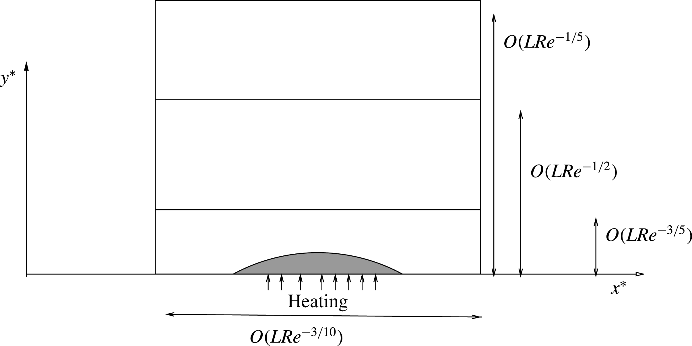
A schematic representation of the triple-deck region showing the heated hump.

We will be interested in transonic flows with the free-stream Mach number
 $M_{\infty }$
close to unity and consider
 $M_{\infty }^{2}=1+O(Re^{-1/5})$
as
 $Re\rightarrow \infty$
. A schematic of the triple-deck structure showing the different regions is depicted in figure 1. The motivation for these scalings arises from the argument first put forward by Messiter et al. (Reference Messiter, Feo and Melnik1971) for transonic flows and also discussed in Brilliant & Adamson (Reference Brilliant and Adamson1974) and Bodonyi & Kluwick (Reference Bodonyi and Kluwick1977). The reader is referred to these papers for more details and derivation of the triple-deck scalings.
In our problem we will assume that the effects of the heated hump are confined to the vicinity of the hump. Elsewhere the temperature is assumed constant and equal to unity. We assume that the hump has a length of
 $O(LRe^{-3/10})$
and height of
 $O(LRe^{-3/5})$
so that it is confined to the lower deck as in previous studies of localised heated elements in subsonic and supersonic flow by Koroteev & Lipatov (Reference Koroteev and Lipatov2012) for instance. This ensures that the temperature effects influence the flow nonlinearly in the interaction region.
The method of matched asymptotic expansions is now used to obtain the equations of the interaction problem with novel boundary conditions. We will consider each of the three regions of the triple deck in turn.
2.1 The main deck
In the main deck we have independent variables
 $$\begin{eqnarray}\displaystyle & \displaystyle x=1+Re^{-(3/10)}X,\quad y=Re^{-(1/2)}y_{2} & \displaystyle\end{eqnarray}$$
together with
 $$\begin{eqnarray}\displaystyle & \displaystyle M_{\infty }^{2}=1-Re^{-(1/5)}M_{1}, & \displaystyle\end{eqnarray}$$
where
 $M_{1}$
is an
 $O(1)$
parameter. The asymptotic expansions of the flow quantities are as follows:
 $$\begin{eqnarray}\displaystyle \left.\begin{array}{@{}l@{}}\displaystyle u=U_{B}(y_{2})+Re^{-(1/10)}u_{21}+\cdots \,,\quad v=Re^{-(3/10)}v_{21}+\cdots \,,\\[5.0pt] \displaystyle p=Re^{-(1/5)}p_{21}+\cdots \,,\quad \unicode[STIX]{x1D70C}=\unicode[STIX]{x1D70C}_{B}(y_{2})+Re^{-(1/10)}\unicode[STIX]{x1D70C}_{21}+\cdots \,,\\[5.0pt] \displaystyle h=h_{B}(y_{2})+Re^{-(1/10)}h_{21}+\cdots \quad T=T_{B}(y_{2})+Re^{-(1/10)}T_{21}+\cdots \,.\end{array}\right\} & & \displaystyle\end{eqnarray}$$
Here
 $U_{B}(y_{2})$
,
 $\unicode[STIX]{x1D70C}_{B}(y_{2}),h_{B}(y_{2})$
and
 $T_{B}(y_{2})$
are the non-dimensional Blasius velocity, density, enthalpy and temperature profiles respectively in the undisturbed boundary layer ahead of the higher-temperature zone. The basic flow properties are such that
 $$\begin{eqnarray}\displaystyle \left.\begin{array}{@{}l@{}}\displaystyle U_{B}(y_{2})\sim 1+O(\exp )\quad \text{as}~y_{2}\rightarrow \infty ,\\ \displaystyle \unicode[STIX]{x1D70C}_{B}(y_{2})\sim 1+O(\exp )\quad \text{as}~y_{2}\rightarrow \infty ,\\ \displaystyle T_{B}(y_{2})\sim 1+O(\exp )\quad \text{as}~y_{2}\rightarrow \infty ,\end{array}\right\} & & \displaystyle\end{eqnarray}$$
and
 $$\begin{eqnarray}\displaystyle & \displaystyle U_{B}(y_{2})\sim \unicode[STIX]{x1D706}y_{2}+O(y_{2}^{2}),\quad \unicode[STIX]{x1D70C}_{B}(y_{2})\sim 1+O(y_{2}),\quad T_{B}(y_{2})\sim 1+O(y_{2})\quad \text{as}~y_{2}\rightarrow 0, & \displaystyle \nonumber\\ \displaystyle & & \displaystyle\end{eqnarray}$$
with
 $\unicode[STIX]{x1D706}=(\text{d}U_{B}/\text{d}y_{2})|_{(y_{2}=0)}$
. The notation
 $O(\exp )$
denotes exponentially small terms in the limit
 $y_{2}\rightarrow \infty$
. We also have
 $$\begin{eqnarray}\displaystyle & \displaystyle (\unicode[STIX]{x1D6FE}-1)h_{B}=T_{B}=\frac{1}{\unicode[STIX]{x1D70C}_{B}}. & \displaystyle\end{eqnarray}$$
After substituting these expansions into (2.2)–(2.6) and solving the resultant equations we obtain
 $$\begin{eqnarray}\displaystyle \left.\begin{array}{@{}l@{}}\displaystyle u_{21}=A(X)\frac{\text{d}U_{B}}{\text{d}y_{2}},\quad v_{21}=-\frac{\text{d}A(X)}{\text{d}X}U_{B},\quad p_{21}=P(X),\\[12.0pt] \displaystyle T_{21}=A(X)\frac{\text{d}T_{B}}{\text{d}y_{2}}\quad \text{and}\quad \unicode[STIX]{x1D70C}_{21}=A(X)\frac{\text{d}\unicode[STIX]{x1D70C}_{B}}{\text{d}y_{2}}.\end{array}\right\} & & \displaystyle\end{eqnarray}$$
Here,
 $A(X)$
is an unknown displacement function.
2.2 The upper deck
For the upper deck, let
 $y=Re^{-1/5}y_{1}$
and we introduce the following asymptotic expansions:
 $$\begin{eqnarray}\displaystyle \left.\begin{array}{@{}l@{}}\displaystyle u=1+Re^{-(1/5)}u_{1}+Re^{-(2/5)}u_{2}+\cdots \,,\quad v=Re^{-(3/10)}v_{1}+Re^{-(1/2)}v_{2}+\cdots \,,\\[5.0pt] \displaystyle p=Re^{-(1/5)}p_{1}+Re^{-(2/5)}p_{2}+\cdots \,,\quad \unicode[STIX]{x1D70C}=1+Re^{-(1/5)}\unicode[STIX]{x1D70C}_{1}+Re^{-(2/5)}\unicode[STIX]{x1D70C}_{2}+\cdots \,,\\[5.0pt] \displaystyle h=h_{0}+Re^{-(1/5)}h_{1}+Re^{-(2/5)}h_{2}+\cdots \,.\end{array}\right\} & & \displaystyle\end{eqnarray}$$
After substituting into the governing equations it can be shown (see Perry Reference Perry2008, for instance) that the perturbed velocity potential
 $\unicode[STIX]{x1D719}_{1}$
defined by
 $$\begin{eqnarray}\displaystyle & \displaystyle u_{1}=\frac{\unicode[STIX]{x2202}\unicode[STIX]{x1D719}_{1}}{\unicode[STIX]{x2202}X},\quad v_{1}=\frac{\unicode[STIX]{x2202}\unicode[STIX]{x1D719}_{1}}{\unicode[STIX]{x2202}y_{1}} & \displaystyle\end{eqnarray}$$
satisfies the Kármán–Guderley equation:
 $$\begin{eqnarray}\displaystyle & \displaystyle [M_{1}-(\unicode[STIX]{x1D6FE}+1)u_{1}]{\displaystyle \frac{\unicode[STIX]{x2202}u_{1}}{\unicode[STIX]{x2202}X}}+{\displaystyle \frac{\unicode[STIX]{x2202}v_{1}}{\unicode[STIX]{x2202}y_{1}}}=0. & \displaystyle\end{eqnarray}$$
When the square bracketed term in (2.16) is positive the flow is subsonic and when it is negative the flow is supersonic. Also
 $$\begin{eqnarray}\displaystyle & \displaystyle p_{1}=\unicode[STIX]{x1D70C}_{1}=-u_{1}. & \displaystyle\end{eqnarray}$$
The conditions on
 $\unicode[STIX]{x1D719}_{1}$
are
 $$\begin{eqnarray}\displaystyle & \displaystyle \unicode[STIX]{x1D719}_{1}\rightarrow 0\quad \text{as}~X^{2}+y_{1}^{2}\rightarrow \infty & \displaystyle\end{eqnarray}$$
to match with the incident flow, and in addition
 $$\begin{eqnarray}\displaystyle & \displaystyle u_{1}(X,0)=-P(X),\quad v_{1}(X,0)=-{\displaystyle \frac{\text{d}A}{\text{d}X}}, & \displaystyle\end{eqnarray}$$
from matching with the main deck.
2.3 The lower deck
For the lower deck,
 $y=Re^{-3/5}y_{3}$
and the following asymptotic expansions hold:
 $$\begin{eqnarray}\displaystyle \left.\begin{array}{@{}l@{}}\displaystyle u=Re^{-(1/10)}u_{3}+\cdots \,,\quad v=Re^{-(2/5)}v_{3}+\cdots \,,\\ \displaystyle p=Re^{-(1/5)}p_{3}+\cdots \,,\quad \unicode[STIX]{x1D70C}=\unicode[STIX]{x1D70C}_{3}+\cdots \,,\\ \displaystyle \text{and}\quad T=T_{3}+\cdots \,.\end{array}\right\} & & \displaystyle\end{eqnarray}$$
Substituting these expansions into (2.2)–(2.6), we obtain
 $$\begin{eqnarray}\displaystyle & \displaystyle u_{3}{\displaystyle \frac{\unicode[STIX]{x2202}\unicode[STIX]{x1D70C}_{3}}{\unicode[STIX]{x2202}X}}+v_{3}{\displaystyle \frac{\unicode[STIX]{x2202}\unicode[STIX]{x1D70C}_{3}}{\unicode[STIX]{x2202}y_{3}}}+\unicode[STIX]{x1D70C}_{3}{\displaystyle \frac{\unicode[STIX]{x2202}u_{3}}{\unicode[STIX]{x2202}X}}+\unicode[STIX]{x1D70C}_{3}{\displaystyle \frac{\unicode[STIX]{x2202}v_{3}}{\unicode[STIX]{x2202}y_{3}}}=0, & \displaystyle\end{eqnarray}$$
 $$\begin{eqnarray}\displaystyle & \displaystyle \unicode[STIX]{x1D70C}_{3}\left(u_{3}{\displaystyle \frac{\unicode[STIX]{x2202}u_{3}}{\unicode[STIX]{x2202}X}}+v_{3}{\displaystyle \frac{\unicode[STIX]{x2202}u_{3}}{\unicode[STIX]{x2202}y_{3}}}\right)=-{\displaystyle \frac{\unicode[STIX]{x2202}p_{3}}{\unicode[STIX]{x2202}X}}+{\displaystyle \frac{\unicode[STIX]{x2202}}{\unicode[STIX]{x2202}y_{3}}}\left(\unicode[STIX]{x1D707}{\displaystyle \frac{\unicode[STIX]{x2202}u_{3}}{\unicode[STIX]{x2202}y_{3}}}\right), & \displaystyle\end{eqnarray}$$
 $$\begin{eqnarray}\displaystyle & \displaystyle {\displaystyle \frac{\unicode[STIX]{x2202}p_{3}}{\unicode[STIX]{x2202}y_{3}}}=0, & \displaystyle\end{eqnarray}$$
 $$\begin{eqnarray}\displaystyle & \displaystyle \unicode[STIX]{x1D70C}_{3}\left(u_{3}{\displaystyle \frac{\unicode[STIX]{x2202}T_{3}}{\unicode[STIX]{x2202}X}}+v_{3}{\displaystyle \frac{\unicode[STIX]{x2202}T_{3}}{\unicode[STIX]{x2202}y_{3}}}\right)={\displaystyle \frac{\unicode[STIX]{x2202}}{\unicode[STIX]{x2202}y}}\left({\displaystyle \frac{\unicode[STIX]{x1D707}}{Pr}}{\displaystyle \frac{\unicode[STIX]{x2202}T_{3}}{\unicode[STIX]{x2202}y_{3}}}\right), & \displaystyle\end{eqnarray}$$
 $$\begin{eqnarray}\displaystyle & \displaystyle \unicode[STIX]{x1D70C}_{3}T_{3}=1. & \displaystyle\end{eqnarray}$$
To match with the oncoming basic boundary layer flow far upstream we require that
 $$\begin{eqnarray}\displaystyle & \displaystyle u_{3}\rightarrow \unicode[STIX]{x1D706}y_{3},\quad T_{3}\rightarrow 1,\quad p_{3}\rightarrow 0,\quad A(X)\rightarrow 0,\quad \text{as}~X\rightarrow -\infty . & \displaystyle\end{eqnarray}$$
The boundary conditions on the hump
 $y_{3}=F(X)$
are
 $$\begin{eqnarray}\displaystyle & \displaystyle u_{3}=v_{3}=0\quad \text{and}\quad T_{3}=T_{w}(X), & \displaystyle\end{eqnarray}$$
where
 $T_{w}(X)$
is some prescribed wall temperature function. Finally
 $$\begin{eqnarray}\displaystyle & \displaystyle p_{3}=P(X),\quad u_{3}\rightarrow \unicode[STIX]{x1D706}(A(X)+y_{3})\quad \text{and}\quad T_{3}\rightarrow 1\quad \text{as}~y_{3}\rightarrow \infty & \displaystyle\end{eqnarray}$$
in order to match with the main deck.
2.4 Viscous–inviscid interaction problem
The Kármán–Guderley equation for the upper deck (2.16), needs to be solved simultaneously with the boundary layer equations (2.21)–(2.25) and boundary conditions. The equations can be reduced to a more standard form via a Prandtl transformation and the constant
 $\unicode[STIX]{x1D706}$
can also be scaled out of the problem by using the substitutions
 $$\begin{eqnarray}\displaystyle \left.\begin{array}{@{}l@{}}\displaystyle X=\unicode[STIX]{x1D706}^{-(7/5)}X_{b},\quad y_{3}=\unicode[STIX]{x1D706}^{-(4/5)}(y_{3b}+F_{b}),\quad y_{1}=\unicode[STIX]{x1D706}^{-(8/5)}y_{1b},\\[5.0pt] \displaystyle u_{3}=\unicode[STIX]{x1D706}^{1/5}u_{3b},\quad v_{3}=\unicode[STIX]{x1D706}^{4/5}\left[v_{3b}+u_{3b}{\displaystyle \frac{\unicode[STIX]{x2202}F_{b}}{\unicode[STIX]{x2202}X_{b}}}\right],\quad p_{3}=\unicode[STIX]{x1D706}^{2/5}p_{3b},\\[12.0pt] \displaystyle F=\unicode[STIX]{x1D706}^{-(4/5)}F_{b},\quad A=\unicode[STIX]{x1D706}^{-(4/5)}{\mathcal{A}},\quad M_{1}=\unicode[STIX]{x1D706}^{2/5}\unicode[STIX]{x1D712},\\[5.0pt] \displaystyle \unicode[STIX]{x1D70C}_{3}=\unicode[STIX]{x1D70C}_{b},\quad T_{3}=T_{b},\\[5.0pt] \displaystyle u_{1}=\unicode[STIX]{x1D706}^{2/5}u_{1b}\quad \text{and}\quad v_{1}=\unicode[STIX]{x1D706}^{3/5}v_{1b}.\end{array}\right\} & & \displaystyle\end{eqnarray}$$
A further, more convenient, form of the equations suitable for computations is obtained by using the Howarth–Dorodnitsyn transformation in which we transform from
 $(X_{b},y_{3b})\rightarrow (x_{b},y_{b})$
variables given by
 $$\begin{eqnarray}\displaystyle & \displaystyle y_{b}=\int _{0}^{y_{3b}}\unicode[STIX]{x1D70C}_{3}(X_{b},\unicode[STIX]{x1D702})\,\text{d}\unicode[STIX]{x1D702},\quad x_{b}=X_{b} & \displaystyle\end{eqnarray}$$
and
 $$\begin{eqnarray}\displaystyle & \displaystyle u_{b}=u_{3b},\quad v_{3b}={\displaystyle \frac{1}{\unicode[STIX]{x1D70C}_{3}}}\left[v_{b}-u_{b}{\displaystyle \frac{\unicode[STIX]{x2202}y_{b}}{\unicode[STIX]{x2202}x_{b}}}\right]. & \displaystyle\end{eqnarray}$$
In addition, we assume that the viscosity coefficient depends linearly on the temperature and is given by Chapman’s law
 $\unicode[STIX]{x1D70C}_{3}\unicode[STIX]{x1D707}=1$
. As a result we obtain the final set of equations
 $$\begin{eqnarray}\displaystyle & \displaystyle {\displaystyle \frac{\unicode[STIX]{x2202}u_{b}}{\unicode[STIX]{x2202}x_{b}}}+{\displaystyle \frac{\unicode[STIX]{x2202}v_{b}}{\unicode[STIX]{x2202}y_{b}}}=0, & \displaystyle\end{eqnarray}$$
 $$\begin{eqnarray}\displaystyle & \displaystyle u_{b}{\displaystyle \frac{\unicode[STIX]{x2202}u_{b}}{\unicode[STIX]{x2202}x_{b}}}+v_{b}{\displaystyle \frac{\unicode[STIX]{x2202}u_{b}}{\unicode[STIX]{x2202}y_{b}}}+T_{b}{\displaystyle \frac{\unicode[STIX]{x2202}p_{b}}{\unicode[STIX]{x2202}x_{b}}}={\displaystyle \frac{\unicode[STIX]{x2202}^{2}u_{b}}{\unicode[STIX]{x2202}y_{b}^{2}}}, & \displaystyle\end{eqnarray}$$
 $$\begin{eqnarray}\displaystyle & \displaystyle u_{b}{\displaystyle \frac{\unicode[STIX]{x2202}T_{b}}{\unicode[STIX]{x2202}x_{b}}}+v_{b}{\displaystyle \frac{\unicode[STIX]{x2202}T_{b}}{\unicode[STIX]{x2202}y_{b}}}=\frac{1}{Pr}{\displaystyle \frac{\unicode[STIX]{x2202}^{2}T_{b}}{\unicode[STIX]{x2202}y_{b}^{2}}}. & \displaystyle\end{eqnarray}$$
The no-slip conditions are now applied on
 $y_{b}=0$
with
 $$\begin{eqnarray}\displaystyle & \displaystyle u_{b}(x_{b},0)=v_{b}(x_{b},0)=0 & \displaystyle\end{eqnarray}$$
and the prescribed wall temperature
 $$\begin{eqnarray}\displaystyle & \displaystyle T_{b}(x_{b},0)=T_{w}(x_{b}). & \displaystyle\end{eqnarray}$$
The boundary conditions as
 $y_{b}\rightarrow \infty$
are given by
 $$\begin{eqnarray}\displaystyle & \displaystyle u_{b}\rightarrow y_{b}+{\mathcal{A}}(x_{b})+H(x_{b}), & \displaystyle\end{eqnarray}$$
 $$\begin{eqnarray}\displaystyle & \displaystyle T_{b}(x_{b},y_{b})\rightarrow 1. & \displaystyle\end{eqnarray}$$
Also,
 $$\begin{eqnarray}\displaystyle & \displaystyle {\mathcal{A}}(x_{b})\rightarrow 0\quad \text{as}~x_{b}\rightarrow -\infty . & \displaystyle\end{eqnarray}$$
In the above the physical hump shape
 $F(x_{b})$
is related to the transformed hump shape
 $H(x_{b})$
via
 $$\begin{eqnarray}\displaystyle & \displaystyle H(x_{b})=\int _{0}^{F(x_{b})}\unicode[STIX]{x1D70C}_{3}(x_{b},\unicode[STIX]{x1D702})\,\text{d}\unicode[STIX]{x1D702}. & \displaystyle\end{eqnarray}$$
The upper deck equations and boundary conditions are
 $$\begin{eqnarray}\displaystyle & \displaystyle [\unicode[STIX]{x1D712}-(\unicode[STIX]{x1D6FE}+1)u_{1b}]{\displaystyle \frac{\unicode[STIX]{x2202}u_{1b}}{\unicode[STIX]{x2202}x_{b}}}+{\displaystyle \frac{\unicode[STIX]{x2202}v_{1b}}{\unicode[STIX]{x2202}y_{1b}}}=0, & \displaystyle\end{eqnarray}$$
 $$\begin{eqnarray}\displaystyle & \displaystyle {\displaystyle \frac{\unicode[STIX]{x2202}u_{1b}}{\unicode[STIX]{x2202}y_{1b}}}-{\displaystyle \frac{\unicode[STIX]{x2202}v_{1b}}{\unicode[STIX]{x2202}x_{b}}}=0, & \displaystyle\end{eqnarray}$$
with
 $$\begin{eqnarray}\displaystyle & \displaystyle p_{b}(x_{b})=-u_{1b}(x_{b},0)\quad \text{and}\quad v_{1b}(x_{b},0)=-{\displaystyle \frac{\text{d}{\mathcal{K}}}{\text{d}x_{b}}}, & \displaystyle\end{eqnarray}$$
where
 $$\begin{eqnarray}\displaystyle & \displaystyle {\mathcal{K}}(x_{b})={\mathcal{A}}(x_{b})+\int _{0}^{\infty }(1-T_{b}(x_{b},\unicode[STIX]{x1D702}))\,\text{d}\unicode[STIX]{x1D702}. & \displaystyle\end{eqnarray}$$
The latter expression arises as in previous related studies with localised heating: see Lipatov (Reference Lipatov2006) and Koroteev & Lipatov (Reference Koroteev and Lipatov2012).
3 Numerical solution of the coupled viscous–inviscid interaction problem
In order to solve the above equations, finite differences are used for discretising the derivatives in the
 $x_{b}$
-direction and Chebyshev collocation is used for derivatives in the
 $y_{b}$
- and
 $y_{1b}$
-directions. The method used to solve the Kármán–Guderley equation is very similar to that presented in Pereira & Gajjar (Reference Pereira and Gajjar2010, Reference Pereira, Gajjar and Assi2011) for transonic flow past aerofoils, and takes account of the mixed-type differencing, as described in Murman & Cole (Reference Murman and Cole1971) and Cole & Cook (Reference Cole and Cook1986) for subsonic, supersonic or shock points. The equations (2.32)–(2.44) governing the viscous–inviscid interaction are nonlinear. The nonlinearity is exhibited even in the upper deck equations, in contrast to subsonic or supersonic flows where the upper deck equations reduce to linear equations. In order to deal with this we use a Newton–Raphson linearisation and then solve the resulting system for the correction terms.
For the solution of the triple-deck equations in the lower deck, we used a similar approach to that described in Logue, Gajjar & Ruban (Reference Logue, Gajjar and Ruban2014) for solving the steady equations in that paper. For attached flows backward differences are used to discretise the convective terms in the lower deck and forward differences for separated flows. A similar approach is used to handle the
 $u_{b}\unicode[STIX]{x2202}T_{b}/\unicode[STIX]{x2202}x_{b}$
term as well.
As a result, if we denote the unknowns variables at
 $x=x_{i}$
by
 $$\begin{eqnarray}\displaystyle & \displaystyle \text{}\underline{{\mathcal{L}}}_{i}=\left(\text{}\underline{\unicode[STIX]{x1D6F7}}_{i},\text{}\underline{{\mathcal{U}}}_{i},\text{}\underline{U}_{i},\text{}\underline{T}_{i},P_{i},\text{A}_{i},K_{i}\right)^{\text{T}}, & \displaystyle\end{eqnarray}$$
where for example
 $$\begin{eqnarray}\displaystyle & \displaystyle \unicode[STIX]{x1D6F7}_{i}=(\unicode[STIX]{x1D719}_{i,0},\unicode[STIX]{x1D719}_{i,1},\ldots ,\unicode[STIX]{x1D719}_{i,S})^{\text{T}} & \displaystyle\end{eqnarray}$$
is the vector of unknowns perturbation potentials at
 $x=x_{i}$
, and with a similar notation for the streamwise velocity
 ${\mathcal{U}}_{i}$
unknowns in the upper deck,
 $U_{i}$
the
 $u$
-velocity in the lower deck,
 $T_{i}$
the temperature unknowns at
 $x=x_{i}$
, then the equation system can be written as
 $$\begin{eqnarray}\displaystyle & \displaystyle A_{i}\text{}\underline{{\mathcal{L}}}_{i-2}+B_{i}\text{}\underline{{\mathcal{L}}}_{i-1}+C_{i}\text{}\underline{{\mathcal{L}}}_{i}+F_{i}\text{}\underline{{\mathcal{L}}}_{i+1}+E_{i}\text{}\underline{{\mathcal{L}}}_{i+2}=\text{}\underline{Q}_{i}, & \displaystyle\end{eqnarray}$$
where
 $A_{i},B_{i},C_{i},F_{i}$
and
 $E_{i}$
are of size
 $(2S+2N+7)\times (2S+2N+7)$
.
This discrete system is applied to
 $3\leqslant i\leqslant (M-2)$
, while for
 $i<3$
we impose values that are given by undisturbed boundary layer profiles, i.e.
 ${\mathcal{U}}=\unicode[STIX]{x1D6F7}=0$
,
 $U=y_{b}$
,
 $T=1$
,
 ${\mathcal{K}}=0$
and
 $P=0$
. For
 $i>(M-2)$
one-sided differences are used. A detailed description of the full discretised system can be found in Aljohani (Reference Aljohani2016).
4 Results
The results in general depend on three key parameters which are the Kármán–Guderley parameter
 $\unicode[STIX]{x1D712}$
, the height of the element
 $h$
and the amplitude of the temperature perturbations
 $\unicode[STIX]{x0394}T$
. In particular, the results are qualitatively different for different signs of
 $\unicode[STIX]{x1D712}$
. In the results shown below (unless otherwise stated) we use the wall heating function given by
 $$\begin{eqnarray}\displaystyle \displaystyle T_{w}(x_{b})=\left\{\begin{array}{@{}ll@{}}\displaystyle 1+\unicode[STIX]{x0394}T & |x_{b}|\leqslant {\displaystyle \frac{a}{2}},\\[12.0pt] \displaystyle 1 & |x_{b}|>{\displaystyle \frac{a}{2}},\end{array}\right. & & \displaystyle\end{eqnarray}$$
where
 $\unicode[STIX]{x0394}T$
is the amplitude of perturbations of the temperature and
 $a$
is the extent of the heating region. We have also taken the Prandtl number to be equal to unity.
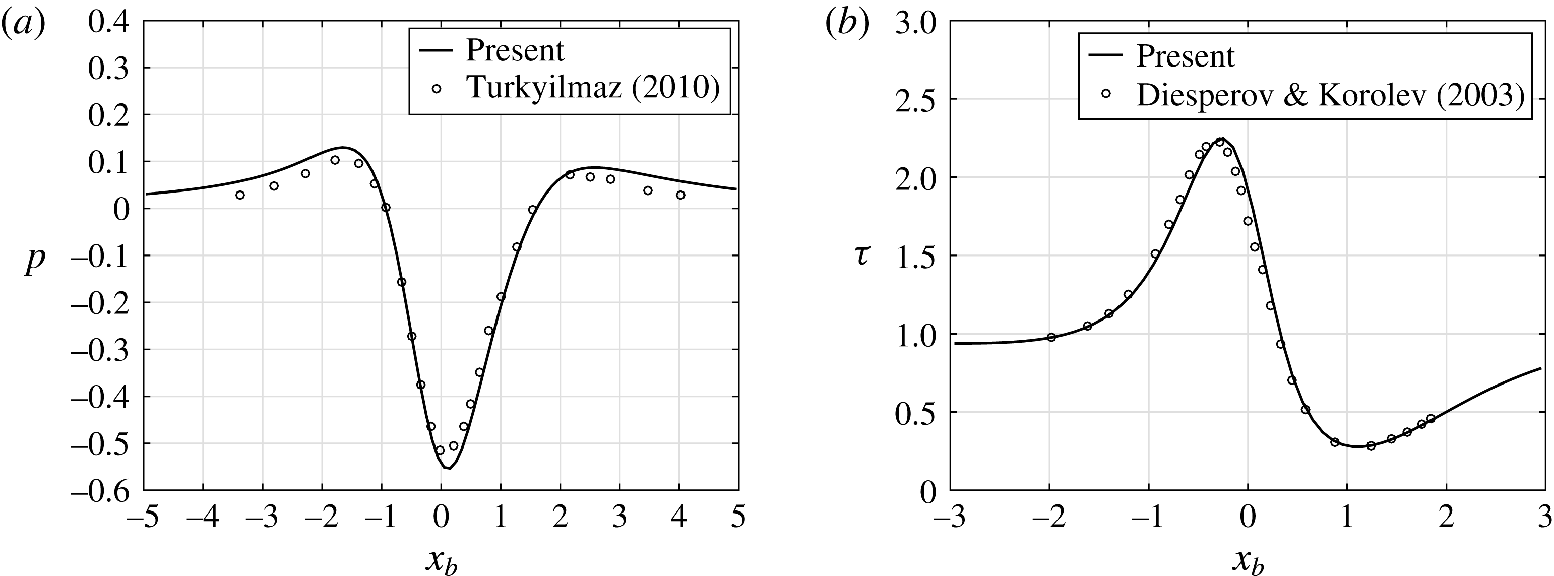
Comparisons with previous work. (a) Pressure distribution
 $p$
for
 $\unicode[STIX]{x1D712}=2,h=1.5$
for the shape
 $H(x)=h\text{e}^{-x^{2}}$
. The symbols denote the results of Turkyilmaz (Reference Turkyilmaz2010). (b) Wall shear distribution
 $\unicode[STIX]{x1D70F}$
for
 $\unicode[STIX]{x1D712}=3,h=3$
and with
 $H(x)=h/(1+x^{2})$
. The symbols are from the work of Diesperov & Korolev (Reference Diesperov and Korolev2003).

For the unheated hump with
 $\unicode[STIX]{x0394}T=0$
, we can compare with previous work. Turkyilmaz (Reference Turkyilmaz2010) studied a problem of transonic flow past over general wall irregularities such as a hump on a rigid body surface. He chose the hump shape as
 $$\begin{eqnarray}\displaystyle & \displaystyle H(x)=h\text{e}^{-x^{2}}. & \displaystyle\end{eqnarray}$$
Diesperov & Korolev (Reference Diesperov and Korolev2003) investigated the transonic flow past roughness situated in the lower viscous sublayer. They selected the hump shape to be
 $$\begin{eqnarray}\displaystyle & \displaystyle H(x)={\displaystyle \frac{h}{1+x^{2}}}. & \displaystyle\end{eqnarray}$$
Figure 2(a) shows a comparison between the pressure distribution exhibited in Turkyilmaz (Reference Turkyilmaz2010) and our results, and in figure 2(b) we present a comparison of the wall shear distribution
 $\unicode[STIX]{x1D70F}=\unicode[STIX]{x2202}u_{b}/\unicode[STIX]{x2202}y_{b}(x_{b},0)$
from the work of Diesperov & Korolev (Reference Diesperov and Korolev2003) and our results. Good agreement between the results can be deduced in both figures 2(a) and 2(b), although it is noted that for these cases the flow is attached. In figure 3 we present a comparison of the function
 $-{\mathcal{A}}(x_{b})$
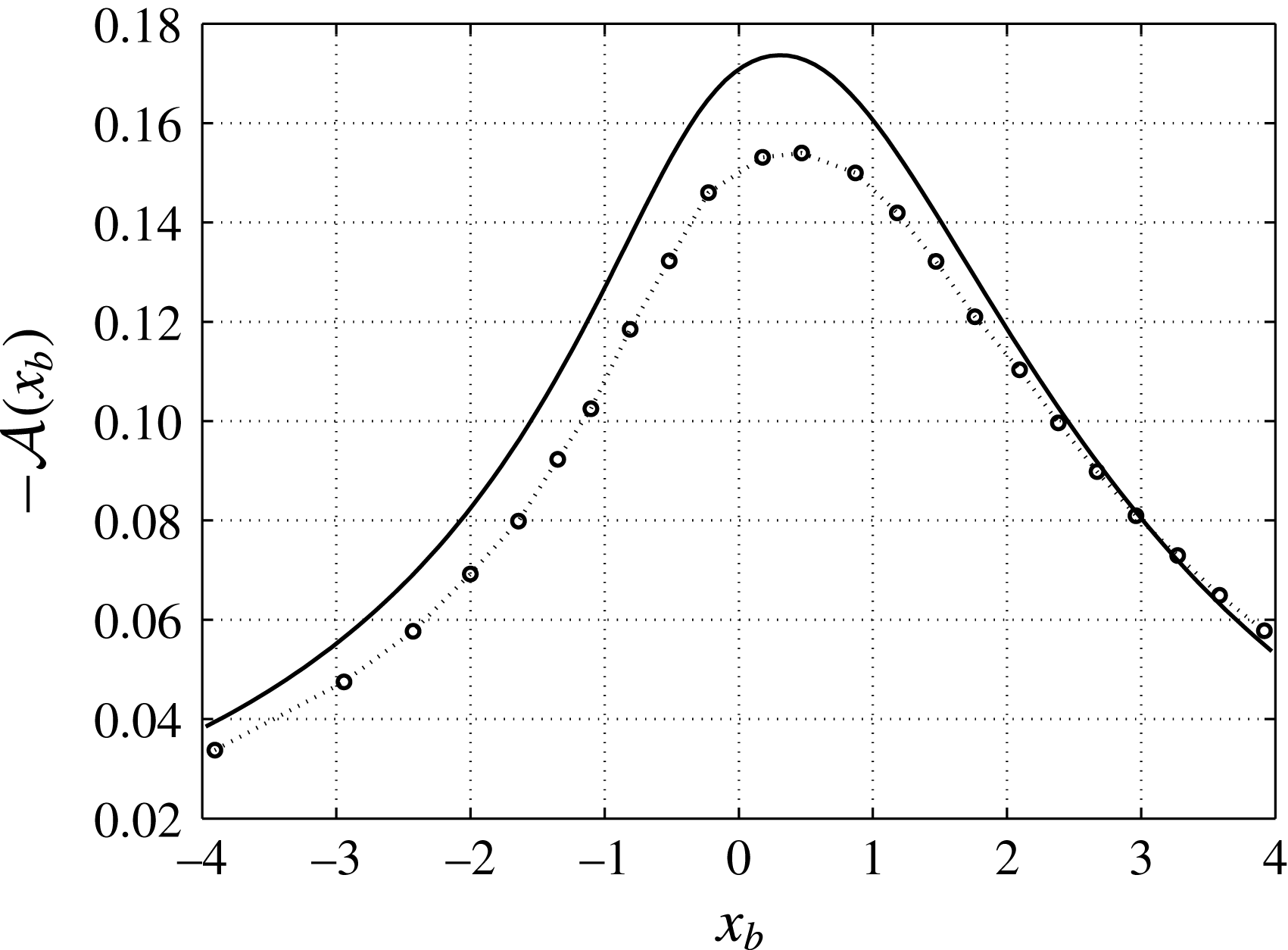
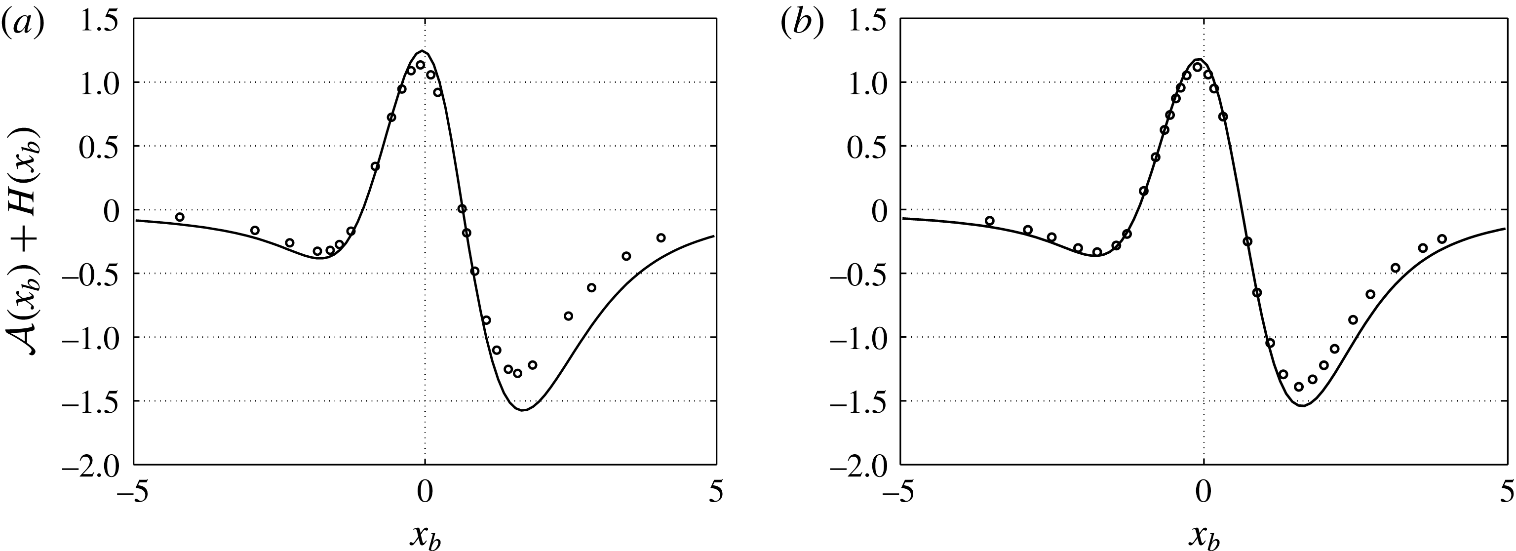
, the displacement function, with the results of Diesperov & Korolev (Reference Diesperov and Korolev2003). There are discrepancies in the results which may be due to the different numerical techniques used. Similarly a comparison of the function
 ${\mathcal{A}}(x_{b})+H(x_{b})$
with the results in Turkyilmaz (Reference Turkyilmaz2010) is presented in figure 4 for two different values of
 $\unicode[STIX]{x1D712}$
. Our results agree well on most of the hump except towards the rear of the hump where we have a lower minimum value as compared to the results shown in Turkyilmaz (Reference Turkyilmaz2010). With the numerical method used by Turkyilmaz (Reference Turkyilmaz2010) the maximum height of a hump that he could compute with for separated flow was
 $h=3.6$
with
 $\unicode[STIX]{x1D712}=2$
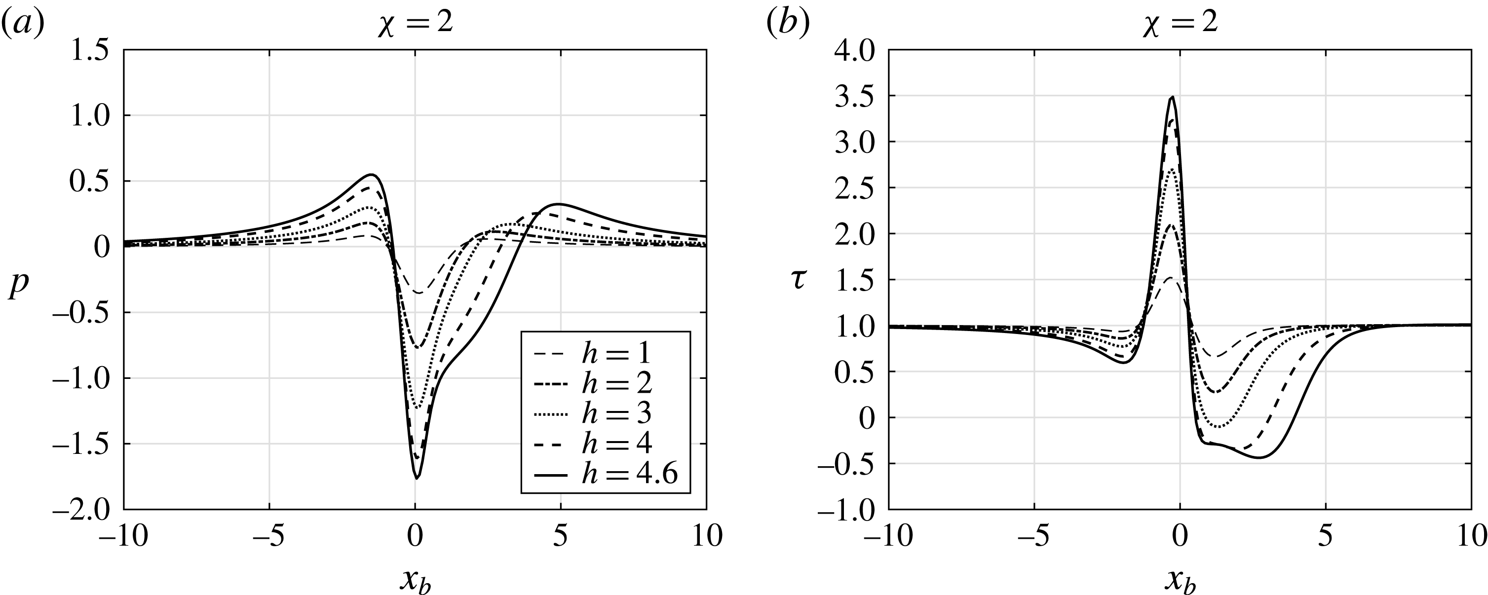
. This may account for the differences as Turkyilmaz (Reference Turkyilmaz2010) was unable to cope with mixed-type flow occurring in the upper deck. Using our numerical method we were able to compute larger separated regions up to
 $h=4.6$
as shown in figures 5(a) and 5(b).
Comparison of
 $-{\mathcal{A}}(x_{b})$
with the results of Diesperov & Korolev (Reference Diesperov and Korolev2003) (shown by symbols) and the present results (shown by the solid line) for the hump shape
 $H(x)=h/(1+x^{2})$
with
 $h=0.35$
and
 $\unicode[STIX]{x1D712}=0.3$
.

Comparisons of the function
 ${\mathcal{A}}(x_{b})+H(x_{b})$
with Turkyilmaz (Reference Turkyilmaz2010) (shown by the symbols) with the present results (shown by the solid line) for the hump shape
 $H(x)=h\text{e}^{-x^{2}}$
. (a)
 $h=3.5,\unicode[STIX]{x1D712}=2$
and (b)
 $h=3.8,\unicode[STIX]{x1D712}=3$
.

Distributions of (a) pressure and (b) wall shear for different values of
 $h=1,2,3,4$
and
 $4.6$
for the shape
 $H(x)=h\text{e}^{-x^{2}}$
.

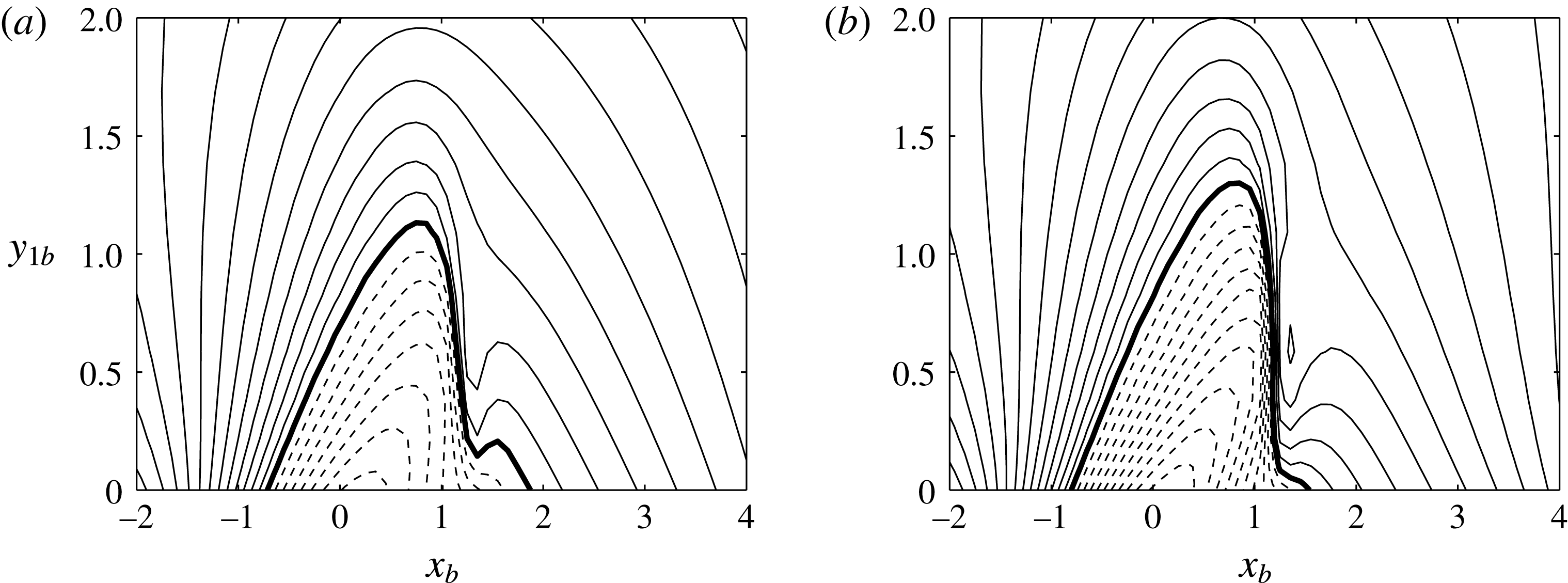
In the work of Diesperov & Korolev (Reference Diesperov and Korolev2003) embedded supersonic zones in a predominantly subsonic flow were observed for large hump heights. A similar observation is made here as well but for the heated hump. Taking the wall temperature profile to be given as in (4.1) with
 $a=10$
and
 $h=6$
, we have plotted contours of the function
 $$\begin{eqnarray}\displaystyle & \displaystyle R(x_{b},y_{1b})=\unicode[STIX]{x1D712}-(\unicode[STIX]{x1D6FE}+1)u_{1b}(x_{b},y_{1b}) & \displaystyle\end{eqnarray}$$
for
 $\unicode[STIX]{x1D712}=2$
for the heated case with
 $\unicode[STIX]{x0394}T=1$
in figure 6(a), and the unheated case with
 $\unicode[STIX]{x0394}T=0$
in figure 6(b). Subsonic zones are present when
 $R>0$
and supersonic zones when
 $R<0$
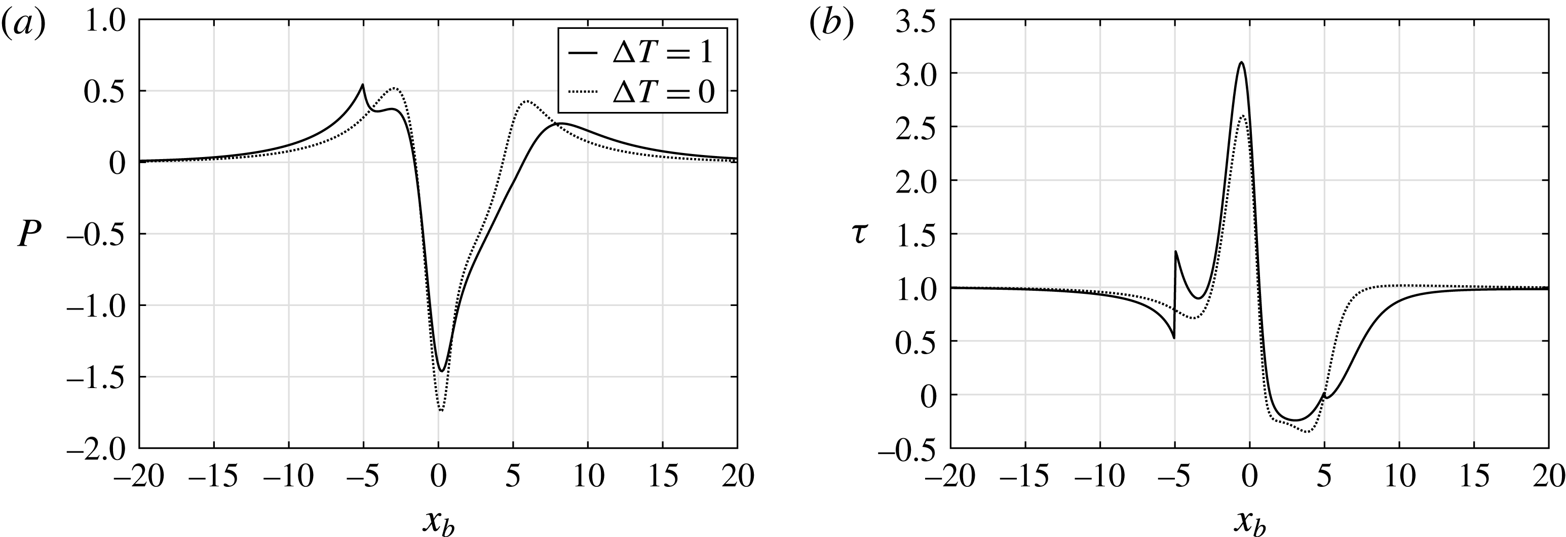
. A two-hump supersonic zone can be recognised from figure 6 where shock waves are formed. This is similar to that found by Diesperov & Korolev (Reference Diesperov and Korolev2003). The pressure distribution starts rising in this area as shown in figure 7(a). In figure 7(b) the wall shear distribution exhibits a rapid drop leading to separation starting just after the top of the hump is reached. The sharp rise in the wall shear at
 $x_{b}=-5$
and the smaller drop at
 $x_{b}=5$
coincide with the start and end of the wall heating region. Heating is seen to be slightly beneficial as far as reducing separation is concerned.
Contours of
 $R$
for
 $\unicode[STIX]{x1D712}=2$
and
 $h=6$
. Contour intervals are in steps of 0.2 and dashed lines denote negative contours; the solid line denotes the zero contour. (a)
 $\unicode[STIX]{x0394}T=1$
, (b)
 $\unicode[STIX]{x0394}T=0$
. The hump shape is
 $H(x)=h/(1+x^{2})$
.

Distributions of (a) pressure and (b) wall shear with
 $\unicode[STIX]{x1D712}=2$
and
 $h=6$
.

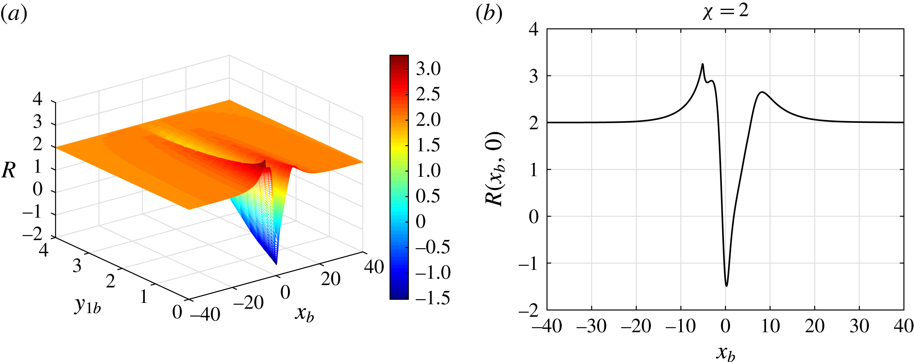
In figure 8(a) we have displayed a plot of the function
 $R(x_{b},y_{1b})$
and in figure 8(b) the curve
 $R(x_{b},0)$
is shown. Supersonic zones are determined when
 $R<0$
and it can be seen that the supersonic zones are located near the top of the hump and are strongest near the wall.
(a)
 $R(x_{b},y_{1b})$
and (b)
 $R(x_{b},0)$
where supersonic zones are determined when
 $R<0$
where
 $\unicode[STIX]{x0394}T=1$
and
 $h=6$
.

The effects of varying
 $h$
and
 $\unicode[STIX]{x0394}T$
are studied next for negative and positive values of the Kármán–Guderley parameter
 $\unicode[STIX]{x1D712}$
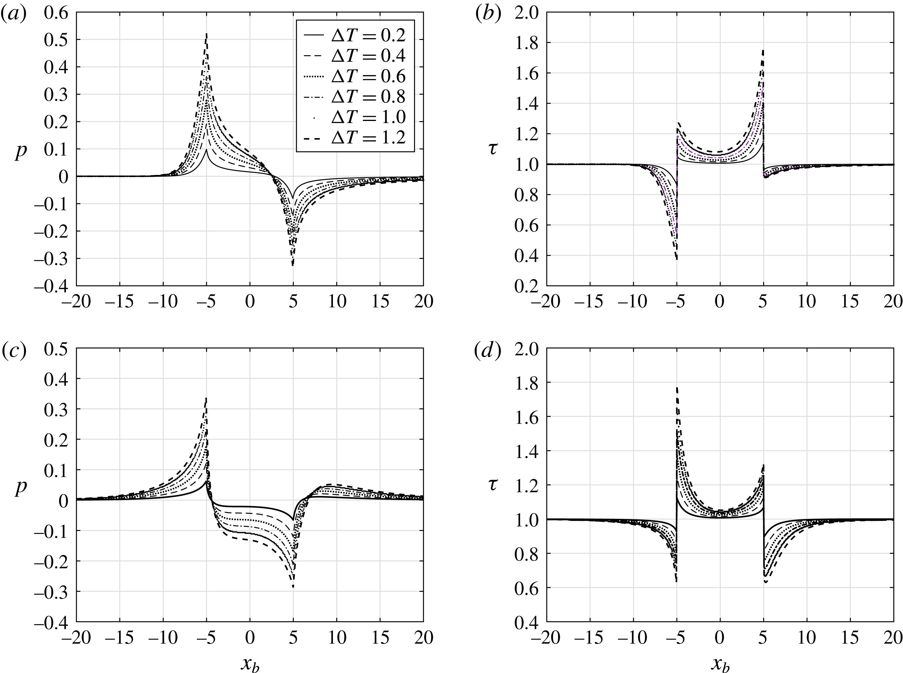
. In figure 9(a–d) we show the flat-plate case
 $h=0$
with varying
 $\unicode[STIX]{x0394}T$
. The pressure rises ahead of the heating element and then drops monotonically until the end of the element is reached, after which the pressure rises again. The skin friction on the other hand is falling ahead of the element, but the effect of the heating generates a stronger attached flow once the flow enters the heated region. The rise and drop in the pressure, and shear especially is quite abrupt at the start and end of the heated region. Comparing the
 $\unicode[STIX]{x1D712}=-2$
results in figure 9(a,b) and the
 $\unicode[STIX]{x1D712}=2$
results in figure 9(c,d) there are clear differences for supersonic
 $(\unicode[STIX]{x1D712}=-2)$
and subsonic flows
 $(\unicode[STIX]{x1D712}=2)$
. In the former the drop in the wall shear is largest ahead of the heated element, whilst in the latter the drop is largest behind the element. This suggests that in supersonic flows, heated elements even though they help in producing more attached flow over the elements, could also provoke a free interaction ahead of the element, especially with strong heating (
 $\unicode[STIX]{x0394}T\gg 1$
).
Results for the flat-plate case with
 $h=0$
and
 $a=10$
for different
 $\unicode[STIX]{x0394}T$
. (a) Pressure
 $p$
with
 $\unicode[STIX]{x1D712}=-2$
, (b) wall shear
 $\unicode[STIX]{x1D70F}$
with
 $\unicode[STIX]{x1D712}=-2$
, (c) pressure
 $p$
with
 $\unicode[STIX]{x1D712}=2$
and (d) wall shear
 $\unicode[STIX]{x1D70F}$
with
 $\unicode[STIX]{x1D712}=2$
.

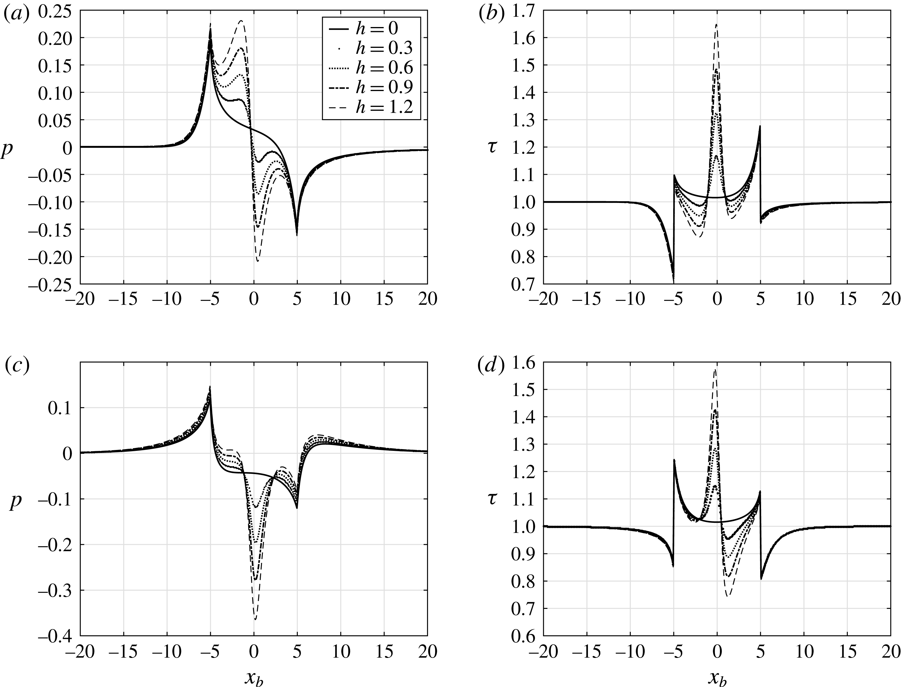
Results for the hump-shaped element with
 $H(x)=h/(1+x^{2})$
shown in figure 10(a–d) indicate that there are additional peaks and troughs in the pressure and wall shear over the hump. The pressure and wall shear distributions have a very similar behaviour to the supersonic and subsonic flow over heated humps results shown in Aljohani (Reference Aljohani2016) and Aljohani & Gajjar (Reference Aljohani and Gajjar2017a
,Reference Aljohani and Gajjar
b
). In the supersonic flow the pressure peaks just before the top of the hump and drops substantially, recovering again once the hump is negotiated. In the subsonic flow the pressure drops in the vicinity of the top of the hump reaching a minimum at the peak before recovering. The wall shear distributions in figure 10(b,d) also show that in subsonic flow there is a much larger drop after the top of the hump is negotiated. In comparison with the flat-plate case, the heated hump shows a much stronger attached flow near the top of the hump. The maximum pressure and shear points move from the boundaries of the element to the neighbourhood of the centre of the element with increasing
 $h$
.
Results with
 $\unicode[STIX]{x0394}T=0.4$
and
 $a=10$
for different values of
 $h$
for the wall shape
 $H(x)=h/(1+x^{2})$
. (a) Pressure
 $p$
with
 $\unicode[STIX]{x1D712}=-2$
, (b) wall shear
 $\unicode[STIX]{x1D70F}$
with
 $\unicode[STIX]{x1D712}=-2$
, (c) pressure
 $p$
with
 $\unicode[STIX]{x1D712}=2$
and (d) wall shear
 $\unicode[STIX]{x1D70F}$
with
 $\unicode[STIX]{x1D712}=2$
.

The relation between flow separation and the Kármán–Guderley parameter
 $\unicode[STIX]{x1D712}$
is investigated next. The effects of varying
 $\unicode[STIX]{x1D712}$
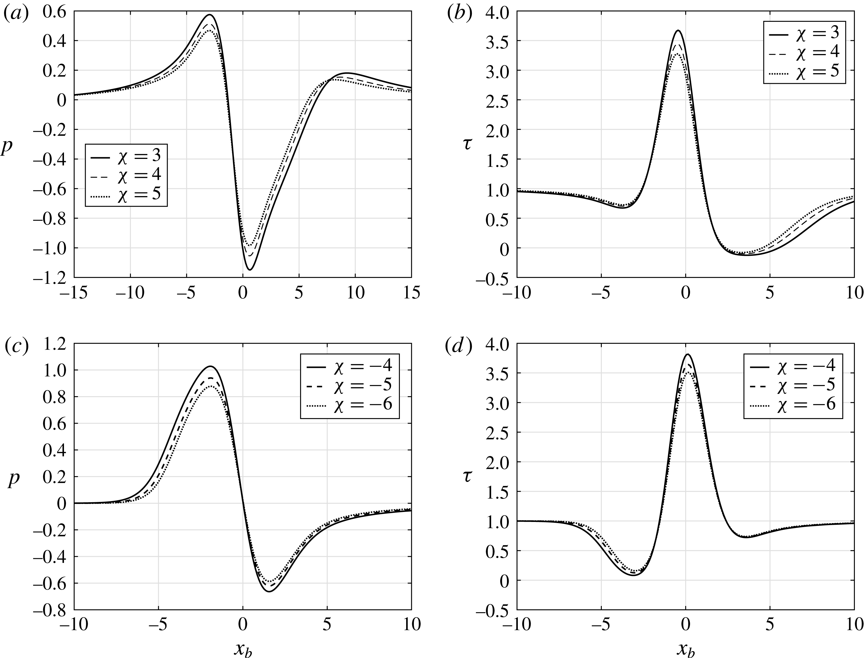
on the results are presented in figure 11(a–d) where
 $h=4$
and
 $\unicode[STIX]{x0394}T=4$
for different values of
 $\unicode[STIX]{x1D712}$
. For the results shown in figure 11 the wall temperature function is given by
 $T_{w}(x_{b})=1+\unicode[STIX]{x0394}T\text{e}^{-0.25x_{b}^{2}}$
. It can be inferred that increasing the Kármán–Guderley parameter
 $|\unicode[STIX]{x1D712}|$
leads to an increase in the values of the critical
 $h$
and
 $\unicode[STIX]{x0394}T$
for determining the start of flow separation. The flow has a greater tendency towards separation in the transonic regime with
 $|\unicode[STIX]{x1D712}|$
decreasing towards unity.
Distributions of the pressure
 $p$
and wall shear
 $\unicode[STIX]{x1D70F}$
with
 $h=4$
and
 $\unicode[STIX]{x0394}T=4$
. The wall heating profile is
 $T_{w}(x)=1+\unicode[STIX]{x0394}T\text{e}^{-0.25x^{2}}$
and the hump shape is
 $H(x)=h\text{e}^{-0.25x^{2}}$
.

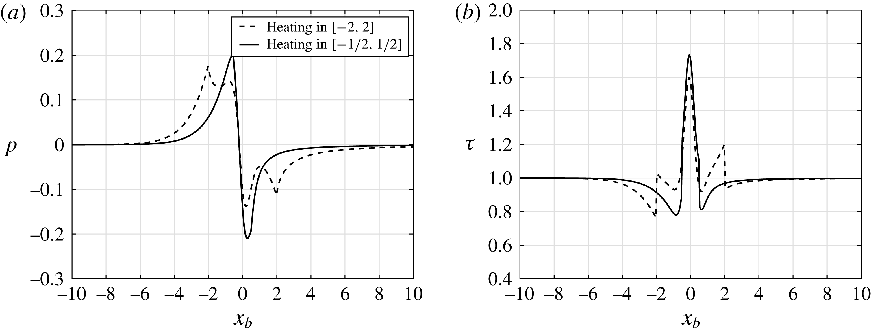
Figure 12(a,b) indicates that the effect of changing the extent of the heated region on the pressure and wall shear with the hump shape
 $H(x)=h\text{e}^{-5x^{2}}$
and the temperature profile as given by (4.1) for
 $\unicode[STIX]{x1D712}=-2$
. The two curves in figure 12(a,b) are with
 $a=4$
and
 $a=1$
. Reducing the extent of the heated region
 $(a=1)$
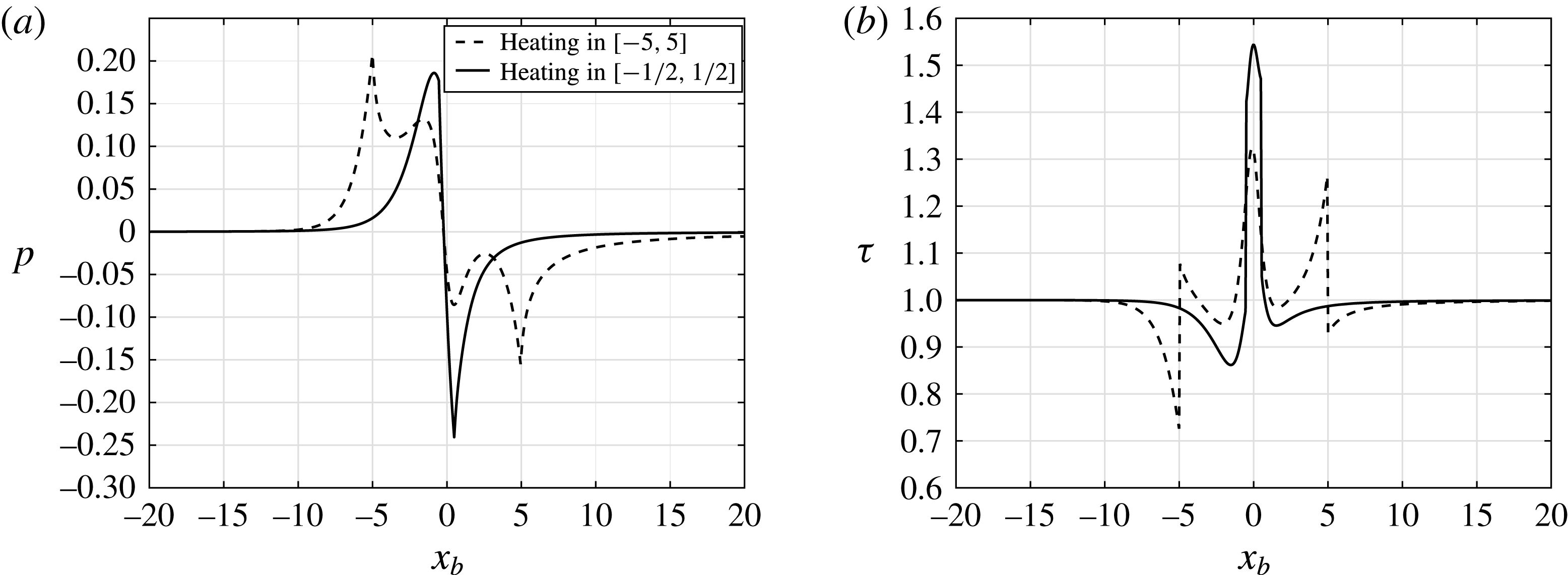
generates a smoother change to attached flow over the heated element. The abrupt almost discontinuous change in the wall shear is strongly related to where the heated region starts and ends. This behaviour has also been previously observed in the study by Koroteev & Lipatov (Reference Koroteev and Lipatov2009) for supersonic flow over heated flat-plate elements and Aljohani & Gajjar (Reference Aljohani and Gajjar2017a
) for subsonic flow over humps. The effect of different heated regions with the same wall temperature profile but with a slightly different hump shape
 $H(x)=h/(1+x^{2})$
is shown in figure 13(a,b) again for
 $\unicode[STIX]{x1D712}=-2$
. Again a similar behaviour of the pressure and wall shear is visible as the extent of the heated region is reduced.
Results for the heated hump shape
 $h\text{e}^{-5x^{2}}$
with
 $h=0.5,\unicode[STIX]{x0394}T=0.3$
and
 $\unicode[STIX]{x1D712}=-2$
. Results are shown for two cases with the heating confined to the region
 $x_{b}\in [-2,2]$
(dotted line) and
 $x_{b}\in [-(1/2),1/2]$
(solid line). (a) Pressure and (b) wall shear.

Results for the heated hump shape
 $H(x)=h/(1+x^{2})$
with
 $h=0.6,\unicode[STIX]{x0394}T=0.4$
and
 $\unicode[STIX]{x1D712}=-2$
. Results are shown for two cases with the heating confined to the region
 $x_{b}\in [-5,5]$
(dotted line) and
 $x_{b}\in [-(1/2),1/2]$
(solid line). (a) Pressure and (b) wall shear.

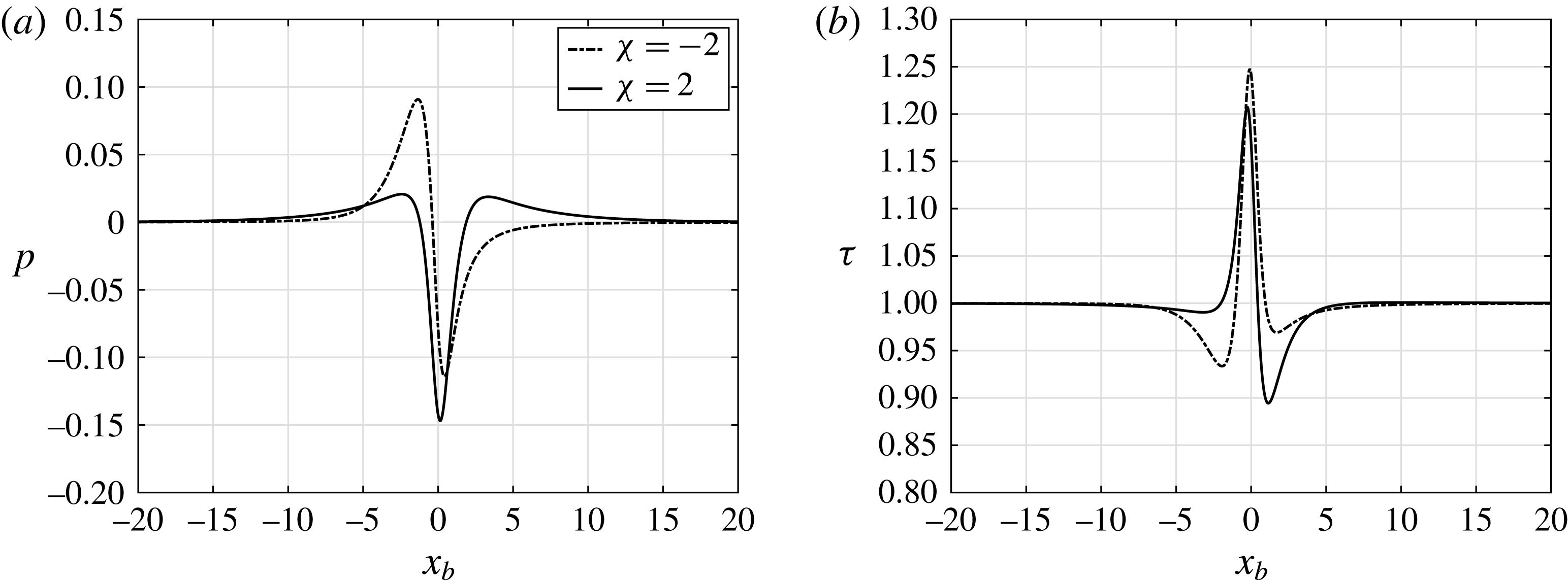
In figure 14(a,b) we have compared the results for the flow over the same hump shape
 $H(x)=h/(1+x^{2})$
but for both the supersonic flow with
 $\unicode[STIX]{x1D712}=-2$
and the subsonic flow
 $\unicode[STIX]{x1D712}=2$
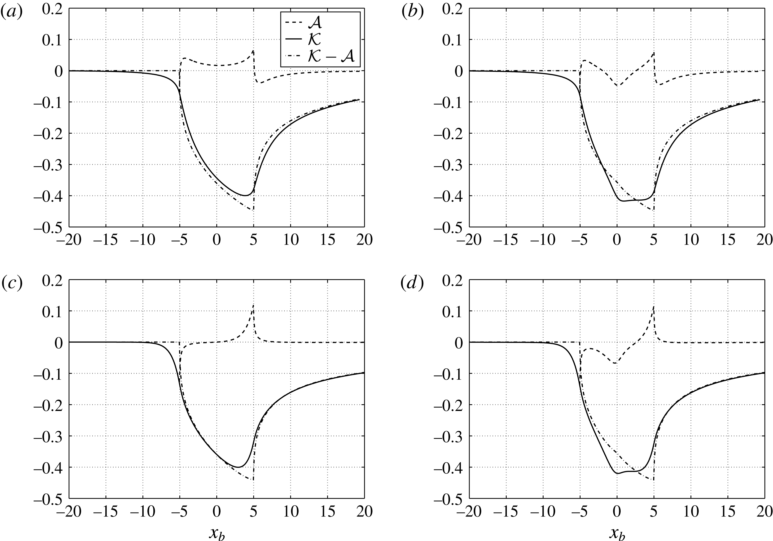
. For the supersonic flow, there is a stronger adverse pressure gradient ahead of the hump and heated region as compared to the subsonic case. As figure 13 (and other results presented earlier) shows, once the heating starts the flow becomes strongly attached over the hump but the shear drops once the top of the hump is overcome. In the subsonic case, the dip in the wall shear is much larger behind the hump. This again suggests that for heated humps in supersonic flow, the flow is more likely to separate ahead of the hump, whereas for subsonic flow it is more likely to separate behind the hump. In figure 15 we show plots of the displacement functions
 ${\mathcal{A}}$
,
 ${\mathcal{K}}$
and the contribution from the temperature perturbation term given by
 $$\begin{eqnarray}\displaystyle {\mathcal{K}}-{\mathcal{A}}=\int _{0}^{\infty }(1-T_{b}(x_{b},\unicode[STIX]{x1D702}))\,\text{d}\unicode[STIX]{x1D702}. & & \displaystyle\end{eqnarray}$$
Graphically these look similar to the plots presented by Koroteev & Lipatov (Reference Koroteev and Lipatov2012) in figure 3 of their paper except that the labels corresponding to the ‘Convective contribution’ and the
 $A(x_{b})$
label may be incorrect. In fact from our results the
 ${\mathcal{A}}$
contribution looks similar to what is labelled the ‘Convective contribution’ and the
 ${\mathcal{K}}$
contribution looks like the term labelled
 $A(x_{b})$
. Notice that the temperature contribution appears to be close to zero before the start of the heated region but is the largest in magnitude over most of the heated section. In figure 15 results are shown for both the flat-plate case with
 $h=0$
and the hump-shaped element with
 $h=0.1$
as well as for
 $\unicode[STIX]{x1D712}=\pm 2$
. The shape of the hump has a more substantial effect on the displacement function
 ${\mathcal{A}}$
for both
 $\unicode[STIX]{x1D712}=\pm 2$
whereas the temperature contribution looks very similar for all the cases presented in the figure.
Results for the unheated case with
 $\unicode[STIX]{x0394}T=0$
and the hump shape
 $H(x)=h/(1+x^{2})$
with
 $h=0.5$
and
 $\unicode[STIX]{x1D712}=\pm 2$
. (a) Pressure and (b) wall shear.

Plots of the displacement functions
 ${\mathcal{A}},{\mathcal{K}}$
and the temperature contribution
 ${\mathcal{K}}-{\mathcal{A}}$
for the heated hump
 $H(x)=h/(1+x^{2})$
with
 $a=10$
and
 $\unicode[STIX]{x0394}T=0.2$
. (a)
 $h=0$
and
 $\unicode[STIX]{x1D712}=2$
, (b)
 $h=0.1$
and
 $\unicode[STIX]{x1D712}=2$
, (c)
 $h=0$
and
 $\unicode[STIX]{x1D712}=-2$
and (d)
 $h=0.1$
and
 $\unicode[STIX]{x1D712}=-2$
.

5 Conclusion
We have formulated the problem of transonic flow past a heated hump-shaped element and new results have been presented. In addition to the height of the element and the strength of the wall temperature perturbation, another important factor that influences the flow significantly is the Kármán–Guderley parameter
 $\unicode[STIX]{x1D712}$
. The nonlinear coupling problem between the upper and lower decks is treated successfully using a hybrid finite difference and spectral numerical method. The results presented show the differences in behaviour between subsonic and supersonic flows as the height of the hump and strength of the heating element temperature are varied. As with previous work, supersonic zones embedded in a predominantly subsonic flow have been realised. Our results for the unheated hump-shaped elements compare well with those of Turkyilmaz (Reference Turkyilmaz2010) as well as with those presented by Diesperov & Korolev (Reference Diesperov and Korolev2003) as far as the pressure and wall shear are concerned, although there are slight differences in the shape of the displacement function with Diesperov & Korolev (Reference Diesperov and Korolev2003).
For supersonic flows, strong wall heating may lead to a separated flow before the element is reached, unlike subsonic flows in which the flow is more susceptible to separation behind the element. Under the same conditions, flows are more likely to separate in the transonic regime as compared to the subsonic or supersonic regimes. For flat-plate elements, the maximum values of the pressure are located at the start of the heating region, the pressure minimum at the end of the heated region, and the maximum values and minimum values increase in magnitude with increased wall heating. For flat-plate elements the pressure drop is monotonic in the heated region.
Heated hump-shaped elements as opposed to flat-plate heated elements, generate larger changes in the pressure and wall shear in the vicinity of the peak of the hump height. The pressure distribution is no longer monotonic in the heated region for hump-shaped elements.
Our results show that a heated hump-shaped element does slightly reduce separation in comparison to the unheated case. Computations with stronger heating were found to be difficult and computationally intensive because of the mixed-type flow occurring in the outer region, and hence were not pursued further, but it would useful to test whether even stronger heating can eliminate the separated zone which is present in the unheated case.
This study has concentrated on steady aspects only, and it is important to extend the work to look at unsteady aspects as well and assess how an array of humps could be used to exercise flow control.
Acknowledgements
Professor F. T. Smith FRS is thanked for his helpful comments. All the referees are thanked for their helpful and constructive comments on an earlier draft of the manuscript.