

INTRODUCTION
Tef (Eragrostis tef (Zucc.) Trotter) originated in Ethiopia (Vavilov, Reference Vavilov1951) and is one of the important cereal crops that grows in diverse climatic and edaphic zones of the country. The crop occupies 28% of the total cultivated area for cereals and accounts for about 21% of the total cereal production (Central Statistical Agency of Ethiopia (CSA), 2010). Tef grain is predominantly produced by smallholder farmers and about 62% of the population depend on it as staple food (Kebebew Assefa, 2011, personal communication). It provides about two-thirds of the dietary protein intake for most Ethiopians, who use tef as staple food (Seyfu, Reference Seyfu1997). The grains are highly nutritious and have a protein content of 9–11%, which is slightly higher than that of sorghum (Sorghum bicolour), maize (Zea mays L.) or oats (Avana sativa L.) (National Research Council (NRC), Board on Science and Technology for International Development 1996). Moreover, the grains are gluten-free, making them a valuable food source for people with celiac disease. Although tef follows the C4 photosynthetic pathway (Seyfu, Reference Seyfu1997), its low light utilisation, which could be associated with its small leaf size and specific leaf orientation, leads to limited photosynthetic efficiency (Dejene, Reference Dejene2009).
In semiarid areas, like in the northern highland of Tigray, agriculture is dependent on rainfed (RF) conditions, where the spatial and temporal variability of rainfall and occurrences of dry spell during seasons and in-between seasons are common. As a result of drought stress and other stress factors, the regional average yield of cereals and tef is oscillating around 1.4 t ha−1 and 0.93 t ha−1 (Central Statistical Agency of Ethiopia (CSA), 2000–2010), respectively. The water stress particularly at the later development stage of crops affected tef productivity as the result of earlier cessation of the rainfall. Dejene (Reference Dejene2009) reported that water stress during this period caused greater reduction in net CO2 assimilation and transpiration rates suggesting the need for supplementary irrigation to make up for the deficit in the seasonal rainfall.
Crop water productivity models can assist in understanding the effect of different physiological mechanisms to water stress (Geerts and Raes, Reference Geerts and Raes2009). AquaCrop (Raes et al., Reference Raes, Steduto, Hsiao and Fereres2009; Steduto et al., Reference Steduto, Hsiao, Raes and Fereres2009) can be used for this purpose as a tool to predict yield loss due to water stress. Furthermore, it supports to design management strategies like developing guidelines related to water management and developing scenarios for future climatic conditions. The model keeps a good balance between accuracy and relatively limited input requirements and was successfully calibrated for common crops such as maize and cotton (Garcia Vila et al., Reference Garcia Vila, Fereres, Mateos, Orgaz and Steduto2009; Heng et al., Reference Heng, Hsiao, Evett, Howell and Steduto2009) and for underutilised crops such as quinoa (Geerts et al., Reference Geerts, Raes, Garcia, Miranda, Cusicanqui, Taboada, Mendoza, Huanca, Mamani, Octavio, Mamani, Morales, Osco and Steduto2009).
The research for this study was carried out in Tigray, the northernmost region of Ethiopia, regarded as one of the most important regions for tef production in the country. The rainfall pattern in Tigray is unimodal with a clear-cut rainy season that occurs principally in July and August (Nyssen et al., Reference Nyssen, Vandenreyken, Poesen, Moeyersons, Deckers, Haile, Salles and Govers2005). The crop water productivity, which refers to the ratio of biomass produced over water transpired, of this rather unknown crop was modelled to gain insight into its physiological response to water stress. In this paper, we discuss the calibration and validation of AquaCrop for tef. In four successive years, field experiments were carried out at three locations in Tigray region, under RF and irrigation treatments, with both local and improved tef varieties. Preliminary yield response of tef to water stress has been investigated by Araya et al. (Reference Araya, Keesstra and Stroosnijder2010). They analysed only two growing seasons and used all the observed data for both calibration and validation of the AquaCrop model. By analysing our own data, this paper confirms, partly adjusts and completes the findings of Araya et al. (Reference Araya, Keesstra and Stroosnijder2010) and discusses some of the remaining physiological uncertainties.
MATERIALS AND METHODS
Model description
AquaCrop simulates green canopy (for water transpiration) and root growth (for water uptake) under the governing environmental conditions (Raes et al., Reference Raes, Steduto, Hsiao and Fereres2009). In exchange for water transpired, biomass is produced. Cumulative aboveground biomass production (B) is a function of the daily ratio of crop transpiration (Tr) and reference evapotranspiration (ETo) (Equation (1)). Yield (Y) is calculated by multiplying the final B by the harvest index (HI) (Equation (2)),
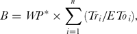

where B is the cumulative aboveground biomass production (g m−2); WP* is the normalised crop water productivity (g m−2); Tri is the daily crop transpiration (mm day−1); EToi is the daily ETo (mm day−1); n is the sequential days spanning the period when B is produced; Y is the yield production (g m−2); and HI is the harvest index (Raes et al., Reference Raes, Steduto, Hsiao and Fereres2009).
The proportional factor WP* in Equation (1) is the water productivity normalised for the local climate (expressed by ETo) and CO2 concentration (Steduto et al., Reference Steduto, Hsiao and Fereres2007). The main features of the AquaCrop model that differentiate it from other crop models is its focus on water, the use of ground cover instead of leaf area index and the use of water productivity values normalised for evaporative demand and CO2 concentration (Raes et al., Reference Raes, Steduto, Hsiao and Fereres2009). Simulations in the AquaCrop model need site-specific (climate, soil and management) and crop-specific (plant density, crop development, rooting depth, HI, crop coefficient (Kc) and water productivity) input parameters to make yield estimation. A detailed description of the model can be found in Steduto et al. (Reference Steduto, Hsiao, Raes and Fereres2009) and Raes et al. (Reference Raes, Steduto, Hsiao and Fereres2009), who describe the underlying principles and distinctive components, as well as the structural details and algorithms of the AquaCrop model, respectively.
Determination of water productivity (WP *) for tef in mini-lysimeters
The experiment was carried out at Mekelle University (MU) campus (13.30 ° N, 39.29 ° E, 2212 m above sea level (asl)) in 21 aboveground free-draining mini-lysimeters. The mini-lysimeters had a diameter of 0.21 m and a height of 0.33 m. Local variety of tef was broadcasted at a seed rate of 30 kg ha−1, which equals a population density of approximately 2000 plants m−2. The crop was grown from 22 November 2008 to 3 March 2009 in the mini-lysimeters containing cambisol. Urea and diammonium phosphate (DAP) were applied at a rate of 60 kg ha−1 (N and P2O5) as a source of nitrogen and phosphorus. All mini-lysimeters were placed under a rain shelter and arranged in a completely randomised design. Water was applied every other day to keep the water content in mini-lysimeters close to field capacity (FC), i.e. 36.6 vol%. If water drained out of mini-lysimeters, it was re-applied. The required amount of water was determined by calculating a soil water balance according to Allen et al. (Reference Allen, Pereira, Raes and Smith1998).
In six out of the 21 mini-lysimeters, tef was well watered, actively growing, completely shading the ground and regularly clipped to keep it at a uniform height of 0.12 m. As such, it was used as a hypothetical reference crop for ETo as mentioned by Allen et al. (Reference Allen, Pereira, Raes and Smith1998). The clipped plants were kept aside and no micro-climate, distorting ETo was generated. Since the crop covered most of the mini-lysimeters, evaporation was assumed negligible. These mini-lysimeters were used as a reference to determine the evaporating power of the atmosphere (ETo) for the environment.
On the other hand, the actual evapotranspiration (ETa) was determined from tef freely growing in the other 15 mini-lysimeters. To keep the transpiring surface exactly same as the surface of the mini-lysimeter and thus to minimise the error, overhanging tef plants were forced to grow straight with supporting sticks and slightly tied threads. Both ETa and ETo were determined every other day by measuring the mass difference of the lysimeters and the volume of applied water. The cumulative ratio of ETa over ETo (∑(ETa/ETo)) was calculated as a proxy for the cumulative ratio of transpiration normalised for climate, assuming the evaporation is negligible. Three replicates of intermediate B harvests taken at five successive points in time from 15 lysimeters were used to determine the normalised water productivity (WP*) of the crop as the linear regression between ∑(ETa/ETo) and the corresponding B (Steduto et al., Reference Steduto, Hsiao and Fereres2007). For these calculations, ETa was assumed equal to simulated transpirated water by the crop (Ta). Since nearly all the evaporation losses were limited to the initial season before canopy closure, which occurred very early, the slope of the curve between B and ∑(ETa/ETo) is a valid proxy for WP*.
Field experiments
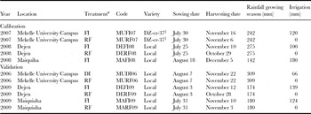
Study site and experimental design:. Field experiments (Table 1) were performed during the main rainy season for four years: (i) in 2006 and 2007 at MU, and (ii) in 2008 and 2009 at two sites located in east (Maiquiha, 13 °48′ N, 39 °27′ E, 2078 m asl) and southeast (Dejen, 13 °20′ N, 39 °22′ E, 2128 m asl) Tigray. An improved (Dz-Cr-37 in 2007) and local (in 2006, 2008 and 2009) varieties of tef were sown by the broadcast method with a seed rate of 30 kg ha−1. Recommended rates of nitrogen and phosphorous (P2O5) 60 kg ha−1 each for heavy and 40 kg N ha−1 and 60 kg P2O5 ha−1 for light soils. (Ethiopian Agricultural Research Organization (EARO), 2002) were applied in the form of urea and DAP. The urea application was split: 50% was given at sowing and the remaining 50% at tillering. DAP was applied at sowing. The crops were regularly weeded and protected against pests and diseases throughout the growing seasons.
Field experiments for the calibration and validation of AquaCrop for tef.
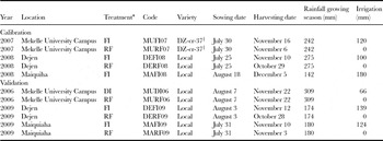
* FI: fully irrigated; RF: rainfed; DI: deficit irrigation: irrigated during flowering.
† Improved variety.
Rainfed, fully irrigated (FI) and deficit irrigation (DI, where irrigation was only applied during flowering) treatments were arranged in randomised complete block design with three (MUFI07, MURF07, DEFI08, DERF08, DEFI09, DERF09, MAFI08, MARF08, MAFI09 and MARF09) or four (MURF06 and MUDI06) replications (see Table 1 for codes). The size of the experimental plots was 9 m2 and 18 m2 in MU in 2006 and 2007, respectively, 4 m2 and 6 m2 in Dejen in 2008 and 2009, respectively and 4 m2 and 9 m2 in Maiquiha in 2008 and 2009, respectively. The spacing between the experimental plots was 0.5 m and the replications were 1.0 m apart from each other.
Measurements:. Climate data. Daily maximum and minimum air temperature, average wind speed at 2 m height, average percentage of relative humidity and hours of bright sunshine were recorded at the experimental sites and at a nearby agro-meteorological station to calculate ETo with the FAO Penman–Monteith equation (Allen et al., Reference Allen, Pereira, Raes and Smith1998). Daily rainfall was recorded at each site.
Soil data. The initial SWC of the experimental plots was measured gravimetrically (three replicates) on the respective sowing dates. The SWC in the root zone was measured gravimetrically every week at two depths between 0 and 0.4 m (Maiquiha; MU in 2006) or three depths between 0 and 0.6 m (Dejen; MU in 2007) from sowing till harvest in each experimental plot (three replicates, or four in MU in 2006).
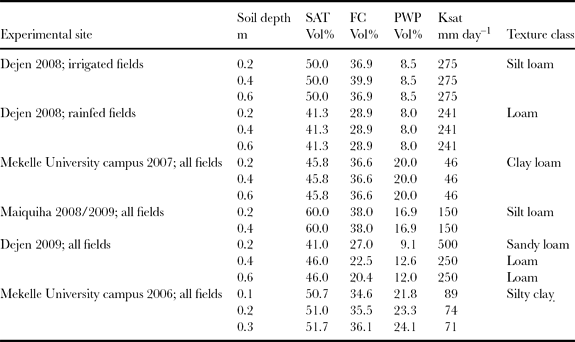
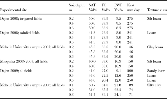
Soil samples (three replicates) of various fields were analysed in the laboratory to determine particle size distribution (by the hydrometer method). The SWC at saturation (SAT), field capacity (FC) and permanent wilting point (PWP) was determined using a pedotransfer function (Saxton and Rawls, Reference Saxton and Rawls2006). The soil physical characteristics are reported in Table 2.
Soil physical parameters at various depths for experimental sites.
Crop data. The time (in days after sowing) to reach different development stages (emergence, maximum canopy cover (CC), flowering, senescence and physiological maturity) was recorded during each growing season. The plant population density was counted using a 0.25 m × 0.25 m quadrant. The plant density for all experiments and all treatments was approximately 2000 plants m −2.
Green crop CC was determined every 10–15 days by taking digital pictures perpendicular to the experimental plot at an approximate height of 1.5 m. The pictures of an area (2.52 m2) were first resized to confirm uniform pixel size (1000 × 1000 pixels). To reduce the error that could occur at the four corners due to deformation (viewing angle), the centre square was selected as the most representative part of each picture and was subjected to the pixel analysing software SigmaScan Pro 5.1 (SPSS Inc., 1990–2000). With the help of the Turf-analysis macro (Karcher and Richardson, Reference Karcher and Richardson2005), the software counted the amount of ‘green’ pixels against the total amount of pixels. The three replicates of each treatment were used to determine CC in percentage.
The cumulative aboveground biomass production (B) during the season was measured at an interval of 10–15 days by cutting the plant from a quadrant of 0.25 × 0.25 m2 for the 4 m2 and 6 m2 plot sizes, and a quadrant of 0.5 × 0.5 m for the 9 m2 and 18 m2 plot sizes and was dried for 48 h at 65 °C in a ventilated oven. In Maiquiha in 2008, only the final B and final Y were recorded. Final Y and final B at harvest were taken from a quadrant of 2.5 m2 and 3.68 m2, respectively for the smaller (4 or 6 m2) and 6 m2 for the larger plot size (9 or 18 m2). The HI was calculated as the ratio of final Y to final B.
Management. Supplementary irrigation for full and DI treatments was applied by flooding small basins. The timing and depth of the irrigation applications were determined by means of a soil water balance (Allen et al., Reference Allen, Pereira, Raes and Smith1998). In the calculation, the crop evapotranspiration (ETc) was determined with the Kc × ETo approach. A Kc of 1.1 was used, which is a good indicative value for small cereals with good soil cover after development.
Calibration and validation of AquaCrop for tef
The determined WP* within the mini-lysimeters and the observations of the field experiments in 2007 and 2008 at three locations were used to calibrate the AquaCrop model. In the calibration process, the observed time (in calendar days) to developmental stages (emergence, maximum CC (100%), flowering, senescence and physiological maturity) under well-watered conditions (FI treatments) were used to describe crop development under non-limiting conditions in AquaCrop. Subsequently, water stress coefficients (Ks) for leaf expansion, stomata closure and early canopy senescence were calibrated on the basis of the physiological characteristics of the crop and in an iterative way by comparing observed CC and SWC with the simulated outputs of AquaCrop for FI and RF treatments. The default shape of the Ks curves, which determines the magnitude of the effect of soil water stress factors, was retained (Raes et al., Reference Raes, Steduto, Hsiao and Fereres2009). The reference HI and parameters describing the effect of water stress on the HI were calibrated with data from FI and RF treatments. The observations of CC, SWC, B and Y were used as benchmarks during the calibration process. Calibrations started with tef under FI (no water stress). Subsequently, tef under RF conditions was considered.
Calibration and validation were evaluated for SWC, CC, B and Y by comparing simulated outputs with data collected from the field using the following statistical parameters: (i) R 2, which quantifies the portion of the total observed variance that can be explained by the model; (ii) the root mean square error (RMSE), which expresses the overall mean deviation between the observed and simulated values as a measure for the relative model uncertainty (Loague and Green, Reference Loague and Green1991); (iii) the index of agreement (d, Willmott, Reference Willmott1982), which shows differences in the observed and predicted means and variances and (iv) EF (Nash and Sutcliffe, Reference Nash and Sutcliffe1970), which assesses the overall deviation between the observed and simulated values to the variability of observations as a measure of the model performance over the whole simulation period. Better model performance is achieved when R 2, EF and d approach unity and when RMSE approaches zero.
RESULTS
Water productivity (WP*) for tef derived from lysimeter experiments
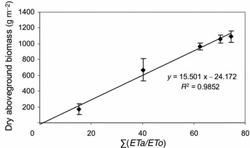
The water productivity of tef in the lysimeter experiment was determined from the linear regression between the cumulative ratio of observed dry aboveground biomass and cumulative ratio of transpiration over ETo. As clearly presented in Figure 1, there is a linear increase of observed biomass as a function of the cumulative ratio between transpiration adjusted for ETo (R 2 = 0.98). The experimentally determined WP* for tef was 15.5 g m−2 (Figure 1).
Water productivity of tef (local variety) from the lysimeter experiment based on cumulative normalised evapotranspiration versus dry aboveground biomass. Error bars represent standard deviations (n = 3).

Calibration of AquaCrop for Tef
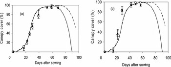
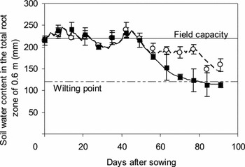
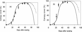
Examples of the simulated and observed CC and SWC for RF and FI treatments are presented in Figures 2 and 3. Regardless of the year and the location of the experiment, the observed and simulated CC development fitted well (Figures 2a and 2b) and followed the standard logistic growth curve used by AquaCrop for non-stressed conditions (Raes et al., Reference Raes, Steduto, Hsiao and Fereres2009). The maximum CC of about 100% was reached in 49 days after sowing in the experiments of 2007 and 2008.
Observed (symbols with error bars of standard deviation (n = 3)) and simulated (lines) canopy cover for rainfed (solid squares, full line) and fully irrigated (open circles, dotted line) treatments for (a) Mekelle University campus 2007, (b) Dejen 2008.
Observed (symbols with error bars of standard deviation (n = 3)) and simulated (lines) soil water balance for rainfed (solid squares, full line) and fully irrigated (open circles, dotted line) treatments for Mekelle University campus 2007.
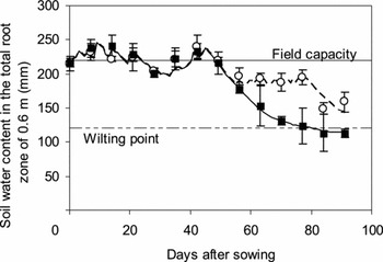
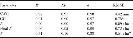
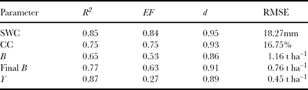
In the RF treatment, both simulated and observed CC (Figure 2) and SWC (Figure 3) dropped very quickly after the rains ceased, indicating the shorter crop cycle of RF tef due to early senescence. Table 3 shows the statistical parameters for the fit with high R2, EF and d values except for the low EF of the yield. The low values of RMSE indicate that the overall deviation between the model simulations and observations was limited for all the computed parameters.
Goodness of fit analysis for the simulation of soil water content (SWC), canopy cover (CC), biomass (B; which includes intermediate and final biomass), final biomass (final B) and yield (Y) after calibration of AquaCrop for tef.
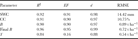
R 2: coefficient of determination; EF: Nash–Sutcliffe efficiency; d: index of agreement; RMSE: root mean square error (all values are averaged over different fields and for the time series of SWC, CC and B).
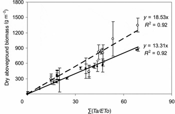
Observed values for B from field experiments were plotted against the cumulative ratio between Ta and adjusted ETo in Figure 4. The slope of the linear fit allowed to draw WP* of both improved and local varieties of tef valued 18.5 g m−2 and 13.3 g m−2, respectively. R2 for the WP* determined in the field for both varieties was 0.92, indicating that there is excellent correlation between the cumulative normalised transpiration and B.
Water productivity of tef grown under field conditions based on cumulative normalised transpiration versus dry aboveground biomass for improved variety (open circles, dotted trend line) and local variety (solid squares, full trend line). Error bars represent standard deviations (n = 3).
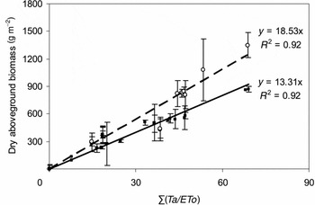
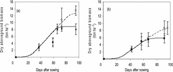
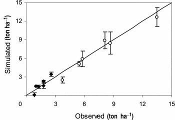
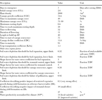
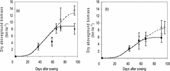
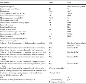
A WP* of 14 g m−2 was selected for the local variety by considering the results from the lysimeters (WP* = 15.5 g m−2) and the field experiments (13.3 g m−2). A WP* of 21 g m−2 was selected for the improved varieties, assuming (i) a similar deviation as for the local varieties between the realistic WP* and the value from field experiments (WP* = 18.53 g m−2) and (ii) by giving more weight to the final B (where sample sizes are larger than for intermediate B) during the final calibration of the model. After the selection of WP* and a reference HI (HIo) of 27%, good simulation for B and Y could be obtained. Figure 5 shows examples of simulated and observed B for RF and FI treatments. The simulations fitted the observed data very well with higher B attained from irrigated treatment in both locations and years. The regression between the observed and simulated final B and Y for all data sets used for calibration are given in Figure 6, indicating R 2 = 0.84 and 0.96 for Y and B, respectively. The crop parameters for tef obtained after calibration are listed in Table 4.
Observed (symbols with error bars of standard deviation (n = 3)) and simulated (lines) dry aboveground biomass for rainfed (solid squares, full line) and fully irrigated (open circles, dotted line) treatments for (a) Mekelle University campus 2007 and (b) Dejen 2008.
Regression between observed and simulated yields (solid diamonds, R 2 = 0.84) and final dry aboveground biomass (open circles, R 2 = 0.96) with error bars of standard deviation (n = 3) for all calibrated treatments.
Calibrated crop parameters for tef in AquaCrop.
Validation of the calibrated model
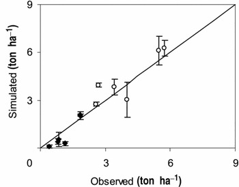
The validation of the model was carried out by considering the calibrated crop parameters (Table 4) and data sets from field observations in 2006 and 2009 at three sites and for three treatments (FI, RF and DI). Observed SWC in the root zone, green CC, B and Y were compared with the validated result of simulation. Table 5 gives an overview of the statistical parameters for the validation of the AquaCrop model. The parameters confirmed good match between simulations and observations.
Goodness of fit analysis for the simulation of soil water content (SWC), canopy cover (CC), biomass (B; which include intermediate and final biomass), final biomass (final B) and yield (Y) for the validation of AquaCrop for tef.
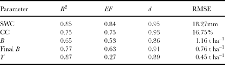
R 2: coefficient of determination; EF: Nash–Sutcliffe efficiency; d: index of agreement; RMSE: root mean square error (all values are averaged over different fields and for the time series of SWC, CC and B).
DISCUSSION
The experimentally determined WP* of tef from the lysimeter (Figure 1) and field experiments (Figure 4) demonstrates a linear increase of the observed biomass as a function of the cumulative ratio between transpiration and ETo, which confirms the hypothesis of the conservative behaviour of WP* as formulated by Steduto et al. (Reference Steduto, Hsiao and Fereres2007). The normalised WP* of the crop derived as the slope of the linear regression between ∑(ETa/ETo) and the corresponding B sampled periodically from both experiments did not level off during yield formation as is the case for sunflower by the production of highly nutritious seeds (Steduto and Albrizio, Reference Steduto and Albrizio2005). However, the estimated WP* of tef found from both experiments was very low for a C4 plant and contrasts with the WP* for other C4 crops: 32.9 g m−2 for sorghum (Steduto and Albrizio, Reference Steduto and Albrizio2005), 33.7 g m−2 for maize (Heng et al., Reference Heng, Hsiao, Evett, Howell and Steduto2009; Hsiao et al., Reference Hsiao, Heng, Steduto, Rojas-Lara, Raes and Fereres2009) and the indicative range (30–35 g m−2) given in AquaCrop (Raes et al., Reference Raes, Steduto, Hsiao and Fereres2010). The low WP* could be the consequence of a higher protein content of tef in comparison with other C4 crops, due to which the crop requires considerably more energy per unit dry weight to convert the assimilated CO2 into carbohydrates (Azam-Ali and Squire, Reference Azam-Ali and Squire2002). Its lower light use efficiency compared with other C4 plants, which is related to leaf size and orientation as mentioned by Dejene (Reference Dejene2009), could also explain the low WP*.
The evolution of the observed and simulated SWC in the root zone is plotted for the FI and RF treatments as shown in Figure 3, which indicate well-simulated Tr as a result of a very good match between simulations and observations for both treatments. This was confirmed by adequate values of the parameters used to evaluate the goodness of fit of the model (Table 3).
A calibration on crop characteristics was carried out to improve the simulations. Input values for different crop parameters given in Table 4 were based on observations with minimal adjustment. The evolution of the simulated values for CC over time for RF and FI tef showed a very good comparison with the observed values (Figures 2a and 2b). This result shows that the thresholds for root zone depletion at which water stress affects canopy development (p exp), induces stomata closure (p sto) and triggers early canopy senescence (p sen) were well selected.
By making use of the observed HI and a selection of WP* for both local and improved varieties of tef, satisfactory grain yield simulation was observed (Figure 6), suggesting that AquaCrop correctly simulated the effect of water stress during different phenological stages on the HI of tef. Depending on the magnitude of water stress during yield formation, HIo in AquaCrop might be adjusted upward or downward. Stresses affecting only leaf expansion have a positive effect on HI, while more severe stresses inducing stomata closure have a negative effect on HI. In AquaCrop, HIo can also be adjusted to water stress occurring before and during flowering.
For tef, water stress affected the HIo in the following way:
1. As there was no or very mild water stress before flowering for all experimental years, the positive effect of pre-flowering water stress on HIo of tef could not be considered.
2. The data analysis revealed that tef is very tolerant to water stress during flowering. A high depletion of total available soil water (TAW) was selected (p upper = 0.92) for the water stress affecting pollination during flowering.
3. Simulations with AquaCrop indicated for tef that slight to moderate water stresses during yield formation increased HIo as a result of water stress affecting leaf expansion. This is due to the restriction of excessive vegetative growth during this growth stage, which means that more energy can be used for the production of yield.
4. The drop of HI due to strong water stress during yield formation as reported among many studies by Farré and Faci (Reference Farré and Faci2006) for maize and sorghum and by Karunaratne et al. (Reference Karunaratne, Azam-Ali, Al-Shareef, Sesay, Jørgensen and Crout2010) for Bambara groundnut is a common physiological process. Simulations indicated that this is also present in tef for severe water stresses, although to a smaller extent.
The manifested positive effect of water stress on HI during yield formation and the relatively small negative effect during flowering and yield formation render tef to be a crop with unique characteristics. This may be the reason why farmers in areas prone to moisture stress use tef as a rescue crop in case of failure of other cereals (Seyfu, Reference Seyfu1997). It indicates its ability to withstand water stress, which is likely to occur when planting late in the rainy season after a crop failure.
From the statistical analysis of the simulation results (Table 3), it could be concluded that the main features of tef as affected by water stress were well modelled by AquaCrop. R 2 for all variables was ≥0.84 and d approached 1. The relative small RMSE and a good range of EF (≥0.90, except for yield) confirmed the goodness of fit between the observed and simulated results. The low EF value for the yield could be attributed to the underestimation of the yield by the model for RF tef in Maiquiha 2008. This may indicate that the model is less satisfactory in simulating crop growth and production in severe water stress conditions as was the case at this site in the dry year 2008 or it could also be an error in the measurements.
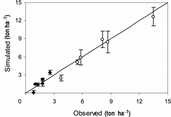
The validated SWC in the root zone of the crop was in good agreement with the observed values. This indicated that the calibration of AquaCrop for tef was satisfactory and ETc was well estimated. The model was able to appropriately simulate the development of CC and B. A correct calibration of the effect of water stress on HIo, by which HI increased from 27% in conditions without water stress to 33% in conditions with mild water stress, resulted in an accurate simulation of Y (Figure 7).
Regression between observed and simulated yields (solid diamonds, R 2 = 0.87) and final dry aboveground biomass (open circles, R 2 = 0.77) for validation fields. Error bars represent standard deviations (n = 3).

CONCLUSION
The simulations of the soil water balance and the development of green CC gave a good indication that AquaCrop is able to calculate Ta quite well. A good estimation of Ta is crucial to estimate yields, since biomass yield follows directly from the product of the WP* with the cumulative Ta adjusted for ETo. Notwithstanding the fact that tef is a rather unknown crop and by considering the physiological complexity of the crop responses to water stress, adequate results were obtained with AquaCrop with a relatively limited amount of crop parameters. In the current study, it was found that the common biomass water productivity for a C4 crop is far from that reached in tef.
The simulation of tef reported in this paper extended the preliminary calibration of Araya et al. (Reference Araya, Keesstra and Stroosnijder2010) for AquaCrop because it made a clear distinction between calibration and validation, and used an extensive data set of four years’ observations with three water treatments at three different locations on different soil types. Further on, a distinction was made between local varieties close to the wild type used by most farmers and improved tef varieties.
Given that AquaCrop keeps a good balance between accuracy and input requirements, it could be used to improve tef crop water productivity at its centre of origin through developing guidelines on the effective way of cultivating crops in terms of water management strategies. Moreover, as it is a useful tool to develop scenarios for future climatic conditions, estimated yield gaps between the potential and actual yields of a particular crop under its specific climatic and soil conditions can be useful to increase awareness for timely and quantitative information related to food relief measures. In addition, AquaCrop can serve as an explanatory model in the breeding programs of tef. Nevertheless, further studies have to be carried out to test the model with other management practices, including fertility stress effect, weed infestation effect and effect of sowing dates, as these are also important factors that limit tef productivity.
Acknowledgements
The authors are grateful to R. Reggers, N. Viaene, W. Raes and M. Garcia-Vila for their valuable effort in the collection and analysis of field data. This research project was funded by the Mekelle University–Institutional University Cooperation Programme (MU–IUC, VLIR UOS).