




No CrossRef data available.
Article contents
Mathematical and statistical analysis of the Trypanosoma brucei slender to stumpy transition
Published online by Cambridge University Press: 19 January 2004
Abstract
We propose a new model for the Stumpy Induction Factor-induced slender to stumpy transformation of Trypanosoma brucei gambiense cells in immunosuppressed mice. The model is a set of delay differential equations that describe the time-course of the infection. We fit the model, using a maximum-likelihood method, to previously published data on parasitaemia in four mice. The model is shown to be a good fit and parameter estimates and confidence intervals are derived. Our estimated parameter values are consistent with estimates from previous experimental studies. The model predicts the following. Slender cells can be classified as uncommitted, committed and dividing, and committed and non-dividing. A committed slender cell undergoes about 5 divisions before exiting the cell-cycle. Committed slender cells must produce SIF, and stumpy cells must not produce SIF. There are two mechanisms for differentiation, a background differentiation rate, and a SIF-concentration-dependent differentiation rate, which is proportional to SIF concentration. SIF has a half-life of about 1·4 h in mice. We also show, with suitable changes in the parameter values, that the model reflects behaviours seen in other host species and trypanosome strains.
Information
- Type
- Research Article
- Information
- Copyright
- 2004 Cambridge University Press
INTRODUCTION
African trypanosomes cause widespread disease in humans and livestock. They are transmitted between mammalian hosts by the bite of the tsetse fly. When first transmitted to a mammal, trypanosomes have a long, slender morphology and these forms are not infectious to the tsetse. Slender cells divide rapidly in the bloodstream and other organs before transforming into non-dividing stumpy forms. Stumpy cells are infectious to the tsetse.
Within a host, successive waves of parasitaemia are observed. As the host's immune system fights off one wave, trypanosomes change their antigenic coat and escape to start a new wave (Barry & Turner, 1991). However, the host's immune system is not the only mechanism that causes parasitaemic waves. Trypanosomes are able to regulate their own density by slender to stumpy cell differentiation when their density passes a critical threshold. It has been speculated that this is an evolved trait in order to keep the host alive for prolonged periods – a necessity when tsetse bites are infrequent (Vassella et al. 1997).
Black et al. (1985) and Seed & Sechelski (1989 b) first proposed that the slender to stumpy transformation is triggered by a cell density-sensing mechanism, and further work has supported this idea (Seed & Black, 1997; Reuner et al. 1997; Vassella et al. 1997; Seed & Black, 1999; Tyler et al. 2001). Hesse et al. (1995) first suggested that a trypanosome-derived factor or metabolite is the mediator of the density-sensing mechanism. Then, in a set of elegant experiments, Vassella et al. (1997) demonstrated that the factor is produced by the trypanosomes and that it acts via the cAMP pathway. They termed this factor SIF, short for stumpy induction factor. They also demonstrated that cell-cycle arrest precedes morphological change.
Several mathematical models have been proposed to describe slender to stumpy differentiation (Turner, Aslam & Dye, 1995; Seed & Black, 1997, 1999; Tyler et al. 2001). However, none has performed a rigorous statistical analysis on their fit to data. That is, they have not been tested for goodness-of-fit. Nor have their parameters been tested for significance and, in some cases, no confidence limits determined.
In this paper we propose a new model, based on elements of the previous models and extended to include SIF-induced differentiation. The model is fitted to data from previous experiments with immunosuppressed mice (Seed & Sechelski, 1988, 1989 a; Seed & Black, 1997). By removing the effects of the immune system we can get a better understanding of the density-sensing mechanism.
Our model is fitted, using the maximum-likelihood method, to reconstructed data from the experiments. This gives quantitative estimates of the model parameters. Such estimates give our model strong predictive capacity and the potential to be rigorously tested.
MATERIALS AND METHODS
Previous experiments
Five mice of strain C3HeB/FeJ were irradiated to suppress their immune systems (more details are available in Seed & Black (1997)). Each mouse was infected with 1000 or 5000 T. brucei gambiense cells of clone NCTat-1.36. At various times, the tail of each mouse was snipped and a drop of blood obtained. The blood was diluted in 1% glucose phosphate-buffered saline plus 1% sodium citrate (GPBS+C) as an anticoagulant. Whole blood was diluted 1 part blood to 49 parts GPBS+C. If the number of trypanosomes in this suspension was too high to read, further dilutions were made. Two aliquots from each mouse were analysed in a haemacytometer. A second drop of tail blood was smeared on a glass slide, stained with Giemsa, and a minimum of 100 trypanosomes were examined for their morphological type.
One mouse died prematurely so we will not use its data in this paper.
Reconstructing the original data
Unfortunately, the original cell counts from the haemacytometer and staining experiments have been lost. To do a statistical analysis based on the maximum-likelihood method we need to reconstruct these lost cell counts. Fortunately, this is possible because we know the experimental procedure.
The data consist of total cell concentrations and three cell-type concentrations – slender, intermediate and stumpy – at various times. The concentrations are measured in units of number of cells per millilitre of blood. Due to problems of distinguishing between intermediate and stumpy cells we combine these two classes into a single stumpy class.
To reconstruct the total cell counts let us define d to be the dilution made, vs to be the volume of the dilution counted in the haemacytometer and r to be the number of aliquots. The total volume of blood analysed is, therefore, v=rvs/d. If nt is the total number of cells counted then the expected total concentration of cells in the blood is Ĉt=nt/v. We want to find nt having been given v and Ĉt. Therefore

where nt is rounded to the nearest integer.
To reconstruct the counts for the two cell-types let us define mt to be the total number of cells counted. Let nl and ns be the counts of slender and stumpy cells respectively. The expected frequencies of the cell-types are

and

. The expected concentrations of the two types are, therefore,

and

. We want to find nl and ns having been given mt, Ĉl, Ĉs and Ĉt. Therefore

where i is l or s, and ni is rounded to the nearest integer.
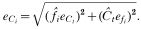
As well as reconstructing the cell counts we can calculate the standard errors in the expected total cell concentrations and the cell-type frequencies and concentrations. Although these are not needed for the statistical analysis, they are instructive when plotting the data.
There are two main sources of error in the experiments. The first is due to the difficulty of counting highly motile cells in a haemacytometer. Cells may be counted more than once or not at all if they migrate into adjacent squares. This source of error was minimized by counting a slide 2 or 3 times and taking an average count, and by the same experienced person examining all the slides. In our analysis, we assume that this error is negligible. The second source of error is a sampling error, which we can calculate as follows.
The standard error of the estimated total cell concentration is

A detailed derivation of this equation, and the ones that follow, are given in Appendix A. The standard errors of the estimated frequencies are

where i is l or s. Thus the standard errors in the estimated concentrations of the two cell-types are
The model
The model is a set of delay differential equations (DDEs) that describe how the cell and SIF concentrations change over time. We define the model's variables and parameters in Table 1, and a schematic representation of the model is shown in Fig. 1.

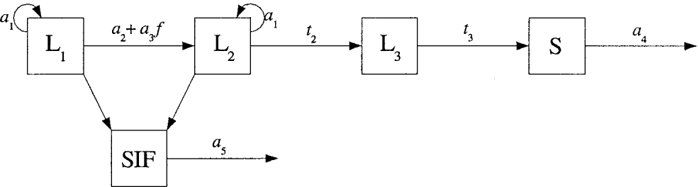
Fig. 1. Schematic representation of the model. Slender cells, denoted L, are split into 3 subclasses: those not committed to differentiate, denoted L1, those committed to differentiate but still dividing, denoted L2, and those committed to differentiate and not dividing, denoted L3. Stumpy cells are denoted S. The parameters are defined in Table 1 and the model details are given in the text.
The model equations are
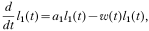



where

is the differentiation rate of uncommitted slender cells. The initial conditions are


Because we are assuming that no differentiation occurs before time t1 (see below), we do not need to specify conditions before this time.
The model is based on the following assumptions. (1) The cells and SIF are well-mixed in the blood. (2) The influx and outflux of cells between the blood and any other organs infected by trypanosomes is in equilibrium, that is, can be ignored. (3) The injected slender cells do not immediately begin to differentiate or grow exponentially. Only after t1 h does the slender cell population begin to grow exponentially, produce SIF and differentiate. The concentration of uncommitted slender cells is set to c1 cells/ml at this time. (4) Slender cell birth rate is proportional to the instantaneous, dividing slender cell concentration l1+l2. This gives exponential growth of the slender cell population as observed experimentally. The birth rate is a1, and the population doubling time, in the absence of differentiation, is given by ln(2)/a1. (5) On receiving the differentiation signal, the transitions from one class to the next take fixed periods of time. The uncommitted (L1) to committed slender cell (L2) transition is instantaneous. The dividing committed to non-dividing committed slender cell (L3) transition takes t2 h. The non-dividing slender cell to stumpy cell (S) transition takes t3 h. So, once a slender cell is committed to differentiate, it can take several hours for it to become recognizable as a stumpy cell. (6) Because there is a time lag between receiving a differentiation signal and exiting the cell-cycle, a committed slender cell may have many descendants. We assume that all descendants are also committed to differentiate. (7) Stumpy cell death rate is proportional to the instantaneous stumpy cell concentration. The death rate is a4 and the half-life in hours is given by ln(2)/a4. (8) SIF is produced at a rate proportional to the instantaneous concentration of dividing slender cells. We do not know the production rate of SIF, nor do we know at what concentration it induces differentiation. Therefore, we can normalize the production rate to 1, giving us one less parameter to fit (see Appendix B). (9) SIF degrades exponentially at a rate a5. Its half-life in hours is given by ln(2)/a5. (10) There is a background level of differentiation of slender cells, irrespective of SIF concentration. This is necessary because we observe stumpy cells at all times, in particular, during the exponential growth phase. This background rate is constant and occurs at a rate a2. (11) As cell concentration reaches about 108 cells/ml there is a marked increase in the differentiation rate. We must assume something about the functional form for this differentiation rate. The simplest form is linear: that is, proportional to SIF concentration. Another, more biologically motivated mechanism, is described by Michaelis–Menten kinetics. This has the form

where a3 is the maximum differentiation rate, and c2 the Michaelis–Menten constant. A sketch of this equation is shown in Fig. 2A (solid line). As f increases, differentiation rate saturates at the value a3. Biologically, this can be interpreted as a saturation of membrane receptors by ligand (e.g., SIF) as the ligand concentration increases.
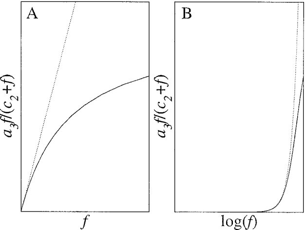
Fig. 2. Solid lines: (A) Michaelis–Menten kinetics of slender cell differentiation rate. (B) As SIF concentration is increasing exponentially, Michaelis–Menten kinetics gives switch like behaviour in the differentiation rate. The dotted lines represent differentiation rate proportional to SIF concentration i.e., a3f. For an exponentially increasing population, such a rate also gives switch-like behaviour.
Because the slender cell concentration and hence SIF concentration, increases exponentially, differentiation rate switches from background to above background very rapidly. This is demonstrated by the sketches in Fig. 2B by using a logarithmic x-axis.
Numerical schemes
A fourth-order Runge–Kutta scheme with fixed time-step h was used to solve the equations. To use this scheme we must convert our model from a finite set of delay differential equations to an infinite set of ordinary differential equations. The reformulated model is given in Appendix C. All numerical solutions were done with h=0·25. This was checked to make sure the solutions were stable and accurate.
Curve fitting
The model was fitted to the data using the maximum-likelihood method. For a particular set of parameters and data we calculate the likelihood of these parameters given the data. We then adjust the parameters in order to maximize the likelihood, thus giving us our maximum-likelihood parameter estimates. The likelihood is found as follows.
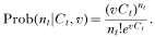
We know that, if the total cell concentration is Ct and if we analyse a volume v of blood in a haemacytometer then, the probability of counting nt cells is given by a Poisson distribution
We also know that, if the frequencies of the two cell-types are fl and fs then, the probability of counting nl and ns cells, given that we count mt cells in total, is given by a binomial distribution

The likelihood of a set of parameters given the data is proportional to the product of all the probabilities of the data given the simulated results of the model. That is,

where j denotes a particular data point. Ct, fl and fs are found by simulating the model for a particular parameter set. vj, mtj, ntj, nlj, nsj are the data at time tj.
For convenience the natural logarithm of the likelihood is calculated. The maximum-(log)-likelihood, lmax=ln(Lmax), is found using the Marquis–Levenberg algorithm (Press et al. 1992) with a tolerance of 10−6.
Statistical analysis
Goodness-of-fit.
Once the best-fit parameters for a particular data set have been found we want to test the goodness-of-fit of these parameters. We do this by comparing the observed maximum-likelihood (lmax) to its expected distribution. The expected distribution is found by simulating artificial data sets from the best-fit model. We can do this because we know the experimental procedure. We simulate 100 data sets and calculate their maximum likelihoods. These are then binned to create a distribution. The observed lmax is compared to its expected distribution. If the observed lmax falls above 5% of the values in the expected distribution then the parameters are considered a good fit. Otherwise they are considered a poor fit.
Parameter significance.
Parameter significance is tested by setting each one to zero and recalculating the maximum-likelihood. However, to test the significance of the initial slender cell concentration, c1 is set to 1000, otherwise there would be no cells in the blood. Significance is determined by using the likelihood-ratio test. If the difference between the original and recalculated maximum-likelihoods is greater than 1, then the parameter is significant at the 5% level.
Parameter error estimates.
To estimate the errors in the parameter values we assume that the best fit parameters to a particular data set are the true parameters. Using these parameters, we simulate 100 artificial data sets and calculate their maximum-likelihoods. This gives 100 sets of estimated parameters from which we can construct a probability distribution for each parameter.
RESULTS
The reconstructed data
In Tables 2 and 3 we tabulate the original and reconstructed data for each mouse. The total number of cells counted to determine the frequency of each type (mt) is unknown. Therefore, we assumed that 100 cells were counted for each case. The data and error bars for the four mice are shown in Fig. 3.

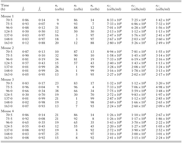

Fig. 3. Experimental results (circles) with error bars (±1 S.E.M.). One error bar extends to zero. The x-axis gives the time since the start of the experiment, and the y-axis the number of cells/ml on a log scale.
Best-fit curves
The best-fit curves for all mice are shown in Fig. 4. The maximum-likelihoods are tabulated in Table 4.

Fig. 4. Best-fit curves. Circles are observed values, lines are best fits. The x-axis shows time since beginning of experiment, the y-axis shows cell concentration in cells/ml on a log scale. Dotted lines for mouse 3 shows best-fit where cell type concentrations at 75·5 h have been omitted from the fit. Dotted lines for mouse 4 shows best-fit where total and cell type concentrations at 75·5 h have been omitted from the fit.
Goodness-of-fit
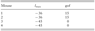
The goodness-of-fit of each mouse is given in Table 4.
The fits are good for mice 1 and 2, but very poor for mice 3 and 4. This might be caused by outliers in the data. For mouse 3, potential outliers are the stumpy cell concentrations at 70·5 and 75·5 h. For mouse 4, potential outliers are the slender and stumpy cell concentrations at 70·5 and 75·5 h.
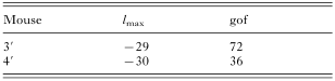
For mouse 3, removing the stumpy cell concentration at 75·5 h gives a much better fit (see Table 5 and the dotted lines in Fig. 4C). Removing the stumpy cell concentration at 70·5 h also gives a good fit (result not shown). For mouse 4, removing all data points at 75·5 h gives a much better fit (see Table 5 and the dotted lines in Fig. 4D). Removing all data points at 70·5 h also gives a good fit (result not shown). We denote these modified fits as corresponding to mouse 3′ and mouse 4′.
Parameter significance of the best-fit model
The maximum-likelihoods of the model with constrained parameters for all mice are shown in Table 6. Parameter significance for a particular mouse is denoted by a tick.

Parameters t1 and c1 set up the initial conditions. Parameter t1 is marginally significant, which probably implies that differentiation does not begin immediately at the start of the experiment, but it can be compensated for by changes in c1 during the fitting procedure. Parameter c1 is not significant: setting it to 1000 cells/ml can be compensated for by changes to t1. Parameter a1, the slender cell birth rate, is clearly significant. Parameter a2, the background slender cell differentiation rate is significant. This is because differentiation is taking place even before SIF concentration has reached levels high enough to limit the parasitaemia after 124·5 h. Parameter a3, the above-background slender cell differentiation rate, is highly significant. Without this parameter there would be no self-limitation of the parasitaemia, that is, only exponential growth. Parameter a4, the stumpy cell death rate, is only marginally significant in mouse 3′. This is because the drop in stumpy cell concentration is only captured by the last data point at 163 h. Parameter t2 is significant as without it there are no oscillations in slender cell concentration (see below). Parameter t3 is marginally significant as removing it only has a small effect on the dynamics. Parameter a5 is significant, as without SIF degradation the slender cell concentration would not recover after its drop.
Parameter estimates
The parameter estimates for each mouse are given in Table 7. In Fig. 5 we show boxplots of the parameter distributions. The median is shown as a horizontal line contained within a box that bounds 50% of the values. Small circles show outliers in the distributions. Even though the stumpy cell death rate is not a significant parameter, it is included because there is strong evidence that stumpy cells do die (Black, Hewett & Sendashonga, 1982; Turner et al. 1995).
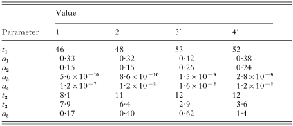

Fig. 5. Boxplots of the estimated parameter distributions. The horizontal line is the median, the box bounds 50% of the values. Circles show outliers.
Many of the parameters show discrepancies between mice 1 and 2 and mice 3′ and 4′. This is most likely due to the removal of the outliers at 75·5 h for mice 3′ and 4′. Parameter a4 is much smaller for mouse 1 than for the other mice. This is because the stumpy cell concentration in this mouse does not fall near the end of the experiment as it does in the others.
There is quite a large variation in parameters a3 and a5. By de-dimensionalizing the model we can show that the differential equation describing SIF rate of change can be written as

Thus, changing a3 and a5 by an equal factor does not change the solution. For the best-fit model, a5/a3 varies from 3 to 5×10⁸ across the four mice. This is a much smaller variation than when the parameters are treated separately. This suggests that the variations in the separate parameters are an artifact of the fitting procedure and not true variations between the mice.
Having found our best-fit model we can now make some further predictions. We can calculate differentiation rate, extrapolate the simulations forward in time, and change parameter values and observe their effects on the dynamics.
Differentiation rate
We can determine the instantaneous differentiation rate of slender cells from class L1 to L2. This is given by a2+a3f(t). In Fig. 6 we plot these curves for the four mice. Even though there is large variation in the SIF-concentration-dependent differentiation rate (a3), there is very little variation in the overall rates shown in Fig. 6. This is due to the large variation in the amount of SIF produced – which is a function of the slender cell concentration. This again suggests that the variation in parameters a3 and a5 is a consequence of the fitting procedure and not a true indication of variation between the mice.

Fig. 6. Instantaneous differentiation rate from L1 to L2 class (a2+a3f(t)). Solid line: mouse 1; dotted line: mouse 2; dashed line: mouse 3′; dot-dashed line: mouse 4′.
Peak differentiation rate is 3–5 times higher than background differentiation rate. Which are both several orders of magnitude higher than stumpy cell death rate.
Extrapolating the simulations
The mice experiments were halted at 163 h. The solid line in Fig. 7 shows what happens when we extrapolate the model past this time using the best-fit parameters for mouse 3. The oscillations continue indefinitely, and the total cell concentration plateaus at around 2×10⁹ cells/ml. Numerical analysis (not shown) suggests that the dynamics undergo a Hopf bifurcation as t2 is increased, that is, an abrupt change from stable to decaying oscillations. The dotted line in Fig. 7 demonstrates this when t2 is increased by 40%.

Fig. 7. Extrapolation of the best-fit model for mouse 3 (solid line) shows stable oscillations. Increasing the L2 to L3 transition time by 40% causes the oscillations to decay (dotted line).
Which cells produce SIF?
To determine which cells produce SIF we calculated the maximum-likelihood for each mouse with different combinations of cells producing SIF. We assume that each cell-type produces the same amount of SIF. The results are given in Table 8. For all mice, when stumpy cells produce SIF, there is a significant decrease in the maximum-likelihood compared to the best-fit model. In Fig. 8 the dashed line shows that when stumpy cells produce SIF, too much is produced and the slender cell concentration drops too low. When only uncommitted slender cells produce SIF, there is a significant decrease in the maximum-likelihood compared to the best-fit model (Table 8). In Fig. 8 the dotted line shows that when only uncommitted cells produce SIF, too little is produced and the slender cell concentration does not drop far enough. Whether or not non-dividing slender cells produce SIF is inconclusive (Table 8).


Fig. 8. If stumpy cells produce SIF then too much is produced and the slender cell concentration drops too low (dashed line). If only uncommitted cells produce SIF then too little is produced and the slender cell concentration does not drop far enough (dotted line). The best-fit model for mouse 1 was used.
Michaelis–Menten kinetics
We have assumed that the SIF-concentration-dependent differentiation rate is proportional to SIF concentration i.e. a3f. Although this is the simplest assumption we could make, it is not necessarily correct. As mentioned above, a more biologically motivated example is Michaelis–Menten kinetics, modelled by equation 14. Note that equation 14 approximates a linear differentiation rate if c2 is very much larger than peak SIF concentration.
We tested the significance of Michaelis–Menten kinetics (Table 6, last row). It did not give a significantly better fit to the data for any mouse. We conclude, therefore, that a linear SIF-concentration-dependent differentiation rate gives the best fit to the data.
Effects of changing parameter values
By changing individual parameter values we can understand how these parameters influence the dynamics.
In Fig. 9A the solid lines are the best-fit curves of mouse 2. The dotted lines demonstrate what happens when slender cell birth rate is increased by 20%. As expected, the slender cell population increases more rapidly. More interestingly, this causes a higher parasitaemia, which leads to a huge production of SIF and consequently a massive decline in slender cell concentration. Stumpy cell concentration is, therefore, greatly increased. The dashed line demonstrates the case when birth rate is reduced by a factor of 2. The oscillatory dynamics are lost, both cell types increase less rapidly and stumpy cells dominate much earlier.

Fig. 9. Effect of changing the parameter values for the best fit model of mouse 2. (A) Dotted: a1×1·2, dashed: a1/2. (B) Dotted: a2×2, dashed: a2=0. (C) Dotted: a3×500, dashed: a3/5. (D) Dotted: a4=0·7, dashed: a4=0. (E) Dotted: t2×2, dashed: t2=0. (F) Dotted: t3×10, dashed: t3=0, L1 and L2 produce SIF. (G) Dotted: t3×10, dashed: t3=0, L1, L2 and L3 produce SIF. (H) Dotted: a5×2, dashed: a5=0.
Changing the background differentiation rate (a2) has a similar but opposite effect to changing parameter a1. This is not unexpected because committed slender cell growth rate is proportional to both (see equation 6). The only major difference is that when a2=0, stumpy cells appear a little later in the simulation.
The dotted line in Fig. 9C shows the case when parameter a3 has been increased 500-fold over the best-fit model. This is equivalent to slender cells producing 500 times more SIF or being 500 times more sensitive to SIF. Peak parasitaemia is reduced to about 106 cells/ml. This is closer to peak parasitaemia seen in domestic cattle. The dashed line represents a 5-fold decrease in parameter a3 compared to the best-fit model. Peak parasitaemia is increased and the peak is delayed for both slender and stumpy cells.
The dotted line in Fig. 9D shows what happens when the stumpy half-life is 1 h. Slender cell concentration is not affected, but because stumpy cells die so rapidly, their concentration oscillates and never passes slender cell concentration. When stumpy cells do not die (dashed line) then their concentration saturates. This is seen in the data of mouse 1.
In Fig. 9E we have increased the L2 to L3 transition period (t2) by 100% (dotted lines) and set it to zero (dashed lines). A longer transition period implies more slender cells, hence the curves shifting left. This also means more SIF is produced and the slender population does not recover after its decline. For instantaneous transition the slender cells do not show oscillatory behaviour.
In Fig. 9F and G we have increased the L3 to stumpy transition period (t3) by 10-fold (dotted lines) and set it to zero (dashed lines). In Fig. 9F only L1 and L2 cells produce SIF. In Fig. 9G L1, L2 and L3 cells produce SIF. In both cases, an increased transition period (dotted lines) prevents oscillations and delays the occurrence of stumpy cells. These curves could be interpreted as arising from monomorphic strains if the host died before peak parasitaemia. Instantaneous transition (dashed lines) causes a drop in peak parasitaemia and earlier occurrence of stumpy cells. Moreover, if L3 cells produce SIF then the amplitude and period of the oscillations are reduced.
In Fig. 9H we increased SIF degradation rate (a5) by 100% (dotted lines) and set it to zero (dashed lines). This parameter affects the peak parasitaemia and its timing, and the magnitude and period of slender cell oscillations. When set to zero all slender cells differentiate as one would expect.
DISCUSSION
From the best-fit model we can make the following conclusions. Slender cells divide at a rate of approximately 0·33/h. This corresponds to a doubling time of about 2·1 h. This is much shorter than previously reported: 4·18 h by Seed & Black (1997) and about 5 h for ANTat-1.1 and MITat-1.2 cells by Vassella et al. (1997). Part of this discrepancy may be because these estimates were based on the growth rate of slender cells. However, growth rate equals birth rate minus differentiation rate. For example, the birth rate of cells in mouse 1 is 0·33/h and the differentiation rate, when cell concentration is low, is 0·15/h. Thus the growth rate is 0·18/h giving a doubling time of 3·9 h. This is much closer to the previously published 4–5 h. The other mice give similar results.
There appear to be two mechanisms that can induce slender cell differentiation. The first is what we have termed a background rate. This rate is constant (parameter a2 in the model) and is, therefore, independent of SIF concentration. However, this does not mean that this mechanism is independent of the existence of SIF – just its concentration. The rate of background differentiation is approximately 0·15/h. The second is a SIF concentration-dependent mechanism. We found that a linear dependence with SIF concentration is sufficient to explain the observed data. The more complicated Michaelis–Menten kinetics did not significantly improve the fits. This second mechanism only becomes effective at high slender cell concentrations. It acts somewhat like a switch, causing a 3 to 5-fold increase in the differentiation rate when the exponentially expanding slender cell population passes 108 cells/ml. (Hence the need for the background rate a2, otherwise we would not observe differentiated, stumpy cells before this time.) The nature of these two mechanisms is unknown. We can speculate that background differentiation is caused by an autocrine signal since slender cells produce SIF which causes them to differentiate, and that SIF concentration-dependent differentiation is caused by a paracrine signal. More experimental work is needed to test this hypothesis.
SIF is produced only by slender cells. We predict that stumpy cells should not produce SIF. We also predict that committed slender cells should produce SIF. Whether or not non-dividing slender cells produce SIF is inconclusive.
It has been shown that commitment to differentiation precedes the final cell division (Tyler et al. 1997). Our best-fit model is consistent with this view, as parameter t2 is significant. However, our model predicts that the time-period from commitment to cell-cycle exit is around 10 h. This implies about 5 cell divisions between commitment and cell-cycle exit. This is an unexpected result and requires further theoretical and experimental analysis to test its validity.
Once committed cells exit the cell-cycle we predict that they keep a slender morphology for about another 6 h (parameter t3). This is slightly shorter than that found by Vassella et al. (1997). They estimated from data a period of 8–10 h from exit of the cell-cycle to mitochondrion metabolic activity.
We predict that stumpy cells die at a rate of approximately 0·012/h (parameter a4). This is a half-life of about 58 h; higher than the estimate of 24–36 h reported by Black et al. (1982), and between the estimates of 48 and 72 h reported by Turner et al. (1995). However, the non-significance of this parameter, due to insufficient data, means that its estimate should be used with caution. If data had been collected after 163 h it may have increased the significance of this parameter.
We predict that SIF decays at a rate of approximately 0·5/h. This is a half-life of about 1·4 h. This is consistent with SIF being a pheromone-like factor or a small catabolite (Vassella et al. 1997).
This, and previous models (Seed & Black, 1997, 1999; Tyler et al. 2001), predict oscillations in the slender and stumpy cell concentrations past the end of the experiments. The Tyler et al. (2001) model exhibits decaying oscillations, but phase-plane analysis shows that it cannot exhibit stable oscillations. Stable oscillations appear to be a consequence of a finite delay between receiving the differentiation signal and exiting the cell-cycle. Further experiments may help to validate this prediction. Decaying oscillations in in vitro experiments were observed by Hesse et al. (1995). However, in those experiments culture medium was replaced every 24 h. Therefore, they cannot be compared to our results without further analysis.
In this paper we have only shown results from a single model. This is not to imply that this is the only model we have studied. There are many models that could be used to fit the data. Many of these can be ruled out on biological grounds and many of these will not give good fits. Hence, the process of finding a good model is based partly on trial and error. For example, the previous models by Turner et al. (1995) and Tyler et al. (2001) assumed that the transition from slender to stumpy cells is proportional to the instantaneous slender cell concentration. This is a perfectly valid assumption and one we tested against our data. We found that this type of model gave poor fits to our data: the maximum-likelihoods were at least 8 lower than our best-fit model. Thus we tried the more realistic behaviour of a delay between commitment to differentiate and morphological change, which resulted in good fits to the data. Our assumption can be relaxed even further to allow for a distribution of transition times. This, however, becomes much harder and slower to solve numerically.
The model can be tested in various ways. Data with more frequent observations would be an especially good test. Longer time series are also a possibility, but these run the risk of being affected by later stage processes in the host not taken into account in the model. Our parameter estimates can also be tested. However, these will vary not only between different strains and host species but also between replicates of the same experiment. Some of our predictions may also be used as tests for the model. For example, observing multiple cell divisions between commitment and cell-cycle arrest would be a strong validation of the model.
Although in the experiments, slender, intermediate and stumpy cells were counted, we choose to include intermediate cells in the stumpy class. Even for experienced observers, distinguishing the intermediate morphology is very difficult. In this analysis, intermediate cells were classed as stumpy because only a small percentage are dividing, as opposed to the 30% or so of slender cells that are dividing at any given time. However, we have built another model that incorporates intermediate cells as a separate class. We assumed that cells remain in this class for a fixed period (necessitating an additional parameter). We got very good fits to the data if we hypothesized two slender cell subpopulations. One subpopulation that differentiated at the background rate into intermediate cells but never fully developed into stumpy cells. And another subpopulation that differentiated at the SIF-concentration dependent rate and developed into stumpy cells. Although an intriguing finding, there is no evidence for 2 subpopulations of cells. Thus we conclude that this result is an artifact of including an intermediate class into the model.
Evidence for the existence of SIF is strong (Vassella et al. 1997), and thus we have assumed it to be the differentiation signal. However, our model does not verify its existence. This is because if we model the differentiation signal as a response to slender cell density instead of SIF concentration we get just as good fits to the data as our best-fit model. This is because of two factors. Firstly, because we assume that SIF production is proportional to slender cell concentration, and secondly, because SIF degradation is fast. These two factors mean that the strength of the differentiation signal is similar whether or not the signal is SIF derived or slender cell derived.
Changes in single parameter values can cause multiple, large and counter-intuitive changes in the dynamical behaviour. This is not unexpected for a non-linear model. Of particular interest is the observation that we can simulate behaviours of other model systems with simple parameter value changes. For example, increasing SIF production or sensitivity to SIF reduces peak parasitaemia to levels seen in cattle. And increasing slender to stumpy transition period causes behaviour similar to monomorphic trypanosome strains. However, just because our model can replicate these behaviours does not imply that the model is correct for these cases. More work is needed to explore these predictions.
In conclusion, we have developed a simple model that is consistent with the available experimental data. It predicts many facets of slender to stumpy transformation that are testable. Having found such a model and determined some key parameter values, the model can be used to predict the behaviour of other systems (e.g. cattle and monomorphic strains). Moreover, the model can be extended in the future to include the interaction of the host immune system with the trypanosomes, and to model in vitro experiments, for example, those done by Hesse et al. (1995).
Nick Savill is supported by SHEFC and The Wellcome Trust. The authors thank John Sechelski for his technical assistance, and Gavin Gibson for advice on the statistical analysis.
APPENDIX A: DERIVATION OF EQUATIONS 1, 3, 4 AND 5
The likelihood of the total cell concentration being Ct given that nt cells were counted in a volume of blood v is proportional to the probability of counting nt cells in a volume of blood v containing a concentration of cells Ct. This probability has a Poisson distribution, therefore
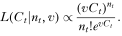
The most likely value of Ct, denoted Ĉt, is the value of Ct that maximizes this equation. So, taking the derivative of equation 19, setting it to zero and solving for Ct we get

Rearranging gives equation 1. The standard error in Ct, that is, the uncertainty around the expected value Ĉt is given by
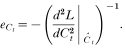
By solving the second derivative of equation 19 and substituting in equation 20 we arrive at equation 3.
The expected values of the frequencies of the two cell-types,

and

, are found in a similar fashion, but now with the likelihood proportional to equation 16. To find
and efl, fs=1−fl and ns=mt−nl have to be substituted into equation 16. Similarly for
and efs.
The expected slender cell concentration, Ĉl, is given by

. The standard error in Ĉl is given by the relation (Squires, 1985)

This is easily rearranged to give equation 5.
APPENDIX B: NORMALIZING SIF PRODUCTION
We assume that SIF is produced at a rate a11 and degraded at a rate a5, that is

SIF induces L1 differentiation
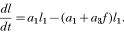
Because we do not have any indication of SIF production rate or its quantitative effect on L1 cells, we can manipulate the equations to subsume parameter a11 into parameter a3 like so.
Let SIF concentration be composed of a constant factor F that represents the units of measurement, and a number f* that has no dimensions i.e., f=Ff*. Substituting this into equations 23 and 24, setting F=a11 and dividing through gives
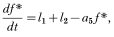
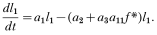
For convenience we write f* as f, and subsume parameter a11 into a3 with no loss of generality.
APPENDIX C: CONVERTING THE DDE MODEL TO AN ODE MODEL
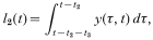
To convert the DDE model into an ODE model we have to have two classes of cells: an uncommitted class and a differentiated class. The former is just L1 of the DDE model. The latter includes classes L2, L3 and S. The concentration of the uncommitted class is just l1, as before. However, cells in the differentiated class must be traced back from when they differentiated. We do this by defining the variable y(τ, t)δτ, which is the concentration of differentiated cells, at time t, that differentiated between the times τ and τ+δτ. Depending on how long in the past a cell differentiated it will be a dividing slender cell, an arrested slender cell, or a stumpy cell. The model is defined as follows
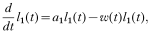


where


null

References
REFERENCES
BARRY, J. D. & TURNER, C. M. R. (1991). The dynamics of antigenic variation and growth of African Trypanosomes. Parasitology Today 7, 207–211.CrossRefGoogle Scholar
BLACK, S. J., HEWETT, R. S. & SENDASHONGA, C. N. (1982). Trypanosoma brucei variable surface antigen is released by degenerating parasites but not by actively dividing parasites. Parasite Immunology 4, 233–244.CrossRefGoogle Scholar
BLACK, S. J., SENDASHONGA, C. N., O'BRIAN, C., BOROWY, N. K., NAESSENS, M., WEBSTER, P. & MURRAY, M. (1985). Regulation of parasitemia in mice infected with Trypanosoma brucei. Current Topics in Microbiology and Immunology 117, 93–118.Google Scholar
HESSE, F., SELZER, P. M., MÜHLSTÄDT, K. & DUSZENKO, M. (1995). A novel cultivation technique for long-term maintenance of bloodstream form trypanosomes in vitro. Molecular and Biochemical Parasitology 70, 157–166.CrossRefGoogle Scholar
PRESS, W. H., TEUKOLSKY, S. A., VETTERLING, W. T. & FLANNERY, B. P. (1992). Numerical Recipies in C: The Art of Scientific Computing, 2nd Edn. Cambridge University Press, Cambridge.
REUNER, B., VASSELLA, E., YUTZY, B. & BOSHART, M. (1997). Cell density triggers to stumpy differentiation of Trypanosoma brucei bloodstream forms in culture. Molecular and Biochemical Parasitology 90, 269–280.CrossRefGoogle Scholar
SEED, J. R. & BLACK, S. J. (1997). A proposed density-dependent model of long slender to short stumpy transformation in the African trypanosomes. Journal of Parasitology 83, 656–662.CrossRefGoogle Scholar
SEED, J. R. & BLACK, S. J. (1999). A revised arithmetic model of long slender to short stumpy transformation in the African trypanosomes. Journal of Parasitology 85, 850–854.CrossRefGoogle Scholar
SEED, J. R. & SECHELSKI, J. B. (1988). Growth of pleomorphic Trypanosoma brucei rhodesiense in irradiated inbred mice. Journal of Parasitology 74, 781–789.CrossRefGoogle Scholar
SEED, J. R. & SECHELSKI, J. B. (1989 a). African trypanosomes: Inheritance of factors in resistance to the African trypanosomes. Experimental Parasitology 69, 1–8.Google Scholar
SEED, J. R. & SECHELSKI, J. B. (1989 b). Mechanism of long slender (LS) to short stumpy (SS) transformation in the African trypanosomes. Journal of Protozoology 36, 572–577.Google Scholar
SQUIRES, G. L. (1985). Practical Physics, 3rd Edn. Cambridge University Press, Cambridge.
TURNER, C. M. R., ASLAM, N. & DYE, C. (1995). Replication, differentiation, growth and the virulence of Trypanosoma brucei infections. Parasitology 111, 289–300.CrossRefGoogle Scholar
TYLER, K. M., HIGGS, P. G., MATTHEWS, K. R. & GULL, K. (2001). Limitation of Trypanosoma brucei parasitemia results from density-dependent parasite differentiation and parasite killing by the host immune response. Proceedings of the Royal Society London, B 268, 2235–2243.CrossRefGoogle Scholar
TYLER, K. M., MATTHEWS, K. R. & GULL, K. (1997). The bloodstream differentiation-division of Trypanosoma brucei studied using mitochondrial markers. Proceedings of the Royal Society London, B 264, 1481–1490.CrossRefGoogle Scholar
VASSELLA, E., REUNER, B., YUTZY, B. & BOSHART, M. (1997). Differentiation of African trypanosomes is controlled by a density sensing mechanism which signals cell cycle arrest via the cAMP pathway. Journal of Cell Science 110, 2661–2671.Google Scholar
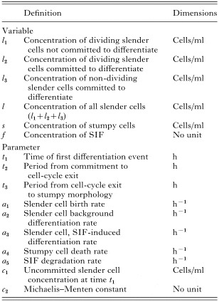
Table 1. Model variables and parameters
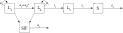
Fig. 1. Schematic representation of the model. Slender cells, denoted L, are split into 3 subclasses: those not committed to differentiate, denoted L1, those committed to differentiate but still dividing, denoted L2, and those committed to differentiate and not dividing, denoted L3. Stumpy cells are denoted S. The parameters are defined in Table 1 and the model details are given in the text.

Fig. 2. Solid lines: (A) Michaelis–Menten kinetics of slender cell differentiation rate. (B) As SIF concentration is increasing exponentially, Michaelis–Menten kinetics gives switch like behaviour in the differentiation rate. The dotted lines represent differentiation rate proportional to SIF concentration i.e., a3f. For an exponentially increasing population, such a rate also gives switch-like behaviour.
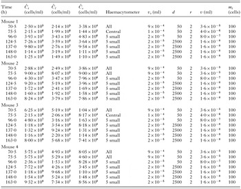
Table 2. Given cell concentrations and experimental parameters
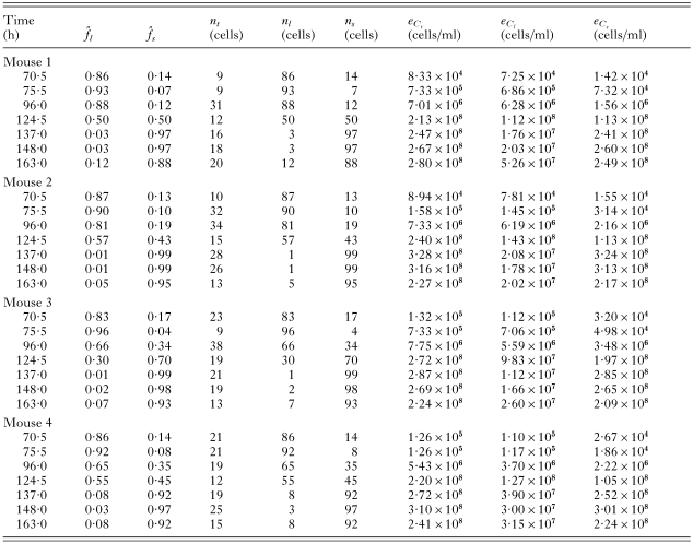
Table 3. Reconstructed raw data
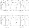
Fig. 3. Experimental results (circles) with error bars (±1 S.E.M.). One error bar extends to zero. The x-axis gives the time since the start of the experiment, and the y-axis the number of cells/ml on a log scale.
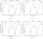
Fig. 4. Best-fit curves. Circles are observed values, lines are best fits. The x-axis shows time since beginning of experiment, the y-axis shows cell concentration in cells/ml on a log scale. Dotted lines for mouse 3 shows best-fit where cell type concentrations at 75·5 h have been omitted from the fit. Dotted lines for mouse 4 shows best-fit where total and cell type concentrations at 75·5 h have been omitted from the fit.
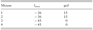
Table 4. The maximum-likelihoods and goodness-of-fits for each mouse
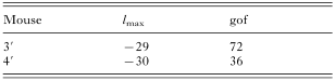
Table 5. The maximum-likelihoods and goodness-of-fits for mouse 3′ and 4′
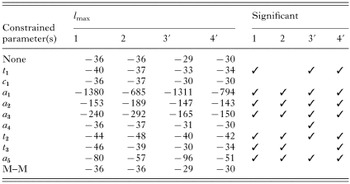
Table 6. Parameter significance
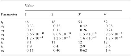
Table 7. Estimated parameter values for best-fit model
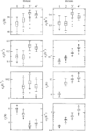
Fig. 5. Boxplots of the estimated parameter distributions. The horizontal line is the median, the box bounds 50% of the values. Circles show outliers.

Fig. 6. Instantaneous differentiation rate from L1 to L2 class (a2+a3f(t)). Solid line: mouse 1; dotted line: mouse 2; dashed line: mouse 3′; dot-dashed line: mouse 4′.

Fig. 7. Extrapolation of the best-fit model for mouse 3 (solid line) shows stable oscillations. Increasing the L2 to L3 transition time by 40% causes the oscillations to decay (dotted line).
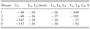
Table 8. Maximum-likelihoods for different combinations of cells producing SIF

Fig. 8. If stumpy cells produce SIF then too much is produced and the slender cell concentration drops too low (dashed line). If only uncommitted cells produce SIF then too little is produced and the slender cell concentration does not drop far enough (dotted line). The best-fit model for mouse 1 was used.
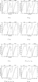
Fig. 9. Effect of changing the parameter values for the best fit model of mouse 2. (A) Dotted: a1×1·2, dashed: a1/2. (B) Dotted: a2×2, dashed: a2=0. (C) Dotted: a3×500, dashed: a3/5. (D) Dotted: a4=0·7, dashed: a4=0. (E) Dotted: t2×2, dashed: t2=0. (F) Dotted: t3×10, dashed: t3=0, L1 and L2 produce SIF. (G) Dotted: t3×10, dashed: t3=0, L1, L2 and L3 produce SIF. (H) Dotted: a5×2, dashed: a5=0.
 You have
Access
- 14
- Cited by