



1. Introduction
Buoyancy-driven bubbly flows are ubiquitous in both natural and industrial environments, ranging from breaking waves and hydrothermal vents to bubble columns and metallurgical reactors. Understanding the rise dynamics of individual bubbles and their mutual interactions remains a central problem for elucidating the fundamental mechanisms governing momentum, mass and heat transfer in freely rising suspensions (Maeda et al. Reference Maeda, Date, Sugiyama, Takagi and Matsumoto2021; Legendre & Zenit Reference Legendre and Zenit2025). Among the many configurations observed in bubble swarms, the rise of an in-line bubble pair provides the simplest yet most informative prototype of hydrodynamic interaction. It encapsulates the essential coupling mechanisms, e.g. wake entrainment, drag reduction and lift generation, that govern the collective dynamics of larger bubble populations (Zenit, Koch & Sangani Reference Zenit, Koch and Sangani2001; Figueroa-Espinoza et al. Reference Figueroa-Espinoza, Mena, Aguilar-Corona and Zenit2018; Ma et al. Reference Ma, Hessenkemper, Lucas and Bragg2023; Hessenkemper et al. Reference Hessenkemper, Bragg, Lucas and Ma2025). Whether the in-line configuration remains stable or evolves towards an oblique arrangement determines the emergence of vertical chains or horizontal clusters in bubble swarms, making its stability a cornerstone for understanding self-organization in dispersed bubbly flows.
Schematic representations of different interaction scenarios for a pair of rising bubbles.
 $(a)$
Initial configuration of two in-line spherical bubbles;
 $(b)$
stable in-line configuration leading to bubble coalescence;
 $(c)$
unstable drafting–kissing–tumbling (DKT) scenario;
 $(d)$
unstable asymmetric side escape (ASE) scenario.

The in-line configuration was first examined under the assumption of spherical bubbles, as sketched in figure 1
 $(a)$
. In weakly inertial regimes corresponding to low Reynolds numbers, Katz & Meneveau (Reference Katz and Meneveau1996) observed that the two bubbles invariably collide and coalesce, a result confirmed experimentally in silicone oils by Watanabe & Sanada (Reference Watanabe and Sanada2006). This behaviour stems from the viscous attraction produced by the wake region behind the leading bubble (LB), which tends to stabilize the in-line arrangement, as shown in figure 1(b). At moderate Reynolds numbers, however, Hallez & Legendre (Reference Hallez and Legendre2011) numerically demonstrated that the in-line configuration becomes unstable, in agreement with earlier theoretical predictions (Harper Reference Harper1970; Yuan & Prosperetti Reference Yuan and Prosperetti1994). Under these conditions, the trailing bubble (TB) drifts laterally away from the symmetry axis. Depending on the response of the LB to this lateral deviation, two distinct unstable evolutions may occur: the well-known DKT sequence (see figure 1
c), in which both bubbles depart from their initial trajectory, and the ASE scenario (see figure 1
d), in which the LB remains nearly unperturbed while the TB migrates laterally. These two instability scenarios have markedly different consequences for the spatial dispersion of bubbles in a plume. Both scenarios originate from the destabilizing lift acting on the TB, which results from the combined effects of the repulsive potential interaction and the shear induced by the asymmetric wake of the LB. They differ, however, in the strength of the feedback exerted by the escaping TB on the LB. When the lateral motion of the TB substantially distorts the interbubble flow and induces a significant transverse response of the LB, the pair undergoes a DKT-type evolution. When this feedback remains weak, the LB continues to rise almost vertically and the instability takes the form of an ASE event. As the bubbles become deformable and adopt oblate shapes, the interaction dynamics change markedly. Although both the DKT and ASE scenarios persist in experiments (Kusuno & Sanada Reference Kusuno and Sanada2015; Kusuno, Yamamoto & Sanada Reference Kusuno, Yamamoto and Sanada2019) and direct numerical simulations (DNS) (Bunner & Tryggvason Reference Bunner and Tryggvason2003; Gumulya et al. Reference Gumulya, Utikar, Evans, Joshi and Pareek2017; Zhang, Ni & Magnaudet Reference Zhang, Ni and Magnaudet2021), a reversal of the stability trend is observed once the bubbles become sufficiently oblate, corresponding to a restabilized in-line configuration that may even lead to head-on collision. Recent three-dimensional Lagrangian tracking experiments by Hessenkemper et al. (Reference Hessenkemper, Bragg, Lucas and Ma2025) further showed that smaller, nearly spherical bubbles in plumes exhibit random pair alignments, confirming that less deformed bubbles are more sensitive to flow perturbations.
This brief review highlights that determining how the bubble aspect ratio influences the stability of the in-line configuration is of essential importance. To date, the prevailing interpretation attributes the restabilization observed for oblate bubbles to the enhanced viscous entrainment in the LB’s wake, which draws the TB back towards the symmetry axis and offsets the destabilizing lift. Since neither the potential nor the shear-induced components of the lift can change sign within the investigated parameter range, this explanation has remained quite qualitative. The persistence of this ambiguity provides the main motivation for the present study, which aims to address two fundamental questions: (a) Is the observed stabilization of oblate bubble pairs genuinely caused by deformation-enhanced wake entrainment, or does it originate from a different physical mechanism? (b) Do the DKT and ASE evolutions represent two manifestations of a single instability, or do they correspond to distinct global modes of the coupled bubble–flow system?
The present work revisits this problem through a global linear stability analysis (LSA) formulated within an arbitrary Lagrangian–Eulerian (ALE) framework. This formulation is essential because conventional LSAs, defined on fixed computational domains, cannot properly account for the evolving geometry arising from the relative motion of two bubbles. Classical LSAs have proved powerful for elucidating the onset of wake and path instabilities in isolated bodies. For fixed spheroids or disks, global analyses have established that the first loss of axisymmetry originates within the recirculation zone of the wake (Meliga, Chomaz & Sipp Reference Meliga, Chomaz and Sipp2009; Tchoufag, Magnaudet & Fabre Reference Tchoufag, Magnaudet and Fabre2013; Cano-Lozano et al. Reference Cano-Lozano, Tchoufag, Magnaudet and Martínez-Bazán2016). When the body is allowed to move freely under buoyant forcing, the coupling between hydrodynamic and kinematic degrees of freedom gives rise to oscillatory modes responsible for the zigzag or spiral trajectories of rising bubbles (Tchoufag et al. Reference Tchoufag, Magnaudet and Fabre2014b ; Cano-Lozano et al. Reference Cano-Lozano, Tchoufag, Magnaudet and Martínez-Bazán2016) and disks (Assemat, Fabre & Magnaudet Reference Assemat, Fabre and Magnaudet2012; Tchoufag et al. Reference Tchoufag, Fabre and Magnaudet2014a ). In the present ALE–LSA approach, the time-dependent configuration is mapped onto a steady reference domain, allowing the linearized Navier–Stokes equations to be solved for the global eigenmodes of the coupled bubble–flow system. This methodology, previously applied to deformable single bodies (Pfister & Marquet Reference Pfister and Marquet2020; Bonnefis et al. Reference Bonnefis, Sierra-Ausin, Fabre and Magnaudet2024), captures both the translational and rotational degrees of freedom of each bubble, thereby resolving the full structure of the two-way hydrodynamic coupling.
The results reveal that the stabilization of oblate bubble pairs does not originate from a deformation-dependent reversal of wake entrainment, as previously assumed, but instead from an inclination-induced rotational feedback. A small lateral disturbance generates a shear-induced torque on the TB that reorients its minor axis towards the outward side of the wake. As the rotation proceeds, an opposing inertial torque develops, and the two balance at a finite inclination angle where the bubble’s broadside faces the local shear. This orientation modifies the surface-pressure distribution, producing a restoring lift directed towards the symmetry axis and thereby counteracting the destabilizing potential and shear-induced components of the lift. The present analysis also clarifies the dynamical distinction between the DKT and ASE evolutions, which are shown to correspond to different global response modes of the coupled bubble–flow system. In the DKT regime, the hydrodynamic interaction between the two bubbles is strongly reciprocal: the self-rotation of each bubble plays a significant role, and their motions remain dynamically coupled throughout the instability growth. By contrast, the ASE regime behaves more like a one-way coupling problem, where the LB primarily imposes a shear environment, and the stability characteristics are governed almost entirely by the response of the TB. In addition, the analysis uncovers a previously unreported oscillatory global mode, which does not result from periodic vortex shedding as in isolated bubbles, but from the unsteady recirculation connecting the two bubbles. This confined vortical structure acts as a hydrodynamic spring that links their motions and mediates a phase-lagged exchange of momentum and torque. By combining the ALE–LSA framework with fully resolved embedded boundary method (EBM) simulations, we isolate and quantify these mechanisms over a broad range of Reynolds numbers and aspect ratios. The resulting physical picture revises the classical interpretation of lift reversal and establishes a unified framework for predicting stability transitions in interacting bubble pairs – and, by extension, in more complex bubbly flows.
The paper is organized as follows. Section 2 introduces the problem formulation, the governing dimensionless parameters, and the numerical implementation of the global ALE–LSA framework. Section 3 describes the steady axisymmetric base flows and examines their dependence on bubble shape, separation distance and Reynolds number, with particular emphasis on the equilibrium distance and the formation of the standing eddy connecting the two bubbles. Section 4 presents the stability characteristics of the stationary mode obtained from the ALE–LSA. Special attention is devoted to three aspects governing this mode: the influence of bubble rotation, the role of mutual hydrodynamic coupling in the DKT and ASE regimes, and the effect of a realistic deformation contrast between the leading and TBs. The EBM (Zhang et al. Reference Zhang, Wei, Meng and Ni2025; Wei, Zhang & Ni Reference Wei, Zhang and Ni2026) is further employed to compute the lift and torque acting on fixed in-line bubbles, providing quantitative support for the key role of bubble inclination in controlling the stability of the in-line configuration. Section 5 then examines the oscillatory global mode, which originates from the unsteady hydrodynamic coupling mediated by the interbubble recirculation. Finally, the main findings and concluding remarks are summarized in § 6.
2. Problem statement and linear stability strategy
2.1. Problem description
The steady, axisymmetric base configuration of the in-line bubble pair is sketched in figure 2
 $(a)$
, where the main geometric parameters are defined. The problem is described in a Cartesian frame
 $(X,Y,Z)$
, or equivalently in cylindrical coordinates
 $(x,r,\theta )$
, with
 $x$
denoting the vertical direction. Two identical gas bubbles, hereafter referred to as the LB and TB, rise in line with a common dimensional velocity
 $-V_x\boldsymbol{e}_x$
through an incompressible Newtonian liquid of density
 $\rho \,(\mathrm{kg\,m^{-3}})$
and dynamic viscosity
 $\mu \,(\mathrm{kg\,m^{-1}\,s^{-1}})$
. In the frame translating with the bubble pair, the surrounding liquid therefore approaches the bubbles with velocity
 $V_x\boldsymbol{e}_x$
, where
 $V_x$
is measured in metres per second. Each bubble is modelled as a non-deformable spheroid of fixed volume, characterized by the aspect ratio
 $\chi =b/a$
, where
 $a$
and
 $b$
are the dimensional minor and major semiaxes, respectively. The equivalent spherical radius is defined as
 $R=(b^2a)^{1/3}$
, with
 $R$
measured in metres. The Reynolds number is based on the equivalent diameter
 $2R$
and the common rise velocity
 $V_x$
, namely
 $ \textit{Re}=2\rho V_xR/\mu$
. Since both bubbles rise with the same velocity in the base state, their dimensional centre-to-centre distance remains constant and is denoted by
 $\bar {S}$
. The corresponding dimensionless separation is
 $S=\bar {S}/(2R)$
. The dimensionless surface-to-surface gap is then
 $\delta S=S-\chi ^{-2/3}$
, which represents the minimum axial distance between the two interfaces normalized by
 $2R$
. Bubble contact corresponds to
 $\delta S=0$
, i.e.
 $S=\chi ^{-2/3}$
; this gives
 $S=1$
for spherical bubbles (
 $\chi =1$
) and
 $S\simeq 0.63$
for oblate bubbles with
 $\chi =2$
. Thus,
 $\rho$
,
 $\mu$
,
 $V_x$
,
 $a$
,
 $b$
,
 $R$
and
 $\bar {S}$
are dimensional quantities, whereas
 $ \textit{Re}$
,
 $\chi$
,
 $S$
and
 $\delta S$
are dimensionless parameters. The dimensional geometric parameters are illustrated in the
 $(x,r)$
meridional plane in figure 2
 $(c)$
, and the corresponding ALE–LSA formulation is detailed in § 2.3.
Considering that the density and viscosity of the gas enclosed in the bubble are negligibly small compared with those of the surrounding liquid, the base flow is thus fully characterized by the dimensionless parameters
 $( \textit{Re},\,\chi ,\,S)$
, or equivalently
 $( \textit{Re},\,\chi ,\,\delta S)$
. In real gas–liquid systems these parameters are not strictly independent, as they jointly depend on the fluid properties, bubble size and release intervals. Varying them independently, as done here, should therefore be viewed as a parametric continuation that isolates the respective influences of inertia, shape and bubble–bubble interaction, even though such decoupling cannot be achieved experimentally. Throughout this study, the aspect ratio is restricted to
 $\chi \leqslant 1.9$
, a range over which the wake of the bubbles pair remains steady and axisymmetric, and this restriction ensures that any departure from the in-line configuration results exclusively from hydrodynamic interaction between the two bubbles rather than from intrinsic wake unsteadiness. This assumption is explicitly confirmed in Appendix C, and will also be discussed in § 4.
Sketch of the bubble-pair configuration (detailed descriptions are provided in the main text).
 $(a)$
Steady, axisymmetric base flow and definition of the principal geometric parameters.
 $(b)$
Typical unstable configurations following an infinitesimally imposed lateral perturbation.
 $(c)$
Computational domain and spatial discretization adopted for the ALE–LSA simulations.

Figure 2
 $(b)$
illustrates the reference configuration adopted to describe small deviations from perfect in-line alignment. In the absolute (laboratory) frame, the instantaneous positions and velocities of the leading and TBs are denoted by
 $\boldsymbol{X}_{\textit{LB}} = (X,\,Y,\,Z)_{\textit{LB}}$
,
 $\boldsymbol{X}_{\textit{TB}} = (X,\,Y,\,Z)_{\textit{TB}}$
and
 $\boldsymbol{V}_{\textit{LB}} = (-V_x,\,V_y,\,V_z)_{\textit{LB}}$
,
 $\boldsymbol{V}_{\textit{TB}} = (-V_x,\,V_y,\,V_z)_{\textit{TB}}$
, respectively. For the computations, we introduce a second Cartesian frame
 $(x, y, z)$
translating with the LB, whose
 $x$
-axis remains aligned with the vertical direction while the
 $y$
–
 $z$
plane defines the transverse plane. In this moving frame, the dimensional positions of the bubble centres are
 $\boldsymbol{\widetilde {X}}_{\textit{LB}} = (0,\,0,\,0)$
and
 $\boldsymbol{\widetilde {X}}_{\textit{TB}} = (\bar {S},\,Y_{\textit{TB}}-Y_{\textit{LB}},\,Z_{\textit{TB}}-Z_{\textit{LB}})$
. This coordinate system conveniently accounts for the relative displacement between the two bubbles and forms the reference framework for the subsequent stability analysis. A lateral displacement of the TB defines an instantaneous inclination angle
 $\varPsi = \tan ^{-1}\! (\sqrt {(Y_{\textit{TB}} - Y_{\textit{LB}})^2 + (Z_{\textit{TB}} - Z_{\textit{LB}})^2}/\bar {S} )$
, which quantifies the deviation of the line joining the bubble centres from the vertical. Unlike in studies of isolated bubbles (Tchoufag et al. Reference Tchoufag, Magnaudet and Fabre2014b
; Cano-Lozano et al. Reference Cano-Lozano, Tchoufag, Magnaudet and Martínez-Bazán2016), the present coordinate system does not rotate with the LB, as the relative motion of the TB renders such a frame unsuitable for describing their coupled dynamics.
To describe the orientation of each bubble, we introduce the Euler angles, more precisely the Tait–Bryan angles, denoted by
 $\boldsymbol{\varXi }_{(\textit{LB},\textit{TB})}=[\alpha ,\,\beta ,\,\gamma ]^T_{(\textit{LB},\textit{TB})}$
. We adopt the extrinsic
 $\textit{XYZ}$
convention, so that
 $\alpha$
,
 $\beta$
and
 $\gamma$
correspond to successive rotations about the fixed
 $x$
,
 $y$
and
 $z$
axes of the inertial frame. The angular velocity
 $\boldsymbol{\varOmega }_{(\textit{LB},\textit{TB})}$
is therefore not, in general, equal to
 ${\rm d}\boldsymbol{\varXi }_{(\textit{LB},\textit{TB})}/{\rm d}t$
, but is related to the Euler-angle rates through a nonlinear kinematic transformation, given below in (2.2d
). However, since the stability analysis only involves infinitesimal perturbations about the axisymmetric base state, this relation reduces at leading order to
 $\boldsymbol{\varOmega }_{(\textit{LB},\textit{TB})}=[\dot {\alpha },\,\dot {\beta },\,\dot {\gamma }]^T_{(\textit{LB},\textit{TB})}+O(|\boldsymbol{\varXi }|\,|\dot {\boldsymbol{\varXi }}|)$
, where
 $(\dot {\,})$
denotes
 ${\rm d}/{\rm d}t$
. Moreover, the rotation about the symmetry axis of an axisymmetric spheroid does not contribute to the hydrodynamic force or torque associated with the lateral path-instability modes. We therefore retain only the two transverse angular degrees of freedom and introduce the reduced orientation vector
 $\boldsymbol{\varTheta }_{(\textit{LB},\textit{TB})}=[0,\,\beta ,\,\gamma ]^T_{(\textit{LB},\textit{TB})}$
, together with
 $\boldsymbol{\varOmega }_{(\textit{LB},\textit{TB})}=[0,\,\dot {\beta },\,\dot {\gamma }]^T_{(\textit{LB},\textit{TB})}$
at the linear order. Hence,
 $\varPsi$
characterizes the revolution of the TB about the LB, while
 $\boldsymbol{\varXi }$
(or
 $\boldsymbol{\varTheta}$
) quantifies its intrinsic rotation. When infinitesimal perturbations are superimposed on the steady base state, growth of
 $\varPsi$
indicates an unstable in-line configuration, whereas the remaining zero value corresponds to a stable alignment. These kinematic quantities are used consistently hereafter to describe both the steady base flow and its linear perturbations.
Note that the present configuration departs from realistic bubble pairs in two respects. First, experiments (Sanada, Watanabe & Fukano Reference Sanada, Watanabe and Fukano2006; Maeda et al. Reference Maeda, Date, Sugiyama, Takagi and Matsumoto2021) and three-dimensional volume of fluid–DNS (VOF–DNS) studies (Gumulya et al. Reference Gumulya, Utikar, Evans, Joshi and Pareek2017; Zhang et al. Reference Zhang, Ni and Magnaudet2021) have shown that the TB generally exhibits a smaller aspect ratio than the LB, since the low-pressure region in the wake of the latter tends to make the TB more spherical. For clarity and tractability, both bubbles are here prescribed identical spheroidal shapes (
 $\chi _{\textit{LB}}=\chi _{\textit{TB}}=\chi$
), allowing the fundamental mechanisms destabilizing the in-line configuration to be isolated. The influence of unequal aspect ratios is examined separately in § 4.5. Second, under realistic conditions the TB typically accelerates slightly faster than the LB before reaching equilibrium separation (Sanada et al. Reference Sanada, Watanabe and Fukano2006; Gumulya et al. Reference Gumulya, Utikar, Evans, Joshi and Pareek2017; Zhang et al. Reference Zhang, Ni and Magnaudet2021), so that
 $V_{x,TB} \gt V_{x,LB}$
in practice. For simplicity, both bubbles are here assumed to rise at the same mean velocity, so that the analysis focuses on the intrinsic stability of the steady in-line configuration. This approximation, which has limited influence on the instability mechanism, is consistent with previous numerical studies of bubble–bubble interactions (Legendre, Magnaudet & Mougin Reference Legendre, Magnaudet and Mougin2003; Hallez & Legendre Reference Hallez and Legendre2011).
2.2. Governing equations and ALE formulation
Because the gas density and viscosity are negligible compared with those of the surrounding liquid, the internal motion within each bubble may be ignored and the gas pressure treated as spatially uniform (Magnaudet & Mougin Reference Magnaudet and Mougin2007; Tchoufag et al. Reference Tchoufag, Magnaudet and Fabre2013, Reference Tchoufag, Magnaudet and Fabre2014b
; Bonnefis et al. Reference Bonnefis, Sierra-Ausin, Fabre and Magnaudet2024). Accordingly, the dynamics of the system are entirely governed by the liquid motion in the external domain
 $\varUpsilon (t)$
, coupled with the translational and rotational motions of the two bubbles. As introduced earlier, the absolute velocity field is projected onto a reference frame translating with the LB, and in this frame, the incompressible liquid flow satisfies the mass and momentum equations
 \begin{align} \boldsymbol{\nabla } \boldsymbol{\cdot } \boldsymbol{u} &= 0, \qquad \qquad \quad \text{in } \quad \varUpsilon (t), \\[-12pt]\nonumber \end{align}
 \begin{align} \rho \!\left ( \frac {\partial \boldsymbol{u}}{\partial t} + (\boldsymbol{u} - \boldsymbol{V}_{\textit{LB}}) \boldsymbol{\cdot } \boldsymbol{\nabla }\boldsymbol{u} \right ) &= \boldsymbol{\nabla } \boldsymbol{\cdot } \boldsymbol{\varSigma } (\boldsymbol{u}, p), \quad \text{in } \quad \varUpsilon (t), \end{align}
where
 $\boldsymbol{u}$
and
 $p$
denote the liquid velocity and pressure, respectively. The Newtonian stress tensor is
 $\boldsymbol{\varSigma } (\boldsymbol{u}, p) = -p\,\mathbb{I} + \mu \,(\boldsymbol{\nabla }\boldsymbol{u} + \boldsymbol{\nabla }\boldsymbol{u}^{T})$
, with
 $\mathbb{I}$
the identity tensor, and
 $\boldsymbol{V}_{\textit{LB}}$
is the translational velocity of the LB in the Lagrangian framework.
The motion of each bubble obeys Newton’s laws, which express the balance of hydrodynamic forces and torques acting on its surface
 $\mathscr{S}_{(\textit{LB},\textit{TB})}(t)$
,
 \begin{align} {\rm d}(M\boldsymbol{V})/{\rm d}t &= (M - \rho \mathscr{V}\,)\,\boldsymbol{g} + \int _{\mathscr{S}\,(t)} \boldsymbol{\varSigma } \boldsymbol{\cdot }\boldsymbol{n}\,{\rm d}S, \\[-12pt]\nonumber \end{align}
 \begin{align} {\rm d}\left (\mathbb{J} \boldsymbol{\cdot }\boldsymbol{\varOmega }\right )/{\rm d}t&= \int _{\mathscr{S}\,(t)} \boldsymbol{r}\!\times \!(\boldsymbol{\varSigma } \boldsymbol{\cdot }\boldsymbol{n})\,{\rm d}S, \\[-12pt]\nonumber \end{align}
 \begin{align} {\rm d}\boldsymbol{X}/{\rm d}t &= \boldsymbol{V}, \\[-12pt]\nonumber \end{align}
 \begin{align} \boldsymbol{\varOmega } = \begin{bmatrix} \varOmega _x \\[3pt] \varOmega _y \\[3pt] \varOmega _z \end{bmatrix} &= \begin{bmatrix} \cos \gamma \cos \beta & -\sin \gamma & 0 \\[3pt] \sin \gamma \cos \beta & \cos \gamma & 0 \\[3pt] -\sin \beta & 0 & 1 \end{bmatrix} \begin{bmatrix} \dot {\alpha } \\[3pt] \dot {\beta } \\[3pt] \dot {\gamma } \end{bmatrix}\!, \end{align}
where subscripts for the LB and TB are omitted for brevity, and
 $\int _{\mathscr{S}\,(t)}$
indicates the hydrodynamic forces and torques are computed directly by integrating the fluid stress, or its ALE counterpart, the first Piola–Kirchhoff stress tensor, over the bubble surface. Here,
 $\boldsymbol{X}$
and
 $\boldsymbol{\varXi } = (\alpha , \beta , \gamma )$
denote the translational displacement and the angular displacement of the bubble, respectively. Here
 $\boldsymbol{V}$
and
 $\boldsymbol{\varOmega }$
are the corresponding translational and angular velocities, and
 $\boldsymbol{r}$
is the position vector relative to the centre. The unit normal to the interface
 $\mathscr{S}$
is denoted by
 $\boldsymbol{n}$
. Each bubble has a volume
 $\mathscr{V} = ({4}/{3})\pi a b^{2}$
, mass
 $M = \rho _b\mathscr{V}$
. In the axisymmetric base state, the bubbles do not rotate and their symmetry axes are aligned with the streamwise direction. The inertia tensor is then diagonal in the inertial frame and is given by
 $\mathbb{J}_0=J_{1}\boldsymbol{xx}+J_{2}(\boldsymbol{yy}+\boldsymbol{zz})$
, with
 $J_{1}=({2}/{5})Mb^{2}$
and
 $J_{2}=({1}/{5})M(a^{2}+b^{2})$
. For a finite rotation, however, the inertia tensor entering (2.2b
) must be expressed in the inertial frame as
 $\mathbb{J}=\mathbb{R}\mathbb{J}_0\mathbb{R}^{T}$
, where
 $\mathbb{R}$
is the rotation matrix associated with the instantaneous orientation of the bubble. With the convention adopted in (2.2d
), this matrix reads
 \begin{align} \mathbb{R}=\mathbb{R}_z(\gamma )\mathbb{R}_y(\beta )\mathbb{R}_x(\alpha ) = \begin{bmatrix} c_\beta c_\gamma & s_\alpha s_\beta c_\gamma -c_\alpha s_\gamma & c_\alpha s_\beta c_\gamma +s_\alpha s_\gamma \\[3pt] c_\beta s_\gamma & s_\alpha s_\beta s_\gamma +c_\alpha c_\gamma & c_\alpha s_\beta s_\gamma -s_\alpha c_\gamma \\[3pt] -s_\beta & s_\alpha c_\beta & c_\alpha c_\beta \end{bmatrix}\!, \end{align}
where
 $s_\alpha =\sin \alpha$
,
 $c_\alpha =\cos \alpha$
, and analogous notations are used for
 $\beta$
and
 $\gamma$
. Equations (2.2d
) and the above expression for
 $\mathbb{R}$
provide the nonlinear relation between the angular coordinates and the angular velocity. In the present LSA, only infinitesimal rotations about the axisymmetric base state are retained. Hence,
 $\boldsymbol{\varOmega }=[\dot {\alpha },\,\dot {\beta },\,\dot {\gamma }]^T+O(|\boldsymbol{\varXi }|\,|\dot {\boldsymbol{\varXi }}|)$
and
 $\mathbb{R}=\mathbb{I}+O(|\boldsymbol{\varXi }|)$
. Consequently, the variations of
 $\mathbb{J}$
only contribute to
 ${\rm d}(\mathbb{J}\boldsymbol{\varOmega })/{\rm d}t$
at second order, and the angular-momentum equation reduces, at the linear order, to
 $\mathbb{J}_0\boldsymbol{\cdot }{\rm d}\boldsymbol{\varOmega }/{\rm d}t$
balanced by the linearized hydrodynamic torque. Since the density of the gas is much smaller than that of the ambient fluid (
 $\rho _b \ll \rho$
), its mass
 $M$
and inertia tensor
 $\mathbb{J}$
are negligible and can be assumed to approach zero in the governing equations.
Because the bubbles do not translate in the
 $x$
-direction, the
 $x$
-component equations of (2.2a
) and (2.2c
) thus vanish. On each bubble surface, the interface is non-penetrable and shear-free, leading to the boundary conditions
 \begin{equation} \boldsymbol{u} \boldsymbol{\cdot }\boldsymbol{n} = (\boldsymbol{V} + \boldsymbol{\varOmega }\!\times \!\boldsymbol{r}) \boldsymbol{\cdot }\boldsymbol{n}, \quad \boldsymbol{n}\!\times \!(\boldsymbol{\varSigma } \boldsymbol{\cdot }\boldsymbol{n}) = \boldsymbol{0}, \quad \text{on } \quad \mathscr{S}\,(t). \end{equation}
At infinity (
 $|\boldsymbol{x}|\!\to \!\infty$
), the velocity field recovers the uniform far-field velocity
 $\boldsymbol{u} = (0, 0, 0)$
. Lengths, velocities, time and stresses are non-dimensionalized with
 $2R$
,
 $V_{x}$
,
 $2R/V_{x}$
and
 $\rho V_{x}^{2}$
, respectively. The bubble mass and moment of inertia are scaled with
 $8\rho R^{3}$
and
 $3\rho R^{5}$
.
To analyse stability in a configuration where the fluid domain evolves with the bubble motion, the governing equations are recast within an ALE framework. This formulation maps the time-dependent domain
 $\varUpsilon (t)$
onto a fixed reference configuration
 $\varUpsilon _{0}$
, allowing all variables to be defined on a stationary computational mesh. The mapping
 $\mathcal{A} : \varUpsilon _{0}\!\times \!\mathbb{R}^{+}\!\to \!\varUpsilon (t)\!\times \!\mathbb{R}^{+}$
is defined as
 \begin{equation} \boldsymbol{x} = \boldsymbol{x}_{0} + \boldsymbol{\xi }_{0}(\boldsymbol{x}_{0},t), \end{equation}
where
 $\boldsymbol{x}_{0}$
denotes the position in the reference domain and
 $\boldsymbol{\xi }_{0}$
the mesh–extension displacement field. This auxiliary field transfers the rigid-body motions of both bubble interfaces (
 $\mathscr{S}_{\textit{LB}}$
and
 $\mathscr{S}_{\textit{TB}}$
) smoothly into the surrounding liquid, ensuring a divergence-free and minimally distorted grid. The displacement field
 $\boldsymbol{\xi }_{0}$
is obtained by solving an elliptic extension problem in
 $\varUpsilon _{0}$
, subject to rigid-body boundary conditions on
 $(\mathscr{S}_{\textit{LB}}\,\cup \,\mathscr{S}_{\textit{TB}})$
and homogeneous conditions at the outer boundaries. This approach, initially developed by Bonnefis (Reference Bonnefis2019) and refined by Sierra-Ausin et al. (Reference Sierra-Ausin, Bonnefis, Tirri, Fabre and Magnaudet2022) and Bonnefis et al. (Reference Bonnefis, Sierra-Ausin, Fabre and Magnaudet2024), provides a geometrically consistent description of translating and rotating bodies within a fixed reference domain. Unlike previous isolated-bubble formulations, the present implementation accounts for the simultaneous rigid-body motions of two spheroids, introducing a non-trivial geometric coupling between the two interfaces.
From the mapping (2.5), the local deformation of the fluid domain is characterized by
 \begin{align} \mathbb{F}_{0} = \mathbb{I} + \boldsymbol{\nabla} _{0}\boldsymbol{\xi }_{0}, \quad J_{0} = \det (\mathbb{F}_{0}), \quad \boldsymbol{\varPhi }_{0} = J_{0}\mathbb{F}_{0}^{-1}, \end{align}
where
 $\mathbb{F}_{0}$
is the deformation gradient,
 $J_{0}$
the Jacobian determinant and
 $\boldsymbol{\varPhi }_{0}$
the metric operator linking the instantaneous and reference configurations. In this framework, the velocity and pressure fields,
 $\boldsymbol{u}_{0}(\boldsymbol{x}_{0},t)$
and
 $p_{0}(\boldsymbol{x}_{0},t)$
, are defined on the fixed reference domain
 $\varUpsilon _{0}$
. The continuity and momentum equations (2.1) then become
 \begin{align} \boldsymbol{\nabla} _{0} \boldsymbol{\cdot }(\boldsymbol{\varPhi }_{0}\boldsymbol{u}_{0}) &= 0, \quad \text{in } \quad \varUpsilon _{0}, \end{align}
 \begin{align} J_{0}\rho _0\frac {\partial \boldsymbol{u}_{0}}{\partial t} + \rho _0(\boldsymbol{\nabla} _{0}\boldsymbol{u}_{0}\boldsymbol{\varPhi }_{0}) \left (\boldsymbol{u}_{0} - \frac {\partial \boldsymbol{\xi }_{0}}{\partial t} - \boldsymbol{V}_{\textit{LB}}\right ) - \boldsymbol{\nabla} _{0} \boldsymbol{\cdot }\mathbb{L}_{0}(\boldsymbol{u}_{0},p_{0},\boldsymbol{\xi }_{0}) &= \boldsymbol{0}, \quad \text{in } \quad \varUpsilon _{0}, \end{align}
where
 $\mathbb{L}_{0}$
denotes the first Piola–Kirchhoff stress tensor, ensuring exact momentum conservation under the domain transformation. The hydrodynamic forces and torques acting on each bubble are obtained by integrating
 $\mathbb{L}_{0}$
over their respective surfaces, while the bubble dynamics remain expressed in the Lagrangian form (2.2a
)–(2.2d
). This coupled ALE formulation provides a conservative and geometrically consistent framework for computing the fluid–bubble interaction within a fixed reference geometry, preserving the geometric conservation law and avoiding mesh distortion. Explicit expressions for the transformation operators, the ALE stress tensor and the weak variational formulation employed in the numerical implementation are provided in Appendix A. This ALE framework forms the foundation for the linearization procedure developed in the next § 2.3.
2.3. Linearized-ALE formulation and numerical method
The objective of this analysis is to assess the stability of the in-line configuration of a rising bubble pair. The reference, or base flow, corresponds to a steady, axisymmetric state in which the liquid moves past both bubbles at velocity
 $V_x\boldsymbol{e}_x$
, maintaining a fixed separation distance
 $S$
and a common aspect ratio
 $\chi$
(see figure 2
c). This steady solution, denoted
 $\boldsymbol{\mathscr{Q}}^f_{0} = [\boldsymbol{U}_{0},P_{0}]$
, satisfies the incompressible Navier–Stokes equations (2.1) together with the boundary conditions (2.4). Since no relative motion exists between the bubbles, the base state is stationary and the ALE mapping reduces to the identity transformation. The base flow is computed numerically as a steady solution of the axisymmetric momentum equations.
To examine the stability of this configuration, infinitesimal three-dimensional perturbations are superimposed on the base state. Such perturbations may induce relative motions between the bubbles, rendering the fluid domain time-dependent. The equations are therefore recast in the ALE framework introduced in § 2.2, allowing the problem to be formulated on a fixed reference domain while accounting for instantaneous displacements of the bubble interfaces. The coupled liquid–bubble system is described by the state vector
 \begin{align} \mathscr{Q} = [\mathscr{Q}^{f}, \mathscr{Q}^{b}] = [\boldsymbol{u},\,p,\,\boldsymbol{\xi },\,\boldsymbol{X}_{k},\,\boldsymbol{\varXi }_{k},\,\boldsymbol{V}_{k},\,\boldsymbol{\varOmega }_{k}], \quad (k = \text{LB, TB}), \end{align}
where
 $(\boldsymbol{u},p,\boldsymbol{\xi })$
are the fluid variables defined on
 $\varUpsilon _{0}$
, and
 $(\boldsymbol{X}_{k},\boldsymbol{\varXi }_{k},\boldsymbol{V}_{k},\boldsymbol{\varOmega }_{k})$
represent the position, orientation, translational velocity and angular velocity of each bubble.
Each variable is decomposed into a steady base state and a small perturbation,
 \begin{align} \mathscr{Q} = \mathscr{Q}_{0} + \epsilon \,\boldsymbol{q}', \quad \boldsymbol{q}' = [\boldsymbol{u},\,p,\,\boldsymbol{\xi },\,\boldsymbol{X}_{k},\,\boldsymbol{\varXi }_{k},\,\boldsymbol{V}_{k},\,\boldsymbol{\varOmega }_{k}]', \end{align}
where
 $\epsilon \ll 1$
and
 $\boldsymbol{q}'$
denotes the infinitesimal perturbation superimposed on the base flow
 $\mathscr{Q}_{0}$
. Substituting this expansion into the ALE governing equations and retaining only first-order terms yields the linearized-ALE system, which couples the fluid motion to the bubble dynamics through the linearized hydrodynamic forces and torques acting on the bubble surfaces. The corresponding weak variational form and explicit expressions of the linearized operators are given in Appendix A, following the formulation of Tchoufag et al. (Reference Tchoufag, Magnaudet and Fabre2014b
) and Bonnefis et al. (Reference Bonnefis, Sierra-Ausin, Fabre and Magnaudet2024).
Because the base flow is steady and axisymmetric, perturbations are expanded in azimuthal Fourier modes,
 \begin{align} \boldsymbol{q}'(r,\theta ,x,t) = \widetilde {\boldsymbol{q}}(r,x)\,e^{im\theta +\lambda t} + \text{c.c.}, \end{align}
where
 $\widetilde {\boldsymbol{q}}(r,x)$
is the complex amplitude,
 $m$
the azimuthal wavenumber, and
 $\lambda = \lambda _{r} + i\lambda _{i}$
the complex eigenvalue. The real part
 $\lambda _{r}$
represents the growth rate and determines exponential growth or decay, while the imaginary part
 $\lambda _{i}$
gives the oscillation frequency and distinguishes stationary (
 $\lambda _{i} = 0$
) from oscillatory (
 $\lambda _{i} \neq 0$
) modes. Instability occurs for
 $\lambda _{r}\gt 0$
, and the leading global mode corresponds to the eigenpair with the largest
 $\lambda _{r}$
. Axisymmetric perturbations correspond to
 $m=0$
and modify only the axial separation between the two bubbles, without breaking the in-line symmetry. They are therefore not associated with lateral escape and are not considered further here. Modes with
 $|m|\geqslant 2$
correspond to higher azimuthal harmonics of the flow field. After integration over the bubble surface, these modes produce no net lateral force or torque on a rigid bubble and are thus dynamically decoupled from its translational and rotational motion. The present analysis therefore focuses on the non-axisymmetric family
 $|m|=1$
, which is the only family directly coupled to lateral displacement and inclination of the bubbles. These modes represent the first departure from perfect alignment and describe helical disturbances whose linear combinations yield planar zigzag trajectories (Tchoufag et al. Reference Tchoufag, Fabre and Magnaudet2014a
; Bonnefis et al. Reference Bonnefis, Sierra-Ausin, Fabre and Magnaudet2024). For each azimuthal mode, the linearized-ALE equations take the generalized eigenvalue form
 \begin{align} \mathbb{A}_{m}\,\widetilde {\boldsymbol{q}} = \lambda \,\mathscr{B}_{m}\,\widetilde {\boldsymbol{q}}, \end{align}
where
 $\widetilde {\boldsymbol{q}} = [\widetilde {\boldsymbol{q}}^{f},\,\widetilde {\boldsymbol{q}}^{b}]$
collects the fluid and bubble degrees of freedom. The dominant eigenpairs
 $(\lambda ,\widetilde {\boldsymbol{q}})$
are computed using an Arnoldi-based iterative solver applied to the discretized variational form. Convergence and validation are discussed in Appendix B.
Both the base-flow and linear stability analyses are performed with the open-source finite-element solver FreeFem++ (Hecht Reference Hecht2012), where the present ALE framework is implemented by ourselves, following the methodology of Bonnefis et al. (Reference Bonnefis, Sierra-Ausin, Fabre and Magnaudet2024). Spatial discretization employs Taylor–Hood
 $(P_{2},P_{1})$
elements for the velocity–pressure pair and quadratic
 $P_{2}$
elements for the mesh-extension field. The steady base state is obtained via Newton iteration, with linear systems solved by the sparse direct solver UMFPACK. The generalized eigenvalue problem arising from the linearized-ALE formulation is solved using a Krylov–Shur projection method available in SLEPc. Since the base flow is axisymmetric, the problem is discretized on the meridional
 $xor$
plane centred on the LB. An unstructured Delaunay–Voronoi mesh, shown in figure 2
 $(c)$
, ensures adequate resolution near the bubble interfaces and in the wake. Besides the axis boundary at
 $\mathscr{S}_{\textit{axi}}\,(r=0)$
, other boundary conditions are prescribed as follows: a uniform inflow
 $V_{x}\boldsymbol{e}_{x}$
at
 $\mathscr{S}_{\textit{in}}\,(x=-l_{1})$
,
 $\boldsymbol{U_0}=V_{x}\boldsymbol{e}_{x},\ \boldsymbol{u}=\boldsymbol{0}$
; a stress-free outlet at
 $\mathscr{S}_{\textit{out}}\,(x=l_{2})$
,
 $\boldsymbol{\varSigma }(\boldsymbol{U_0},P_0)\boldsymbol{\cdot }\boldsymbol{n}=\boldsymbol{0}, \mathbb{L}_{0}(\boldsymbol{u},p,\boldsymbol{\xi })\boldsymbol{\cdot }\boldsymbol{n} = \boldsymbol{0}$
; an inviscid side boundary at
 $\mathscr{S}_{\textit{side}}\,(r=h)$
,
 $U_{0r}=U_{0\theta }=\partial _rU_{0x}=0,\ u_{r}=u_{\theta }=\partial _ru_{x}=0$
. On
 $\mathscr{S}_{\textit{LB}}$
and
 $\mathscr{S}_{\textit{TB}}$
, the shear-free and non-penetration conditions (2.4) are imposed. The whole computational procedure is described in Appendix A.4.
Accurate computation of the base flow and eigenvalues requires fine resolution near the interfaces and within the wake. Using
 $2R$
as characteristic length, the smallest grid spacing is
 $h_{\textit{min}} = 10^{-3}$
in the radial direction, corresponding to approximately
 $N_r \approx 20$
nodes across a viscous layer of thickness
 $5 \textit{Re}^{-1/2}$
. Along the arc of each bubble, the number of surface nodes per diameter satisfies
 $N_{\theta } \approx 10\, \textit{Re}^{1/2}$
, with at least
 $N_{\theta }=200$
for
 $ \textit{Re}\leqslant 400$
. The computational domain extends to
 $l_{1} = 120$
,
 $l_{2} = 120$
and
 $h = 60$
, substantially larger than that in Bonnefis et al. (Reference Bonnefis, Sierra-Ausin, Fabre and Magnaudet2024), ensuring negligible confinement effects. For these settings, the relative variation of the non-axisymmetric eigenvalues (
 $|m|=1$
) upon mesh refinement remains below
 $0.1\,\%$
. Eigenvalues are computed using an Arnoldi-type Krylov subspace method (Krylov–Schur algorithm) combined with a shift-and-invert spectral transformation. A relative residual tolerance of
 $10^{-8}$
is imposed, and the Krylov subspace dimension is automatically adapted during the iterations. Under these settings, the growth rates and frequencies are found to be converged within
 $10^{-4}$
in non-dimensional units.
All computations were performed under conditions consistent with the three-dimensional VOF–DNS provided by Zhang et al. (Reference Zhang, Ni and Magnaudet2021), namely the corresponding isolated bubble remains rising vertically without performing path instability. The present analysis focuses on cases close to the neutral curves characterizing the stability transition, within
 $ \textit{Re} \lt 200$
and
 $\chi \leqslant 1.9$
, ensuring that the base flow remains steady and free from wake unsteadiness. A detailed mesh-independence and validation study is provided in Appendix B, demonstrating that the solver accurately reproduces the neutral stability curves of a freely falling circular disk (Tchoufag et al. Reference Tchoufag, Fabre and Magnaudet2014a
), a freely rising isolated bubble (Tchoufag et al. Reference Tchoufag, Magnaudet and Fabre2014b
) and tandem-cylinder configurations (Tirri et al. Reference Tirri, Nitti, Sierra-Ausin, Giannetti and de Tullio2023), while also in excellent quantitative agreement with the numerical data (Hallez & Legendre Reference Hallez and Legendre2011; Zhang et al. Reference Zhang, Ni and Magnaudet2021) for spherical in-line bubbles.
3. Steady axisymmetric base flow
Before analysing the stability of the in-line configuration, we first characterize the steady, axisymmetric base flow
 $\boldsymbol{\mathscr{Q}}_{0} = [\boldsymbol{U}_{0}(r, x),\, P_{0}(r, x)]$
, which serves as the reference state for the linearized ALE formulation. The structure of this base flow largely determines both the onset and the nature of the unstable stationary and oscillatory modes identified in §§ 4 and 5, respectively. Two aspects are of primary importance in this respect: (a) the dependence of the flow structure on the prescribed parameters
 $( \textit{Re},\chi ,S)$
, especially the vortical topology within the interbubble gap. These steady fields are computed by holding the two bubbles at a fixed separation
 $S$
in the comoving frame; hence they should be regarded as constrained base states for the subsequent stability analysis, rather than, in general, as equilibrium configurations of a freely rising pair. Their purpose is to isolate how inertia, bubble shape and spacing modify the wake structure that governs the instability discussed below. (b) The particular value
 $S = S_e$
at which the two bubbles experience identical drag forces. This condition defines the equilibrium separation of the one-dimensional in-line motion and provides a useful measure of the hydrodynamic coupling between the bubbles.
3.1. Flow structure
The topology of the flow in the interbubble gap plays an important role in the stability of the in-line configuration. In particular, the formation of a steady recirculating eddy in this region profoundly modifies the hydrodynamic coupling between the bubbles and provides the background flow from which the coupling instability emerges. Before turning to the linear analysis, we therefore characterize the structure and parameter dependence of this steady gap flow, which defines the base state of the system. For an isolated spheroidal bubble, Dandy & Leal (Reference Dandy and Leal1986) and Blanco & Magnaudet (Reference Blanco and Magnaudet1995) showed that, beyond a critical oblateness (
 $\chi \gtrsim 1.65$
), a steady standing eddy forms in the wake, marking the appearance of a closed recirculation region. This feature results from a finite-Reynolds-number balance between vorticity production at the shear-free interface and its downstream advection (Magnaudet & Mougin Reference Magnaudet and Mougin2007). In the present in-line configuration, the threshold aspect ratio and Reynolds number for recirculation differ from the isolated case, since the confined gap flow is controlled by both
 $ \textit{Re}$
and the centre-to-centre distance
 $S$
(or equivalently the gap
 $\delta S$
). In what follows, the aspect ratio
 $\chi$
is kept fixed while
 $ \textit{Re}$
and
 $S$
are varied independently, so as to construct a family of steady axisymmetric base flows past the bubble pair. As already stated in § 2.1, these states are not necessarily equilibrium configurations of a freely rising pair: unless
 $S=S_e$
, where
 $S_e$
denotes the equilibrium separation further detailed in § 3.2, the two bubbles experience different axial forces and would therefore approach or separate in a fully unconstrained evolution. They should instead be viewed as constrained base states, obtained by prescribing the relative axial position of the bubbles in the comoving frame. This continuation in
 $S$
provides a global map of the possible gap-flow topologies and allows the role of the interbubble spacing in the instability mechanism to be isolated.
Phase map associated with the formation of a standing eddy connecting the two bubbles for
 $\chi = 1.3$
.
 $(a)$
Critical curve in the
 $(S,Re)$
(or
 $(\delta S,Re)$
) plane marking the onset of a connected recirculation between the two bubbles, open circle denotes the marginal configuration, corresponding to
 $\textit{Re} \simeq 180$
.
 $(b)$
Streamlines illustrating representative flow structures for the cases indicated in
 $(a)$
: A
 $( \textit{Re}, S) = (30, 0.98)$
, B
 $(100, 0.98)$
, C
 $(100, 1.20)$
and D
 $(100, 1.25)$
. The connected eddy appears at points B and C, whereas points A and D correspond to the unidirection flow structure.

For moderately oblate bubbles (
 $\chi = 1.3$
), figure 3
 $(a)$
maps the steady base flow topologies in the
 $( \textit{Re}, S)$
plane, revealing two distinct regimes within the interbubble gap. Streamlines labelled A and D correspond to a monotonic, unidirectional flow without recirculation, whereas those labelled B and C display a continuous toroidal eddy connecting the wakes of the leading and TBs. The existence and axial extent of this recirculating region are identified from the sign of the streamwise velocity
 $u_x$
along the symmetry axis between the two bubbles. A connected standing eddy is detected when
 $u_x$
reverses sign over the entire axial interval separating the rear stagnation point of the LB from the front stagnation point of the TB. Equivalently, the two zero-crossings of
 $u_x$
that delimit the recirculating region coincide with, or lie outside, the two bubble-facing tips. If the reversed-flow interval occupies only part of the gap, the eddy is regarded as disconnected. Clearly, this standing eddy arises solely from hydrodynamic interaction between the two bubbles, since an isolated bubble of the same aspect ratio does not exhibit wake recirculation. The transition between these regimes is identified by tracking the critical combinations of
 $( \textit{Re}, S)$
, or equivalently
 $( \textit{Re}, \delta S)$
, for which the connected recirculation first appears. For each fixed separation, the lower and upper branches of the transition curve
 $ \textit{Re}_{\textit{min}}$
and
 $ \textit{Re}_{\textit{max}}$
are obtained by locating the values of
 $ \textit{Re}$
at which this reversed-flow interval first spans the entire interbubble gap. Below
 $ \textit{Re}_{\textit{min}}$
, viscous diffusion prevents vorticity accumulation, while above
 $ \textit{Re}_{\textit{max}}$
the
 $ \textit{Re}^{-1/2}$
scaling of the interfacial vorticity flux reduces the circulation strength, suppressing the interbubble connection. The open symbol in the figure marks the marginal configuration, which occurs at
 $ \textit{Re} \approx 180$
.
Same as figure 3, but for a more oblate shape with
 $\chi = 1.9$
.
 $(a)$
Critical curve in the
 $(S, Re)$
(or
 $(\delta S,Re)$
) plane marking the onset of a connected recirculation between the two bubbles.
 $(b)$
Streamlines illustrating the corresponding flow structures for the cases indicated: A
 $(Re, S) = (100, 2.0)$
, B
 $(100, 2.5)$
, C
 $(50, 2.5)$
and D
 $(200, 2.5)$
. The connected eddy appears at point A, whereas points B–D correspond to the detached eddy structure.

Figure 4. Long description
Panel A: A line graph plots Reynolds number (Re) on the vertical axis against a parameter S on the horizontal axis. The graph includes a red curve labeled with a parameter value of 1.9 and four points labeled A, B, C, and D. Panel B: Four streamline diagrams labeled A, B, C, and D show the flow structures corresponding to the points marked on the graph. Each diagram depicts the recirculation zones and flow patterns around the bubbles.
For more oblate bubbles (
 $\chi = 1.9$
), figure 4
 $(a)$
reveals a third flow topology in which a detached recirculating region forms between the two bubbles, as indicated by streamlines B, C and D. In addition, the parameter range supporting a connected recirculation widens markedly. The critical separation extends to
 $S \!\simeq \! 2.4$
(or
 $\delta S \!\simeq \! 1.75$
), and the upper limit
 $ \textit{Re}_{\textit{max}}$
shifts to higher values. As described in Magnaudet & Mougin (Reference Magnaudet and Mougin2007), this trend reflects the
 $\chi ^{7/2} \textit{Re}^{-1/2}$
scaling of the surface vorticity flux: as
 $\chi$
increases, enhanced vorticity generation must be balanced by larger
 $ \textit{Re}$
to sustain comparable advection, thereby allowing the standing eddy to persist over a broader parameter range. The flow fields in figure 4
 $(b)$
confirm that, outside this finite
 $( \textit{Re},S)$
window bounded by the critical curves, the interbubble flow reverts to a detached-eddy topology rather than a unidirectional stream. A small upstream recirculation occasionally appears near the nose of the TB, resulting from vorticity convected from the leading-bubble shear layer and temporarily trapped ahead of the TB.
We do not attempt to present the complete set of critical curves for all aspect ratios, as the comparison between
 $\chi = 1.3$
and
 $\chi = 1.9$
already demonstrates that increasing oblateness enhances vorticity production and promotes the formation of a steady standing eddy within the interbubble gap. This connected recirculation, however, is not a passive wake feature: it constitutes a closed conduit for momentum and vorticity exchange between the two bubbles, acting as a hydrodynamic spring that dynamically couples their motions. As will be shown in § 4, this coupling strongly influences the stability of the DKT-type stationary mode, while in § 5 it underpins the oscillatory instability, where the periodic deformation of the gap flow sustains a self-excited lateral oscillation of the TB.
3.2. Equilibrium distance
Having characterized how the prescribed base-flow structure varies with
 $( \textit{Re},\chi ,S)$
, we now turn to the special member of this family corresponding to the equilibrium separation
 $S_e$
, at which the axial hydrodynamic forces acting on the two bubbles are identical. Strictly speaking, the condition of equal axial force is also recovered asymptotically as
 $S\rightarrow \infty$
, since the hydrodynamic interaction then vanishes and each bubble behaves as an isolated one. In this trivial limit, however, the pair is no longer dynamically coupled. Throughout the present study, the term ‘equilibrium separation’ therefore refers to the finite value of
 $S$
at which the relative axial force vanishes while the hydrodynamic interaction between the two bubbles remains appreciable. In the parameter range considered here, this finite root is unique. It is shown in Appendix B that, for spherical bubble pairs, the present predictions of
 $S_e$
agree closely with the DNS data of Hallez & Legendre (Reference Hallez and Legendre2011) and Zhang et al. (Reference Zhang, Ni and Magnaudet2021), confirming the accuracy of the Newton iteration method and the UMFPACK direct solver in computing the steady base flow of the in-line configuration.
For non-spherical bubbles, figure 5
 $(a)$
presents the variation of the equilibrium separation
 $S_{e}$
with the aspect ratio
 $\chi$
for several Reynolds numbers in the range
 $50 \leqslant Re \lt 800$
. At moderate Reynolds numbers (
 $50 \lesssim Re \lesssim 200$
),
 $S_{e}$
decreases monotonically with
 $\chi$
, in good agreement with the trends reported by Zhang et al. (Reference Zhang, Ni and Magnaudet2021). This behaviour reflects the intensification of the surface vorticity flux as the bubbles become more oblate, since the flux entering the liquid scales as
 $\chi ^{7/2} \textit{Re}^{-1/2}$
(Magnaudet & Mougin Reference Magnaudet and Mougin2007). The resulting enhancement of vorticity within the interbubble gap amplifies the wake entrainment effect and lowers the local pressure, thereby increasing the suction acting on the TB and reducing the equilibrium distance
 $S_{e}$
.
Equilibrium centre-to-centre distance
 $S_e$
of the bubble pair in the steady, axisymmetric base state, as a function of the bubble aspect ratio (
 $\chi$
) and Reynolds number (
 $ \textit{Re}$
).
 $(a)$
Variation of
 $S_e$
with
 $\chi$
for different Reynolds numbers.
 $(b)$
Variation of
 $S_e$
with
 $ \textit{Re}$
for different aspect ratios. Closed symbols in
 $(b)$
mark the minimum
 $S_e$
at which the two bubbles come into contact, corresponding to
 $S_e = S_{\textit{min}} = \chi ^{-2/3}$
(
 $\delta S = 0$
).

Structure of the steady base flow around a bubble pair with
 $S=4.5$
and
 $ \textit{Re}=762$
, shown for increasing aspect ratio:
 $(a)$
 $\chi =1.0$
,
 $(b)$
 $\chi =1.3$
,
 $(c)$
 $\chi =1.6$
and
 $(d)$
 $\chi =1.9$
. In each panel, the left- and right-hand halves display isocontours of the azimuthal vorticity and pressure, respectively, while selected streamlines are plotted in the reference frame of the base flow. This sequence highlights the combined influence of inertia and bubble oblateness on the wake topology: no closed recirculating region is observed for
 $\chi \leqslant 1.6$
, whereas a standing eddy forms behind the TB for
 $\chi =1.9$
, increasing its drag and contributing to the recovery of the equilibrium spacing
 $S_e$
.

Figure 6. Long description
Panel A: A heat map showing the structure of the steady base flow around a bubble pair with an aspect ratio of 1. The left half displays isocontours of the azimuthal vorticity, and the right half displays isocontours of the pressure. Selected streamlines are plotted in the reference frame of the base flow. The color scale ranges from −5 to 0.5, with red indicating higher values and blue indicating lower values. No closed recirculating region is observed. Panel B: A heat map showing the structure of the steady base flow around a bubble pair with an aspect ratio of 2. The left half displays isocontours of the azimuthal vorticity, and the right half displays isocontours of the pressure. Selected streamlines are plotted in the reference frame of the base flow. The color scale ranges from -5 to 0.5, with red indicating higher values and blue indicating lower values. A standing eddy forms behind the trailing bubble, increasing its drag. Panel C: A heat map showing the structure of the steady base flow around a bubble pair with an aspect ratio of 3. The left half displays isocontours of the azimuthal vorticity, and the right half displays isocontours of the pressure. Selected streamlines are plotted in the reference frame of the base flow. The color scale ranges from −5 to 0.5, with red indicating higher values and blue indicating lower values. A standing eddy forms behind the trailing bubble, increasing its drag. Panel D: A heat map showing the structure of the steady base flow around a bubble pair with an aspect ratio of 4. The left half displays isocontours of the azimuthal vorticity, and the right half displays isocontours of the pressure. Selected streamlines are plotted in the reference frame of the base flow. The color scale ranges from −5 to 0.5, with red indicating higher values and blue indicating lower values. A standing eddy forms behind the trailing bubble, increasing its drag and contributing to the recovery of the equilibrium spacing.
At higher Reynolds numbers (
 $400 \lesssim Re \lt 800$
), however,
 $S_{e}$
exhibits a non-monotonic dependence on
 $\chi$
: it first decreases, then rises again beyond
 $\chi \approx 1.5$
. This reversal, not captured in previous VOF–DNS studies limited to
 $ \textit{Re} \lt 300$
(Zhang et al. Reference Zhang, Ni and Magnaudet2021), marks a qualitative change in the wake interaction. At moderate
 $ \textit{Re}$
, the low-pressure region forming in the wake of the LB dominates, drawing the TB closer and decreasing
 $S_{e}$
. However, as
 $ \textit{Re}$
increases, convective transport becomes stronger and tends to advect the interfacial vorticity downstream, thereby reducing its accumulation in the near wake. This tendency weakens the low-pressure region behind the LB that, at moderate Reynolds number, draws the TB closer and thus decreases
 $S_e$
. The situation changes when the bubble oblateness is sufficiently large. In that case, the stronger shear generated along the bubble surface enhances vorticity production and may restore a recirculating region, now in the wake of the TB. This behaviour, previously identified for isolated spheroidal bubbles (Takagi, Prosperetti & Matsumoto Reference Takagi, Prosperetti and Matsumoto1994), is also observed in the present two-bubble configuration, as illustrated by the streamlines in figure 6. At
 $( \textit{Re},S)=(762,4.5)$
, no recirculation is present for
 $\chi \leqslant 1.6$
, whereas a closed eddy appears behind the TB when
 $\chi$
is increased to
 $1.9$
. The resulting increase in the TB drag tends to enlarge the equilibrium spacing. Hence the non-monotonic variation of
 $S_e$
with
 $\chi$
at large
 $ \textit{Re}$
results from the competition between two effects: the attractive contribution associated with the low-pressure region in the wake of the LB, and the repulsive contribution associated with the accumulation of vorticity in the wake of the TB. The relative importance of these two effects depends on both
 $ \textit{Re}$
and
 $\chi$
. At fixed
 $\chi$
,
 $S_{e}$
increases monotonically with
 $ \textit{Re}$
, indicating that potential-flow effects gradually dominate over viscous entrainment, thereby promoting hydrodynamic repulsion between the bubbles. These combined trends are summarized in figure 5
 $(b)$
, which maps
 $S_{e}$
as a function of
 $ \textit{Re}$
for
 $1.0 \leqslant \chi \leqslant 2.0$
. For
 $ \textit{Re} \lesssim 300$
,
 $S_{e}$
decreases with
 $\chi$
, whereas the opposite trend occurs for
 $ \textit{Re} \gtrsim 300$
. When
 $S_{e} \lt \chi ^{-2/3}$
, the two bubbles are in contact and the equilibrium state ceases to exist, as indicated by the closed symbols on each curve. For spherical bubbles (
 $\chi = 1$
), this limiting condition occurs at
 $ \textit{Re} \approx 31$
, whereas for
 $\chi = 2$
it is delayed to
 $ \textit{Re} \approx 174$
, highlighting the strong stabilizing influence of bubble oblateness on vertical alignment.
In summary, the equilibrium distance
 $S_{e}$
defines the steady reference configuration of the system. As will be shown in § 4, instability consistently develops at separations larger than
 $S_{e}$
, confirming that this equilibrium state represents the lower bound of the stable in-line branch.
4. Stationary mode
As introduced in § 2.1, the instability of an in-line bubble pair manifests through the amplification of an infinitesimal angular displacement
 $\varPsi$
from the vertical axis. This deviation reflects the action of a positive (i.e. destabilizing) lateral lift that drives the TB away from the wake of the LB. The lift force acting on the TB, denoted by
 $F_{L}^{\textit{TB}}$
, may arise either from an intrinsic flow instability developing in its near wake or from the hydrodynamic coupling with the LB. Since the purpose of the present study is to elucidate how interbubble interactions control the stability of the in-line configuration, the parameter space must be chosen so as to exclude intrinsic wake instability. Auxiliary computations reported in Appendix C show that, for
 $\chi \leqslant 1.9$
, the wake of the bubbles in the pair remains linearly stable over the range of parameters considered below. Therefore, the instabilities analysed in the present study do not originate from a local wake mechanism, but from the global hydrodynamic coupling between the two bubbles.
We then examine how bubble oblateness modifies this coupling and, consequently, the stability of the in-line configuration. The section is organized as follows. We first recall the stability properties of a spherical bubble pair, which provides the reference case against which the effects of deformation are assessed. We then examine the rotational degree of freedom of oblate bubbles and show, by comparing neutral curves obtained with and without rotation with available DNS results, that bubble inclination is essential to recover the observed stability boundaries. The resulting global neutral-stability map is then discussed, with particular emphasis on the physical distinction between the DKT and ASE modes. Finally, we examine how a realistic difference in aspect ratio between the LB and TB modifies these stability boundaries. This sequence is intended to provide a coherent picture of how bubble deformation affects the stability of the in-line system.
4.1. Stability of a spherical bubble pair: the state-of-the-art
Before discussing the full ALE–LSA results, it is useful to recall the current understanding of the rising stability of a spherical in-line bubble pair, after excluding the influence of local wake instabilities (see Appendix C). For spherical, shear-free bubbles, both experiments and simulations consistently show that the in-line configuration is unstable in the inertial regime (Harper Reference Harper1970; Kok Reference Kok1993; Cartellier & Rivière Reference Cartellier and Rivière2001; Figueroa-Espinoza & Zenit Reference Figueroa-Espinoza and Zenit2005; Yin & Koch Reference Yin and Koch2008), represented by the lateral escape of the TB from the symmetry axis. To identify the physical origin of this destabilizing behaviour, Hallez & Legendre (Reference Hallez and Legendre2011) decomposed the lateral lift coefficient of the TB, defined as
 $C_{L}^{\textit{TB}} = 2F_{L}^{\textit{TB}}/(\pi \rho V_{x}^{2} R^{2})$
, into three distinct contributions
 \begin{equation} C_{L}^{\textit{TB}} = C_{L}^{\textit{pot}} + C_{L}^{vis} + C_{L}^{\textit{shear}}, \end{equation}
where the terms, respectively, represent the potential, viscous and shear-induced components. The discussion below considers their relative roles in the limit
 $\varPsi \rightarrow 0^{+}$
, corresponding to an infinitesimal lateral perturbation of the in-line equilibrium. The potential contribution
 $C_{L}^{\textit{pot}}$
arises from irrotational coupling between the two bubbles and is always positive, tending to drive the TB away from the symmetry axis. The viscous term,
 $C_{L}^{vis}\! \sim \! O( \textit{Re}^{-1} S^{-4}) f(\varPsi )$
, corresponds to the wake-entrainment effect, which draws the TB towards the axis and therefore acts as a negative, stabilizing lift. The shear-induced term
 $C_{L}^{\textit{shear}}$
becomes dominant when the TB is partially immersed in the velocity deficit of the LB wake, producing a destabilizing lift that pushes it outward. All three contributions vanish for perfect alignment (
 $\varPsi = 0$
) and compete at finite offsets, their sum determining the direction of the net lift. Within the parameter range
 $20 \leqslant Re \leqslant 500$
and
 $1.25 \leqslant S \leqslant 5$
, Hallez & Legendre (Reference Hallez and Legendre2011) always found
 $C_{L}^{\textit{TB}} \gt 0$
as
 $\varPsi \rightarrow 0^{+}$
, confirming that a spherical TB invariably experiences a destabilizing lift in the inertial regime, a crucial benchmark for the present analysis.
Extending this framework to spheroidal bubbles introduces two additional effects. First, bubble anisotropy modifies the generation and transport of vorticity in the surrounding liquid. For an isolated spheroidal bubble, the maximum surface vorticity and the corresponding vorticity flux scale, respectively, as
 $\chi ^{8/3}$
and
 $\chi ^{7/2}$
(Magnaudet & Mougin Reference Magnaudet and Mougin2007), indicating that increasing oblateness strengthens the wake vorticity and modifies its spatial distribution. Consequently, all three contributions in (4.1) are expected to depend on
 $\chi$
in a non-trivial manner. Previous experiments (Duineveld Reference Duineveld1997; Sanada et al. Reference Sanada, Watanabe and Fukano2006, Reference Sanada, Sato, Shirota and Watanabe2009) and numerical simulations (Gumulya et al. Reference Gumulya, Utikar, Evans, Joshi and Pareek2017; Kusuno et al. Reference Kusuno, Yamamoto and Sanada2019; Kusuno & Sanada Reference Kusuno and Sanada2021; Zhang et al. Reference Zhang, Ni and Magnaudet2021, Reference Zhang, Ni and Magnaudet2022) have indeed shown that bubble deformation may delay the lateral escape of an in-line pair, or even promote the persistence of a vertically aligned configuration over a wider range of parameters. Since the shear-induced lift
 $C_{L}^{\textit{shear}}$
is itself known to be sensitive to bubble deformation (Adoua, Legendre & Magnaudet Reference Adoua, Legendre and Magnaudet2009; Zhang et al. Reference Zhang, Wei, Meng and Ni2025), one may wonder whether a deformation-induced modification of this contribution could explain the observed stabilization. However, Zhang et al. (Reference Zhang, Ni and Magnaudet2021) showed that this effect alone is insufficient to account for the lift reversal experienced by the TB. The stabilizing trend associated with oblate shapes has therefore often been interpreted as the consequence of an enhanced wake-entrainment effect, i.e. an increase in the magnitude of the negative contribution
 $C_{L}^{vis}$
until it compensates, or even overcomes, the destabilizing potential and shear-induced components. Nevertheless, this interpretation leaves open the question of which deformation-induced mechanism is primarily responsible for the stabilization of the in-line configuration.
Second, and more importantly for the present problem, a spheroidal bubble drifting laterally in the wake of the LB is subjected to a hydrodynamic torque generated by the asymmetric shear of the surrounding flow. This torque induces a small inclination
 $\boldsymbol{\varTheta}$
of the bubble symmetry axis with respect to the oncoming flow (see figure 2
b), thereby producing an additional inclination-induced lift. This contribution is absent for spherical bubbles and may be viewed, at the linear level, as an effective fourth contribution to the lift balance in (4.1). To the best of our knowledge, this orientation-mediated contribution has not been explicitly quantified in previous studies of in-line bubble-pair stability.
The first objective of the analysis below is therefore to determine whether the enhanced stability of oblate bubble pairs results primarily from a deformation-induced amplification of wake entrainment, or from an inclination-induced restoring lift produced by the coupling between bubble orientation and the shear of the LB wake.
4.2. Effect of bubble rotation: comparison with DNS results
To identify the dominant stabilizing mechanism associated with bubble oblateness, we first distinguish two possible effects: the deformation-induced enhancement of wake entrainment and the inclination-induced restoring lift associated with bubble rotation. To this end, we compare two ALE–LSA models, respectively with and without rotational degrees of freedom, against the VOF–DNS stability boundary reported by Zhang et al. (Reference Zhang, Ni and Magnaudet2021). This comparison is not intended as a case-by-case reproduction of the DNS trajectories, since the DNS bubbles accelerate and their separation evolves in time, whereas the present LSA is performed about steady base states at prescribed
 $S$
. Rather, it is used to assess whether each linear model captures the observed dependence of the transition between stable and unstable in-line configurations on the bubble aspect ratio.
Comparison between the present ALE–LSA results with rotational degrees of freedom suppressed, the VOF–DNS data of Zhang et al. (Reference Zhang, Ni and Magnaudet2021), and the supporting results obtained from the EBM–DNS framework.
 $(a)$
Schematic of the ALE–LSA configuration. Blue arrows indicate that only lateral (transverse) translational motion is permitted, while rotations are constrained.
 $(b)$
Neutral curve of the stationary mode obtained from the non-rotating ALE–LSA (
 ) compared with the VOF–DNS results of Zhang et al. (Reference Zhang, Ni and Magnaudet2021) (their figure 21). The dashed line marks the transition boundary between the stable (
 ) and unstable (
 ) regimes observed in the VOF–DNS. Symbols are
 neutral curve from the non-rotating ALE–LSA;
 stable bubble coalescence;
 unstable lateral escape of the TB.
 $(c)$
Lift force experienced by the TB computed using the EBM–DNS framework, showing the total (
 $C_L$
), pressure (
 $C_{L, p}$
) and viscous (
 $C_{L, \mu }$
) lift coefficients as functions of
 $ \textit{Re}$
for
 $(\chi , S, S_r) = (1.6, 3, 0.1)$
, corresponding to a horizontally aligned LB and TB (
 $\varTheta _{\textit{LB}} = \varTheta _{\textit{TB}} = 0^{\circ }$
). Additional results for bubble pairs with
 $\chi = 1.0$
(open square) and
 $1.5$
(open triangle) are included for comparison. The inset provides a magnified view of the lift inversion process for bubbles with different aspect ratios.

In the first configuration, both bubbles are allowed to translate laterally while their rotational degrees of freedom are artificially constrained, so that
 $\varTheta _{\textit{LB}}=\varTheta _{\textit{TB}}=0$
. The corresponding results are shown in figure 7(a,b). Figure 7
 $(a)$
sketches the configuration: two bubbles separated by a fixed distance
 $S=4$
are free to move transversely but cannot rotate. Figure 7
 $(b)$
displays the neutral curve
 $\textit{Re}^{\textit{LSA}}_c(\chi )$
of the most amplified azimuthal mode,
 $|m|=1$
, obtained with the reduced bubble state vector
 $\mathscr{Q}^{b}=[\boldsymbol{X}_{\textit{LB}},\boldsymbol{V}_{\textit{LB}},\boldsymbol{X}_{\textit{TB}},\boldsymbol{V}_{\textit{TB}}]^{T}$
. At these moderate Reynolds numbers, only a stationary mode (
 $\lambda _i=0$
) is detected, while no oscillatory branch (
 $\lambda _i\neq 0$
) emerges. For comparison, the VOF–DNS data of Zhang et al. (Reference Zhang, Ni and Magnaudet2021) are superimposed: red and purple symbols denote stable and unstable in-line regimes, respectively, and the dashed line represents the DNS-derived transition boundary, denoted by
 $\textit{Re}^{\textit{VOF}}_c(\chi )$
. A pronounced discrepancy is observed between
 $\textit{Re}^{\textit{LSA}}_{c}$
and
 $\textit{Re}^{\textit{VOF}}_{c}$
. In the DNS, the critical Reynolds number increases sharply with the aspect ratio, from
 $\textit{Re}^{\textit{VOF}}_{c}\approx 30$
at
 $\chi =1.3$
to
 $\textit{Re}^{\textit{VOF}}_{c}\approx 100$
at
 $\chi =1.9$
, confirming that increasing oblateness enhances the stability of the pair. In contrast, the non-rotating ALE–LSA predicts a nearly constant and much lower threshold,
 $\textit{Re}^{\textit{LSA}}_{c}\approx 7$
, almost independent of
 $\chi$
. This severe underestimation demonstrates that the deformation-induced modification of the wake, by itself, cannot account for the observed stabilization of the in-line configuration. It indicates that a crucial stabilizing mechanism is missing when the rotational degrees of freedom are suppressed.
Same as figure 7, but with the ALE–LSA computations now including rotational degrees of freedom. In panel
 $(b)$
, the additional blue symbols (
 ) denote the oscillatory mode identified in the ALE–LSA spectrum. Panel
 $(c)$
is still obtained from the EBM solver, showing the variation of the lift components with the inclination angle of TB for
 $(\chi , S, S_r, Re) = (1.6, 3, 0.1, 60)$
.

Figure 8. Long description
Panel A: A diagram illustrates the geometric setup with angles and forces. Panel B: A scatter plot shows the relationship between the variable Chi and Reynolds number (Re), with different symbols representing stable and oscillatory modes. Panel C: A line graph displays the variation of lift components with the inclination angle of TB, with separate lines for different lift components.
This conclusion is independently supported by dedicated simulations performed with the recently developed three-dimensional EBM solver (Zhang et al. Reference Zhang, Wei, Meng and Ni2025; Wei et al. Reference Wei, Zhang and Ni2026). This solver directly resolves the surrounding flow field on Cartesian grids, allowing accurate evaluation of the hydrodynamic forces and torques acting on prescribed, fixed-shape bubbles. As outlined in Appendix D, the EBM formulation implicitly enforces shear-free interfacial conditions and allows the bubble shape and orientation to be specified independently. Here, two oblate bubbles of aspect ratio
 $\chi = 1.6$
are placed in line at a centre-to-centre distance
 $S = 3$
, with the TB slightly offset laterally by
 $S_{r} = 0.1$
(corresponding to an inclination angle
 $\varPsi \simeq 2^{\circ }$
). Both bubbles remain horizontal (
 $\varTheta _{\textit{LB}} = \varTheta _{\textit{TB}} = 0$
), so that self-inclination is suppressed. Figure 7
 $(c)$
shows that the lift coefficient of the TB,
 $C_{L}^{\textit{TB}}$
, increases monotonically with
 $ \textit{Re}$
and becomes positive for
 $ \textit{Re}^{\textit{EBM}}_{c} \!\approx \! 10$
, corresponding to the transition from stabilizing to destabilizing lift. Additional computations for
 $\chi = 1.0$
and
 $1.5$
over the range
 $5 \leqslant Re \leqslant 15$
collapse onto the same critical value
 $ \textit{Re}^{\textit{EBM}}_{c} \!\approx \! 10$
, confirming that bubble oblateness alone does not modify the instability threshold. This finding fully supports the non-rotating ALE–LSA predictions shown in figure 7
 $(b)$
, thereby isolating the rotational coupling as the missing stabilizing ingredient.
The second series of ALE–LSA computations considers a more realistic configuration in which each bubble is allowed to rotate, or equivalently to incline, in response to the surrounding flow. This is illustrated by the angular displacements
 $\varTheta _{\textit{LB}}$
and
 $-\varTheta _{\textit{TB}}$
in figure 8
 $(a)$
. The resulting neutral curve, obtained for the same azimuthal mode
 $|m| = 1$
but with the extended bubble state vector
 $\mathscr{Q}^{b} = [\boldsymbol{X}_{\textit{LB}}, \boldsymbol{V}_{\textit{LB}}, \boldsymbol{\varXi }_{\textit{LB}}, \boldsymbol{\varOmega }_{\textit{LB}}, \boldsymbol{X}_{\textit{TB}}, \boldsymbol{V}_{\textit{TB}}, \boldsymbol{\varXi }_{\textit{TB}}, \boldsymbol{\varOmega }_{\textit{TB}}]^{T}$
, is shown in figure 8
 $(b)$
. The solid and dashed lines correspond to the stationary (
 $\lambda _i = 0$
) and oscillatory (
 $\lambda _i \neq 0$
) branches, respectively, the latter being discussed in § 5. Allowing bubble inclination profoundly modifies the stability characteristics. The predicted critical Reynolds numbers, together with the slope of the
 $\textit{Re}^{\textit{LSA}}_{c}(\chi )$
curve, now show good agreement with the DNS-derived transition boundary
 $\textit{Re}^{\textit{VOF}}_{c}(\chi )$
. This improvement demonstrates that the inclination response of the bubbles to the asymmetric wake shear provides a key stabilizing feedback in the in-line configuration.
This conclusion is further supported by dedicated simulations performed with the three-dimensional EBM solver. Here, two oblate bubbles of aspect ratio
 $\chi = 1.6$
are placed in line at a distance
 $S = 3$
, with the TB slightly offset laterally by
 $S_{r} = 0.1$
. The LB remains horizontal (
 $\varTheta _{\textit{LB}} = 0$
), while the TB is tilted by a prescribed angle
 $-\varTheta _{\textit{TB}}$
. Figure 8
 $(c)$
shows that, at a fixed
 $ \textit{Re} = 60$
, the lift coefficient
 $C_{L}^{\textit{TB}}$
decreases sharply with increasing inclination and finally reverses sign for
 $5^{\circ } \!\lesssim \! -\varTheta _{\textit{TB}} \!\lesssim \! 6^{\circ }$
. This reversal, dominated by the pressure contribution, demonstrates that the stabilizing effect originates from an inclination-induced redistribution of surface pressure rather than from deformation itself.
The physical origin of this stabilization lies in the coupling between the TB’s inclination and the asymmetric vorticity field in the wake of the LB. When the TB drifts slightly away from the symmetry axis, the wake shear exerts a hydrodynamic torque that reorients its major axis by a small angle
 $-\varTheta _{\textit{TB}}$
until it is balanced by the opposing inertial torque. This inclination alters the surface-pressure distribution: the outer side, now more exposed to the incident flow, experiences a larger incidence angle and a higher pressure owing to the outward shift of the front stagnation point, whereas the inner side, lying within the slower near-wake region, is subjected to a lower pressure. The resulting pressure imbalance shifts the high-pressure zone outward from the wake centreline, producing a net negative lift that restores the TB towards alignment. In linear terms, this inclination-induced lift acts as a negative feedback approximately proportional to
 $(\cos \varTheta _{\textit{TB}}\sin \varTheta _{\textit{TB}})$
(Happel & Brenner Reference Happel and Brenner2012; Sanjeevi & Padding Reference Sanjeevi and Padding2017), thereby reducing the effective growth rate of lateral disturbances. This mechanism is analogous to the orientation-induced lift experienced by rigid spheroids in uniform flow (Ouchene et al. Reference Ouchene, Khalij, Arcen and Tanière2016; Sanjeevi & Padding Reference Sanjeevi and Padding2017), but opposite in sign to the classical Magnus lift on continuously rotating spheres (Bagchi & Balachandar Reference Bagchi and Balachandar2002), which always drives outward motion. Furthermore, the torque acting on the TB increases with aspect ratio, such that more oblate bubbles experience stronger reorienting torques and thus larger inclination angles. This explains why more flattened bubble pair corresponds to a higher critical Reynolds number for transition to instability. The coupling between inclination and wake shear therefore counteracts the destabilizing potential and shear-induced lifts, recovering the DNS-observed trend that more oblate bubble pairs exhibit enhanced in-line stability.
Together, the ALE–LSA predictions and the EBM–DNS results confirm that the stabilization of oblate in-line bubble pairs originates from an inclination-induced restoring lift, rather than from deformation-enhanced wake entrainment. This mechanism defines a distinct regime of lift generation and constitutes the dominant physical process governing the lateral stability of oblate bubble pairs in the inertial regime.
4.3. Neutral curves
After clarifying the mechanism by which bubble oblateness stabilizes the in-line configuration through the generation of an inclination-induced lift, the global linear stability of the stationary mode (
 $\lambda _{i} = 0$
) was examined in detail with respect to non-axisymmetric perturbations of azimuthal order
 $|m| = 1$
, which correspond to the most amplified lateral modes. For each aspect ratio
 $\chi \leqslant 1.9$
, the Reynolds number and the centre-to-centre separation
 $S$
were varied until the real part of one eigenvalue,
 $\lambda _{r}$
, changed sign, thereby defining the neutral stability boundary of the stationary branch.
The resulting neutral curves for
 $\chi = 1$
,
 $1.3$
,
 $1.6$
and
 $1.9$
are displayed in figure 9
 $(a)$
. Open symbols and grey solid lines denote the results obtained for spherical and spheroidal bubbles with rotation artificially suppressed, while coloured solid lines correspond to the fully coupled solutions that include rotational degrees of freedom. The dashed lines of matching colours represent the equilibrium separations
 $S_{e}$
(see § 3.2) for the corresponding aspect ratios. For each value of
 $ \textit{Re}$
, the neutral curve defines a critical separation
 $S_c( \textit{Re})$
separating stable and unstable in-line configurations. As indicated by the stable/unstable labels in figure 9
 $(a)$
, the equilibrium branch
 $S_e( \textit{Re})$
lies on the unstable side of the corresponding neutral curve for all aspect ratios considered. Thus, although
 $S_e$
represents the axial equilibrium of the one-dimensional in-line motion, this equilibrium is laterally unstable to the
 $|m|=1$
perturbation.
Stationary mode results from the ALE–LSA for bubble pairs as functions of Reynolds number
 $ \textit{Re}$
, aspect ratio
 $\chi$
and separation distance
 $S$
.
 $(a)$
Neutral curves: coloured lines show results including rotational degrees of freedom for
 $\chi = 1.3$
,
 $1.6$
and
 $1.9$
, while grey lines and symbols indicate
 $\chi = 1.0$
and the corresponding spheroidal cases with rotation suppressed. Dashed lines denote the equilibrium separation
 $S_{e}$
for those
 $\chi$
obtained from the steady base flow. Note that the thin segment of
 $\chi = 1.9$
(
 $S \lesssim 1.6$
) does not correspond to a real neutral curve but implies a transition from oscillatory mode to stationary mode, as described in § 5.
 $(b)$
Dependence of the growth rate
 $\lambda _{r}$
on
 $( \textit{Re} - \textit{Re}_{c}(S))$
for various separations at fixed
 $\chi = 1.6$
, where
 $ \textit{Re}_{c}(S)$
is the critical Reynolds number for each
 $S$
.
 $(c)$
Variation of
 $\lambda _{r}$
with
 $ \textit{Re}$
for different
 $\chi$
at a fixed
 $S = 6$
. In panels
 $(b)$
and
 $(c)$
, shaded regions correspond to
 $\lambda _{r} \gt 0$
, identifying unstable configurations.

When bubble rotation is constrained (open symbols and grey lines), the critical Reynolds number
 $\textit{Re}_{c}$
remains low and nearly insensitive to both
 $\chi$
and
 $S$
for
 $S \gtrsim 2.5$
, collapsing to
 $\textit{Re}_{c} \!\in \! [7,8]$
. This value agrees closely with the EBM–DNS results shown in figure 7
 $(c)$
, further confirming that, in the absence of rotational freedom, the stabilizing influence of bubble oblateness is effectively suppressed. Consistently, Hallez & Legendre (Reference Hallez and Legendre2011) reported that spherical bubble pairs lose their in-line stability across the entire investigated range (
 $ \textit{Re} \geqslant 20$
), in agreement with the present prediction. The weak dependence of
 $\textit{Re}_{c}$
on
 $\chi$
in the non-rotating cases can be interpreted by examining the competing lift contributions in (4.1). As discussed by Maeda et al. (Reference Maeda, Date, Sugiyama, Takagi and Matsumoto2021), the shear-induced lift,
 $C_{L}^{\textit{shear}}$
, dominates the pairwise dynamics once a lateral perturbation develops, making its variation with bubble oblateness particularly relevant. The wake of the LB generates a rotational region of thickness
 $\delta ^{wake}$
that increases with
 $\chi$
; since
 $C_{L}^{\textit{shear}} = C_{L}^{iso} - \alpha /(\delta ^{wake} - \beta \textit{Re}^{-1/2})$
grows with
 $\delta ^{wake}$
at fixed
 $( \textit{Re}, S)$
(Adoua et al. Reference Adoua, Legendre and Magnaudet2009; Hallez & Legendre Reference Hallez and Legendre2011), this trend enhances the positive (destabilizing) lift acting on the TB. Here,
 $C_{L}^{iso}$
denotes the shear-induced lift on an isolated bubble, while
 $\alpha$
and
 $\beta$
are shape-dependent constants. At the same time, moderately increasing
 $\chi$
also intensifies vorticity generation at the bubble surface, amplifying
 $C_{L}^{iso}$
itself (Adoua et al. Reference Adoua, Legendre and Magnaudet2009; Zhang et al. Reference Zhang, Wei, Meng and Ni2025) and thus further reinforcing the destabilizing tendency. Conversely, the viscous correction
 $C_{L}^{vis}$
, associated with wake entrainment behind the LB, strengthens with increasing
 $\chi$
and provides a stabilizing contribution. These two opposing tendencies, enhanced
 $C_{L}^{\textit{shear}}$
and reinforced
 $C_{L}^{vis}$
, largely compensate each other, leaving the critical threshold
 $\textit{Re}_{c}$
almost independent of
 $\chi$
when bubble rotation is artificially suppressed.
When rotation is restored, the stability characteristics change fundamentally. As shown by the coloured lines in figure 9
 $(a)$
, the critical Reynolds number increases by more than an order of magnitude and exhibits a pronounced non-monotonic variation with the separation distance
 $S$
. For each aspect ratio
 $\chi$
,
 $\textit{Re}_{c}$
first rises steeply for
 $0.8 \!\lesssim \! S \!\lesssim \! 1.2$
, reaches a maximum near
 $S \!\approx \! 1.2$
, and then decreases gradually towards a broad plateau at larger separations. This trend mirrors the spatial distribution of wake shear intensity behind the LB. At very small separations, the TB lies within the nearly irrotational core of the LB wake, where the transverse shear
 $\partial u_{x}/\partial r$
is weak and the destabilizing potential interaction thus dominates, leading to a low critical Reynolds number. As
 $S$
increases, the TB enters the annular shear layer where both
 $\partial u_{x}/\partial r$
and the associated hydrodynamic torque reach their maxima. This configuration produces the strongest inclination and, consequently, the most effective stabilizing lift. Beyond
 $S \!\approx \! 1.2$
, the dimensional wake shear decays approximately as
 $\partial u_{x}/\partial r \!\sim \! - (C_{D\infty } V_{x}^3 R^2 r/(16\nu ^2 x^2))\exp (-V_{x}r^{2}/(4\nu x))$
, where
 $C_{D\infty }$
is the drag coefficient experienced by a single bubble moving in an unbounded fluid, and
 $\nu = \mu /\rho$
denotes the kinematic viscosity. Consequently, the inclination–shear feedback weakens and
 $\textit{Re}_{c}$
decreases. At sufficiently large separations (
 $S \!\gt \! 8$
),
 $\textit{Re}_{c}$
becomes nearly independent of
 $S$
and depends primarily on
 $\chi$
. This behaviour indicates that, once the bubbles are far apart, the system’s stability is controlled by the intrinsic response of the TB immersed in a weak external shear, rather than by direct mutual-bubble coupling. Indeed, as the wake thickness
 $\delta ^{wake} \!\propto \! S$
increases, the lift contribution
 $C_{L}^{wake} \!\rightarrow \! C_{L}^{iso}$
, which depends solely on the TB aspect ratio and Reynolds number. Hence, in the asymptotic limit of large separation, the influence of the LB reduces to that of a steady far-field perturbation, and the stability characteristics revert to those of a single, freely rising oblate bubble.
At a fixed separation, the critical Reynolds number increases monotonically with the aspect ratio, in quantitative agreement with the VOF–DNS results of Zhang et al. (Reference Zhang, Ni and Magnaudet2021) (see figure 8
b). As discussed previously, this trend reflects the strengthening of the shear-induced torque with increasing oblateness, which amplifies the inclination-driven stabilizing feedback. Figure 9
 $(b)$
further shows the variation of the growth rate
 $\lambda _{r}$
with
 $( \textit{Re} - \textit{Re}_{c})$
for several separations at
 $\chi = 1.6$
, where
 $ \textit{Re}_{c}$
denotes the neutral threshold at which
 $\lambda _{r}$
changes sign. The curves for
 $S = 1.0$
and
 $1.2$
nearly coincide, while
 $\lambda _{r}$
decreases systematically with increasing
 $S$
, indicating that weaker hydrodynamic coupling leads to slower amplification of perturbations. Conversely, at fixed separation (
 $S = 6$
), figure 9
 $(c)$
shows that
 $\textit{Re}_{c}$
increases monotonically with
 $\chi$
, confirming that greater oblateness enhances the rotational response of the bubbles and thereby strengthens the stabilizing feedback mechanism.
Hydrodynamic torque
 $C_{T}^{\textit{TB}}$
acting on the TB computed using the EBM–DNS framework (Wei et al. Reference Wei, Zhang and Ni2026), with the TB held horizontally, i.e.
 $\varTheta _{\textit{TB}} = 0^{\circ }$
. Here
 $-C_{T}^{\textit{TB}}$
is displayed for consistency with the sign convention adopted for the tilting angle
 $\varTheta$
.
 $(a)$
Variation of the torque coefficients with separation, for fixed
 $( \textit{Re}, \chi , S_{r}) = (60, 1.6, 0.1)$
.
 $(b)$
Variation of the torque coefficients with aspect ratio, for fixed
 $( \textit{Re}, S, S_{r}) = (60, 6, 0.1)$
. In both panels, the total torque is decomposed into pressure and viscous contributions.

Further evidence is provided by three-dimensional EBM–DNS simulations, which directly evaluate the hydrodynamic torque coefficient
 $C_{T}^{\textit{TB}} = 2T^{\textit{TB}}/(\pi R^{3}\rho V_{x}^{2})$
acting on the TB as a function of
 $( \textit{Re}, S, \chi )$
. For consistency with the sign convention adopted for the inclination angle
 $\varTheta$
, where clockwise rotation is defined as negative, the results are presented in terms of
 $-C_{T}^{\textit{TB}}$
. In these simulations, the TB was displaced laterally by
 $S_{r}=0.1$
while its orientation was kept horizontal (
 $\varTheta _{\textit{TB}}=0^{\circ }$
), thereby isolating the torque generated solely by the shear imposed by the LB. For
 $\chi = 1.6$
and
 $ \textit{Re} = 60$
, figure 10
 $(a)$
shows that
 $C_{T}^{\textit{TB}}$
exhibits a pronounced non-monotonic dependence on
 $S$
: it increases sharply, reaches a maximum near
 $S \!\approx \! 1.2$
and decreases thereafter, closely mirroring the shape of the neutral curve in figure 9
 $(a)$
. At fixed separation (
 $S = 6$
) and
 $ \textit{Re} = 60$
, figure 10
 $(b)$
shows that
 $C_{T}^{\textit{TB}}$
increases monotonically with
 $\chi$
, demonstrating that more oblate bubbles experience stronger hydrodynamic torques and hence larger inclination-induced stabilizing lifts. Together, these results confirm that the in-line stability of oblate bubble pairs is governed by the interplay between the wake-induced shear and the bubble geometry, which jointly determine the rotational feedback responsible for the inclination-driven lift.
Structure of the stationary eigenmode for the bubble pair of
 $\chi = 1.9$
near the critical threshold, shown for different parameter combinations
 $( \textit{Re}, S)$
:
 $(a)$
 $(90, 0.75)$
,
 $(b)$
 $(142, 1.0)$
,
 $(c)$
 $(90, 2.0)$
and
 $(d)$
 $(73, 3.0)$
. In each panel, the left- and right-hand halves display isocontours of the streamwise vorticity and velocity, respectively, with selected streamlines plotted in the reference frame of the base flow. Red and blue contour lines mark the maximum angular displacements (
 $\hat {\eta }$
) of the LB and TB, respectively.

The spatial structure of the stationary eigenmode for
 $\chi = 1.9$
, taken slightly above the neutral threshold, is shown in figure 11, providing further insight into the nature of the hydrodynamic coupling between the two bubbles. In the figure, the red and blue lines represent the real parts of the interfacial disturbances of the leading (
 $\hat {\eta }_{\textit{LB}}$
) and trailing (
 $\hat {\eta }_{\textit{TB}}$
) bubbles, respectively, corresponding to the instant of maximal lateral excursion. The left-hand and right-hand halves display isocontours of the streamwise vorticity (
 $\omega _x$
) and velocity (
 $u_x$
), while the superimposed streamlines indicate the perturbation flow field. In all cases, figure 11 reveals concentrated regions of streamwise vorticity within the interbubble gap and along the wake of the TB. Since the frozen-body LSA confirmed that the wakes remain linearly stable for
 $\chi \leqslant 1.9$
(see Appendix C), these vortical structures cannot originate from intrinsic wake instabilities. Instead, they are induced by the lateral motion of the bubbles and represent the fluid-mediated feedback that couples the two bubbles. The stabilization of the in-line configuration therefore arises from a genuinely global mechanism: the wake of the LB acts as a conduit for momentum and torque exchange, whose shear distribution and associated hydrodynamic torque govern the rotational response of the TB and, ultimately, the overall stability of the pair.
At small separations,
 $( \textit{Re}, S) = (90, 0.75)$
(
 $\delta S \approx 0.1$
), figure 11
 $(a)$
shows that both bubbles undergo pronounced angular displacements accompanied by intense local velocity perturbations. The TB rotates clockwise, whereas the LB tilts in the opposite direction, revealing a phase-opposed rotational response at short interbubble distances. This behaviour results from the strong hydrodynamic coupling within the narrow gap, as the clockwise rotation of the TB induces an inverted hydrodynamic torque on the LB, causing it to rotate anticlockwise in reaction. At such small separations, the two bubbles interact strongly and separate laterally, corresponding to the DKT regime observed in experiments and DNS. When the separation increases to
 $( \textit{Re}, S) = (142, 1.0)$
(
 $\delta S \approx 0.35$
), figure 11
 $(b)$
indicates that the disturbance amplitude around the LB decays rapidly, while that near the TB remains dominant. Both bubbles now rotate clockwise, and the TB displays a clear inclination whereas the LB exhibits only a mild tilt. This synchronous rotation arises because the interbubble recirculating eddy strengthens and broadens with increasing
 $S$
. The clockwise rotation of the TB distorts this eddy, reversing the sense of the induced torque on the LB and aligning the rotation of the two bubbles. At still larger separations (
 $S = 2.0$
and
 $3.0$
; figures 11
 $c$
and 11
 $d$
), the interaction becomes increasingly asymmetric and predominantly one-way: the TB continues to incline and drift laterally, while the LB remains nearly horizontal and only weakly perturbed. This configuration corresponds to the ASE regime, in which the TB departs laterally at long range without significantly altering the trajectory of the LB. In this regime, the LB wake merely acts as an external shear field that destabilizes the TB, while the feedback exerted by the TB on the leader becomes negligible.
A number of experimental and numerical studies have reported both the DKT and ASE scenarios within different regions of parameter space, each exhibiting markedly distinct dynamical features. Whether these two behaviours correspond to actually distinct unstable modes of the coupled bubble–flow system remains, however, an open question. The following section addresses this issue in more detail.
4.4. Drafting–kissing–tumbling versus asymmetric side escape
We first quantify the interfacial disturbances of both bubbles for
 $\chi = 1.9$
. Figure 12
 $(a)$
displays the angular displacements
 $\hat {\eta }_{\textit{LB}}$
(left-hand axis) and
 $-\hat {\eta }_{\textit{TB}}$
(right-hand axis) as functions of the separation distance
 $S$
, with Reynolds numbers corresponding to the respective critical thresholds for each
 $S$
. Within the linear framework, the absolute amplitudes of these displacements are arbitrary, and only their relative magnitudes carry physical meaning. Accordingly,
 $\hat {\eta }_{\textit{LB}}$
and
 $\hat {\eta }_{\textit{TB}}$
are normalized by the lateral displacement difference
 $(Y_{\textit{TB}} - Y_{\textit{LB}})$
, and the sign of
 $\hat {\eta }_{\textit{TB}}$
is reversed for clarity. From the figure, the range
 $S \lesssim 1.7$
can be identified as the DKT regime, since both bubbles exhibit appreciable angular displacements at these short separations. For
 $S \gtrsim 1.7$
, the response of the LB becomes negligible, decaying rapidly towards zero, whereas
 $-\hat {\eta }_{\textit{TB}}$
remains finite, indicating the onset of the ASE regime. This progressive attenuation of the LB’s rotational response marks the transition from a two-way coupled DKT regime to a one-way coupled ASE regime dominated by the wake of the LB.
Still in figure 12
 $(a)$
, the TB consistently satisfies
 $-\hat {\eta }_{\textit{TB}} \gt 0$
, indicating a clockwise rotation across all separations, and its non-monotonic variation with
 $S$
closely follows the shape of the neutral curve. In contrast, the LB exhibits a distinct sign reversal:
 $\hat {\eta }_{\textit{LB}} \gt 0$
(anticlockwise rotation) for
 $S \leqslant 0.92$
, and
 $\hat {\eta }_{\textit{LB}} \lt 0$
(clockwise rotation) for
 $S \gt 0.92$
, with the transition marked by the open symbol on the curve. The range of clockwise rotation of the LB coincides precisely with the parameter domain where a connected recirculation forms within the interbubble gap. For instance, within the clockwise interval
 $0.92 \lt S \lt 1.7$
(
 $\hat {\eta }_{\textit{LB}} \lt 0$
), the critical Reynolds numbers identified in figure 9
 $(a)$
are
 $110 \lesssim \textit{Re}_{c} \lesssim 160$
, while the corresponding regime of connected recirculation in figure 4
 $(a)$
extends up to
 $S \lt 2.4$
, fully encompassing this interval. This correlation confirms that the DKT interaction (
 $S \lesssim 1.7$
) comprises two submodes: one in which the LB rotates anticlockwise, and another in which it rotates clockwise once the connecting eddy dominates the interbubble dynamics. Across all separations, the inclination of the TB remains larger in magnitude than that of the LB, i.e.
 $-\hat {\eta }_{\textit{TB}} \gt \hat {\eta }_{\textit{LB}}$
. A similar trend is observed for the bubble pair with
 $\chi = 1.6$
, as shown in figure 12
 $(b)$
: while the TB always rotates clockwise, the LB again undergoes an anticlockwise-to-clockwise transition, now occurring at a slightly larger separation
 $S \approx 1.08$
, as marked on the curve.
Variation of the angular displacement of the LB (red line) and the TB (blue line) in the stationary mode under different conditions:
 $(a)$
 $\chi = 1.9$
;
 $(b)$
 $\chi = 1.6$
. The open symbol (
 ) on the red curves marks the point
 $\hat {\eta }_{\textit{LB}} = 0$
, where the LB reverses its rotation direction from anticlockwise to clockwise. The angular displacements of the leading and TBs are shown as functions of the centre-to-centre separation
 $S$
at the neutral threshold, normalized by their displacement difference,
 $(Y_{\textit{TB}} - Y_{\textit{LB}})$
. The corresponding values of this displacement difference are indicated on the left-hand axis.

Neutral stability curves of the stationary mode in the
 $( \textit{Re}, S)$
plane for
 $(a)$
 $\chi = 1.9$
,
 $(b)$
 $\chi = 1.6$
and
 $(c)$
 $\chi = 1.3$
, comparing configurations where the LB is either fixed (blue line) or free to move (red line). The open symbol (
 ) in panels
 $(a)$
and
 $(b)$
marks the intersection point at which the freely moving case begins to exhibit a higher critical Reynolds number,
 $\textit{Re}_c$
, than the fixed-LB case.

Figure 13. Long description
Three line graphs compare neutral stability curves of the stationary mode in the plane for different values of chi, showing configurations where the LB is either fixed or free to move. Panel A: A line graph with the x-axis labeled S ranging from 0 to 5 and the y-axis labeled Re ranging from 50 to 160. The red line represents chi equals 1.9 with the LB free to move, and the blue line represents chi equals 1.9 with the LB fixed. The graph shows an unstable region above the curves and a stable region below. An open symbol marks the intersection point where the freely moving case begins to exhibit a higher critical Reynolds number than the fixed-LB case. Panel B: A line graph with the x-axis labeled S ranging from 0 to 5 and the y-axis labeled Re ranging from 30 to 80. The red line represents chi equals 1.6 with the LB free to move, and the blue line represents chi equals 1.6 with the LB fixed. An open symbol marks the intersection point where the freely moving case begins to exhibit a higher critical Reynolds number than the fixed-LB case. Panel C: A line graph with the x-axis labeled S ranging from 0 to 5 and the y-axis labeled Re ranging from 20 to 40. The red line represents chi equals 1.3 with the LB free to move, and the blue line represents chi equals 1.3 with the LB fixed.
The neutral stability curves of the stationary branch for
 $\chi = 1.9$
are shown in figure 13
 $(a)$
. Compared with the freely moving configuration (red line), fixing the LB (blue line) strongly modifies the stability characteristics of the DKT branch at short separations (
 $S \lesssim 1.7$
). In particular, the critical Reynolds number
 $\textit{Re}_c$
is markedly reduced within
 $0.85 \leqslant S \leqslant 1.7$
, where its maximum value drops from approximately
 $158.5$
to
 $123.6$
, while a slight increase in
 $\textit{Re}_c$
is observed at even smaller separations (
 $S \lt 0.85$
, open symbol on the curve). This behaviour is directly related to the rotation characteristics in figure 12
 $(a)$
, which show that the freely moving LB reverses its rotation direction from clockwise to anticlockwise at
 $S \approx 0.92$
. These results indicate that the rotational response of the LB plays a dual role in the DKT regime. When the LB rotates opposite to the TB, its counter-rotation induces an adverse torque that amplifies the lateral displacement of the pair, thereby destabilizing the in-line configuration. Conversely, when both bubbles rotate in the same direction, the LB contributes a cooperative torque that counteracts the lateral drift of the TB, producing a stabilizing feedback. Thus, the impact of the LB motion on stability within the DKT regime depends critically on its rotation direction, which in turn is governed by the presence and structure of the connected recirculation in the interbubble gap. At larger separations (
 $S \gtrsim 1.7$
), approaching the ASE regime, the two-way hydrodynamic coupling between the bubbles becomes negligible. The stabilizing feedback associated with the LB’s motion vanishes, and the results for the one-way coupling collapse onto those of the freely moving configuration. This trend is fully consistent with the mode structures shown in figures 11 and 12
 $(a)$
, confirming that the ASE regime represents a weakly coupled interaction in which the LB merely provides a shear background, while the stability of the pair is governed solely by the inclination and rotation of the TB.
Further comparison for
 $\chi = 1.6$
is presented in figure 13
 $(b)$
, which displays trends similar to those observed for
 $\chi = 1.9$
. Fixing the LB again reduces the critical Reynolds number
 $\textit{Re}_{c}$
over the range
 $1.08 \leqslant S \lt 1.6$
, while producing a slight increase at smaller separations (
 $S \lt 1.08$
). As shown in figure 12
 $(b)$
, the corresponding transition of the LB’s rotation from clockwise to anticlockwise occurs precisely at
 $S \approx 1.08$
. This coincidence reinforces the conclusion that, within the DKT regime, the influence of the LB’s motion on the system stability depends critically on its rotation direction, which is not incidental but is determined by the presence and strength of the connected recirculation within the interbubble gap.
As the aspect ratio decreases further, the interbubble recirculation disappears over the relevant parameter range, and the LB always rotates anticlockwise, regardless of
 $S$
. According to the above reasoning, this persistent counter-rotation should consistently destabilize the system. This prediction is confirmed in figure 13
 $(c)$
, which examines the bubble pair at
 $\chi = 1.3$
. Here, fixing the LB increases
 $\textit{Re}_{c}$
even at very small separations, in contrast to the behaviour observed for
 $\chi = 1.6$
and
 $1.9$
. Since these small separations correspond to the DKT-type instability, the comparison across
 $\chi$
values demonstrates that the LB’s rotational response can either promote or suppress instability depending on its phase relationship with the TB’s motion.
Taken together, these results demonstrate that the DKT and ASE regimes represent two distinct instability mechanisms of the in-line configuration. The DKT corresponds to a short-range, two-way coupling in which the motions of both bubbles strongly influence the system stability, while the ASE represents a long-range, essentially one-way interaction dominated by the TB’s response to the shear imposed by the LB wake. These two unstable scenarios are not sharply separated but can transform continuously: as reported by Zhang et al. (Reference Zhang, Ni and Magnaudet2021), all DKT events disappear and transition to ASE when an initial angular displacement of
 $\varPsi \!\gt \! 1^{\circ }$
is imposed on the in-line system.
4.5. Effect of distinct aspect ratios of the two bubbles on stationary mode
As we stated in § 2, the LB and TB in realistic in-line pairs rarely possess identical shapes. Experiments and numerical simulations (Sanada et al. Reference Sanada, Sato, Shirota and Watanabe2009; Gumulya et al. Reference Gumulya, Utikar, Evans, Joshi and Pareek2017; Zhang et al. Reference Zhang, Ni and Magnaudet2021) consistently show that the TB is more spherical than the LB, as the low-pressure region in the LB wake tends to round the TB front and reduce its deformation. Configurations with
 $\chi _{\textit{TB}} \lt \chi _{\textit{LB}}$
are therefore typical, and it is reasonable to quantify how such shape asymmetry modifies the stability of the pair system.
Neutral stability curves of the stationary mode in the
 $( \textit{Re}, S)$
plane for bubble pairs with unequal aspect ratios, i.e. a fixed LB aspect ratio
 $\chi _{\textit{LB}}$
and a smaller TB aspect ratio
 $\chi _{\textit{TB}} \leqslant \chi _{\textit{LB}}$
, representative of more realistic in-line configurations:
 $(a)$
 $\chi _{\textit{LB}} = 1.6$
, with
 $\chi _{\textit{TB}} = 1.3$
(green),
 $1.4$
(blue),
 $1.5$
(red) and
 $1.6$
(black). Grey lines correspond to reference cases with identical aspect ratios, from bottom to top
 $\chi _{\textit{LB}} = \chi _{\textit{TB}} = 1.3$
,
 $1.4$
and
 $1.5$
;
 $(b)$
 $\chi _{\textit{LB}} = 1.9$
, with
 $\chi _{\textit{TB}} = 1.7$
(blue),
 $1.8$
(red) and
 $1.9$
(black). Grey lines denote the reference cases with identical aspect ratios, from bottom to top
 $\chi _{\textit{LB}} = \chi _{\textit{TB}} = 1.7$
and
 $1.8$
.

We first examine moderately oblate bubble pairs in which the deformation of the LB is fixed at
 $\chi _{\textit{LB}} = 1.6$
, while that of the TB is varied as
 $\chi _{\textit{TB}} = 1.6$
,
 $1.5$
,
 $1.4$
and
 $1.3$
. For reference, additional ALE–LSA results for pairs with identical but smaller aspect ratios, namely
 $\chi _{\textit{LB}} = \chi _{\textit{TB}} = 1.5$
,
 $1.4$
and
 $1.3$
, are included to assess the influence of shape asymmetry between the two bubbles. The corresponding neutral curves are displayed in figure 14
 $(a)$
. At large separations (
 $S \gt 4$
), all unequal-
 $\chi$
configurations collapse onto the neutral curve corresponding to the equal-
 $\chi$
case defined by
 $\chi _{\textit{TB}}$
. This convergence indicates that once the interbubble coupling weakens and the system enters the ASE regime, the stability of the pair depends almost exclusively on the TB deformation. In this far-field limit, the wake of the LB merely provides an external shear environment, while the inclination response and associated lift of the TB, governed by its own shape, dictate the overall stability. The LB’s contribution becomes passive, and direct two-way coupling plays only a secondary role.
At smaller separations (
 $S \lt 4$
), the neutral curves diverge and progressively separate from those of the symmetric reference cases (
 $\chi _{\textit{LB}} = \chi _{\textit{TB}}$
). For instance, at
 $S = 1.2$
, the neutral curve for
 $(\chi _{\textit{LB}}, \chi _{\textit{TB}}) = (1.6, 1.5)$
lies between those corresponding to
 $\chi _{\textit{LB}} = \chi _{\textit{TB}} = 1.6$
and
 $\chi _{\textit{LB}} = \chi _{\textit{TB}} = 1.5$
. In this near-field regime, approaching the DKT domain, the stability is governed by the combined rotational responses of both bubbles. Each inclination generates a stabilizing torque opposing lateral drift, and reducing the deformation of either bubble weakens this feedback. Thus, at intermediate separations, the overall stability results from a balance between the two coupled rotational feedbacks, whose relative strengths are set by the respective deformations of the LB and TB.
For more oblate pairs with
 $\chi _{\textit{LB}} = 1.9$
and
 $\chi _{\textit{TB}} = 1.9$
,
 $1.8$
and
 $1.7$
, the stationary branches shown in figure 14
 $(b)$
exhibit similar trends to those described above and will not be discussed further. Moreover, the above discussion focuses on differences in the aspect ratios of otherwise spheroidal bubbles. Another shape-related effect, namely the fore–aft asymmetry of realistic freely rising bubbles, may also slightly modify the stability boundary by changing the wake structure and the inclination response. This effect is examined separately in Appendix F, where a representative realistic bubble shape is compared with the corresponding oblate spheroid at the same aspect ratio of
 $\chi = 1.6$
. The comparison shows that fore–aft asymmetry induces only a moderate quantitative shift of the neutral curve and does not alter the stabilizing mechanism identified above.
5. Oscillatory mode
As already shown in figure 8
 $(b)$
, the ALE–LSA results reveal that the neutral stability curve may exhibit an additional oscillatory branch depending on the parameters. This branch is characterized by a pair of complex-conjugate eigenvalues
 $\lambda = \lambda _{r} \pm i\lambda _{i}$
, corresponding to antisymmetric oscillations of the bubble pair about the vertical axis. The associated frequency
 $\lambda _{i}$
defines a reduced Strouhal number
 $\textit{St} = \lambda _{i}d/(2\pi V_{x})$
. This finding is particularly remarkable because, for an isolated bubble, the global oscillatory mode is well known to result from a Hopf bifurcation driven by periodic vortex shedding in the wake, the oscillation frequency being set by the shedding time scale (Tchoufag et al. Reference Tchoufag, Magnaudet and Fabre2014b
; Cano-Lozano et al. Reference Cano-Lozano, Tchoufag, Magnaudet and Martínez-Bazán2016). In contrast, as demonstrated in Appendix C, the flow past a frozen bubble pair remains entirely steady within the present parameter range. Hence, the oscillatory instability identified here differs fundamentally from the classical Hopf-type path instability of an isolated bubble. Moreover, such an oscillatory mode has not been reported in any previous experiment or numerical simulation for in-line bubble pairs below
 $\chi \approx 2.0$
, highlighting the need for a dedicated investigation to uncover its physical origin.
5.1. Neutral curves
The neutral stability curves of the stationary and oscillatory branches are compared in figure 15
 $(a)$
for aspect ratios
 $\chi = 1.7$
,
 $1.8$
and
 $1.9$
, while the oscillatory mode disappears below
 $\chi = 1.6$
. It arises only at small separations, and more specifically,
 $S \lesssim 1.17$
for
 $\chi = 1.7$
,
 $S \lesssim 1.35$
for
 $\chi = 1.8$
and
 $S \lesssim 2.1$
for
 $\chi = 1.9$
, that is, precisely within the regime where a recirculation eddy connects the two bubbles (see § 3.1). The presence of this interbubble recirculation is essential, as it provides the closed feedback loop required to sustain self-excited oscillations of the pair.
Neutral stability curves for the oscillatory and stationary modes at aspect ratios
 $\chi = 1.7$
,
 $1.8$
and
 $1.9$
.
 $(a)$
Neutral stability boundaries in the
 $( \textit{Re}, S)$
plane. Coloured solid lines denote the thresholds of the oscillatory mode for different
 $\chi$
, while grey lines represent the corresponding stationary branches. Dotted segments indicate Case (i), a mode conversion where the oscillatory branch continuously transforms into a stationary one through a codimension-two `exceptional’ point. Dashed segments mark Case (ii), an alternating destabilization regime in which the stabilization of the oscillatory branch coincides with the destabilization of the stationary one. The upwelling dash–dotted portion of the
 $\chi = 1.9$
curve corresponds to Case (iii), mode coexistence, where both branches remain unstable over a finite range, each possessing its own threshold.
 $(b)$
Reduced frequency of the oscillatory mode,
 $\textit{St} = \lambda _{i} d / (2\pi U_{0})$
, as a function of separation distance
 $S$
.

This behaviour can be interpreted within a reduced-order hydrodynamic-spring analogy. The recirculating flow developing in the interbubble region provides a lateral restoring response that may be characterized by an effective stiffness
 $K_{h}$
, while the entrained surrounding liquid contributes an effective mass
 $M_{\textit{eff}}$
. Within this framework, the complex eigenvalue
 $\lambda = \lambda _{r} + i\lambda _{i}$
may be interpreted as that of a damped oscillator, with natural frequency
 $\omega _{0} = \sqrt {K_{h}/M_{\textit{eff}}}$
and damping ratio
 $\varsigma \sim -\lambda _{r}/\omega _{0}$
. Variations in the separation distance
 $S$
(or equivalently
 $\delta S$
) and in the deformation aspect ratio
 $\chi$
modify the hydrodynamic coupling between the bubbles, thereby affecting both
 $K_{h}$
and
 $M_{\textit{eff}}$
and controlling the oscillation frequency and its amplification rate. This analogy provides a useful framework for rationalizing the trends of
 $\textit{St}$
reported in figure 15
 $(b)$
. The dependence of the oscillation frequency on the separation distance
 $S$
is distinctly non-monotonic:
 $\textit{St}$
increases with
 $S$
at small separations, reaches a maximum at an intermediate (but still small) distance and then decreases as the bubbles move farther apart. At very small separations, the interbubble gap is strongly confined and supports a recirculating flow with pronounced pressure gradients. A small lateral displacement of the TB then induces an asymmetric pressure distribution across the gap, resulting in a restoring force that increases rapidly as
 $\delta S$
decreases. At the level of an order-of-magnitude estimate, this behaviour may be associated with a hydrodynamic stiffness scaling as
 $K_{h} \sim \Delta p/\delta S \sim \rho V_{{rec}}^{2}/\delta S$
, where
 $V_{{rec}}$
denotes a characteristic velocity of the recirculating flow. At the same time, the effective inertia
 $M_{\textit{eff}}$
is expected to increase markedly as the gap narrows, owing to the strong coacceleration of fluid trapped within the interbubble region. Previous studies on closely interacting bubbles and particles indicate that such confinement effects can lead to a rapid growth of added mass as the separation distance decreases (Takemura & Magnaudet Reference Takemura and Magnaudet2003). Consistently, one may anticipate a scaling of the form
 $M_{\textit{eff}} \propto (1 + \delta S^{-n})$
with
 $n\gt 2$
, implying that, in the near-contact regime, the increase in effective inertia outweighs the growth of hydrodynamic stiffness. As a consequence, the ratio
 $K_{h}/M_{\textit{eff}}$
, and hence the natural frequency
 $\omega _{0}$
, remains limited and decreases as
 $\delta S \rightarrow 0$
. As the separation distance increases from this strongly confined regime, the effective inertia decreases more rapidly than the hydrodynamic stiffness, leading to an increase of
 $\omega _{0}$
and, consequently, of
 $\textit{St}$
. The oscillation frequency reaches a maximum at an intermediate separation, corresponding to a configuration in which the balance between hydrodynamic stiffness and effective inertia is most favourable. Beyond this distance, the hydrodynamic interaction between the bubbles weakens, the recirculating flow in the gap progressively decays, and the associated stiffness
 $K_{h}$
decreases, while
 $M_{\textit{eff}}$
remains close to its isolated-bubble value. Consequently, both
 $\omega _{0}$
and
 $\textit{St}$
decrease as the TB moves outside the region of strong interaction with the LB. At sufficiently large separations, the diminishing hydrodynamic coupling suppresses the oscillatory mode, and the gap flow becomes effectively unidirectional.
Returning to figure 15
 $(a)$
, the neutral curves of the oscillatory branch form closed lobes in the
 $(S, Re)$
plane. For moderate aspect ratios (
 $\chi = 1.7$
and
 $1.8$
), the instability remains confined to a narrow pocket bounded by the stationary and oscillatory neutral lines. As the bubbles become more oblate (
 $\chi = 1.9$
), this pocket widens and begins to overlap with the stationary domain, reflecting the increased strength of the hydrodynamic coupling between the two bubbles. Within the hydrodynamic-spring framework, these lobes delineate parameter regions where the effective stiffness,
 $K_{h}$
, and damping,
 $\varsigma$
, change in sign or relative magnitude, driving the system from an underdamped (oscillatory) to an overdamped (stationary) response. Three generic transition scenarios can be distinguished: (i) mode conversion, in which the oscillatory mode continuously transforms into a stationary one, typically through a codimension-two ‘exceptional point’ where a complex-conjugate pair of eigenvalues coalesces into two real roots; this behaviour corresponds to the dotted segments of the neutral curves. (ii) Alternating destabilization, in which the instability domains of the oscillatory and stationary branches remain distinct but alternate in dominance, such that the stabilization of one coincides with the destabilization of the other; this is observed along the dashed portions of the
 $\chi = 1.8$
curves. (iii) Mode coexistence, where both branches remain unstable over a finite parameter range, each possessing its own critical threshold, as indicated by the upwelling dash–dotted segment of the
 $\chi = 1.9$
curve. Among these three scenarios, the first two constitute the dominant regimes identified in the present analysis. They are discussed separately in the following sections, with emphasis on the underlying flow mechanisms and the role of interbubble coupling in each case. It is important to clarify how these overlapping instability domains should be interpreted. The ALE–LSA remains mathematically well-defined at all the parameter values shown in figure 15, since it examines the local stability of the prescribed steady axisymmetric base flow. However, when an oscillatory branch becomes unstable at a lower Reynolds number than the stationary branch, the former provides the primary linear threshold. In that case, the stationary neutral curve located at higher
 $ \textit{Re}$
should not be interpreted as the first instability encountered by a freely evolving bubble pair. Rather, it identifies an additional unstable eigenmode of the same constrained base state, which may become dynamically relevant only if the base configuration is maintained, or if the nonlinear evolution of the oscillatory mode saturates without destroying the in-line arrangement. A complete description of the interaction and possible competition between these two unstable branches would require a weakly nonlinear or fully nonlinear analysis, which is beyond the scope of the present study.
5.2. Transitions of the oscillatory modes
Figure 16 illustrates the scenario of Case (i) for
 $\chi = 1.8$
and
 $S = 0.88$
, where the instability switches from oscillatory to stationary as
 $ \textit{Re}$
increases. Figure 16
 $(a)$
displays the growth rate
 $\lambda _{r}$
and the reduced frequency
 $\textit{St}$
as functions of
 $ \textit{Re}$
, while figure 16
 $(b)$
shows the corresponding eigenvalue trajectories. At
 $ \textit{Re} \simeq 81$
, a complex-conjugate pair crosses the imaginary axis, marking the onset of oscillatory instability. As
 $ \textit{Re}$
increases further, the imaginary part
 $\lambda _{i}$
, and thus
 $\textit{St}$
, decreases continuously and vanishes near
 $ \textit{Re} \simeq 93.6$
, where the two eigenvalues coalesce at a codimension-two exceptional point (open square) and split into two real branches. Beyond this point, one branch remains damped (
 $\lambda _{r}\lt 0$
) while the other becomes unstable (
 $\lambda _{r}\gt 0$
), producing a purely stationary instability that drives a steady lateral displacement of the TB. In the hydrodynamic-spring analogy, this exceptional point corresponds to the critical condition where the effective stiffness
 $K_{h}$
and damping
 $\varsigma$
exactly balance, converting the system from underdamped to overdamped behaviour. This sequence mirrors the oscillatory–stationary transition reported for isolated rising bubbles (Tchoufag et al. Reference Tchoufag, Magnaudet and Fabre2014b
; Bonnefis et al. Reference Bonnefis, Sierra-Ausin, Fabre and Magnaudet2024). In the present configuration, the ALE–LSA predicts an analogous conversion: an oscillatory mode arising at small separations that gradually evolves into a stationary one with increasing
 $ \textit{Re}$
.
Evolution of the leading eigenvalue with Reynolds number for
 $(\chi , S) = (1.8, 0.88)$
, illustrating the transition scenario of Case (i).
 $(a)$
Growth rate
 $\lambda _{r}$
(left-hand axis) and reduced frequency
 $\textit{St}$
(right-hand axis) as functions of
 $ \textit{Re}$
.
 $(b)$
Trajectory of the unstable eigenvalue in the complex plane, showing the merging and subsequent bifurcation of the conjugate pair. In both panels, the closed circles denote the transition points where
 $\lambda _{r} = 0$
, and the open square marks the codimension-two `exceptional’ point at which the complex-conjugate pair associated with the oscillatory mode coalesces into two real eigenvalues, signalling the conversion from oscillatory to stationary instability. In panel
 $(b)$
, the numbered points correspond to the Reynolds numbers marking the transition thresholds identified in panel
 $(a)$
.

Figure 16. Long description
Two graphs illustrate the transition scenario of Case (i). Panel A shows a line graph with the horizontal axis labeled Reynolds number (Re) and the vertical axes labeled growth rate (λr) on the left and reduced frequency (St) on the right. The blue line represents the growth rate, while the red line represents the reduced frequency. Closed circles denote transition points where the growth rate equals zero, and an open square marks the codimension-two exceptional point. Panel B presents a trajectory plot in the complex plane with the horizontal axis labeled λr and the vertical axis labeled λi. The blue curve shows the trajectory of the unstable eigenvalue, with numbered points corresponding to specific Reynolds numbers marking transition thresholds identified in Panel A. The graphs highlight the merging and bifurcation of the conjugate pair, indicating a shift from oscillatory to stationary instability.
Same as figure 16, but corresponding to the transition scenario of Case (ii) at
 $(\chi , S) = (1.8, 1.3)$
.
 $(a)$
Growth rate
 $\lambda _{r}$
and reduced frequency
 $\textit{St}$
as functions of the Reynolds number
 $ \textit{Re}$
.
 $(b)$
Trajectory of the unstable eigenvalue in the complex plane.

For Case (ii), a distinct coupling mechanism is illustrated in figure 17 for
 $\chi = 1.8$
and
 $S = 1.3$
, where the oscillatory branch stabilizes while the stationary branch becomes unstable, both transitions occurring near
 $ \textit{Re} \simeq 108$
, as marked by the open symbol in the picture. As shown in figure 17
 $(a)$
, the two modes coexist but evolve nearly independently: the reduced frequency
 $\textit{St}$
remains almost constant, indicating that the oscillatory branch retains its temporal nature up to its stabilization threshold. With increasing
 $ \textit{Re}$
, the complex-conjugate pair first grows unstable, then its amplification rate decreases and the pair re-enters the stable half-plane at
 $ \textit{Re} \simeq 108$
. At the same Reynolds number, a distinct real eigenvalue crosses the imaginary axis, signalling the emergence of the stationary mode. The eigenvalue trajectories in figure 17
 $(b)$
highlight this clear exchange of stability. Such behaviour typifies global-mode competition: the amplification of one branch alters the base flow sufficiently to suppress the other. Within the hydrodynamic-spring picture, this exchange reflects a shift from reactive to quasistatic coupling, as the wake-induced interaction becomes dominated by steady pressure asymmetries rather than time-dependent recirculating motions. Physically, as
 $ \textit{Re}$
increases, the interbubble shear and deformation intensify, and the quasisteady asymmetry in the gap ultimately outweighs the time-dependent recirculation, allowing the stationary mode to supersede the oscillatory one.
Same as figure 16, but corresponding to the transition scenario of Case (iii) at
 $(\chi , S) = (1.9, 1.6)$
.
 $(a)$
Growth rate
 $\lambda _{r}$
and reduced frequency
 $\textit{St}$
as functions of the Reynolds number
 $ \textit{Re}$
.
 $(b)$
Trajectory of the unstable eigenvalue in the complex plane, given numbers correspond to the threshold of
 $\textit{Re}$
identified in panel
 $(a)$
.

Figure 18. Long description
The image contains two panels, each depicting a different graph. Panel A shows a line graph with the horizontal axis labeled as Reynolds number (Re) and the vertical axis labeled as lambda r and St. The graph includes three lines: a blue dashed line representing lambda r osc, a solid blue line representing lambda r sta, and a red dashed line representing St. The graph shows how these values change with increasing Reynolds number. Notable points are marked with blue and green dots. Panel B shows a complex plane graph with the horizontal axis labeled as lambda r and the vertical axis labeled as lambda i. The graph includes blue lines indicating trajectories and arrows showing the direction of movement. Key points are marked with blue and green dots, and numbers indicate specific thresholds. The graphs together illustrate the stability and instability scenarios of bubble interactions in a fluid.
Case (iii), representative of larger aspect ratios and wider separations (e.g.
 $\chi = 1.9$
,
 $S = 1.6$
), corresponds to a regime in which the oscillatory and stationary branches coexist without notable spectral interaction, as illustrated in figure 18, while beyond the explored range, the oscillatory branch is expected to restabilize, although a complete description would require extending the analysis to larger Reynolds numbers. In this parameter region, the two modes remain well separated in frequency, implying that any coupling arises only through nonlinear effects once finite-amplitude motion develops. A weakly nonlinear analysis, similar to that of Fabre, Tchoufag & Magnaudet (Reference Fabre, Tchoufag and Magnaudet2012) for buoyancy-driven bodies, would be necessary to quantify this interaction and the ensuing amplitude saturation. Within the hydrodynamic-spring framework, Case (iii) corresponds to a configuration where the effective stiffness
 $K_{h}$
is moderate and the damping
 $\varsigma$
small but positive, so that the coupled system exhibits two natural responses: a low-frequency, quasistatic deformation (stationary mode) and a higher-frequency, weakly damped oscillation (oscillatory mode). At low to moderate
 $ \textit{Re}$
, the oscillatory branch governs the TB motion, producing small-amplitude lateral oscillations. As
 $ \textit{Re}$
increases, viscous damping weakens and the quasisteady asymmetry of the flow strengthens, causing the stationary branch to dominate and leading ultimately to a steady lateral escape of the TB.
Spatial structure of the oscillatory mode near the onset of instability for
 $( \textit{Re}, \chi , S) = (77, 1.9, 1.0)$
. In each panel, the left- and right-hand halves display isocontours of streamwise vorticity and velocity, respectively, with selected streamlines shown in the reference frame of the base flow. Red and blue contour lines denote the maximum angular displacements (
 $\hat {\eta }$
) of the LB and TB, respectively. (a,c) Real part of the eigenmode, showing the flow disturbance near the bubble pair and farther downstream in the wake. (b,d) Corresponding imaginary part of the eigenmode.

The spatial organization of the oscillatory mode is illustrated in figure 19 for
 $ \textit{Re} = 77$
,
 $\chi = 1.9$
and
 $S = 1.0$
, i.e. close to the onset of instability. Figures 19(a,c) and 19(b,d) display, respectively, the real and imaginary parts of the eigenmode, which correspond to two phases of the oscillation separated by a quarter period,
 $\Delta t = \pi /(2\lambda _{i})$
. Their linear superposition reconstructs the time-periodic evolution of the disturbance over one full cycle. This branch is associated with a pair of complex-conjugate eigenvalues and two mirror-symmetric azimuthal components (
 $|m|=1$
). A purely planar combination of these components produces a zigzag trajectory, whereas a
 $\pi /2$
phase shift generates a helical path. As shown in figure 19, both bubbles undergo small but finite angular displacements, the TB exhibiting a larger amplitude owing to the stronger local shear in the wake of the leading one. The perturbation field reveals intense streamwise vorticity concentrated within the interbubble gap and extending into the wake of the TB. Alternating regions of positive and negative vorticity appear both across the horizontal planes and along the streamwise direction, forming a longitudinal double-threaded structure reminiscent of the wake topology of an oscillating oblate bubble (Tchoufag et al. Reference Tchoufag, Fabre and Magnaudet2014a
; Bonnefis et al. Reference Bonnefis, Sierra-Ausin, Fabre and Magnaudet2024). The corresponding streamlines are antisymmetric with respect to the vertical midplane, confirming the counter-phase motion of the two bubbles. This mode therefore represents a genuinely global instability, in which the rotation of the TB is synchronized with the unsteady vorticity sustained by the recirculation in the wake of the LB. The resulting coupling between the two bubbles through the standing eddy provides the physical backbone of the oscillatory instability.
To sum up, within the hydrodynamic-spring framework, the oscillatory branch corresponds to an underdamped oscillation of a coupled fluid–spring system. The interbubble recirculation acts as an elastic element that stores and releases energy, the bubble inertia provides the effective mass, and viscous dissipation in the shear layer determines the damping. This oscillatory regime has not been reported in previous experimental or numerical studies. Even in the recent VOF–DNS work of Zhang et al. (Reference Zhang, Ni and Magnaudet2021), the bubble pair with
 $( \textit{Re}, \chi ) = (120, 2.0)$
falls within the oscillatory domain predicted in figure 15
 $(a)$
. However, upon re-examining their simulations, no sustained oscillations were observed in the motion of either bubble prior to collision. This absence likely results from the narrowness of the parameter window in which the oscillatory instability develops, typically restricted to short separations where the TB approaches the LB closely. In this limit, the lifetime of the oscillatory motion is short, and nonlinear effects rapidly emerge, often obscuring the linear mechanism. A similar situation was reported by Tchoufag et al. (Reference Tchoufag, Magnaudet and Fabre2014b
) and Bonnefis et al. (Reference Bonnefis, Sierra-Ausin, Fabre and Magnaudet2024) for isolated bubbles, where the stationary oblique mode predicted by linear theory was rarely observed experimentally, owing to nonlinear saturation that quenches this branch before it dominates. Accordingly, dedicated DNS at
 $\chi \geqslant 1.7$
would be required in the future to delineate more precisely the extent of the oscillatory regime and to clarify its nonlinear evolution prior to bubble collision.
Finally, the hydrodynamic-spring analogy also suggests that, as in the stationary mode, both the mutual interaction and the difference in bubble aspect ratios should significantly influence the oscillatory branches, particularly near the transitions between distinct modes. These effects are discussed in detail in Appendix E to avoid interrupting the main line of reasoning.
6. Summary and conclusion
The present study has elucidated the physical mechanisms governing the stability of two bubbles rising initially in line through a viscous liquid. Using a global LSA formulated within an ALE framework, complemented by fully resolved three-dimensional simulations based on an EBM, we have shown how hydrodynamic coupling, bubble rotation and wake topology jointly control the stability of the pair. Three main contributions emerge from this work. First, the analysis reveals that the stabilization promoted by increasing bubble oblateness originates primarily from an inclination-induced rotational feedback, rather than from a deformation-enhanced wake entrainment as previously assumed. Second, the results clarify the dynamical distinction between the DKT and ASE evolutions, which are shown to correspond to different global response modes of the coupled bubble–flow system. Finally, in addition to the classical stationary instability, a previously unreported oscillatory global mode has been identified and characterized.
The results demonstrate that rotational freedom is an essential element of the coupled dynamics. When rotation is artificially constrained, the analysis predicts unrealistically low instability thresholds, whereas allowing rotation restores quantitative agreement with three-dimensional DNS. Rotation introduces a new class of lift, absent in spherical bubbles, arising from the coupling between the bubble’s inclination and the asymmetric shear in the leader’s wake. A small lateral displacement of the TB generates a shear-induced torque that induces a compensating inclination, and this reorientation modifies the surface-pressure field and produces a restoring lift directed towards the symmetry axis. The resulting inclination-induced feedback counteracts the destabilizing potential and shear-induced lifts, thereby explaining both the increase of the critical Reynolds number with bubble oblateness and its non-monotonic dependence on the interbubble spacing. The stationary mode thus corresponds to a steady lateral drift governed by the competition between destabilizing hydrodynamic interactions and stabilizing rotational torque, consistent with transitions observed in experiments and DNS.
Two distinct stationary submodes of instability are further examined. The DKT mode arises from a short-range, two-way coupling between the bubbles, in which the rotation direction of the LB, governed by the connected recirculation in the interbubble gap, may either stabilize or destabilize the configuration. In contrast, the ASE mode corresponds to a long-range, one-way coupling, and the LB merely imposes a shear environment that destabilizes the TB, whose inclination and associated lift entirely control the instability.
Furthermore, the oscillatory mode, not reported previously, arises from an unsteady coupling between the two bubbles through the standing recirculation formed in the interbubble gap. This vortical structure behaves as a hydrodynamic spring: when the TB moves laterally, the induced cross-gap flow modifies the pressure and torque acting on the LB, which in turn alters the wake impinging on the TB. The resulting phase-lagged feedback sustains self-excited oscillations whose frequency varies non-monotonically with separation, reflecting the interplay between the spring stiffness and the inertial response of the pair.
The present analysis extends the classical framework of Hallez & Legendre (Reference Hallez and Legendre2011) by identifying a fourth, inclination-induced lift component that dominates for oblate bubbles. It quantitatively reproduces the transition between stable in line and unstable escape configurations reported by Zhang et al. (Reference Zhang, Ni and Magnaudet2021), but further demonstrates that the onset of instability in bubble pairs is not governed by the trailing-bubble wake. Instead, it results from a genuinely global feedback involving both bubbles and the vortical conduit linking them.
Beyond the in-line configuration examined here, this mechanism provides a physical foundation for interpreting the collective dynamics of bubble swarms, where similar rotational and vortical couplings govern the emergence of vertical chains or lateral clustering. Future work will extend this framework to larger aspect ratios and to temporally deforming shapes, in order to explore how wake instability and instant shape fluctuations interact to generate the complex, unsteady paths characteristic of realistic bubbly flows.
Acknowledgements
The authors thank P.Y. Shi for fruitful discussions after the completion of the manuscript. W.Q.L. is grateful to J. Magnaudet and D. Fabre for hosting his visit to IMFT, Toulouse, and for their valuable support during his stay.
Funding
This work was supported by the National Key R&D Program of China (grant nos. 2023YFA1011000 and 2022YFE03130000) and the National Natural Science Foundation of China (grant nos. W2511004 and 12472256).
Declaration of interests
The authors report no conflict of interest.
Appendix A. Details of the ALE–LSA method
The ALE–LSA solver employed in the present study was developed in-house and closely follows the numerical framework introduced by Bonnefis et al. (Reference Bonnefis, Sierra-Ausin, Fabre and Magnaudet2024). Comprehensive implementation details are provided in the thesis of Bonnefis (Reference Bonnefis2019); here, we summarize only the essential formulation relevant to the bubble-pair configuration considered in this work. Specifically, Appendix A.1 introduces the base-flow problem and its governing equations. Appendix A.2 presents the formulation of the perturbed system within the ALE framework and discusses the corrections introduced by the moving-grid description. Appendix A.3 details the linearization of the governing equations and derives the corresponding perturbation equations in ALE form. Finally, Appendix A.4 provides a structured overview of the overall analytical workflow.
A.1. Base-flow equations
As described in § 2.1, the steady base flow,
 $\boldsymbol{\mathscr{Q}}^f_{0} = [\,\boldsymbol{U}_0(x,r), P_0(x,r)\,]$
, is computed in a reference frame translating with the bubble pair. Following Mougin & Magnaudet (Reference Mougin and Magnaudet2001, Reference Mougin and Magnaudet2002) and Tchoufag et al. (Reference Tchoufag, Fabre and Magnaudet2014a
,Reference Tchoufag, Magnaudet and Fabre
b
), the absolute velocity field
 $\boldsymbol{U}_0$
is projected onto this relative frame, which effectively fixes the bubbles and facilitates the stability analysis.
In this frame, the governing equations of the steady, axisymmetric base flow reduce to
 \begin{align} \boldsymbol{\nabla } \boldsymbol{\cdot } \boldsymbol{U}_0 &= 0, \qquad \qquad \qquad \text{in } \quad \varUpsilon _{0}, \\[-12pt]\nonumber \end{align}
 \begin{align} \rho _0 \left ( \boldsymbol{U}_0 + V_x \boldsymbol{e}_x \right ) \boldsymbol{\cdot } \boldsymbol{\nabla }\boldsymbol{U}_0 &= \boldsymbol{\nabla } \boldsymbol{\cdot } \boldsymbol{\varSigma }(\boldsymbol{U}_0, P_0), \quad \text{in } \quad \varUpsilon _{0}, \end{align}
where
 $\boldsymbol{\varSigma }(\boldsymbol{U}_0, P_0) = -P_0\,\mathbb{I} + \mu (\boldsymbol{\nabla }\boldsymbol{U}_0 + \boldsymbol{\nabla }\boldsymbol{U}_0^{T})$
is the dimensional fluid stress tensor. On each bubble surface
 $\mathscr{S}_0$
, the interface is non-penetrable and shear-free, yielding the boundary conditions
 \begin{equation} \boldsymbol{U}_0 \boldsymbol{\cdot } \boldsymbol{n} = -V_x\, \boldsymbol{e}_x \boldsymbol{\cdot } \boldsymbol{n}, \quad \boldsymbol{n} \!\times \! \bigl (\boldsymbol{\varSigma }(\boldsymbol{U}_0, P_0) \boldsymbol{\cdot } \boldsymbol{n}\bigr ) = \boldsymbol{0}, \quad \text{on } \quad \mathscr{S}_0. \end{equation}
At infinity (
 $|\boldsymbol{x}|\!\to \!\infty$
), the velocity field decays to zero:
 $\boldsymbol{U}_0 \to \boldsymbol{0}$
. This formulation is consistent with the Eulerian-frame description of the perturbed bubble-pair system introduced in § 2.2, governed by (2.1). For flow visualization purposes (see § 3), it is often convenient to define the relative velocity as
 \begin{equation} \boldsymbol{U}_0^{\textit{rel}} = \boldsymbol{U}_0 + V_x \boldsymbol{e}_x, \end{equation}
which represents the velocity in the frame moving with the bubbles. Both representations are equivalent:
 $\boldsymbol{U}_0$
is retained in the ALE and linear stability formulations for consistency with the governing equations, while
 $\boldsymbol{U}_0^{\textit{rel}}$
is used primarily for illustrative purposes, as it more clearly reveals the wake and interbubble flow structures.
A.2. The ALE formulation of the perturbed system
For perturbations of azimuthal order
 $|m|=1$
, the bubble pair deviates from its initial in-line configuration, producing relative motion between the bubbles and a time-dependent physical domain
 $\varUpsilon (t)$
. To decompose the system into a steady base flow and a small perturbation,
 $\mathscr{Q} = \mathscr{Q}_0 + \epsilon \,\boldsymbol{q}'$
, the time-varying domain is mapped onto a fixed reference domain, naturally chosen as the fluid region of the base flow. This mapping defines the ALE framework
 $\boldsymbol{x} = \boldsymbol{x}_0 + \boldsymbol{\xi }_0(\boldsymbol{x}_0, t)$
, where
 $\boldsymbol{x}_0$
denotes the position in the reference configuration and
 $\boldsymbol{\xi }_0$
is the local displacement of the mesh. The ALE formulation is applied only to the flow variables
 $[\boldsymbol{u},p]$
, while the bubble dynamics, governed by (2.2), remain fully Lagrangian. The mapping defined above provides the foundation for reformulating both the material derivative and the spatial differential operators in ALE form, as detailed below.
To clarify the effect of the ALE mapping, it is convenient to distinguish three sets of coordinates: the Lagrangian coordinates
 $\boldsymbol{x}_L$
, the Eulerian coordinates
 $\boldsymbol{x}$
, and the ALE coordinates
 $\boldsymbol{x}_0$
defined on the reference domain. Their relationships are expressed as
 \begin{equation} \boldsymbol{x} = \phi (\boldsymbol{x}_L, t), \quad \boldsymbol{x} = \varphi (\boldsymbol{x}_0, t), \quad \boldsymbol{x}_0 = \psi (\boldsymbol{x}_L, t). \end{equation}
A scalar field
 $f$
may thus be written equivalently as
 $f(\boldsymbol{x}_L,t)$
,
 $f(\boldsymbol{x},t)$
or
 $f(\boldsymbol{x}_0,t)$
, depending on the chosen frame of reference. For the conventional Lagrangian and Eulerian descriptions, the material derivative is given by
 \begin{equation} \frac {{\rm d} f(\boldsymbol{x}_L,t)}{{\rm d} t} = \frac {\partial f(\boldsymbol{x},t)}{\partial t} + \boldsymbol{u} \boldsymbol{\cdot } \boldsymbol{\nabla} _{\boldsymbol{x}} f, \end{equation}
where
 $\boldsymbol{u} = \partial \boldsymbol{x}(\boldsymbol{x}_L,t) / \partial t = \partial \phi (\boldsymbol{x}_L,t) / \partial t$
is the local fluid velocity in the Eulerian frame. In the ALE formulation, the time-dependent mapping between the physical and reference domains must be accounted for when evaluating time derivatives. Applying the chain rule to the mapping
 $\boldsymbol{x} = \varphi (\boldsymbol{x}_0,t) = \boldsymbol{x}_0 + \boldsymbol{\xi }_0(\boldsymbol{x}_0,t)$
yields the ALE form of the material derivative:
 \begin{equation} \frac {{\rm d} f(\boldsymbol{x}_L,t)}{{\rm d} t} = \frac {\partial f(\boldsymbol{x}_0,t)}{\partial t} + \left [\,\boldsymbol{u}(\boldsymbol{x},t) - \frac {\partial \boldsymbol{\xi }_0(\boldsymbol{x}_0,t)}{\partial t}\,\right ] \boldsymbol{\cdot } \boldsymbol{\nabla} _{\boldsymbol{x}} f(\boldsymbol{x},t). \end{equation}
The same expression applies to vector fields. The additional term,
 $\partial \boldsymbol{\xi }_0(\boldsymbol{x}_0,t)/\partial t$
, represents the velocity of the moving reference mesh. It effectively modifies the convective velocity, accounting for the relative motion between the deforming physical domain and the fixed reference configuration.
We now address the modification of the spatial differential operators induced by the ALE mapping. The Piola transformation is derived from the requirement that the integral forms of the conservation laws for mass and momentum remain invariant under the mapping between the physical and reference configurations. Under the mapping
 $\boldsymbol{x} = \varphi (\boldsymbol{x}_0, t)$
, the infinitesimal line, surface and volume elements transform according to
 \begin{align} {\rm d}\boldsymbol{x} &= \boldsymbol{F}_0\, {\rm d}\boldsymbol{x}_0, &{\rm d}\boldsymbol{x}_0 &= \boldsymbol{F}_0^{-1}\, {\rm d}\boldsymbol{x}, \\[-12pt]\nonumber \end{align}
 \begin{align} {\rm d}\boldsymbol{s} &= J_0\, \boldsymbol{F}_0^{-T}\, {\rm d}\boldsymbol{s}_0, &{\rm d}\boldsymbol{s}_0 &= J_0^{-1}\, \boldsymbol{F}_0^{T}\, {\rm d}\boldsymbol{s}, \\[-12pt]\nonumber \end{align}
 \begin{align} {\rm d}\varUpsilon &= J_0\, {\rm d}\varUpsilon _0, &{\rm d}\varUpsilon _0 &= J_0^{-1}\, {\rm d}\varUpsilon , \end{align}
where
 $\boldsymbol{F}_0 = \partial \boldsymbol{x}/\partial \boldsymbol{x}_0$
is the deformation gradient tensor and
 $J_0 = \det (\boldsymbol{F}_0)$
its Jacobian determinant. To preserve the integral form of the conservation equations within the ALE framework, the volume integral of any scalar field
 $f$
over the physical domain must be equivalent to that over the reference domain. This condition reads
 \begin{equation} \int _{\varUpsilon _0} f_0(\boldsymbol{x}_0, t)\, {\rm d}\varUpsilon _0 = \int _{\varUpsilon (t)} f(\boldsymbol{x}, t)\, {\rm d}\varUpsilon = \int _{\varUpsilon _0} J_0\, f(\boldsymbol{x}(\boldsymbol{x}_0, t), t)\, {\rm d}\varUpsilon _0. \end{equation}
Since
 $\varUpsilon _0$
is arbitrary, this equivalence implies
 $f_0 = J_0 f$
and, conversely,
 $f = J_0^{-1} f_0$
. For vector and tensor fields, ensuring the equivalence of flux integrals under the ALE mapping uniquely determines the corresponding Piola transformations. Consequently, all spatial differential operators appearing in the governing equations must be consistently transformed onto the reference domain.
Because the full expressions for vector and tensor transformations are lengthy, only the relevant results are summarized here. Combining the corrected material derivative (derived in Appendix A.2) with the Piola-based transformation of the spatial operators, the Navier–Stokes equations in the Eulerian frame (2.1) can be rewritten in their ALE-consistent form as (2.7). In this framework, the stress tensor appearing in the momentum equation is expressed in terms of the first Piola–Kirchhoff tensor
 $\mathbb{L}_0$
, defined by
 \begin{equation} \mathbb{L}_0(\boldsymbol{u}_0, p_0, \boldsymbol{\xi }_0) = \boldsymbol{\sigma }_0(\boldsymbol{u}_0, p_0, \boldsymbol{\xi }_0)\, \boldsymbol{\varPhi }_0^T(\boldsymbol{\xi }_0), \end{equation}
where
 $\boldsymbol{\sigma }_0$
denotes the Cauchy stress tensor expressed in the stress-free configuration,
 \begin{equation} \boldsymbol{\sigma }_0(\boldsymbol{u}_0, p_0, \boldsymbol{\xi }_0) = -p_0 \, \mathbb{I} + \mu \, J_0^{-1} \left [\left (\boldsymbol{\nabla} _0 \boldsymbol{u}_0\right )\boldsymbol{\varPhi }_0(\boldsymbol{\xi }_0) + \boldsymbol{\varPhi }_0^{T}(\boldsymbol{\xi }_0)\left (\boldsymbol{\nabla} _0 \boldsymbol{u}_0\right )^{T}\right ]\!. \end{equation}
In summary, the introduction of the mesh displacement
 $\boldsymbol{\xi }_0$
allows the time-dependent physical domain
 $\varUpsilon (t)$
to be mapped onto a fixed reference configuration
 $\varUpsilon _0$
. This transformation enables the Navier–Stokes equations, originally formulated in the Eulerian description, to be expressed consistently within the ALE framework, thereby facilitating the LSA of the deforming bubble-pair system.
A.3. Linearized ALE formulation
Within the ALE framework, the reference domain
 $\varUpsilon _{0}$
remains fixed in time, allowing the flow variables to be decomposed into a steady base flow and a time-dependent perturbation field. Equations (A1), (A2) and (2.7) describe, respectively, the governing equations for the base flow and the complete system expressed in the ALE framework, with all quantities defined on the reference domain
 $\varUpsilon _{0}$
. Subtracting the base-flow equations from the full ALE system yields the governing equations for the perturbations:
 \begin{align} \boldsymbol{q}' = [\,\boldsymbol{u}',\,p',\,\boldsymbol{\xi }_0,\,\boldsymbol{X}'_{k},\,\boldsymbol{\varXi }'_{k},\,\boldsymbol{V}'_{k},\,\boldsymbol{\varOmega }'_{k}\,]. \end{align}
Linearizing these equations with respect to the perturbation amplitude
 $\epsilon$
then provides the linearized governing system for disturbances in the ALE framework:
 \begin{align} \rho _0\frac {\partial \boldsymbol{u}'}{\partial t} &+ \rho _0\left ( \left (\boldsymbol{U}_0 + V_x \boldsymbol{e}_x\right )\boldsymbol{\cdot }\boldsymbol{\nabla} _0\boldsymbol{u}' + \left (\boldsymbol{u}' - \boldsymbol{V}'_{\textit{LB}} \right ) \boldsymbol{\cdot } \boldsymbol{\nabla} _0\boldsymbol{U}_0 \right ) \notag \\ & -\rho _0\frac {\partial \boldsymbol{\xi }_0}{\partial t}\boldsymbol{\cdot }\boldsymbol{\nabla} _0\boldsymbol{U}_0 + \rho _0(\boldsymbol{\nabla} _0\boldsymbol{U}_0)\boldsymbol{\varPhi }^{\prime }(\boldsymbol{\xi }_0)\left (\boldsymbol{U}_0 + V_x \boldsymbol{e}_x\right ) \notag \\ &= \boldsymbol{\nabla} _0 \boldsymbol{\cdot } \left [ \boldsymbol{\varSigma }^{\prime }(\boldsymbol{U}_0,P_0,\boldsymbol{\xi }_0) + \boldsymbol{\varSigma } (\boldsymbol{u}',p') \right ] \quad &&\mbox{in } \varUpsilon _{0}, \\[-12pt]\nonumber \end{align}
 \begin{align} 0 &= \boldsymbol{\nabla} _0\boldsymbol{\cdot }\boldsymbol{u}' + \boldsymbol{\nabla} _0\boldsymbol{\cdot }\left ( \boldsymbol{\varPhi }^{\prime }(\boldsymbol{\xi }_0) \boldsymbol{U}_0 \right ) \quad &&\mbox{in } \varUpsilon _{0}, \\[-12pt]\nonumber \end{align}
 \begin{align} \boldsymbol{0} &={\nabla} _0 ^ 2 \boldsymbol{\xi }_0 \quad &&\mbox{in } \varOmega _{\!f}, \\[-12pt]\nonumber \end{align}
 \begin{align} \boldsymbol{0} &= \boldsymbol{u}' - \left ( \boldsymbol{V}'_k + \boldsymbol{\varOmega }'_k \times \boldsymbol{r} \right ) \quad &&\mbox{on } \mathscr{S}, \\[-12pt]\nonumber \end{align}
 \begin{align} \boldsymbol{0} &= \boldsymbol{\xi }_0 - (\boldsymbol{X}'+\boldsymbol{\varXi }'\times \boldsymbol{r}-\boldsymbol{X}'_{\textit{LB}}) \quad &&\mbox{on } \mathscr{S}, \\[-12pt]\nonumber \end{align}
 \begin{align} \boldsymbol{0} &= \int _{\mathscr{S}} \left ( \boldsymbol{\varSigma }^{\prime }(\boldsymbol{U}_0,P_0,\boldsymbol{\xi }_0) +\boldsymbol{\varSigma } (\boldsymbol{u}',p') \right ) \boldsymbol{\cdot }\boldsymbol{n} \, {\rm d}S \quad &&\mbox{on } \mathscr{S}, \\[-12pt]\nonumber \end{align}
 \begin{align} \boldsymbol{0} &= \int _{\mathscr{S}} \boldsymbol{r} \times \left ( \left ( \boldsymbol{\varSigma }^{\prime }(\boldsymbol{U}_0,P_0,\boldsymbol{\xi }_0) +\boldsymbol{\varSigma } (\boldsymbol{u}',p') \right ) \boldsymbol{\cdot }\boldsymbol{n} \right ) \, {\rm d}S \quad &&\mbox{on } \mathscr{S}, \\[-12pt]\nonumber \end{align}
 \begin{align} \frac {{\rm d}\boldsymbol{X}'_k}{{\rm d}t} &= \boldsymbol{V}'_k, \quad \frac {{\rm d}\boldsymbol{\varXi }'_k}{{\rm d}t} = \boldsymbol{\varOmega }'_k. \end{align}
Here,
 \begin{align} \boldsymbol{\varPhi }'(\boldsymbol{\xi }_0) &= [\,\boldsymbol{\varPhi }_0(\boldsymbol{\xi }_0) - \mathbb{I}\,]_{\textit{linear}} = (\boldsymbol{\nabla} _0 \boldsymbol{\cdot }\boldsymbol{\xi }_0)\,\mathbb{I} - \boldsymbol{\nabla} _0 \boldsymbol{\xi }_0, \\[-12pt]\nonumber \end{align}
 \begin{align} \boldsymbol{\varSigma }'(\boldsymbol{U}_0, P_0, \boldsymbol{\xi }_0) &= \boldsymbol{\varSigma }(\boldsymbol{U}_0, P_0)\,\boldsymbol{\varPhi }^{\prime T}(\boldsymbol{\xi }_0) - \mu \left [(\boldsymbol{\nabla} _0 \boldsymbol{U}_0)(\boldsymbol{\nabla} _0 \boldsymbol{\xi }_0)+ (\boldsymbol{\nabla} _0 \boldsymbol{\xi }_0)^T (\boldsymbol{\nabla} _0 \boldsymbol{U}_0)^T \right ]\!. \end{align}
Since the base flow is steady and axisymmetric, the perturbations can be expressed as separable time–azimuthal modes,
 \begin{equation} \boldsymbol{q}' = \begin{pmatrix} \boldsymbol{q}_{\textit{ALE}}^{\prime \,f}(x,r,\theta ,t)\\[7pt] \boldsymbol{q}^{\prime \,b}(x,y,z,t) \end{pmatrix} = \begin{pmatrix} \widetilde {\boldsymbol{q}}^{f}_A(r,x)\, e^{im\theta }\\[7pt] \widetilde {\boldsymbol{q}}^{b} \end{pmatrix} e^{\lambda t} + \text{c.c.}, \end{equation}
where
 $\text{c.c.}$
denotes the complex conjugate. The fluid components
 $\widetilde {\boldsymbol{q}}^{f}_{\textit{ALE}}$
are expressed in cylindrical coordinates
 $(r,\theta ,x)$
, with the azimuthal dependence isolated through the wavenumber
 $m$
, while the bubble components
 $\widetilde {\boldsymbol{q}}^{b}$
are represented in Cartesian coordinates
 $(x,y,z)$
. Among the bubble variables, only a subset contributes to the global dynamics, depending on the azimuthal mode
 $m$
(Tchoufag et al. Reference Tchoufag, Fabre and Magnaudet2014a
,
Reference Tchoufag, Magnaudet and Fabreb
). These active components can be identified by analysing the symmetry of the force and torque terms appearing in (A12f
)–(A12g
).
For
 $m=\pm 1$
(helical modes), the perturbation forces and torques are associated with the azimuthal dependence
 $y \mp i z$
(up to complex conjugation). Hence, the projections of (A12f
)–(A12h
) along the
 $y$
and
 $z$
directions can be combined into a single set of equations in the bubble’s transverse plane (Tchoufag et al. Reference Tchoufag, Fabre and Magnaudet2014a
). Following Jenny & Dušek (Reference Jenny and Dušek2004), this reduction is achieved by introducing the
 $U(1)$
variables:
 \begin{align} \widetilde {V}_\pm = \widetilde {V}_y \mp i\widetilde {V}_z, \quad \widetilde {X}_\pm = \widetilde {X}_y \mp i\widetilde {X}_z, \quad \widetilde {\varOmega }_\pm = \widetilde {\varOmega }_z \pm i\widetilde {\varOmega }_y, \quad \widetilde {\varXi }_\pm = \widetilde {\varXi }_z \pm i\widetilde {\varXi }_y. \end{align}
Accordingly, for
 $|m|=1$
, the bubble contribution to the eigenvector reduces to eight complex amplitudes:
 \begin{align} \widetilde {\boldsymbol{q}}^{b} = \big[\widetilde {V}_{\textit{mLB}},\,\widetilde {X}_{\textit{mLB}},\, \widetilde {\varOmega }_{\textit{mLB}},\,\widetilde {\varXi }_{\textit{mLB}},\, \widetilde {V}_{\textit{mTB}},\,\widetilde {X}_{\textit{mTB}},\, \widetilde {\varOmega }_{\textit{mTB}},\,\widetilde {\varXi }_{\textit{mTB}} \big]. \end{align}
The complete coupled system (A12a ) to (A12c ) and (A12f ) to (A12h ), supplemented by the corresponding boundary conditions, can then be recast as a generalized eigenvalue problem
 \begin{equation} \mathscr{A}_m \widetilde {\boldsymbol{q}} = \lambda \, \mathscr{B}_m \widetilde {\boldsymbol{q}}, \end{equation}
where
 $\widetilde {\boldsymbol{q}} = [\widetilde {\boldsymbol{q}}^{f},\,\widetilde {\boldsymbol{q}}^{b}]$
is the global eigenvector.
In the present work, we restrict our analysis to the fundamental case
 $|m|=1$
. Owing to the symmetry
 \begin{align} (\widetilde {u}_r,\widetilde {u}_\theta ,\widetilde {u}_x,p, \widetilde {V}_{+},\widetilde {X}_{+},\widetilde {\varOmega }_{+},\widetilde {\varXi }_{+},m) \;\longrightarrow \; (\widetilde {u}_r,-\widetilde {u}_\theta ,\widetilde {u}_x,p, \widetilde {V}_{-},\widetilde {X}_{-},\widetilde {\varOmega }_{-},\widetilde {\varXi }_{-},-m), \end{align}
it is sufficient to consider only the
 $|m|=1$
mode without loss of generality.
A.4. Outline of the ALE–LSA procedure
For the convenience of the reader, the main steps of the present ALE-based linear-stability analysis are summarized in figure 20. Starting from the governing equations of the coupled bubble–flow system in the physical domain, the method first maps the time-dependent fluid region onto a fixed reference domain by means of an ALE transformation. A steady axisymmetric base flow is then computed, about which the full system is linearized. The resulting linearized equations are further decomposed into azimuthal Fourier modes, yielding a generalized eigenvalue problem for each azimuthal wavenumber
 $m$
. The eigenvalues and eigenvectors finally provide the growth rate, frequency and spatial structure of the unstable modes, from which the stability boundaries and physical mechanisms are inferred.
Schematic summary of the ALE–LSA framework used in the present study. Starting from the governing equations in the deforming physical domain, the method proceeds through an ALE mapping to a fixed reference domain, the computation of a steady axisymmetric base flow, the linearization and azimuthal modal decomposition of the coupled bubble–flow system, and the solution of the resulting generalized eigenvalue problem. The corresponding eigenvalues and eigenmodes are then used to determine the stability boundaries and interpret the physical mechanisms governing the instability.

Figure 20. Long description
A flowchart illustrating the ALELSA framework for analyzing bubble-flow systems. Panel 1: Physical problem in the Eulerian frame. Coupled bubble-flow system in the deforming physical domain. Governing equations are Eqs. 2.1 and 2.2. Panel 2: ALE mapping to a fixed reference domain. Map the deforming physical domain onto the reference domain through the extension displacement field. ALE formulation is Eq. 2.5. Panel 3: Computation of the steady base flow. Determine the steady axisymmetric reference state. Base-flow problem is in section A.1. Panel 4: Linearization and azimuthal modal decomposition. Decompose the system, linearize the ALE system, and seek normal modes. Linearized system is Eq. A11; modal form is Eq. A14. Panel 5: Generalized eigenvalue analysis. Obtain the eigenvalue problem and solve for the growth rate, frequency, and mode structure. Eigenvalue problem is Eq. A15. Panel 6: Physical outputs. Neutral curves, stable/unstable regimes, dominant stationary or oscillatory modes, and associated physical mechanisms. Main results are in sections 4 and 5.
Appendix B. Numerical validations of the ALE–LSA method
B.1. Grid and domain independence study
The unstructured triangular meshes used in the present study are generated by FreeFem++, using a Delaunay–Voronoi algorithm, as already illustrated in figure 2
 $(c)$
. As discussed in § 2.3, the smallest grid element is set to
 $h_{\textit{min}} = 10^{-3}$
in all computations, unless otherwise stated. To assess the convergence performance of this spatial resolution, we vary
 $h_{\textit{min}}$
within the range
 $[10^{-3},\,0.1]$
and compute the corresponding growth rate
 $\lambda _{r}$
of the stationary mode for a representative bubble pair at
 $( \textit{Re}, \chi ) = (220,\,1.0)$
, considering two different separations,
 $S = 1.1$
and
 $S = 3.0$
, which, respectively, correspond to small and large interbubble distances. All other domain parameters are fixed at
 $l_{1} = 120$
,
 $l_{2} = 120$
,
 $h = 60$
and
 $h_{\textit{max}} = 0.5$
. The variation of
 $\lambda _{r}$
with
 $1/h_{\textit{min}}$
is shown in figure 21
 $(a)$
. A clear convergence trend is observed for both separations:
 $\lambda _{r}$
approaches the asymptotic values
 $\lambda _{r}^{c} = 1.25696$
and
 $\lambda _{r}^{c} = 0.67328$
for
 $S = 1.1$
and
 $S = 3.0$
, respectively, once the grid is refined below
 $h_{\textit{min}} \lt 5\times 10^{-3}$
.
As a next step, the influence of the inlet and outlet lengths,
 $l_{1}$
and
 $l_{2}$
, is examined using the same bubble pair at
 $( \textit{Re}, \chi ) = (220,\,1.0)$
with two separations,
 $S = 1.1$
and
 $S = 3.0$
. We first vary the inlet length over the range
 $l_{1} \in [10,\,200]$
, while keeping the other grid parameters fixed at
 $l_{2} = 120$
,
 $h = 60$
and
 $h_{\textit{min}} = 10^{-3}$
. As shown in figure 21
 $(b)$
, the growth rate
 $\lambda _{r}$
exhibits negligible variation once
 $l_{1} \gt 100$
for both separations. A similar analysis is performed by varying the outlet length
 $l_{2} \in [10,\,200]$
, with
 $l_{1} = 120$
,
 $h = 60$
and
 $h_{\textit{min}} = 10^{-3}$
kept constant. Again, convergence is achieved for
 $l_{2} \gt 100$
, confirming that the computational domain is sufficiently long to prevent artificial reflections or confinement effects. Consequently, a domain size of
 $(l_{1}, l_{2}) = (120,\,120)$
is adopted throughout the present study. Additionally, increasing the half-width of the domain from
 $h = 60$
to
 $h = 80$
results in a change in
 $\lambda _{r}$
smaller than
 $0.01\,\%$
, further confirming the adequacy of the chosen computational domain, while these results are therefore omitted for brevity.
Dependence of the growth rate
 $\lambda _{r}$
on grid and domain parameters for two bubble separations,
 $S = 1.1$
and
 $S = 3.0$
.
 $(a)$
Variation of
 $\lambda _{r}$
with the smallest grid spacing
 $h_{\textit{min}}$
for a representative bubble pair at
 $( \textit{Re},\,\chi ) = (220,\,1.0)$
, with the domain dimensions fixed at
 $(l_{1},\,l_{2},\,h) = (120,\,120,\,60)$
.
 $(b)$
Same as panel
 $(a)$
, but showing the influence of the inlet and outlet lengths
 $l_{1}$
and
 $l_{2}$
, respectively, with the minimum grid spacing fixed at
 $h_{\textit{min}} = 10^{-3}$
.

B.2. Validation of the LSA results
The reliability of the numerical framework developed in this study is further assessed through a series of validation tests. These tests are designed to verify, respectively, the accuracy of the base-flow solver, the LSA solver for an isolated falling disk or bubble, and the full ALE–LSA solver for a tandem configuration.
Validation of the base-flow solver.
 $(a)$
Variation of the drag coefficients
 $C_{D}^{LB}$
and
 $C_{D}^{\textit{TB}}$
with the Reynolds number for a spherical bubble pair at a fixed separation of
 $S = 1.5$
. The numerical results of Hallez & Legendre (Reference Hallez and Legendre2011) are included for comparison.
 $(b)$
Equilibrium distance
 $S_e$
between two bubbles rising in line. Symbols denote the present solutions:
 attracted bubbles;
 repelled bubbles;
 dash–dotted line, empirical correlation of
 $S_e$
from (B1) proposed by Zhang et al. (Reference Zhang, Ni and Magnaudet2021).

Test 1. We first solve the steady base flow past a fixed bubble pair and compare the resulting drag coefficients with the numerical data of Hallez & Legendre (Reference Hallez and Legendre2011). In this test, both bubbles are spherical (
 $\chi = 1$
) and separated by a fixed distance
 $S = 1.5$
, so that the drag coefficients of the leading and TBs,
 $C_{D}^{LB}$
and
 $C_{D}^{\textit{TB}}$
, depend solely on the Reynolds number
 $ \textit{Re}$
. As shown in figure 22
 $(a)$
, the present results are in excellent agreement with those reported by Hallez & Legendre (Reference Hallez and Legendre2011) over the entire range of
 $ \textit{Re}$
considered. In addition, we examine the dependence of the equilibrium separation distance
 $\bar {S}_{e}$
on the Reynolds number for spherical bubble pairs. The present results are compared with the empirical correlation proposed by Zhang et al. (Reference Zhang, Ni and Magnaudet2021),
 \begin{equation} S_{e}(\textit{Re}) = 2.3295 \log _{10}{ \textit{Re}} - 2.4752, \end{equation}
which provides improved accuracy in the regime
 $ \textit{Re} \lt 30$
compared with the earlier expression of Hallez & Legendre (Reference Hallez and Legendre2011). As shown in figure 22
 $(b)$
, the computed equilibrium distances
 $\bar {S}_{e}$
agree perfectly with the empirical correlation, confirming the fidelity of the base-flow solver.
Test 2. We next verify the accuracy of the present ALE–LSA framework by identifying the transition thresholds associated with buoyancy-driven path instabilities of freely moving bodies. To this end, the method is applied to two canonical problems: the freely falling circular disk (Tchoufag et al. Reference Tchoufag, Fabre and Magnaudet2014a
) and the freely rising bubble (Tchoufag et al. Reference Tchoufag, Magnaudet and Fabre2014b
), with all translational and rotational degrees of freedom fully released. It is worth noting that Tchoufag et al. (Reference Tchoufag, Fabre and Magnaudet2014a
,Reference Tchoufag, Magnaudet and Fabre
b
) solved the generalized Kirchhoff equations rather than the Navier–Stokes equations, by projecting the absolute flow variables onto a body-fixed coordinate system. Hence, their approach differs fundamentally from the present ALE formulation, which directly accounts for the flow–structure coupling in an evolving physical domain. For the freely falling disk, we vary the dimensionless parameters
 $\chi$
and
 $I^{*}$
, representing the aspect ratio and the dimensionless moment of inertia, respectively, in order to determine the critical Reynolds number
 $ \textit{Re}_{c}$
(or equivalently, the critical Archimedes number
 $Ar_{c}$
, with
 $Ar^{2} = 3 \textit{Re}^{2}C_{D}/32$
) at which the path loses stability. Note that
 $I^{*}$
is varied over a wide range here, representing ‘heavy’ disks falling in the fluid. The aspect ratio is fixed at
 $\chi = 10^4$
, corresponding to an infinitesimally thin disk. The resulting critical Reynolds numbers
 $ \textit{Re}_{c}$
and oscillation frequencies
 $\lambda _{i}$
are listed in table 1, together with the benchmark results from Tchoufag et al. (Reference Tchoufag, Fabre and Magnaudet2014a
). Despite the methodological differences, the present ALE–LSA predictions of both
 $ \textit{Re}_{c}$
and
 $\lambda _{i}$
agree remarkably well with the reference data across the entire range of
 $I^{*}$
considered. Furthermore, figure 23 compares the mode structures obtained for the disk at
 $(\chi ,\,I^{*},\, Re) = (3,\,0.56,\,298)$
. The isocontours of the streamwise velocity perturbations (upper-half of each panel) and the corresponding streamwise vorticity fields (lower -half) exhibit identical spatial patterns to those reported by Tchoufag et al. (Reference Tchoufag, Fabre and Magnaudet2014a
), confirming that the present ALE–LSA framework accurately reproduces both the threshold and structure of the unstable modes.
Comparison of the critical Reynolds numbers
 $ \textit{Re}_c$
and oscillation frequencies
 $\lambda _i$
for the path instability of a buoyancy-driven disk with aspect ratio
 $\chi = 10^4$
. Reference data from Tchoufag et al. (Reference Tchoufag, Fabre and Magnaudet2014a
) are included for comparison. Here,
 $I^*$
denotes the dimensionless moment of inertia of the disk, while all the values selected here correspond to falling disks.

Table 1. Long description
The table compares critical Reynolds numbers and oscillation frequencies for the path instability of a buoyancy-driven disk with an aspect ratio. It includes data from Tchoufag et al. (2014a) and the present study. The table has four columns and three rows, including headers. The columns are labeled I*, Rec, and λi. The rows are labeled with the source of the data: Tchoufag et al. (2014a) and present study. The values in the table are as follows: Row 1: I* 0.002, 0.002, 0.16, 50, 50. Row 2: Rec Tchoufag et al. (2014a) 113.0, 161.2, 33.0, 59.5, 273.0. Row 3: Rec present study 113.0, 158.5, 31.5, 59.0, 271.0. Row 4: λi Tchoufag et al. (2014a) 0.67273, 1.6875, 0.8239, 0.04859, 1.39327. Row 5: λi present study 0.67436, 1.7045, 0.8291, 0.04839, 1.39324.
We next extend the validation to the path instability of an oblate bubble rising freely under gravity. Compared with the disk cases discussed above, the key difference lies in the boundary condition imposed at the interface: the bubble surface satisfies a shear-free condition, rather than the no-slip constraint used for rigid bodies. In this configuration, the dynamics are governed solely by the aspect ratio
 $\chi$
and the Reynolds number
 $ \textit{Re}$
, as the density ratio
 $\bar {\rho }$
is negligibly small. Fixing the aspect ratio at
 $\chi = 2.5$
, corresponding to a highly deformed bubble, two distinct oscillatory modes are identified, each bounded by a lower and an upper critical Reynolds number,
 $ \textit{Re}_{c,min }$
and
 $ \textit{Re}_{c,max }$
, respectively. The computed values of these critical thresholds, together with the associated oscillation frequency
 $\lambda _{i}$
, are summarized in table 2, and compared with the benchmark results of Tchoufag et al. (Reference Tchoufag, Magnaudet and Fabre2014b
). The present ALE–LSA predictions exhibit excellent quantitative agreement with the reference data, confirming that the method accurately captures the onset and frequency of the path instability of a freely rising oblate bubble. This result further validates the robustness of the linear solver for stress-free and oblate interfaces.
Critical Reynolds numbers (
 $ \textit{Re}_{c, \textit{min} }$
,
 $ \textit{Re}_{c, \textit{max} }$
) and associated oscillation frequencies
 $\lambda _i$
for the two oscillatory modes of a freely rising ellipsoidal bubble with aspect ratio
 $\chi = 2.5$
. Reference results from Tchoufag et al. (Reference Tchoufag, Magnaudet and Fabre2014b
), obtained using the generalized Kirchhoff formulation, are included for comparison.

Table 2. Long description
A table comparing critical Reynolds numbers and oscillation frequencies for two oscillatory modes of a freely rising ellipsoidal bubble. The table has four rows and six columns. The columns are labeled as Oscillating mode 1 Re c,min, Oscillating mode 1 Re c,max, Oscillating mode 2 Re c,min, Oscillating mode 2 Re c,max, and λi. The row labels are Tchoufag et al. (2014b) and present study. Row 1: Tchoufag et al. (2014b), 90.6, 132.0, 171.0, 797.0, 0.567, 0.474, 0.554, 0.544. Row 2: present study, 93.5, 128.0, 172.0, 807.0, 0.567, 0.474, 0.559, 0.577.
Oscillatory mode associated with the path instability of a freely falling disk at
 $(\chi ,\,I^*,\, Re) = (3,\,0.56,\,298)$
. The upper-half of each panel shows contours of streamwise velocity, and the lower-half shows contours of streamwise vorticity.
 $(a)$
Results of Tchoufag et al. (Reference Tchoufag, Fabre and Magnaudet2014a
), obtained using the generalized Kirchhoff formulation.
 $(b)$
Present results computed with the ALE method. All contours are displayed in the Eulerian reference frame.

Flow past a tandem-cylinder configuration at
 $( \textit{Re},\,\rho ^*) = (100,\,2.546)$
, where
 $\rho ^{*}$
denotes the ratio of solid to fluid density.
 $(a)$
Schematic of the problem set-up, with two cylinders arranged in tandem and constrained to oscillate transversely to the incoming flow.
 $(b)$
Growth rate as a function of the reduced velocity
 $U^*$
, defined as the ratio between the period of the natural structural oscillation and that of the convective flow motion. The unstable region is shaded in grey.
 $(c)$
Reduced frequency
 $\textit{St} = \lambda _i d / (2\pi U_\infty )$
versus
 $U^*$
. Reference data from Tirri et al. (Reference Tirri, Nitti, Sierra-Ausin, Giannetti and de Tullio2023), obtained using an immersed-boundary, matrix-free stability framework, are included for comparison.

Figure 24. Long description
The image contains three panels. Panel A: A schematic diagram showing two cylinders arranged in tandem and constrained to oscillate transversely to the incoming flow. The diagram includes labels for various parameters such as density ratio and oscillation direction. Panel B: A line graph showing the growth rate as a function of the reduced velocity. The x-axis is labeled ’U*’ and the y-axis is labeled ’λr’. The unstable region is shaded in grey. The graph includes data points from two sources: Present and Tirri et al. Panel C: A line graph showing the reduced frequency versus the reduced velocity. The x-axis is labeled ’U*’ and the y-axis is labeled ’St’. The graph includes data points from two sources: Present and Tirri et al. The data points are color-coded and symbol-coded to differentiate between the sources. The trends in the graphs show how the growth rate and reduced frequency vary with the reduced velocity, highlighting the unstable region and comparing the present data with reference data.
Test 3. As a final validation, we examine the flow past a tandem-cylinder configuration, previously investigated by Tirri et al. (Reference Tirri, Nitti, Sierra-Ausin, Giannetti and de Tullio2023). This test serves to verify the performance of the present ALE–LSA implementation for a twin-body system, since in tests 1 and 2 the fluid domain remained stationary in time. In this configuration, the relative motion between the two cylinders induces a time-dependent deformation of the computational domain, closely resembling the situation encountered in the bubble-pair problem. The set-up of the problem is illustrated in figure 24
 $(a)$
. The two cylinders are arranged in tandem and constrained to oscillate transversely to the oncoming flow. The dynamics are governed by two non-dimensional parameters: the density ratio
 $\rho ^{*} = \rho _{s}/\rho _{f}$
, representing the ratio of solid to fluid density, and the reduced velocity
 $U^{*}$
, which measures the ratio of two characteristic time scales, namely the period of the natural structural oscillation and that of the convective flow motion. In the present test, we set
 $\rho ^{*} = 2.546$
and
 $ \textit{Re} = 100$
. Figures 24
 $(b)$
and 24
 $(c)$
compare the growth rates
 $\lambda _{r}$
and the reduced oscillation frequencies
 $\textit{St}$
obtained from the present ALE–LSA analysis with those reported by Tirri et al. (Reference Tirri, Nitti, Sierra-Ausin, Giannetti and de Tullio2023), as the reduced velocity
 $U^{*}$
varies from 3 to 14. Besides, the fluid mode (FM) and elastic mode (EM) are also distinguished following Tirri et al. (Reference Tirri, Nitti, Sierra-Ausin, Giannetti and de Tullio2023). Both quantities, in these two modes, exhibit excellent quantitative agreement with the benchmark data, confirming the accuracy and robustness of the present solver in capturing the coupled fluid–structure interaction and stability characteristics of twin-body configurations. Small discrepancies appear for
 $U^{*} \gt 10$
, where the present ALE–LSA results deviate slightly from those of Tirri et al. (Reference Tirri, Nitti, Sierra-Ausin, Giannetti and de Tullio2023). These differences arise from methodological distinctions: the present formulation employs an explicit ALE framework that directly accounts for domain deformation (Bonnefis et al. Reference Bonnefis, Sierra-Ausin, Fabre and Magnaudet2024), whereas Tirri et al. (Reference Tirri, Nitti, Sierra-Ausin, Giannetti and de Tullio2023) adopted an immersed-boundary, matrix-free stability approach. Nevertheless, these minor variations do not affect the identification of instability mechanisms or the prediction of the critical thresholds, thereby validating the reliability of the present ALE–LSA implementation for time-dependent multibody systems.
Appendix C. Exclusion of wake instability
This appendix confirms that the lateral motion of the TB identified in the present study does not originate from a local wake instability, but rather from a global hydrodynamic coupling between the two bubbles. Before proceeding, it is instructive to recall the mechanisms underlying the wake instability of an isolated bubble. For a single bubble rising freely in a quiescent liquid, the steady axisymmetric wake becomes unstable once the bubble exceeds a critical oblateness,
 $\chi _{c}^{iso}\!\simeq \!2.21$
(Magnaudet & Mougin Reference Magnaudet and Mougin2007; Ern et al. Reference Ern, Risso, Fabre and Magnaudet2012). This transition corresponds to the emergence of a pair of streamwise counter-rotating vortices in the near wake, forming the characteristic double-threaded structure identified by Magnaudet & Mougin (Reference Magnaudet and Mougin2007). The instability results from the convective amplification of surface-generated vorticity as it is advected downstream by the base flow (Tchoufag et al. Reference Tchoufag, Magnaudet and Fabre2013).
In contrast, when the TB rises in the wake of another bubble, the surrounding flow is profoundly modified. The LB not only shields the TB from the ambient liquid but also imposes an almost axisymmetric shear in the interbubble region. This shear alters both the incident velocity distribution and the vorticity flux at the TB surface, thereby reducing the effective critical aspect ratio for wake destabilization, i.e.
 $\chi _{c}^{pair} \lt \chi _{c}^{iso}$
(Takagi et al. Reference Takagi, Prosperetti and Matsumoto1994). To assess whether the TB wake could sustain a self-excited instability under such conditions, we performed a `frozen-body’ LSA in which both bubbles were held fixed, thereby suppressing their translational and rotational degrees of freedom. In this auxiliary computation, the linearized momentum equations were solved for the perturbation field without invoking the ALE mapping, so as to isolate the intrinsic stability of the flow past a stationary bubble pair. The perturbations were decomposed into azimuthal Fourier modes of the form
 $\propto e^{im\theta +\lambda t}$
, and the corresponding growth rates
 $\lambda _{r}$
were evaluated for
 $|m|=1$
, known to yield the most amplified disturbances in axisymmetric wakes (Tchoufag et al. Reference Tchoufag, Magnaudet and Fabre2013, Reference Tchoufag, Fabre and Magnaudet2014a
). Calculations were carried out for the most critical shape considered here,
 $\chi = 1.9$
, over the range
 $100 \lt Re \lt 800$
and for separations
 $S = 1.00$
(
 $\delta S = 0.35$
),
 $1.45$
(
 $0.80$
) and
 $1.50$
(
 $0.85$
). The resulting variations of
 $\lambda _{r}$
with
 $ \textit{Re}$
are shown in figure 25
 $(a)$
.
Neutral stability curves for the wake instability of a frozen bubble pair with
 $\chi = 1.9$
, corresponding to the most oblate configuration examined in the present ALE-LSA study.
 $(a)$
Variation of the growth rate
 $\lambda _r$
of the stationary mode with
 $ \textit{Re}$
for different separations
 $S$
.
 $(b)$
Comparison between the neutral boundary for wake instability of a frozen pair (red region) and that for stable regime of a freely moving pair (blue region).

At the smallest separation (
 $S = 1.0$
), increasing
 $ \textit{Re}$
enhances the wake sensitivity and eventually leads to instability (
 $\lambda _{r} \gt 0$
), with the neutral threshold near
 $ \textit{Re} \simeq 420$
. For
 $S = 1.45$
,
 $\lambda _{r}$
exhibits a weakly non-monotonic dependence on
 $ \textit{Re}$
, becoming positive within
 $270 \lesssim Re \lesssim 580$
. The lower bound corresponds to viscous damping that limits vorticity amplification at the interface, whereas the upper bound reflects the
 $ \textit{Re}^{-1/2}$
scaling of interfacial vorticity flux, which progressively restores wake stability (Magnaudet & Mougin Reference Magnaudet and Mougin2007). Further increasing the separation to
 $S = 1.50$
preserves this trend but keeps
 $\lambda _{r}$
negative throughout the range considered, indicating that the wake remains linearly stable. These results demonstrate that, at sufficiently small separations, the presence of a neighbouring bubble can indeed promote wake sensitivity and lower the critical
 $(\chi , \textit{Re})$
thresholds relative to those of an isolated bubble.
However, as shown in figure 25
 $(b)$
, the neutral boundaries of the wake and path instabilities remain clearly distinct: the wake-unstable region (red shading) lies entirely at higher Reynolds numbers than the onset of path instability for the bubble pair (blue region). Hence, the lateral motion of the TB identified in the present study, occurring near the neutral curve of path instability, cannot be attributed to a local wake instability. Instead, it originates from a genuinely global hydrodynamic coupling between the two bubbles. The disturbed pressure and vorticity fields in the interbubble region, particularly those associated with the connected recirculation described in § 3.1, provide the feedback necessary to sustain this collective instability. The following sections quantify this coupling through the neutral curves and eigenmode structures obtained from the full ALE–LSA analysis.
Appendix D. Embedded boundary method
The EBM employed in this study was originally developed in our previous work for flow past frozen droplets (Zhang et al. Reference Zhang, Wei, Meng and Ni2025; Wei et al. Reference Wei, Zhang and Ni2026), by which
 $\mu ^{*}$
characterizes the viscosity ratio of fluids interior and exterior of the interface. Although it was used for modelling oblate inviscid bubbles (
 $\mu ^{*}=0$
) here, the method is more general and can accommodate droplets with arbitrary viscosity ratios (
 $0\lt \mu ^{*}\lt \infty$
) and complex geometries. Here, we summarize the essential features of the method, while comprehensive algorithmic details and validation tests are provided by Wei et al. (Reference Wei, Zhang and Ni2026).
We consider a fixed droplet immersed in an external flow, with both the internal and external flow fields solved simultaneously. At the droplet interface
 $\mathcal{S}$
, the velocity and stress fields must satisfy the interfacial boundary conditions
 \begin{eqnarray} \left . \begin{array}{ll} u_{e,n} = u_{i,n} = 0, \\[11pt] \mu _e \left (\dfrac {\partial u_{e,\tau _1}}{\partial n} - \kappa _1 u_{e,\tau _1}\right ) = \mu _i \left (\dfrac {\partial u_{i,\tau _1}}{\partial n} - \kappa _1 u_{i,\tau _1}\right )\!, \\[13pt] \mu _e \left (\dfrac {\partial u_{e,\tau _2}}{\partial n} - \kappa _2 u_{e,\tau _2}\right ) = \mu _i \left (\dfrac {\partial u_{i,\tau _2}}{\partial n} - \kappa _2 u_{i,\tau _2}\right )\!, \end{array} \!\!\right \} \quad \mathrm{on}\ \varGamma , \end{eqnarray}
where
 $n$
denotes the unit normal to the interface, and
 $\tau _1$
and
 $\tau _2$
are the two principal tangential directions associated with the local curvatures
 $\kappa _1$
and
 $\kappa _2$
. Superscripts
 $e$
and
 $i$
refer to quantities in the external and internal fluids, respectively. These relations express, respectively, the no-penetration condition and the continuity of tangential stresses across the interface. For inviscid bubbles (
 $\mu _i=0$
), equations (D1) reduce to the classical shear-free condition, corresponding to the flow past a fixed bubble.
While these interfacial conditions can be imposed exactly on body-fitted grids, such approaches become cumbersome and error-prone when applied to oblate or irregularly shaped droplets (Legendre et al. Reference Legendre, Rachih, Souilliez, Charton and Climent2019; Rachih et al. Reference Rachih, Legendre, Climent and Charton2020). To overcome these limitations, we developed a Cartesian-grid EBM framework (Zhang et al. Reference Zhang, Wei, Meng and Ni2025; Wei et al. Reference Wei, Zhang and Ni2026) that avoids explicit surface meshing while retaining accurate enforcement of the jump conditions. In this method, the interface generally cuts through the Cartesian cells, dividing them into interior and exterior subregions. Accurate representation of the interfacial stress continuity therefore relies critically on determining the local principal curvatures
 $(\kappa _1,\kappa _2)$
and their orientations within these cut cells. The present implementation employs two main numerical strategies: (i) a height-function reconstruction of the interface to evaluate the local curvature tensor, and (ii) an embedded-boundary formulation that solves the internal and external velocity fields in a unified finite-volume framework, while consistently enforcing the interfacial jumps in (D1). Further algorithmic details and accuracy assessments are given by Wei et al. (Reference Wei, Zhang and Ni2026).
The solver is implemented within the open-source library Basilisk (Popinet Reference Popinet2015), which employs a finite-volume discretization on an adaptive quadtree/octree mesh, ensuring strict local conservation of mass and momentum. The original Basilisk framework was primarily designed for rigid bodies with no-slip boundary conditions. The present EBM extension generalizes this capability to interfaces with arbitrary viscosity contrasts, thereby enabling the unified simulation of inviscid bubbles and viscous droplets within the same computational framework. Validation tests reported by Zhang et al. (Reference Zhang, Wei, Meng and Ni2025) and Wei et al. (Reference Wei, Zhang and Ni2026) demonstrated second-order accuracy in both velocity and pressure fields, and excellent agreement with analytical solutions for benchmark problems involving steady and unsteady flows past fixed bubbles and droplets.
Overview of the grid distribution used in the EBM–DNS framework.
 $(a)$
Computational set-up corresponding to the bubble pair investigated in figure 7, with the LB aligned horizontally as
 $\varTheta _{\textit{LB}} = 0^{\circ }$
(red line) and the TB inclined by
 $\varTheta _{\textit{TB}} = 8^{\circ }$
(blue line). The geometrical parameters are
 $(\chi ,\,S,\,S_r) = (1.6,\,3,\,0.1)$
. For clarity, the finest refinement level of the actual grid has been omitted.
 $(b)$
Close-up view of the mesh refinement in the vicinity of the TB.

In the present study, the EBM–DNS framework was adapted to compute the hydrodynamic forces and torques acting on the bubble pair, serving as an auxiliary numerical approach to corroborate the findings obtained from the ALE–LSA analysis. Figure 26
 $(a)$
shows the Cartesian grid used in the simulations, corresponding to the configuration analysed in figure 7, i.e.
 $(\chi , S) = (1.6, 3)$
, where the TB is inclined by
 $\varTheta _{\textit{TB}} = 8^{\circ }$
. A close-up view of the locally refined mesh in the vicinity of the TB is presented in figure 26
 $(b)$
. The smallest grid spacing near the interface was set to
 $\Delta /2R = 1/160$
, with approximately 10 grid layers resolved on either side of each interface. This resolution ensures at least eleven grid points across the viscous boundary layer, providing sufficient accuracy for evaluating the hydrodynamic forces and torques acting on the bubbles. Systematic grid-refinement tests reported by Zhang et al. (Reference Zhang, Wei, Meng and Ni2025) and Wei et al. (Reference Wei, Zhang and Ni2026) confirmed that this level of resolution yields grid-independent predictions for both the lift and torque coefficients, validating the numerical accuracy of the present EBM–DNS computations.
Appendix E. More influential factors on the ocsillatory mode
E.1. Effect of mutual interaction between the two bubbles
This section quantifies the influence of the two-way hydrodynamic coupling between the bubbles on the oscillatory mode. We focus on the bubble pair with
 $\chi = 1.9$
, using the same set-up as that described in figure 13
 $(a)$
. A complementary series of ALE–LSA computations was performed in which the LB was artificially frozen, so that it still modified the flow field experienced by the TB but no longer responded dynamically to its perturbations.
The corresponding neutral curves for
 $\chi = 1.9$
are presented in figure 27. The oscillatory branch is found to be markedly altered when the LB motion is suppressed, and the response is even more sensitive than that of the stationary branch discussed previously. As shown in the figure, the parameter domain supporting oscillatory instability shrinks drastically once the LB is held fixed, and the associated reduced frequency
 $\textit{St}$
decreases significantly (not shown here). The transition scenario also changes qualitatively: for
 $\chi = 1.9$
, the oscillatory branch no longer coexists with the stationary mode (Cases (ii) and (iii)), but instead transforms into two distinct stationary branches through a codimension-two exceptional point (Case (i)). This behaviour confirms that the oscillatory instability is not an intrinsic property of the TB wake, but rather a manifestation of the dynamic interaction between the two bubbles.
Within the hydrodynamic-spring framework (§ 5), the LB and TB act as two coupled masses linked by an elastic, vortical ‘spring’ formed by the interbubble recirculation. Allowing the LB to move introduces a reactive component that phase-lags the TB motion, thereby maintaining the energy exchange required to sustain oscillation. When the LB is fixed, one end of the hydrodynamic spring becomes rigidly anchored, suppressing this reactive feedback and extinguishing the oscillatory mode. Physically, the lateral oscillation of the TB induces a counter-rotation and lateral displacement of the LB, which modulate the local shear and vorticity within the gap. This phase-lagged coupling between pressure and torque forms the feedback loop that sustains the global oscillation. Once the LB is immobilized, the feedback collapses, leaving only a damped response and a purely stationary instability. Hence, the mutual hydrodynamic interaction is not a secondary correction, but a fundamental mechanism governing the onset, frequency selection and persistence of the oscillatory instability in bubble pairs.
Neutral curves of the oscillatory mode in the
 $( \textit{Re}, S)$
plane for
 $\chi = 1.9$
, comparing configurations where the LB is either fixed or free to move. Coloured lines indicate the oscillatory branches, and grey lines reproduce the stationary modes. Dotted and dashed coloured lines correspond to the reference neutral curves shown in figure 15
 $(a)$
.

E.2. Effect of distinct aspect ratios of the two bubbles
We now investigate a more realistic in-line bubble pair in which the TB is more spherical than the LB, and quantify how such shape asymmetry modifies the oscillatory stability of the system. Three oblate configurations are examined with
 $\chi _{\textit{LB}} = 1.9$
and
 $\chi _{\textit{TB}} = 1.9$
,
 $1.8$
and
 $1.7$
. The corresponding oscillatory neutral curves are displayed in figure 28(a,b), which illustrate the unequal-
 $\chi$
cases
 $(\chi _{\textit{LB}}, \chi _{\textit{TB}}) = (1.9, 1.7)$
and
 $(1.9, 1.8)$
, respectively. In both configurations, the oscillatory branches depart significantly from their equal-
 $\chi$
counterparts. The unstable domains become narrower than those of the more oblate pair, yet broader than those corresponding to the less oblate one, and the transition scenarios are altered accordingly. For instance, in figure 28
 $(a)$
, the equal-
 $\chi$
pair with
 $\chi _{\textit{LB}} = \chi _{\textit{TB}} = 1.7$
exhibits a Case (i) transition, whereas
 $\chi _{\textit{LB}} = \chi _{\textit{TB}} = 1.9$
displays a combined Case (i)–(iii) behaviour. In contrast, the asymmetric configuration
 $(\chi _{\textit{LB}}, \chi _{\textit{TB}}) = (1.9, 1.7)$
produces a hybrid Case (i)–(ii) transition. Similarly, in figure 28
 $(b)$
, the pair
 $(\chi _{\textit{LB}}, \chi _{\textit{TB}}) = (1.9, 1.8)$
behaves more like the equal-
 $\chi$
configuration
 $(1.9, 1.9)$
, following a combined Case (i)–(iii) scenario. These comparisons indicate that the oscillatory instability is more sensitive to the deformation of the LB than to that of the TB. Hence, the oscillatory mode is primarily governed by the flow topology established by the coupled interaction between the two bubbles.
Neutral stability curves of the oscillatory mode for unequal-
 $\chi$
bubble pairs with a fixed LB aspect ratio
 $\chi _{\textit{LB}} = 1.9$
.
 $(a)$
Case
 $(\chi _{\textit{LB}}, \chi _{\textit{TB}}) = (1.9, 1.7)$
and
 $(b)$
case
 $(\chi _{\textit{LB}}, \chi _{\textit{TB}}) = (1.9, 1.8)$
. Coloured solid lines denote the oscillatory branches, while grey lines correspond to reference results for equal-
 $\chi$
configurations with
 $\chi _{\textit{LB}} = \chi _{\textit{TB}} = 1.7$
,
 $1.8$
and
 $1.9$
. In both panels, the oscillatory regions of the unequal-
 $\chi$
pairs lie between those of the two symmetric limits, with narrower unstable domains and modified transition scenarios. Specifically, the
 $(1.9, 1.7)$
pair exhibits a hybrid Case (i)–(ii) transition, whereas the
 $(1.9, 1.8)$
pair follows a combined Case (i)–(iii) transition, indicating that the oscillatory instability is more sensitive to the deformation of the LB than to that of the trailing one.

Figure 28. Long description
Two line graphs depict the neutral stability curves of oscillatory modes for unequal bubble pairs with fixed leading bubble aspect ratios. Panel A: The line graph shows the neutral stability curve for a bubble pair with a leading bubble aspect ratio of 1.9 and a trailing bubble aspect ratio of 1.7. The x-axis represents the parameter S, ranging from 1.0 to 2.0. The y-axis represents the Reynolds number (Re), ranging from 60 to 200. The colored solid lines denote the oscillatory branches, with red, orange, and green lines representing different aspect ratios. Grey lines correspond to reference results for equal configurations. Panel B: The line graph shows the neutral stability curve for a bubble pair with a leading bubble aspect ratio of 1.9 and a trailing bubble aspect ratio of 1.8. The x-axis represents the parameter S, ranging from 1.0 to 2.0. The y-axis represents the Reynolds number (Re), ranging from 60 to 200. The colored solid lines denote the oscillatory branches, with blue, purple, and green lines representing different aspect ratios. Grey lines correspond to reference results for equal configurations.
Physically, the recirculating structure in the interbubble gap originates from vorticity shed by the LB, which accumulates between the two interfaces and interacts with the TB through blockage and shear coupling. The strength and extent of this recirculation depend on the deformation of both bubbles; however, the LB largely determines the topology of the vortical field, whereas the TB mainly modulates the amplitude of the coupling. Thus, shape asymmetry acts primarily as a secondary modulation of the global hydrodynamic feedback, rather than altering the fundamental nature of the instability. From the viewpoint of the hydrodynamic-spring analogy introduced in § 5, the deformation of each bubble governs distinct but complementary aspects of the coupled dynamics. The LB, which sheds and sustains the vortical recirculation in the interbubble gap, primarily controls the effective stiffness,
 $K_{h}$
, of the hydrodynamic spring. A more oblate LB enhances vorticity generation and strengthens the pressure gradients along the wake axis, thereby reinforcing the elastic coupling between the two bubbles. In contrast, the TB sets the effective damping and rotational compliance of the system, as its shape determines how efficiently the incident vortical flux is converted into inclination and lateral motion, which in turn controls the phase lag between torque and displacement. Hence, while the LB dictates how strongly the system stores hydrodynamic energy through vortex stretching and pressure coupling, the TB regulates how this energy is released or dissipated through viscous damping and rotational response.
When the two bubbles have different deformations, the symmetry of the spring–mass–damper system is broken. The resulting imbalance between stiffness and damping alters not only the extent of the oscillatory domain but also the transition scenario between stationary and oscillatory modes. Specifically, an oblate LB coupled with a less deformed TB weakens the damping relative to the stiffness, promoting mixed Case (i)–(ii) transitions characterized by underdamped oscillations that evolve towards steady displacement. Conversely, when both bubbles are highly oblate, the strong vortical coupling sustains a stiffer spring with lower damping, leading to Case (i)–(iii) coexistence, where oscillatory and stationary modes overlap. This rationalizes the widening and bifurcation of the neutral lobes observed in figure 28, showing that the relative magnitudes of
 $K_{h}$
and
 $\varsigma$
determine whether the pair exhibits stationary, oscillatory, or mixed-mode instability, thereby explaining the diversity of transition scenarios identified in unequal-
 $\chi$
configurations.
Appendix F. Influence of fore–aft asymmetric bubble shape
The analysis in the main text assumes that both bubbles have an oblate spheroidal shape. This idealization allows the effects of aspect ratio, separation distance and rotational degrees of freedom to be isolated in a controlled manner. However, freely rising bubbles are generally not perfectly fore–aft symmetric. As shown by Cano-Lozano et al. (Reference Cano-Lozano, Bohorquez and Martínez-Bazán2013, Reference Cano-Lozano, Tchoufag, Magnaudet and Martínez-Bazán2016) for isolated bubbles, a realistic axisymmetric shape, typically characterized by a flatter front and a more rounded rear, may modify the wake structure and hence the onset of path instability. We therefore perform here an additional sensitivity test to assess whether such shape asymmetry alters the main conclusions obtained with spheroidal bubbles.
Effect of fore–aft shape asymmetry on the stability of an in-line bubble pair.
 $(a)$
Comparison between the realistic axisymmetric bubble shape extracted from a VOF simulation of an isolated freely rising bubble and the corresponding oblate spheroid with the same aspect ratio
 $\chi =1.6$
.
 $(b)$
Neutral stability curves obtained with the realistic fore–aft asymmetric shape and with the spheroidal shape, plotted in the
 $( \textit{Re},S)$
plane. The ratio between the upper and lower semiminor lengths is
 $a_1/a_2\simeq 0.94$
in
 $(a)$
.

A realistic bubble shape is first obtained from a VOF simulation of an isolated freely rising bubble carried out with the open-source code Basilisk (Popinet Reference Popinet2015). The bubble is released from rest with an initially spherical shape and evolves under buoyancy until a steady axisymmetric shape is reached. The imposed control parameters are
 $(Ga,Bo)=(65.8,1.8)$
, where
 $Ga=\rho \sqrt {g(2R)^3}/\mu$
and
 $Bo=\rho g(2R)^2/\sigma$
, with
 $R$
the radius of the initial spherical bubble and
 $\sigma$
the surface tension. The resulting terminal shape has aspect ratio
 $\chi =1.6$
and exhibits a weak but finite fore–aft asymmetry, with the ratio between the upper and lower semiminor lengths being
 $a_1/a_2\simeq 0.94$
, slightly differing from
 $1$
corresponding to a perfect spheroid. This shape is displayed in figure 29
 $(a)$
, together with the oblate spheroid of the same aspect ratio used in the main analysis.
The extracted realistic shape is then duplicated to form the LB and TB in the in-line configuration and introduced into the present ALE–LSA solver. The corresponding neutral curve is computed by varying
 $( \textit{Re},S)$
and is compared in figure 29
 $(b)$
with that obtained for a spheroidal pair with the same aspect ratio
 $\chi =1.6$
. The fore–aft asymmetric shape shifts the neutral curve towards slightly larger critical Reynolds numbers, indicating a mild stabilizing influence. This trend is consistent with the isolated-bubble results of Cano-Lozano et al. (Reference Cano-Lozano, Tchoufag, Magnaudet and Martínez-Bazán2016), who found that realistic fore–aft asymmetric shapes are more stable than perfectly spheroidal ones. Nevertheless, the shift remains moderate over the range of separations considered here, and the topology of the neutral curve is not qualitatively modified. Therefore, the use of spheroidal shapes may affect the quantitative value of the stability threshold, but it does not alter the central conclusion of the present study, namely that the stabilization of oblate in-line bubble pairs is primarily governed by the coupling between bubble inclination and the wake-induced shear.
It should also be emphasized that this test isolates the effect of fore–aft asymmetry by assigning the same realistic shape to both bubbles. In fully resolved simulations and experiments, additional effects may coexist, in particular a difference between the shapes of the LB and TB caused by their hydrodynamic interaction. Such effects may partly compensate or reinforce the influence of fore–aft asymmetry, and a complete treatment would require a stability analysis based on fully coupled equilibrium shapes of the two bubbles. This extension lies beyond the scope of the present work, but the comparison in figure 29 indicates that the spheroidal approximation captures the dominant mechanism relevant to the present stability analysis.

 (a)
 (b)
 (c)
 (d)

 (a)
 (b)
 (c)

 χ=1.3
 (a)
 (S,Re)
 (δS,Re)
 Re≃180
 (b)
 (a)
 (Re,S)=(30,0.98)
 (100,0.98)
 (100,1.20)
 (100,1.25)

 χ=1.9
 (a)
 (S,Re)
 (δS,Re)
 (b)
 (Re,S)=(100,2.0)
 (100,2.5)
 (50,2.5)
 (200,2.5)

 Se
 χ
 Re
 (a)
 Se
 χ
 (b)
 Se
 Re
 (b)
 Se
 Se=Smin=χ−2/3
 δS=0

 S=4.5
 Re=762
 (a)
 χ=1.0
 (b)
 χ=1.3
 (c)
 χ=1.6
 (d)
 χ=1.9
 χ⩽1.6
 χ=1.9
 Se

 (a)
 (b)
 (c)
 CL
 CL,p
 CL,μ
 Re
 (χ,S,Sr)=(1.6,3,0.1)
 ΘLB=ΘTB=0∘
 χ=1.0
 1.5

 (b)
 (c)
 (χ,S,Sr,Re)=(1.6,3,0.1,60)

 Re
 χ
 S
 (a)
 χ=1.3
 1.6
 1.9
 χ=1.0
 Se
 χ
 χ=1.9
 S≲1.6
 (b)
 λr
 (Re−Rec(S))
 χ=1.6
 Rec(S)
 S
 (c)
 λr
 Re
 χ
 S=6
 (b)
 (c)
 λr>0

 CTTB
 ΘTB=0∘
 −CTTB
 Θ
 (a)
 (Re,χ,Sr)=(60,1.6,0.1)
 (b)
 (Re,S,Sr)=(60,6,0.1)

 χ=1.9
 (Re,S)
 (a)
 (90,0.75)
 (b)
 (142,1.0)
 (c)
 (90,2.0)
 (d)
 (73,3.0)
 η^

 (a)
 χ=1.9
 (b)
 χ=1.6
 η^LB=0
 S
 (YTB−YLB)

 (Re,S)
 (a)
 χ=1.9
 (b)
 χ=1.6
 (c)
 χ=1.3
 (a)
 (b)
 Rec

 (Re,S)
 χLB
 χTB⩽χLB
 (a)
 χLB=1.6
 χTB=1.3
 1.4
 1.5
 1.6
 χLB=χTB=1.3
 1.4
 1.5
 (b)
 χLB=1.9
 χTB=1.7
 1.8
 1.9
 χLB=χTB=1.7
 1.8

 χ=1.7
 1.8
 1.9
 (a)
 (Re,S)
 χ
 χ=1.9
 (b)
 St=λid/(2πU0)
 S

 (χ,S)=(1.8,0.88)
 (a)
 λr
 St
 Re
 (b)
 λr=0
 (b)
 (a)

 (χ,S)=(1.8,1.3)
 (a)
 λr
 St
 Re
 (b)

 (χ,S)=(1.9,1.6)
 (a)
 λr
 St
 Re
 (b)
 Re
 (a)

 (Re,χ,S)=(77,1.9,1.0)
 η^


 λr
 S=1.1
 S=3.0
 (a)
 λr
 hmin
 (Re,χ)=(220,1.0)
 (l1,l2,h)=(120,120,60)
 (b)
 (a)
 l1
 l2
 hmin=10−3

 (a)
 CDLB
 CDTB
 S=1.5
 (b)
 Se
 Se
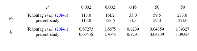
 Rec
 λi
 χ=104
 I∗
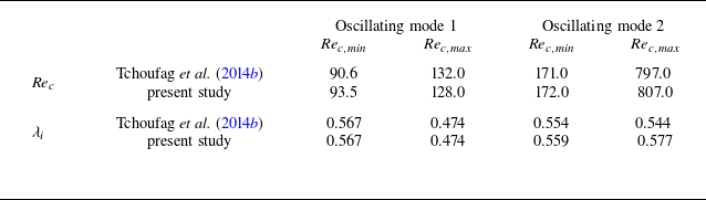
 Rec,min
 Rec,max
 λi
 χ=2.5

 (χ,I∗,Re)=(3,0.56,298)
 (a)
 (b)

 (Re,ρ∗)=(100,2.546)
 ρ∗
 (a)
 (b)
 U∗
 (c)
 St=λid/(2πU∞)
 U∗

 χ=1.9
 (a)
 λr
 Re
 S
 (b)

 (a)
 ΘLB=0∘
 ΘTB=8∘
 (χ,S,Sr)=(1.6,3,0.1)
 (b)

 (Re,S)
 χ=1.9
 (a)

 χ
 χLB=1.9
 (a)
 (χLB,χTB)=(1.9,1.7)
 (b)
 (χLB,χTB)=(1.9,1.8)
 χ
 χLB=χTB=1.7
 1.8
 1.9
 χ
 (1.9,1.7)
 (1.9,1.8)

 (a)
 χ=1.6
 (b)
 (Re,S)
 a1/a2≃0.94
 (a)


