INTRODUCTION
Modern varieties of wheat grown in temperate regions require the application of nitrogen (N) fertilizer to realize their yield potential. The fertilizer can increase both yields and profitability for farmers. However, it not only increases agricultural yields but can also damage the environment, both globally and locally (Sutton et al. Reference Sutton, Howard, Erisman, Billen, Bleeker, Grennfelt, Van Grinsven and Grizzetti2011). Excess N can be transformed to nitrous oxide and emitted into the atmosphere, and leaching of nitrate can cause eutrophication in lakes and rivers. Nitrogen fertilizer is estimated to be responsible for c. 0·70 of the emissions of greenhouse gas from wheat production (Berry et al. Reference Berry, Kindred, Olesen, Jorgensen and Paveley2010). Hence, both farmers and governments have an interest in ensuring that fertilizer N is applied to maximum efficiency. There are guidelines and decision-support systems to help farmers decide how much fertilizer to apply, but these are disappointingly ineffective (Sylvester-Bradley et al. Reference Sylvester-Bradley, Kindred, Blake, Dyer and Sinclair2008; Kindred et al. Reference Kindred, Knight, Berry, Sylvester-Bradley, Hatley, Morris, Hoad and White2012).
For many years, the rates of fertilizer were determined for individual fields, but modern technology and machines enable farmers to vary their applications of fertilizer at as fine a resolution as 10m×10m. Agronomists have therefore sought to estimate the N requirement at the same spatial resolution (Heege et al. Reference Heege, Reusch and Thiessen2008).
Since the 1970s, the optimum applications of fertilizer N for individual experiments have been determined empirically from data on the response of the yield to a range of rates of fertilizer N (including zero). This has been achieved by the fitting of response curves to yield data as functions of applied N, and then interpolation of the point at which the profit to the farmer is maximized (Boyd et al. Reference Boyd, Yuen and Needham1976). This point is the optimum N requirement (N opt). The point depends on two factors external to each crop experiment, namely the choice of the fitted curve and the relative price of grain to fertilizer N (the break-even ratio: BER). The BER describes the weight of grain required to pay for a given weight of fertilizer N, and is typically around 5 : 1, but it has varied between 2 : 1 and 9 : 1 in recent decades (Sylvester-Bradley & Kindred Reference Sylvester-Bradley and Kindred2009). The economic optimum is the point on the response curve at which the slope equals the BER; i.e. the point at which increasing the fertilizer N applied by 1 unit would not increase grain yields sufficiently to pay for the cost of that fertilizer.
National recommendations for N fertilizer are based on the accumulated evidence of numerous experiments on N response (Defra 2010). Implicit in these recommendations are three underlying principles, as follows.
-
1 Crop N demand (CND). The crop demands N from the soil so that it can create enough photosynthetic material (i.e. leaves and stem) to maximize its production of dry matter (Grindlay Reference Grindlay1997; Lemaire et al. Reference Lemaire, Van Oosterom, Sheehy, Jeuffroy, Massignam and Rossato2007). It also demands N to satisfy protein deposition in the grain (Pask et al. Reference Pask, Sylvester-Bradley, Jamieson and Foulkes2012). In wheat crops yielding >9 t/ha with grain protein of 110 g/kg dry matter, the demand for N for grain protein tends to exceed that for photosynthesis.
-
2 Soil N supply (SNS). Nitrogen derived from the soil comes from the residues of previous crops and the mineralization of organic matter (plus that from atmospheric deposition). It tends to be the most variable component of the N requirement (Kindred et al. Reference Kindred, Knight, Berry, Sylvester-Bradley, Hatley, Morris, Hoad and White2012), and its prediction is the focus of most recommendation systems.
-
3 Fertilizer N recovery (FNR). The difference between the CND and the SNS is the N that needs to be supplied in the fertilizer for the crop to fulfil its potential. Fertilizer N is usually recovered with much less than 100% efficiency. The efficiency, expressed as a percentage, is known as the FNR and is on average c. 60% (Bloom et al. Reference Bloom, Sylvester-Bradley, Vaidyanathan, Murray, Jenkinson and Smith1988). Thus, the fertilizer N needed to fulfil the crop's demand (the fertilizer N requirement, F) is given by
(1) $$F = \displaystyle{{{\rm CND} - {\rm SNS}} \over {{\rm FNR}}}$$

The crop's demand for N and the SNS can be quantified from the crop measurements. The N taken up by the crop (crop N uptake) increases almost linearly with the rate of N applied to a maximum, which represents the crop N demand (CND) (Bloom et al. Reference Bloom, Sylvester-Bradley, Vaidyanathan, Murray, Jenkinson and Smith1988; Sylvester-Bradley & Kindred Reference Sylvester-Bradley and Kindred2009). Adding more fertilizer N past this point will not result in an increase in the amount of N taken up by the crop. The N taken up by this fertilized crop can be used to estimate the CND. The N taken up by an unfertilized crop, termed ‘the harvested SNS’, can be used as an estimate of the SNS.
Fertilizer N recovery (FNR), which is the proportion of the added fertilizer taken up by the crop, is the most problematic of the components to calculate. Without adding 15N-labelled fertilizer, one cannot distinguish N in the crop derived from the fertilizer from that from the soil. Even with the use of labelled fertilizer the interchangeability of soil N and fertilizer N makes interpretation difficult. Fertilizer recovery for a given rate of applied N is therefore normally given as the apparent fertilizer recovery (AFR); it is calculated from the N taken up by the crop with N applied minus crop N uptake with nil-N (harvested SNS) divided by the rate of applied N (Bloom et al. Reference Bloom, Sylvester-Bradley, Vaidyanathan, Murray, Jenkinson and Smith1988).
The AFR evidently depends on the estimates of the SNS, and it is implicitly assumed that the recovery of soil N remains constant as fertilizer N is applied. There is also the difficulty that the fertilizer recovery depends on the quantity of N applied. It is generally found that the response of the crop to initial additions of N is linear and then declines until it is zero once the crop's demand for N has been satisfied (beyond this point there is no increase in the N uptake no matter how much N is applied).
One can estimate CND, SNS and AFR by fitting a model to the data on the N uptake from the experiments on N response. The model most commonly used is a split-line model, with the slope of the second line constrained to zero, (Kindred et al. Reference Kindred, Knight, Berry, Sylvester-Bradley, Hatley, Morris, Hoad and White2012; Sylvester-Bradley et al. Reference Sylvester-Bradley and Withers2013):
 $$\eqalign{z& = \alpha + \beta N,\quad {\rm when}\,\alpha + \beta N \lt \gamma \cr z& = \gamma, \quad {\rm otherwise}} $$
where z is the crop N uptake and N is the fertilizer N applied. The parameters α, β and γ represent the SNS, the AFR and the CND, respectively.
Kindred et al. (Reference Kindred, Knight, Berry, Sylvester-Bradley, Hatley, Morris, Hoad and White2012) explored the components of the N requirement at a national scale using data from the earlier experiments on N responses. The current study, however, is concerned with the variation in N requirement and its underlying components within fields; the local response to N therefore had to be quantified. In other studies, the investigators have taken a similar approach (Lark & Wheeler Reference Lark and Wheeler2003; Pringle et al. Reference Pringle, Mcbratney and Cook2004; Bishop & Lark Reference Bishop and Lark2006). The approach offers the opportunity to understand the variation in N requirement and its causes, without the normal confounding differences in management, weather, variety, previous crop history, etc.
‘Checkerboard’ experiments (described below) enabled the spatial variation in N requirements to be examined. The variation in the SNS, the CND and the AFR were examined along with their relationships with one another and their relationship to the optimum fertilizer application (N opt) at the three sites in two seasons. Thus, several hypotheses relating to fertilizer recommendations could be explored, as follows.
-
1. If a crop has a large demand for N then
-
(a) either it warrants a larger application of fertilizer N, or
-
(b) the CND is positively related to fertilizer recovery or the SNS, thereby tempering the extra requirement for N.
-
-
2. As the SNS increases so
-
(a) the optimum N requirement diminishes in direct proportion modified by the recovery of fertilizer N, or
-
(b) the recovery of the SNS reduces (Knight et al. Reference Knight, Macdonald, Glendining, Whitmore, Dailey, Goulding, Sinclair and Rees2008) and so tempers the effect of the differences in the SNS on N requirements.
-
-
3. The protein content of the grain remains fairly constant when optimum N is applied. This means that the measurements of protein can indicate successful fertilizer management (Sylvester-Bradley & Clarke Reference Sylvester-Bradley and Clarke2009).
MATERIALS AND METHODS
The experimental designs
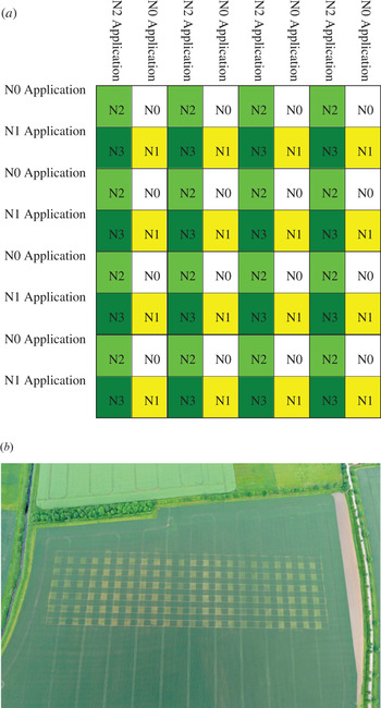
The experiments were laid out on three commercial fields in England (the design is shown in Fig. 1). Two of the fields were on Hall Farm at Flawborough, Nottinghamshire (52°58′N, 0°50′W) and are referred to here as F1 and F2. The third was on Signet Hill Farm at Burford, Oxfordshire (51°48′N, 1°40′W) and is referred to as B1. In each experiment, winter wheat was grown with cultivars Alchemy (on F1), Duxford (on F2) and Solstice (on B1). The HGCA Recommended List (HGCA 2013) shows the varieties to have similar yield potential (98, 100 and 96% of a control, respectively). Alchemy and Duxford are feed varieties, whereas Solstice is a milling variety with a larger protein content (111, 108 and 118 g/kg dry matter, respectively), which would be expected to need as much as 20 kg/ha more fertilizer N (Sylvester-Bradley Reference Sylvester-Bradley2009).
(a) The design of the chequerboard experiment in field F1 at Flawborough. The plots were fertilized with either 0, 120, 240 or 360 kg N/ha; (b) An aerial photograph of Flawborough field F1 during the chequerboard experiment (Colour version available online).

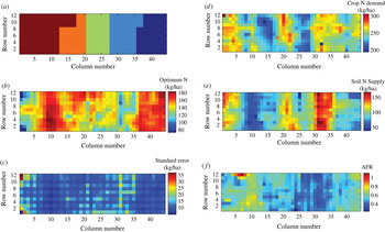
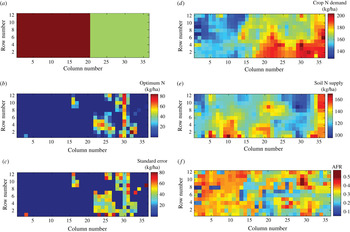
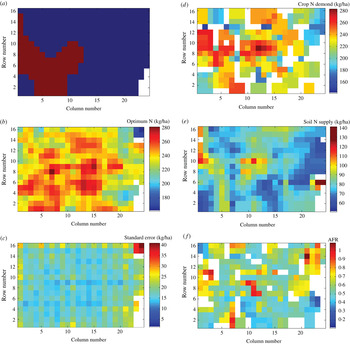
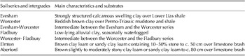
The soil at Flawborough is dominantly clay loam. In field F1 it is of the Evesham, Worcester and Fladbury series (Table 1). In Field F2, adjacent to field F1, the soil is also clay of the Worcester and Fladbury series. The soil in Field B1 is typical of large areas on the Jurassic limestones, known locally as ‘Cotswold brash’. Most is fairly thin brown calcareous clay loam containing numerous limestone fragments (Elmton series, Table 1). The experiment lies across the head of a dry valley in which the soil is considerably deeper (Aberford series, Table 1). The soil series across each experiment are shown in Figs 2(a) (F1), 3(a) (F2) and 4(a) (B1).
Field 1. (a) The soil series, from left to right, Fladbury, Worcester–Fladbury, Worcester, Worcester–Evesham and Evesham; (b) the optimum N; (c) the s.e. of the optimum N; (d) estimates of the CND; (e) estimates of the SNS; and (f) model based estimates of the AFR (Colour version available online).

Field F2. (a) The soil series, from left to right, Fladbury, Worcester; (b) the optimum N; (c) the s.e. of the optimum N; (d) the estimates of the CND; (e) the estimates of the SNS; and (f) model based estimates of the AFR (Colour version available online).

Field B1. (a) The soil series are Elmton and Aberford (Y-shaped valley); (b) the optimum N; (c) the s.e. of the optimum N; (d) the estimates of the CND; (e) the estimates of the SNS; and (f) the model based estimates of the AFR (Colour version available online).

Soil types at Flawborough and Burford and their characteristics

See Ragg et al. (Reference Ragg, Beard, George, Heaven, Hollis, Jones, Palmer, Reeve, Robson and Whitfield1984) and Jarvis et al. (Reference Jarvis, Allen, Fordham, Hazelden, Moffat and Sturdy1984) for more details.
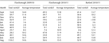
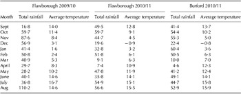
Table 2 summarizes the weather at Flawborough and Burford during the seasons when the experiments were performed.
Average temperatures (°C) and total rainfall (mm) at Flawborough during seasons 2009/10 and 2010/11 and at Burford during season 2010/11
The basic design of the experiments was that of a checkerboard (Pringle et al. Reference Pringle, Mcbratney and Cook2004) of contiguous square plots, c. 10 m on each side. The plots were grouped into sets of four, and in each set, four levels of N, one of which was nil, were applied in a fixed pattern (Fig. 1(a)). The actual amounts applied varied according to the judged requirement of the crop after the mineral N in the soil had been measured in the spring. Soil samples on which to determine mineral N were taken from at least 15 positions in each experiment. Sample points were chosen to cover the expected variation in the field. Average soil mineral N results were 36 kg/ha at F1 (range 24–56 kg/ha, s.d. 8·3 kg/ha), 108 kg/ha at F2 (range 63–157 kg/ha, s.d. 30 kg/ha) and 63 kg/ha at B1 (range 34–104 kg/ha, s.d. 18·9 kg/ha). Therefore, on fields F1 and B1, the plots were fertilized with either 0, 120, 240 or 360 kg N/ha and on field F2, where the optimum was expected to be less, the plots were fertilized with either 0, 100, 200 or 300 kg N/ha. In each experiment, fertilizer was applied as Chafer Nuram 37 liquid (urea and ammonium nitrate) with a conventional farm sprayer. At each site, the total amount of fertilizer was applied in two equal portions, one in March and one in April. On each application date, the sprayer crossed the field twice, with the second set of passes perpendicular to the first. On the first pass, half the boom applied no N (N0) and the other half applied N at rate 1 (N1). On the second perpendicular pass, again half the boom applied no N and the other half applied N at rate 2 (N2). This resulted in four rates of N: rates 0 (N0+N0), 1 (N1+N0), 2 (N0+N2) and 3 (N1+N2).
The experiment on field F1 was done in the 2010/11 season and was imposed on the field in a rectangular strip of 12×44=528 plots, each 10m×10m (Fig. 1(b)). The other two experiments were done in season 2011/12 with an experimental protocol and design similar to that used in field F1. In field F2, the experimental plots were in a rectangular strip of 12×36=432 plots, each 9m×9m. To capture the full variation in field B1, a rectangular strip of 16×22 plots, 11m×11m was imposed on the field with an additional two strips of 13 and 11 plots down one side (Fig. 4(a)), giving a total of 376 plots.
In all the three experiments, the wheat was harvested with a Sampo Rosenlew SR2025 plot combine harvester and grain yield was measured. To eliminate any effect of harvesting direction being confounded with treatment, two cuts were taken in opposite directions and the yields were averaged. The moisture content of each sample of grain was measured with a Dickey–John moisture meter, and the measured yields were corrected to 850 g/kg dry matter. Protein (as g/kg dry matter) was measured on one sample of grain from each plot with a FOSS Infratec NIR analyser. Before harvest, grab samples of c. 100 shoots were taken from each plot. The shoots were counted, and the ears were separated from the straw, dried and weighed. The ears were then threshed, and grain was weighed. From these measurements, the harvest index for each plot was estimated by division of the grain dry matter per shoot by the total dry matter per shoot, and the proportion of N in the straw was determined by the Dumas method. With these measurements together with the combine grain yield and the grain protein, the N taken up in the grain was estimated by multiplying the grain yield by the proportion of protein in the grain and dividing by 5·7, which is the conversion factor in wheat for converting grain N (g/kg) to grain protein content (g/kg).
The N harvest index was estimated by division of the grain N per shoot by the total N per shoot. Finally, total N uptake was estimated by division of the N in the grain by the N harvest index.
Calculating the optimum nitrogen requirement
Response models were fitted to the local yield measurements from within windows of size 3×3 plots. These were used to estimate the optimum N (N opt ) for each plot. It was assumed that the fitted response model represents the behaviour of the central plot, i.e. a response for a given plot was based on the measurement from the plot itself and the measurements from the neighbouring plots. The fitted responses for the plots that lay at the edge of the experiment were necessarily based on fewer measurements. The exponential equation was chosen as the model:
 $$y_p = a_p + b_p R_p^N, \quad {\rm for}\;p = 1,2, \ldots, n$$
Here, y p is yield (t/ha), N is applied N (kg/ha), n is the number of plots and a p , bp and R p are the parameters fitted to the data assigned to plot p. This model is used widely, but sometimes it is generalized by addition of an extra term c p N, where c p is another parameter. This generalization allows for loss of yield at larger rates of N, which sometimes occurs because of lodging, increased susceptibility to disease, greater respiration or less efficient photosynthesis. To avoid overfitting and because the yield at the largest rate of fertilizer (360 or 300 kg/ha) was never much less than the yield at the 240 or 200 kg/ha rate, the simpler model was chosen.
In addition, because the model was fitted to few data, the parameter R p was kept constant for any one field (denoted R). Fixing this parameter is a common practice in the analysis of the experiments on the response of crops to N in Britain (Lark & Wheeler Reference Lark and Wheeler2003) and has little effect on the goodness of fit. The yield response model was fitted with the GenStat directive fitnonlinear (Payne et al. Reference Payne, Harding, Murray, Soutar, Baird, Glaser, Welham, Gilmour, Thompson and Webster2011), and this gave estimates for the parameters a p , bp and R for p=1, 2,…,n with associated s.e.
Given a yield response function and the prices for N fertilizer and wheat grain, the optimum rate of N fertilizer can be calculated as:
 $$N_{{\rm opt}} = \ln (R)\ln \left\{ {\displaystyle{{{\rm BER} \times \ln (R)} \over {1000\,b_p}}} \right\},\quad {\rm for}\;p = 1,2, \ldots, n$$
A BER of 7 : 1 based on a wheat price of £150 per t and a price for N fertilizer of £1·05 per kg were used, and the GenStat directive rfunction was used to estimate the N optimum for each plot and the associated s.e.
Identifying the components of the requirement for fertilizer nitrogen
To estimate the three components of the fertilizer-N requirement, F in Eqn (1), the local response in N taken up by the crop to the application of N fertilizer first had to be estimated. A split line model was fitted, given in Eqn (5) below, to measurements of N taken up in the crop from within the local windows of size 3×3 plots, and it was assumed that the fitted response model represents the behaviour of the central plot:
 $$\eqalign{z_p & = \alpha _p + \beta _p N,\;{\rm when}\,\alpha _p + \beta _p N \lt \gamma _p \cr z_p &= \gamma _p \,{\rm otherwise};\;{\rm for}\,\,p = 1,2, \ldots, n} $$
Here, z p is the crop N uptake on plot p, N is applied N (kg/ha), n is the number of plots, and α p , βp and γ p are the parameters, fitted to the data assigned to plot p. Each of the parameters represents a component of the fertilizer N requirement of the crop: α p is the SNS on plot p, β p is the AFR on plot p, and γ p is the CND on that plot.
The relationship between the components of the fertilizer nitrogen requirement and optimum nitrogen
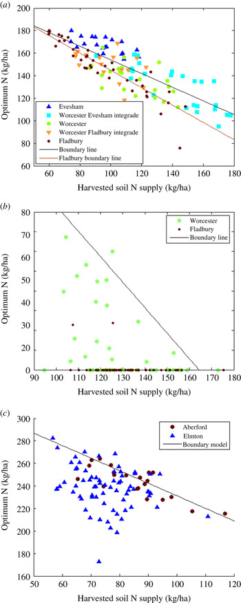
Each of the components of fertilizer N requirement was treated as an explanatory variable for the observed response in optimum N. Where there appeared to be a relationship between optimum N and the components of the fertilizer N requirement and the explanatory variable boundary-line models were fitted. The boundary-line model, first proposed by Webb (Reference Webb1972), describes sets of data in which one variable (the explanatory variable) appears to limit the response of the other (the response variable). The concept is that there is some upper limit (or boundary) to the value of the response variable at any given value of the independent variable so that values larger than the boundary are impossible (apart from error). Data points lying below the boundary are limited by other factors.
In the current context, optimum N is the response variable, and one of the components of the N requirement (e.g. CND) is the explanatory variable. The boundary line describes the relationship between the two. Scatter below the boundary line results from factors other than the explanatory variable having a substantial limiting influence on optimum N. If no other variable substantially limits the response variable, however, then the boundary line will go through the middle of the scatter more akin to a regression model.
The method of Milne et al. (Reference Milne, Ferguson and Lark2006) was used to fit the boundary-line models which effectively describe censored bivariate probability distributions. The censor in the distribution is the boundary line, and a parameter of variation quantifies the error around the boundary line. The censored bivariate distribution is fitted to the data by maximum likelihood. Akaike's information criterion (AIC) (Akaike Reference Akaike, Petrov and Csáki1973) was used to assess whether the boundary line model represented the relationship better than a bivariate normal model. The AIC allows the comparison of models based on a compromise between parsimony and goodness of fit (which usually improves with increasing numbers of parameters). The AIC for any given set of data can be represented by
 $${\rm AIC} = -2 \ln M + {\rm 2}Q $$
where M is the maximum likelihood value and Q is the number of parameters in the model. When comparing two or more models with the same number of parameters one will favour the one with the largest likelihood; that model will also have the smallest AIC. If the models have different number of parameters then the one with the smallest AIC is the most appropriate, regardless of the size of M. Milne et al. (Reference Milne, Ferguson and Lark2006) expanded on this in the context of boundary-line fitting. In the instances where the boundary-line model was not the best, linear regression models were fitted to the data and soil type was treated as a factor to see if there was any evidence that the relationship changes with differences in the soil type.
Crop N demand
A positive response was expected between the demand for N by the crop and the optimum application of N, because where the demand is smaller the optimum for applied N will also be smaller. To investigate the relationship between the CND and the optimum N, the optimum N was plotted against the crop N uptake obtained at the maximum fertilizer rate (i.e. 360 kg N/ha for field F1, 300 kg N/ha for field F2 and 360 kg N/ha for field B1). These rates of fertilizer N span the maximum value attainable by the crop.
Soil N supply
A negative relationship between the N supply from the soil and the optimum N was expected. To confirm, optimum N was plotted against the harvested SNS.
Fertilizer N recovery
Fertilizer N recovery was expected to be negatively related to optimum N, because optimum N should decrease with the increasing efficiency of the use of the fertilizer. No direct measurements that related to FNR were available, and hence instead, the model in Eqn (5) was fitted to provide an estimate of AFR, the apparent fertilizer recovery.
RESULTS
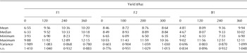
All the three sites showed large variation in grain yield (Table 3), with yields at one N level varying by >4·5 t/ha at each site. At sites F1 and B1 the unfertilized yields varied even more. The application of the N fertilizer increased the average yield by 3·8 t/ha at F1 and by more than 5 t/ha at B1, but at site F2 fertilizer increased the average yield by only 0·3 t/ha.
Summary statistics of the yield data at four rates of fertilizer N (kg/ha) in fields F1, F2 and B1

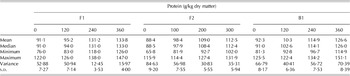
Grain protein content at one N level varied by c. 2% at site F1 and by >3% (on a dry-matter basis) at sites F2 and B1 (Table 4). The application of the N fertilizer increased the average grain protein content at each site, by >4% at site F1, 2·4% at site F2 and 3·4% at site B1. Notably, despite the small response of yield to the applied N in field F2, the increase in the grain protein in response to the applied N was similar to those in the other two fields.
Summary statistics of the grain protein data at four rates for fertilizer N (kg/ha) in fields F1, F2 and B1

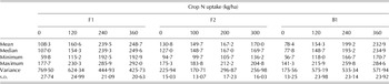
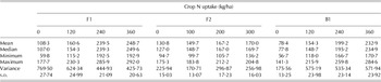
Table 5 summarizes the crop's uptake of N for each of the treatments in each of the fields. The average amount of N in the harvested crop on the unfertilized plots at site F2 was larger than the averages at the other two sites. The response to the applied N was small at site F2, however, and the average at the maximum rate (170 kg/ha) was much smaller than the average at sites F1 and B1 (248 and 233 kg/ha respectively).
Summary statistics of the crop N uptake at four rates for fertilizer N (kg/ha) in fields F1, F2 and B1
Estimating optimum nitrogen
The fitted N optima for the sites are shown in Figs 2(b) (F1), 3(b) (F2) and 4(b) (B1), and the associated s.e. are shown in Figs 2(c) (F1), 3(c) (F2) and 4(c) (B1). s.e. can be used to indicate the relative uncertainties of the parameter estimates. Here, however, the calculated s.e. will be somewhat biased because the surveys were systematic rather than probabilistic. Where the s.e. are large, however, there is strong evidence that the parameter estimates are uncertain. Table 6 summarizes the estimates of optimum N. One of the plots in F1 (row 1, column 1) and three of the plots in B1 (row 14, columns 23 and 24, and row 6, column 23) were over-fertilized, hence, a reliable value for the optimum could not be estimated for them. Nor could an N response curve be fitted for the large areas of site F2, and hence again an optimum could not be determined. Therefore, the R parameter was fixed at 0·995. This value is commonly used in modelling the responses of wheat to N in Britain (Sylvester-Bradley et al. Reference Sylvester-Bradley, Kindred, Wynn, Thorman and Smith2012) and is similar to that found in the other two trials of the current study.
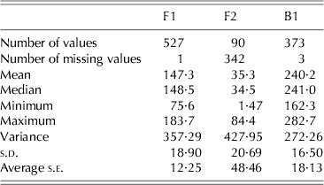
Summary statistics of the estimated optimum N (in kg/ha) for fields F1, F2 and B1

Plots where the optimum N was zero or where overfertilization meant that the optima could not be reliably calculated have been excluded.
The range in optimum N obtained from the fitting was substantial at all the sites (Table 6), but it was largest at sites F1 and B1 where it exceeded 100 kg/ha. At site F2, where the soil contained more mineral N, the s.e. for the optimum N were large and the estimates of the N optima were very uncertain there.
There was an apparent relationship between the soil series and the N optima at sites F1 and F2. At site F1, the optima on the Evesham series were larger than those of the neighbouring Worcester-Evesham intergrade, as is evident on the right-hand sides of Figs 2(a) and (b). At site F2, the optima that were > zero tended to be on the Worcester series (Fig. 5(b)). There was no evident relation between the optimum N and the soil series at site B1.
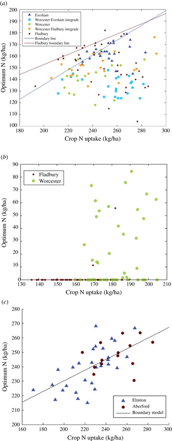
The optimum N plotted against the crop N uptake with (a) 360 kg N/ha in field F1, (b) 300 kg N/ha in field F2, and (c) 360 kg N/ha in field B1, with the fitted models. The model parameters are reported in Table 7 (Colour version available online).

The components of the fertilizer nitrogen requirement
Field F1
Figure 2 shows the estimates of the CND (d), the SNS (e), and the AFR (f) derived by fitting Eqn (5) to the data. The spatial variation in the CND and the SNS are broadly similar. Where the demand is large the supply tends to be large also, and vice versa. The map of the AFR shows that generally the greatest values occur on the Fladbury and the Evesham soils. Of the three components, the map of the SNS most closely resembles the map of the optimum N, suggesting that the SNS influences the optimum N the most.
Field F2
Similarly, Fig. 3 shows the estimates of the CND (d), the SNS (e) and the AFR (f) derived by fitting Eqn (5) to the data from field F2. Figure 3(d) shows that the largest demand for N was on the Worcester soil, which was where the positive values of the optimum N were concentrated. Across the Worcester soil there was some similarity between the map of N supply and the map of the optimum N across this soil. The spatial variations in the CND and the AFR are broadly similar. Where the CND was large the AFR tends to be small, and vice versa.
Field B1
Figure 4 shows the estimates of the CND (d), the SNS (e) and the AFR (f) derived by the fitting of Eqn (5) to the data of field B1. Financial constraints meant that only 227 of the 376 grab samples could be analysed for N content and harvest index; and hence the model could not be fitted nor the components for N requirement be estimated for all the plots. In the figures, the plots for which no estimates were available are left white. The CND was largest on the Aberford soil. Not surprisingly, the larger values for the N supply were mainly in the dry valley where the soil is deepest. Visually, there was little coherent spatial pattern in the estimates for the AFR (Fig. 4(f)); the neighbouring plots tended to have similar values whereas the ones further away differed more.
The relationship between crop nitrogen demand and optimum N
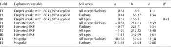
Crop N demand was estimated from crop N uptake as described above. Figure 5 shows the optimum N plotted against the crop N uptake with (a) 360 kg N/ha in field F1, (b) 300 kg N/ha in field F2, and (c) 360 kg N/ha in field B1. Evidently, the data displayed in Fig. 5(a) conforms to a boundary-line model, and this was supported by the AIC. Two boundary-line models were considered. The first describes all the data, and the second has a separate model for the Fladbury series (which appears to have a boundary higher in the scatter than the rest of the data). The AIC indicates that a separate boundary line suits the Fladbury data better. The modelled boundary lines are shown in the figure, and the parameters are listed in Table 7. Figure 5(a) shows most of the scatter to lie below the fitted boundary lines and that on most of the plots the optima were limited by factors other than the demand for N by the crop.
Parameters for the predictors of the optimum N, obtained from the boundary-line analysis or by simple linear regression
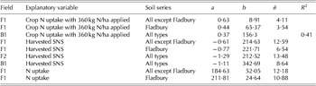
The error associated with the boundary line (σ) and the R 2 values for the regression lines are also reported.
The data in Fig. 5(b) show little relationship between the variables, and hence a model was not fitted. It is clear, however, that the optimum N was rarely larger than zero on the Fladbury soil.
There is an apparent boundary in the data plotted in Fig. 5(c). According to the AIC, however, a bivariate normal model described the data better than a boundary-line model. An accumulated analysis of variance showed that separate models should not be fitted for each soil type. The fitted model is plotted in Fig. 5(c), and Table 7 reports the parameter values, together with R 2.
The relationship between the soil nitrogen supply and the optimum nitrogen
Soil N supply was estimated from the crop N uptake as described above. Figure 6 shows the optimum N (in kg/ha) plotted against the crop N uptake where no fertilizer N was applied (harvested SNS) for (a) field F1, (b) field F2 and (c) field B1. The fitted models are also shown, and their parameters are reported in Tables 7. In each case, the AIC supported a boundary-line model over a bivariate normal model. For field F1 (Fig. 6(a)), the AIC suggested a separate boundary-line model for the data from the Fladbury soil. Most of the scatter lies around the fitted boundary lines, showing that factors other than SNS have little effect on optimum N. The boundary-line analysis of the data from site F2 supported the observation that on the Worcester soil the supply of N from the soil (SNS) was important in determining the N optima. For field B1, the measurements made on the Aberford soil tend to cluster around the boundary, suggesting that on this soil, factors other than SNS did not substantially limit optimum N.
The optimum N (in kg N/ha) plotted against the harvested SNS (in kg N/ha) for fields (a) F1, (b) F2 and (c) B1, with the fitted models. The model parameters are reported in Table 7 (Colour version available online).

The relationship between the apparent fertilizer recovery and the optimum nitrogen
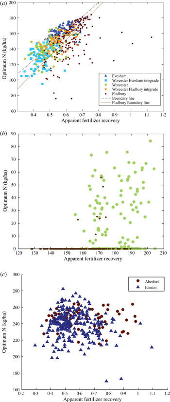
The model in Eqn (5) was fitted to the data to provide the estimates of the AFR. Figure 7 shows the optimum N plotted against the estimated AFR for each field. There were no direct measurements of the AFR, only model estimates, and hence one must be cautious when interpreting the results. According to the AICs the data in Fig. 7(a) conformed to a boundary-line model with a separate boundary line to describe the data from the Fladbury soil. The boundary lines are shown on the figure, and the parameters are given in Table 7. The relationship between the AFR and the optimum N was expected to be negative, but here it was positive. This could be an artefact of the model fitting or a result of an interaction between the SNS and the AFR.
The optimum N (kg N/ha) plotted against the estimated AFR for field (a) F1 with the fitted model, (b) F2 and (c) B1. The model parameters are reported in Table 7 (Colour version available online).

There was no evident relationship between the optimum N and the AFR at site F2 or site B1, Figs 7(b) and (c).
DISCUSSION
At all the three sites, the optimum fertilizer dressings varied substantially across the fields (typically by c. 100 kg N/ha). Lark & Wheeler (Reference Lark and Wheeler2003) found a similar result for a field in southern England. At site F2, the poor response in yield to applied fertilizer resulted in large s.e. which means that the estimates of the N optima are only rough, but one can be sure that the N requirements there are small (<100 kg N/ha). Experiments showing little or no yield response to fertilizer N are fairly common in the UK. For example, Sylvester-Bradley et al. (Reference Sylvester-Bradley, Kindred, Blake, Dyer and Sinclair2008) found that winter wheat did not respond to added N in six out of the 30 experiments; they were usually able to attribute this lack of response to a large supply of N from the soil. A similar explanation can account for the current observations at site F2, where there was a large amount of mineral N in the soil (60–140 kg/ha).
The response to fertilizer N, however, can depend on the weather, and the poor response at Flawborough in 2011 was probably caused by drought. There was little rain there during March, April and May compared with the long-term average of 160·5 mm. This lack of rain severely limited the uptake of fertilizer N and limited crop growth and tillering. The warm, dry conditions increased the likelihood of loss of fertilizer N through volatilization of ammonia. The drought is likely to have killed much of the soil's micro-flora, and rapid mineralization of N caused by rewetting in late May and June was too late to increase yields substantially; there were too few shoots and leaves to intercept light and photosynthesize. Nitrogen was taken up, however, and this increased protein in the grain.
The variation in the N optima at site F1 is spatially coherent and visually matches the trends in variation of the SNS, the CND, the AFR and the underlying soil series. The variation in the optimum N was predominantly due to the variation in the SNS.
Clearly, there are interactions between the three components at site F1 and the importance of the CND and the AFR in determining the requirement for N should be recognized. If a crop's demands for N and the AFR were constant across the field then a difference in N supply of 100 kg/ha from the soil would result in a difference in the requirement from the fertilizer of 100/AFR kg per ha. For example, an AFR of 0·6 would be equivalent to 167 kg/ha, and here there is a difference of only c. 100 kg/ha. Surprisingly, the areas with the largest supply of N in the soil were where the crop's demand was largest. It seems that the other attributes of the soil (more water, more of the other plant nutrients and better aeration) have helped to make more N available to the crops and hence boost yields and demand for N.
Measurements of soil mineral N made in the spring showed little variation (30–60 kg/ha) with no strong spatial coherence. It was surprising, therefore, to see the large variation in the harvested SNS. The cause for such large spatial differences in the SNS is unknown; there are no clear differences in soil organic matter or soil total N to indicate differences in mineralization, yet in certain areas of the field, the crop accessed much more N from the soil. The parts of the field where the SNS was largest were where in past years the yield was also the largest (Milne et al. Reference Milne, Webster, Ginsberg and Kindred2012). The greater crop growth in these areas could have left more organic matter to accumulate in the soil and to mineralize and release N. It is hard to believe that such a process would supply much N from the soil, and so perhaps the large harvested SNS is manifest only because fertilizer was withheld. Nevertheless, it is a matter that merits further investigation.
At site F2, the N optima that were larger than zero were mostly on the plots of the Worcester soil that supplied little N. Across the Worcester series, the variation in N optima visually matched trends in variation seen in the SNS. The boundary-line analysis confirmed that the shortage of N there increased the N optima.
Site B1 has a Y-shaped valley where the soil is much deeper than elsewhere in the field (>90 cm compared with 30–40 cm elsewhere). The soil is of the Aberford series and yields more than the thinner soil elsewhere. The pattern of the N optima for the site is spatially coherent, but cannot be matched to the patterns of the SNS, the CND, the AFR or the soil series. The boundary-line analyses help elucidate the factors controlling the optimum N somewhat. In particular, the relation between the CND and the optimum N, and the relation between the SNS and the optimum N are clearer. The points below the boundary line are of the sites where the other factors are limiting the optimum N. The sites on the Aberford soil lie close to the boundary, suggesting that there the SNS largely determined the optimum N. Elsewhere, the CND seemed equally important. There was little evidence that fertilizer recovery played a major role in the differences in N requirement, yet the variation in the AFR was very large (0·3 to >1).
The three questions for which the experiments were designed are discussed below.
1. To what extent should the demand for N by the crop determine fertilizer recommendations?
The results show that the greater is the demand for N by the crop, the more fertilizer N should be applied. However, the effect is tempered by the interaction of the crop's demand for N with the N supplied by the soil and the fertilizer recovery. The relative importance of these factors varies from site to site and within sites, generally as a function of soil type. Knowing only one component is not enough; all the components must be considered together to predict N fertilizer requirement with reasonable precision. Interactions between the components can vary from place to place. No evidence was found that the CND was positively related to fertilizer recovery. A new finding was the association between the crop's demand for N and the ability of the soil to supply it. This association should therefore be taken into account in the calculation of spatially variable requirements for N.
2. How important is the soil's ability to supply nitrogen?
The most important component determining fertilizer requirement was found to be the SNS at all the three sites. There was also evidence that the SNS was inversely related to fertilizer recovery.
Unfortunately, current methods for predicting SNS are unsatisfactory (Kindred et al. Reference Kindred, Knight, Berry, Sylvester-Bradley, Hatley, Morris, Hoad and White2012). ‘Field assessment’ (based on soil type and previous crop) is quick, cheap and correct on average, but it explains only about a third of the field-to-field variation, and it can rarely be used to predict variation within fields. Tests for mineral N in the soil are more precise and precision and accuracy might be improved with the assessments of mineralization; but it still does not predict more than half of the field-to-field variation and it is too costly to use repeatedly within fields (Marchant et al. Reference Marchant, Dailey and Lark2012). New ways for assessing the SNS must therefore be sought by, for example canopy sensing, either via satellite, from the air or from sensors mounted on tractors. Such systems are already used by precision farmers, but not currently to estimate N supply directly. Sylvester-Bradley et al. (Reference Sylvester-Bradley, Wiltshire, Kindred, Hatley and Clarke2009) showed that one can quantify the SNS with reflectance measures by comparing NDVI of a given crop with that expected from a crop of the same age (in thermal time) that is unlimited for N. This approach needs much development and validation, but it does offer a chance of obtaining independent estimates of the SNS that are spatially variable.
3. How variable is the grain protein when the optimum N is applied?
The grain protein achieved when the crop is fertilized for a financially optimum yield is reported to be consistently around 110 g/kg for the feed varieties (Sylvester-Bradley & Clarke Reference Sylvester-Bradley and Clarke2009). The results for fields F1 and B1 are in accord with this. Across most of field F2 the optimum N was zero; where it was not so, the average for the optimum was 35·3 kg N/ha (see Table 6). At these fertilizer rates the average grain protein was closer to 90 g/kg.
CONCLUSION
The experiments described above and those of the other investigators (e.g. Lark & Wheeler Reference Lark and Wheeler2003) show that there is substantial variation in the requirements for fertilizer N within fields and that these can be understood in terms of differences in the crops’ demands for N (CND) and the supply of N from the soil (SNS). The positive relationship that was observed in the current work between the crop's demand for N and the N supplied by the SNS within the field is an important new consideration for farmers wishing to economize by varying the amount of fertilizer N they apply. The large variation in fertilizer recovery and absence of any plausible relationship with the N optima requires further examination. It needs to be understood so that farmers can improve fertilizer recovery and the use of fertilizer to obtain larger yields without greater inputs (Sylvester-Bradley & Withers Reference Sylvester-Bradley and Withers2013).
The current experiments support the principles behind current N recommendations (i.e. judging the SNS and the CND), but they also leave important questions for both field-based and variable-rate N management. For example, should better crops be given more N fertilizer (because they have a greater yield potential and thus larger demand for N) or less (because their thinner, less green appearance indicates less N is available from the soil)? In two of the three experiments, the SNS was the most important in determining the N optima, and applying more N to the thinner less green crop would have been most appropriate. In the third, however, it would have been better to apply more N to the areas of the field that were known to yield better.
In the past it has been difficult to test the influence of the individual components on the N optima. They have been done on different farms and fields in different years, so that the management and the variety differences are confounded with inherent soil differences. The checkerboard experiments evidently provide an opportunity to understand how soil variation affects crops’ demand for N, the SNS, fertilizer recovery and the requirement for N within individual fields.
The current research forms part of the Auto-N LINK project LK09134 (Reducing GHG emissions, nitrate pollution and lost productivity by fully automating N fertilizer management) sponsored by Defra under the Sustainable Arable LINK programme with support from AHDB-HGCA, AgLeader Technology Inc, Agrii, BASF plc, Farmade Management Systems Ltd, Foss UK Ltd, Hill Court Farm Research, Precision Decisions Ltd, SOYL, Soilessentials Ltd, Yara UK Ltd and Zeltex Inc. We thank Damian Hatley and Dennis Churchill for managing the experiments, Denise Ginsburg for handling the data and Bedfordia Farms for grain protein analysis and especially John Hawthorne and Nick August for hosting the trials and applying the fertilizer treatments. A.E. Milne's contribution was partly funded by the Biotechnology and Biological Sciences Research Council of the UK.