1. Introduction
Rotor–stator cavities are a common feature of turbine components in turbomachinery. The flow dynamics within these cavities are primarily dictated by rotational shear forces, which play a critical role in shaping the thermal load distribution on the disk, and consequently, influence the operational lifespan and performance of turbine components. During actual engine operation, the rotational Reynolds number,
 ${\textit{Re}}_\varphi =\varOmega _d^*b^{*2}/\nu ^*$
(where
 $\varOmega _d^*$
and
 $b^*$
are the rotating angular velocity and radius of the rotating disk, respectively, and
 $\nu ^*$
denotes the kinematic viscosity), covers a broad range, varying from low values of
 ${\textit{Re}}_\varphi =10^4$
at high altitudes to high values of
 ${\textit{Re}}_\varphi =10^7$
at ground level. Within this range, the rotating-disk boundary layer is prone to flow instabilities, exhibiting distinct regimes such as laminar, transitional and turbulent flows. Gaining a deeper understanding of the transition mechanisms between these regimes and accurately identifying the critical parameters governing such transitions are pivotal for the precise management of thermal loads on the disk (Owen & Rogers Reference Owen and Rogers1989; Childs Reference Childs2010).
The instability patterns in the boundary layers of stationary and rotating disks bear similarities, both exhibiting non-axisymmetric spiral waves, with the stationary-disk boundary layer also displaying axisymmetric circular waves (Launder, Poncet & Serre Reference Launder, Poncet and Serre2010; Martinand, Serre & Viaud Reference Martinand, Serre and Viaud2023; Alfredsson, Kato & Lingwood Reference Alfredsson, Kato and Lingwood2024). However, significant differences exist in these two boundary layers’ transition processes and critical parameters. In the case of the stationary-disk boundary layer, the flow migrates from high to low radius, a process characterised by a decrease in local rotational Reynolds number (
 ${\textit{Re}}_r = \varOmega _d^*r^{*2}/\nu ^*$
, where
 $r^*$
is the local radius). Extensive experimental and numerical studies conducted by Schouveiler et al. (Reference Schouveiler, Le Gal, Chauve and Takeda1999, Reference Schouveiler, Le Gal and Chauve2001), Serre et al. (Reference Serre, Del Arco and Bontoux2001, Reference Serre, Tuliszka-Sznitko and Bontoux2004), Lopez et al. (Reference Lopez, Marques, Rubio and Avila2009) have revealed that as the
 ${\textit{Re}}_\varphi$
increases, regardless of whether the disturbance is a specific random perturbation or the influence of residuals in the computational process, a spiral wave mode invariably emerges, covering most of the radial extent of the boundary layer. Once established, this mode attains a certain amplitude under nonlinear effects and subsequently self-sustains, representing the global nonlinear mode of the stationary-disk boundary layer. During evolution, if the
 ${\textit{Re}}_\varphi$
abruptly increases, an axisymmetric circular wave mode appears in the boundary layer, convecting and developing from the upstream high radius to the downstream low radius. However, this mode is globally stable and dissipates in the flow field. The transition from a laminar-to-turbulent boundary layer induced by the spiral and circular wave modes is remarkably rapid, consistently occurring within a narrow Reynolds number range between
 ${\textit{Re}}_\varphi = 10^4{-}10^5$
, with the entire flow field swiftly transitioning to turbulence (Cros et al. Reference Cros, Floriani, Le Gal and Lima2005; Poncet, Chauve & Schiestel Reference Poncet, Chauve and Schiestel2005). Recently, Xie et al. (Reference Xie, Du, Xie, Wang and Li2024) captured the local turbulence characteristics resulting from the nonlinear interaction of spiral and circular waves in the stationary-disk boundary layer through global linear stability analysis and direct numerical simulation (DNS). They also identified the boundary layer flow pattern features characterised by the coexistence of spiral waves at a high radius and local turbulence at mid-radius within the stationary-disk boundary layer.
The instability of the rotating-disk boundary layer typically becomes apparent at higher values of
 ${\textit{Re}}_\varphi$
. In the study conducted by Yim et al. (Reference Yim, Chomaz, Martinand and Serre2018), it was observed that when
 ${\textit{Re}}_\varphi \geqslant 2 \times 10^5$
, global instability initially emerges at larger radial positions and gradually shifts toward smaller radial positions as the
 ${\textit{Re}}_\varphi$
continues to increase. From an experimental and numerical standpoint, high Reynolds numbers present significant challenges in capturing boundary layer visualisation results and obtaining high-fidelity numerical outcomes. The pioneering experimental investigations of the rotating-disk boundary layer by Itoh et al. (Reference Itoh, Yamada, Imao and Gonda1992), Cheah et al. (Reference Cheah, Iacovides, Jackson, Ji and Launder1994) involved quantitatively measuring the root-mean-square (r.m.s.) velocity development within the boundary layer. Their findings revealed that turbulent flow in the boundary layer begins to develop when the local rotational Reynolds number falls within the range of
 $3.6\times 10^5 \lt {\textit{Re}}_r \lt 6.4\times 10^5$
. Lygren & Andersson (Reference Lygren and Andersson2001) were the first to conduct DNS of this flow type at higher Reynolds numbers (
 ${\textit{Re}}_\varphi =4\times 10^5$
). However, their objective was not to delve into the development of instability and transition to turbulence in the rotating-disk boundary layer but to compute the turbulent flow in a rotor–stator cavity using statistical methods. The scarcity of study on the transition mechanism and critical parameters of the rotating-disk boundary layer to turbulence hindered their ability to fully represent the laminar-to-turbulent flow transition using a steady-state flow model. These issues underscore the persistent difficulty in predicting the development of instability and the subsequent transition to turbulence in the rotating-disk boundary layer.
Séverac et al. (Reference Séverac, Poncet, Serre and Chauve2007) further investigated the unstable structures of the rotating-disk boundary layer in a rotor–stator cavity with a rotating hub using laser Doppler velocimeter measurements and large eddy simulation based on the spectral vanishing viscosity (SVV) method. Their findings revealed that at
 ${\textit{Re}}_\varphi =4\times 10^5$
, a dozen large-scale spiral waves emerged within the boundary layer. These large-scale spiral waves gradually developed from the vicinity of the rotating hub and only saturated and further led to the generation of local turbulence upon reaching the outermost region. The study by Makino, Inagaki & Nakagawa (Reference Makino, Inagaki and Nakagawa2015) extended the investigation to a cylindrical rotor–stator cavity (without a rotating hub) and discovered that large-scale spiral waves gradually developing from low radius also existed in this configuration. These large-scale spiral waves belong to the same transition process regarding morphology and development trends. The visualisation experiments of Makino et al. (Reference Makino, Inagaki and Nakagawa2015) unveiled the secondary instability structure of the large-scale spiral wave itself, consistent with the secondary instability structure observed by Kobayashi, Kohama & Takamadate (Reference Kobayashi, Kohama and Takamadate1980, Reference Kobayashi, Kohama and Kurosawa1983), Kohama (Reference Kohama1984) and others in experiments on a single free rotating disk (also known as the von Kármán boundary layer) and rotating cone. This finding suggests that, in this case, the spiral wave transitions to turbulence through its secondary instability, shedding light on the complex mechanisms governing the transition process in rotating boundary layers. Yim et al. (Reference Yim, Chomaz, Martinand and Serre2018) re-examined the instability characteristics of a cylindrical rotor–stator cavity in the range of
 $2\times 10^5 \leqslant {\textit{Re}}_\varphi \leqslant 4\times 10^5$
through high-precision numerical simulations employing the SVV method. Notably, no additional disturbances were introduced into the rotating-disk boundary layer. As the numerical simulation progressed, a distinct form of instability emerged in the boundary layer, characterised by the appearance of 60–90 spiral waves at the middle radius position. These spiral waves underwent rapid growth and subsequently transitioned to turbulence. This transition type was also observed by Viaud et al. (Reference Viaud, Serre and Chomaz2008, Reference Viaud, Serre and Chomaz2011) in their investigation of the boundary layer in a rotor–rotor cavity with radial through flow. In the context of the von Kármán boundary layer (Lingwood Reference Lingwood1995, Reference Lingwood1996; Appelquist et al. Reference Appelquist, Imayama, Alfredsson, Schlatter and Lingwood2016a
,
Reference Appelquist, Schlatter, Alfredsson and Lingwoodb
), this transition phenomenon is attributed to absolute instability. Within the global framework, this form of instability is also referred to as global instability (Chomaz Reference Chomaz2005), highlighting its pervasive nature in the flow field.
The aformentioned experimental and numerical simulation studies have discovered what phenomena occur during the transition process of the rotating-disk boundary layer and have obtained the statistical characteristics of the boundary layer under different flow conditions. However, most studies can only provide some explanations for the appearance of the transition process and have not deeply revealed the intrinsic causes of the transition process and the temporal and spatial development characteristics. This makes our current understanding of the instability of the rotating-disk boundary layer of the rotor–stator cavity still insufficient. To compensate for this deficiency, more theoretical analysis methods and more refined numerical or experimental approaches must be adopted.
An infinite rotor–stator cavity possesses a laminar self-similar solution, with one of the most important solution branches being the Batchelor flow (Batchelor Reference Batchelor1951), which is also the most common flow pattern in a closed rotor–stator cavity. This solution can be utilised as the base flow to analyse the stability characteristics of the rotating-disk boundary layer. Serre, Tuliszka-Sznitko & Bontoux (Reference Serre, Tuliszka-Sznitko and Bontoux2004) employed this laminar self-similar solution in local linear stability analysis and discovered the convective and absolute instability characteristics of the stationary-disk boundary layer. This study was the first to theoretically identify the spiral wave mode (type I) and circular wave mode (type II) in the boundary layer on the stationary-disk side of the rotor–stator cavity, which bears a strong resemblance to the characteristics of the Bödewadt boundary layer investigated in the Bödewadt–Ekman–von Kármán (BEK) model by Lingwood (Reference Lingwood1997). However, since the stationary-disk boundary layer is consistently the most unstable in this flow pattern, it is impossible to obtain the local linear stability characteristics of the rotating-disk boundary layer using this approach. Yim et al. (Reference Yim, Chomaz, Martinand and Serre2018) attempted to employ the average velocity distribution at the corresponding position of the linear disturbance in their numerical simulation as the base flow for local linear stability analysis, subsequently analysing the absolute instability of the rotating-disk boundary layer in their simulation results. Nevertheless, their findings revealed that the average flow at different radial positions exhibited distinct local linear instability characteristics, implying that the results could only serve as a posteriori analysis of their numerical simulation outcomes and could not be used to predict the stability of the rotating-disk boundary layer in the rotor–stator cavity.
From the perspective of the physical phenomena of the flow, the rotating-disk boundary layer bears a strong resemblance to the von Kármán boundary layer. The radial pressure gradient induced by rotation drives the radial outflow within the boundary layer. However, the flow outside the boundary layer differs, as manifested by the presence of an inviscid core region outside the rotating-disk boundary layer that moves with a fixed angular velocity
 $\varOmega _{\!f}^*$
(
 $0\lt \varOmega _{\!f}^*\lt \varOmega _d^*$
, where
 $\varOmega _d^*$
is the angular velocity of the rotating disk). This corresponds to a specific Rossby number (
 $\textit{Ro}$
) in the BEK model, where
 $\textit{Ro} =\mathrm{\Delta } \varOmega ^*/\varOmega ^*$
and
 $\mathrm{\Delta } \varOmega ^*=\varOmega _{\!f}^*-\varOmega _d^*$
,
 $\varOmega ^* = \varOmega _{\!f}^*/(2-Ro)+\varOmega _d^*/(2+Ro)$
. This observation provides insight for the study of the rotating-disk boundary layer. By separating the velocity distribution on the rotating-disk side of the laminar self-similar solution of the infinite rotor–stator cavity and transforming it according to the dimensionless method of the BEK model, it becomes possible to obtain the local linear stability characteristics of the rotating-disk boundary layer through local linear stability analysis within the framework of the BEK model.
Local linear stability analysis can only partially capture the stability characteristics of the actual rotating-disk boundary layer in the rotor–stator cavity, primarily due to the fact that it does not account for the non-parallelism in the flow direction. A prime example is the von Kármán boundary layer, a quintessential flow in the BEK model, which was also the first boundary layer flow discovered to exhibit absolute instability. Lingwood (Reference Lingwood1995) conducted a spatiotemporal stability analysis and determined its critical Reynolds number to be
 ${\textit{Re}}=507.3$
based on the viscous scale, where
 ${\textit{Re}}=|Ro|r^*/\delta ^*,\delta ^*=\sqrt {\nu ^*/\varOmega ^*}$
represents the viscous scale, and the corresponding azimuthal wavenumber is
 $\beta =68$
. Although Lingwood (Reference Lingwood1996) quickly provided preliminary verification through pulse experiments that the trailing edge group velocity of the wave packet approaches zero during the development downstream, which is in line with absolute instability, the lack of a unified global frequency in their experiments has sparked significant discussion. The central question is whether the von Kármán boundary layer possesses global linear instability in the global framework. Another implication is the impact of the non-parallelism of the boundary layer flow on the absolute instability of the von Kármán boundary layer in the local linear framework. According to the review on flow stability in the global framework by Chomaz (Reference Chomaz2005), if a global linear mode exists then a boundary layer can reach the nonlinear stage through the linear growth of the global linear mode induced by infinitesimal disturbances and subsequently transition to turbulence. The nearly 20-year discussion by Davies & Carpenter (Reference Davies and Carpenter2003), Healey (Reference Healey2004, Reference Healey2010), Davies, Thomas & Carpenter (Reference Davies, Thomas and Carpenter2007), Appelquist et al. (Reference Appelquist, Schlatter, Alfredsson and Lingwood2016b
) finally clarified that when the radial range of the von Kármán boundary layer is infinitely large, the pulse disturbance will convect downstream and will not excite a self-sustaining linear global mode. However, when a radial boundary is present, the disturbance will trigger a linear global mode when it reaches the radial edge under the action of convection, indicating the presence of global linear instability. Based on this, to completely solve the linear stability characteristics of the rotating-disk boundary layer, another important goal of this study is to introduce non-parallelism on the basis of the local linear stability study of the rotating-disk boundary layer and explore its global linear stability characteristics.
For the transition from laminar-to-turbulent flow in the rotating-disk boundary layer, studies within the linear framework are generally limited to providing qualitative and quantitative descriptions of laminar instability. The ultimate transition to turbulence, however, is predominantly driven by the nonlinear growth of small perturbations. To this day, the global nonlinear modes in rotating flows and the mechanisms of transition to turbulence remain open questions in this area of research. Consequently, another objective of this study is to build on the linear analysis by incorporating nonlinear effects, offering reliable and referenceable data on the global nonlinear modes and transition mechanisms of the rotating-disk boundary layer. Furthermore, this study also presents viable approaches for further exploration of the laminar-to-turbulent transition process in the rotating-disk boundary layer.
In our study the local linear stability analysis employs the Chebyshev polynomial method to solve the eigenvalue problem. For the global linear stability analysis, following the study method of Appelquist et al. (Reference Appelquist, Schlatter, Alfredsson and Lingwood2016b ), the linearised small perturbation equation is solved directly, which has played a crucial role in the study of the von Kármán boundary layer. Meanwhile, the global nonlinear characteristics are investigated directly using DNS.
The structure of this paper is as follows. Section 2 presents the laminar self-similar solution of the infinite rotor–stator cavity and the modified base flow for the local linear stability analysis. Sections 3 and 4 present the numerical implementation process and result analysis of the local linear stability analysis method, respectively. Section 5 introduces the numerical details of the global linear stability analysis method and DNS. Section 6 analyses the results of global linear stability and § 7 analyses the results of global nonlinear stability. Finally, § 8 provides a summary and discussion. The partial derivation details of the linearised Navier–Stokes (N–S) equations are presented in the Appendix.
2. Laminar self-similar solution of the infinite rotor–stator cavity and BEK model
A schematic diagram of the infinite rotor–stator cavity model is shown in figure 1, the two disks are infinite and there is no shroud. The rotating disk is located at
 $z^*=0$
with an angular velocity of
 $\varOmega _d^*$
, and the stationary disk is located at
 $z^*=2h^*$
. Due to the model’s inherent placement in a cylindrical coordinate system, and to demonstrate the effect of the Coriolis force, the current N–S equations are written in a cylindrical coordinate system rotating with the angular velocity
 $\varOmega _d^*$
of the rotating disk. In the derivation of the steady flow equations, an axisymmetric flow assumption is made. Therefore, the flow components and pressure term are independent of azimuthal direction
 $\theta$
. The N–S equations can be written explicitly using this assumption as
 \begin{align}&\qquad\qquad\qquad\qquad\qquad\qquad \frac {1}{{{r^*}}}\frac {{\partial ({r^*}{U^*})}}{{\partial {r^*}}} + \frac {{\partial {W^*}}}{{\partial {z^*}}} = 0, \end{align}
 \begin{align}&\qquad\qquad U^{*}\frac {\partial U^{*}}{\partial r^{*}} + W^{*}\frac {\partial U^{*}}{\partial z^{*}} - \frac {V^{*2}}{r^{*}} - 2\varOmega _{d}^{*}V^{*} \nonumber\\ &\qquad\qquad\quad = - \frac {1}{\rho ^{*}}\frac {\partial P^{*}}{\partial r^{*}} + \nu ^{*}\left \{ {\frac {1}{r^*}\frac {\partial }{\partial r^{*}}\left \lbrack {r^{*}\frac {\partial \left ( U^{*} \right )}{\partial r^{*}}} \right \rbrack + \frac {\partial ^{2}U^{*}}{\partial z^{*2}} - \frac {U^{*}}{r^{*2}}} \right \}\!\!, \end{align}
 \begin{align}& U^{*}\frac {\partial V^{*}}{\partial r^{*}} + W^{*}\frac {\partial V^{*}}{\partial z^{*}} + \frac {V^{*}U^{*}}{r^{*}} + 2\varOmega _{d}^{*}U^{*} = \nu ^{*}\left \{ {\frac {1}{r^{*}}\frac {\partial }{\partial r^{*}}\left \lbrack {r^{*}\frac {\partial \left ( V^{*} \right )}{\partial r^{*}}} \right \rbrack + \frac {\partial ^{2}V^{*}}{\partial z^{*2}} - \frac {V^{*}}{r^{*2}}} \right \}\!\!, \end{align}
 \begin{align}&\qquad U^{*}\frac {\partial W^{*}}{\partial r^{*}} + W^{*}\frac {\partial W^{*}}{\partial z^{*}} = - \frac {1}{\rho ^{*}}\frac {\partial P^{*}}{\partial z^{*}} + \nu ^{*}\left \{ {\frac {1}{r^{*}}\frac {\partial }{\partial r^{*}}\left \lbrack {r^{*}\frac {\partial \left ( W^{*} \right )}{\partial r^{*}}} \right \rbrack + \frac {\partial ^{2}W^{*}}{\partial z^{*2}}} \right \}\!, \end{align}
A sketch of the computational domain for rotor–stator cavity flow. Here
 $\varOmega _d^*$
is the angular velocity and
 $2h^*$
is the distance between stator and rotor.

where
 $U^*$
,
 $V^*$
and
 $W^*$
are the radial velocity, azimuthal velocity and axial velocity of the base flow, respectively, and
 $P^*$
is the pressure of the base flow. All the quantities with
 $*$
are dimensional. To obtain self-similar solutions to these equations, we have chosen the dimensionless variables
 \begin{align} U({z_h}) &= \frac {U^{*}}{r^{*}\varOmega _{d}^{*}}, \end{align}
 \begin{align}V({z_h}) &= \frac {V^{*}}{r^{*}\varOmega _{d}^{*}}, \end{align}
 \begin{align}W({z_h}) &= \frac {W^{*}}{\delta ^{*}_d\varOmega _{d}^{*}}, \end{align}
 \begin{align} P\left ( {r,{z_h}} \right ) = \frac {P^{*}}{\rho ^{*}\delta _d^{*2}\varOmega _{d}^{*2}} &= P_{0}({z_h}) + \frac {k}{2}r^{2}, \end{align}
where
 ${z_h}=z^*/h^*$
is the dimensionless axial coordinate,
 $r = r^*/\delta ^*_d$
is the dimensionless radial coordinate and
 $\delta ^*_d=\sqrt {\nu ^*/\varOmega _d^*}$
represents the viscous scale base on angular velocity
 $\varOmega _d^*$
of the rotating disk. Due to the existence of a dimensionless rotating core between the two disks, its dimensionless angular velocity can be temporarily set as
 $k$
. Substituting (2.5)–(2.8) into (2.1)–(2.4), we can obtain the N–S equation of velocity
 $U, V, W$
and pressure
 $P$
in dimensionless form:
 \begin{align} 2\sqrt {{{{\mathop {{\textit{Re}}}\nolimits } }_h}} U + W' &= 0, \end{align}
 \begin{align} {{\mathop {{\textit{Re}}}\nolimits } _h}({U^2} - {V^2} - 2V ) +k+ \sqrt {{{{\mathop {{\textit{Re}}}\nolimits } }_h}} \textit{WU}' - {U''} &= 0, \end{align}
 \begin{align}2{{\mathop {{\textit{Re}}}\nolimits } _h}U(V + 1) + \sqrt {{{{\mathop {{\textit{Re}}}\nolimits } }_h}} \textit{WV}' - {V''} &= 0, \end{align}
 \begin{align}\sqrt {{{{\mathop {{\textit{Re}}}\nolimits } }_h}} (\textit{WW}' + P' ) - {W''} &= 0. \end{align}
Here the
 $'$
denotes differentiation with respect to
 $z_h$
and
 $k$
is an absolute constant corresponding to the pressure rise due to centrifugal acceleration.
Equations (2.9)–(2.12) can then be solved numerically with the following boundary conditions:
 \begin{align} U({z_h}) = V({z_h}) = W({z_h}) = 0 \quad ({z_h}=0),\nonumber\\ U({z_h}) = W({z_h}) = 0, V({z_h})=-1 \quad ({z_h}=2). \end{align}
It is important to note that there are a total of six boundary conditions,
 $k$
can be regarded as an undetermined coefficient. The velocity distribution of the final self-similar solution is controlled by the Reynolds number
 ${\textit{Re}}_h$
, where
 ${\textit{Re}}_h = \varOmega _d^*h^{*2}/\nu ^*$
. When
 ${\textit{Re}}_h$
is small, the boundary layers on the rotating and stationary disks are close to each other, and the rotating core is not obvious. When
 ${\textit{Re}}_h$
is large, the two boundary layers are separated, and a distinct rotating core exists. Figure 2 shows the evolution of
 $U$
,
 $V$
and
 $W$
with
 $z_h$
at
 ${\textit{Re}}_h = 20, 200, 2000$
.
Laminar self-similar velocity profiles of an infinite rotor–stator cavity for different Reynolds numbers
 ${\textit{Re}}_h$
.

The BEK model considers a single, infinite disk rotating with an angular velocity
 $\varOmega ^*_d$
at
 $z^* = 0$
. The fluid outside the boundary layer also rotates with a constant angular velocity
 $\varOmega ^*_{\!f}$
. The flow characteristics are controlled by the Rossby number
 $\textit{Ro}$
(
 $-1 \leqslant Ro \leqslant 1$
). When
 $\textit{Ro} = -1$
, the flow is referred to as the von Kármán boundary layer flow. When
 $\textit{Ro} = 0$
, the flow is called the Ekman flow. When
 $\textit{Ro} = 1$
, the flow corresponds to the Bödewadt flow, which is similar to the stationary-disk boundary layer in the rotor–stator cavity. The governing equations for the BEK model are similar to (2.1)–(2.4), but with a different non-dimensionalisation scheme for velocity and pressure. In the BEK model, the velocity and pressure are non-dimensionalised as
 \begin{align}\widetilde U(z_\delta ) &= \frac {U^{*}}{r^{*}\varOmega ^{*}\textit{Ro}}, \end{align}
 \begin{align}\widetilde V(z_\delta ) &= \frac {V^{*}}{r^{*}\varOmega ^{*}\textit{Ro}}, \end{align}
 \begin{align}\widetilde W(z_\delta ) &= \frac {W^{*}}{\delta ^{*}\varOmega ^{*}\textit{Ro}}, \end{align}
 \begin{align}\widetilde P\left ( {r_\delta ,z_\delta } \right ) &= \frac {P^{*}}{\rho ^{*}\delta ^{*2}\varOmega ^{*2}{\textit{Ro}}^2} = P_{0}(z_\delta ) + \frac {{\textit{Ro}}+Co}{2\textit{Ro}}r_\delta ^{2}, \end{align}
where
 $z_\delta =z^*/\delta ^*$
,
 $r_\delta =r^*/\delta ^*$
,
 $\delta ^*=\sqrt {\nu ^*/\varOmega ^*}$
and
 $Co=2-Ro-{\textit{Ro}}^2$
, Substituting (2.14)–(2.17) into (2.1)–(2.4), we can obtain the N–S equation of velocity
 $\widetilde U, \widetilde V, \widetilde W$
in dimensionless form:
 \begin{align}&\qquad\qquad\qquad\qquad 2\widetilde U + \widetilde W' = 0, \end{align}
 \begin{align}& \textit{Ro}(\widetilde U^2+\widetilde U'\widetilde W-(\widetilde V^2-1))-Co(\widetilde V-1)-\widetilde U''=0, \end{align}
 \begin{align}&\qquad\quad \textit{Ro}(2\widetilde U\widetilde V+\widetilde V'\widetilde W)+Co\widetilde U-\widetilde V''=0, \end{align}
 \begin{align}&\qquad\qquad\quad \textit{Ro}(\widetilde W\widetilde W'+\widetilde P')-\widetilde W''=0. \end{align}
Equations (2.18)–(2.21) can then be solved numerically with the following boundary conditions:
 \begin{align} \widetilde U(z_\delta ) = \widetilde V(z_\delta ) = \widetilde W(0) = 0\quad (z_\delta =0),\nonumber\\ \widetilde U(z_\delta ) = 0, \widetilde V(z_\delta )=1 \quad (z_\delta \to \infty ). \end{align}
In practice, it is not necessary to take
 $z_\delta \to \infty$
for the computational domain. Usually,
 $z_\delta = 20$
is chosen as the farthest end of the computational domain (Balachandar, Streett & Malik Reference Balachandar, Streett and Malik1992). The final solutions of the equations,
 $\widetilde U$
,
 $\widetilde V$
and
 $\widetilde W$
, represent the laminar self-similar solutions for a single, infinite disk.
The non-dimensional azimuthal rotation velocity in the core region is
 $\widetilde V=0.313$
, corresponding to
 $\textit{Ro}=-0.751$
for the rotating-disk boundary layer. The next step is to transform the velocity distribution
 $U, V, W$
into the non-dimensional velocity distribution form of the BEK model. The velocity distribution transformation equations are
 \begin{align} \widetilde U = U{\varOmega _d^*}/(Ro\varOmega ^* ),\,\,\,\,\, \widetilde V = V{\varOmega _d^*}/(Ro\varOmega ^* ),\,\,\,\,\, \widetilde W = W{\varOmega _d^*}\delta _d^*/(Ro\varOmega ^*\delta ^* ). \end{align}
The axial coordinate
 $z_h$
is converted to the axial coordinate
 $z_\delta$
non-dimensionalised by the viscous scale
 $\delta ^* = \sqrt {\nu ^*/\varOmega ^*}$
, where
 $z_\delta = z^*/\delta ^* = z_hh^*/\delta ^*$
. To display only the velocity distribution on the rotating side, we have taken results for
 $0 \leqslant z_h \leqslant 1$
.
The results are shown in figure 3. As mentioned earlier, a small
 ${\textit{Re}}_h$
leads to the interaction between the two boundary layers and an indistinct rotating core. The result of
 ${\textit{Re}}_h=20$
is significantly different from that of
 ${\textit{Re}}_h=200$
and
 ${\textit{Re}}_h=2000$
, which also means that it is not suitable for local linear stability analysis. As
 ${\textit{Re}}_h$
becomes sufficiently large, the velocity distributions in the rotating-disk boundary layer converge to a universal profile. In general, local linear stability analysis typically considers the velocity distribution within the range of
 $0 \leqslant z_\delta \leqslant 20$
as the base flow. Therefore, the velocity profile at
 ${\textit{Re}}_h=200$
still does not satisfy the conditions for being used as the base flow in stability analysis, while the profile at
 ${\textit{Re}}_h=2000$
meets this criterion. Although not shown in the results, it is important to note that as
 ${\textit{Re}}_h$
continues to increase, the velocity distributions almost completely overlap with the profile at
 ${\textit{Re}}_h=2000$
.
The distribution of radial velocity
 $\widetilde U$
, azimuthal velocity
 $\widetilde V$
and axial velocity
 $\widetilde W$
as a function of the axial coordinate
 $z_\delta$
for different Reynolds numbers
 ${\textit{Re}}_h$
.

Therefore, for the local linear stability analysis presented in the study, we select the velocity distributions
 $\widetilde U$
,
 $\widetilde V$
and
 $\widetilde W$
at
 ${\textit{Re}}_h=2000$
as the base flow. This base flow effectively captures the local stability characteristics of the rotating-disk boundary layer when it is sufficiently far from the influence of the stationary-disk boundary layer. It is important to note that, for smaller values of
 ${\textit{Re}}_h$
, when the radius
 $r$
is sufficiently large, the rotating-disk boundary layer will still become unstable and ultimately transition to turbulence. However, in such cases, the flow pattern of the entire system deviates from the Batchelor flow, leading to a more complex transition process that lacks universality. Consequently, we choose not to discuss these particular cases within the scope of this study.
3. Method of local linear instability analysis
In § 2 we present the self-similar solution for laminar flow in an infinite rotor–stator cavity and demonstrate its transformation to the laminar self-similar solution of the BEK model. Building upon this foundation, the local linear stability analysis will be conducted with reference to the seminal work by Lingwood (Reference Lingwood1997). When performing local linear stability analysis for a specific radius position
 $r^*_a$
, the local Reynolds number is defined as
 ${\textit{Re}} = r^*_a \mathrm{\Delta } \varOmega ^* \delta ^*/\nu ^*=r_a Ro$
, where
 $\textit{Ro}$
is the Rossby number and
 $r_a = r^*_a/\delta ^*$
. The dimensionless velocity, pressure and time scales are
 $r_a^{*}\varOmega ^{*}Ro$
,
 $\rho r_a^{*2}\varOmega ^{*2}Ro^2$
and
 $\delta ^*/(r_a^*\varOmega ^*Ro)$
, respectively. For our current rotating-disk boundary layer,
 $\textit{Ro}=-0.751$
, but we should only take the magnitude of the Rossby number to obtain the Reynolds number, i.e.
 ${\textit{Re}}=0.751r_a$
. In this way, the instantaneous velocity and pressure can be written as the sum of the base flow and the disturbances:
 \begin{align}& u({r_\delta },\theta ,{z_\delta },t) = \frac {{r_\delta \textit{Ro}}}{{{\mathop { {\textit{Re}}}\nolimits } }}\widetilde U({z_\delta }) + \widetilde u({r_\delta },\theta ,{z_\delta },t), \end{align}
 \begin{align}& v({r_\delta },\theta ,{z_\delta },t) = \frac {{r_\delta \textit{Ro}}}{{{\mathop { {\textit{Re}}}\nolimits } }}\widetilde V({z_\delta }) + \widetilde v({r_\delta },\theta ,{z_\delta },t), \end{align}
 \begin{align}& w({r_\delta },\theta ,{z_\delta },t) = \frac {{\textit{Ro}}}{{{\mathop { {\textit{Re}}}\nolimits } }}\widetilde W({z_\delta }) + \widetilde w({r_\delta },\theta ,{z_\delta },t), \end{align}
 \begin{align}& p({r_\delta },\theta ,{z_\delta },t) = \frac {{{\textit{Ro}}^2}}{{{\mathop { {\textit{Re}}^2}\nolimits } }}\widetilde P({z_\delta }) + \widetilde p({r_\delta },\theta ,{z_\delta },t). \end{align}
Here
 $\widetilde u, \widetilde v, \widetilde w$
and
 $\widetilde p$
are small perturbation quantities. Substituting the disturbance expressions into the N–S equations, subtracting the base flow equations and neglecting the nonlinear terms of the small disturbances, we obtain the linear small disturbance equations for the disturbance quantities in the cylindrical coordinate system rotating with angular velocity
 $\varOmega _d^*$
of the rotating disk. To simplify the cumbersome derivation process, the detailed derivation of the linearised N–S equations is not presented here. For the complete derivation, please refer to the Appendix.
The perturbation quantities are assumed to have normal mode form, for example,
 \begin{equation} (\widetilde u,\widetilde v,\widetilde w,\widetilde p)({r_\delta },\theta ,{z_\delta },t) = (\widehat u({z_\delta }),\widehat v({z_\delta }),\widehat w({z_\delta }),\widehat p({z_\delta })){\textrm {e}^{{\mathrm{i}}(\alpha {r_\delta } + \beta \theta - \mathrm{i}\omega t)}} + \textrm{c.c.}, \end{equation}
where
 $\widehat u$
,
 $\widehat v$
,
 $\widehat w$
and
 $\widehat p$
are the spectral representations of the perturbation velocity and pressure;
 $\alpha$
and
 $\beta$
are the radial and azimuthal wavenumbers, respectively. Due to the periodicity of the flow in the azimuthal direction,
 $\beta$
is restricted to be a real integer, while
 $\alpha$
is a complex number. In the current problem of interest (negative Rossby number
 $\textit{Ro}=-0.751$
), since the Rossby number appears in the dimensionless time,
 $\omega$
takes the opposite sign of
 $\omega ^*$
. Substituting (3.5) into (A4)–(A8), the perturbation equations become
 \begin{align}&\qquad - \frac {1}{{\textit{Re}}}{\hat {u}}{''} + \frac {\textit{Ro}}{{\textit{Re}}}W{\hat {u}}{'} + \left ( {\mathrm{i} \alpha \widetilde {U} + \mathrm{i}{\overline \beta }\widetilde {V} - \mathrm{i}\omega + \frac {\alpha ^{2}}{{\textit{Re}}} + \frac {{\overline \beta ^2}}{{\textit{Re}}} + \frac {\textit{Ro}}{{\textit{Re}}}\widetilde {U}} \right )\hat {u}\nonumber\\&\qquad\quad - \left ( {\frac {2\textit{Ro}}{{\textit{Re}}}\widetilde {V} + \frac {\textit{Co}}{{\textit{Re}}}} \right )\hat {v} + {\widetilde {U}}{'}\hat {w} + \mathrm{i}\alpha \hat {p} = 0, \end{align}
 \begin{align}&\qquad - \frac {1}{{\textit{Re}}}{\hat {v}}{''} + \frac {\textit{Ro}}{{\textit{Re}}}\widetilde {W}{\hat {v}}{'} + \left ( {\mathrm{i}\alpha U + \mathrm{i}{\overline \beta }V - \mathrm{i}\omega + \frac {\alpha ^{2}}{{\textit{Re}}} + \frac {{\overline \beta ^2}}{{\textit{Re}}} + \frac {\textit{Ro}}{{\textit{Re}}}\widetilde {U}} \right )\hat {v} \nonumber\\&\qquad\quad + \left ( {\frac {2\textit{Ro}}{{\textit{Re}}}\widetilde {V} + \frac {\textit{Co}}{{\textit{Re}}}} \right )\hat {u} + {\widetilde {V}}{'}\hat {w} + \mathrm{i}{\overline \beta }\hat {p} = 0, \end{align}
 \begin{align}& - \frac {1}{{\textit{Re}}}{\hat {w}}{''} + \frac {\textit{Ro}}{{\textit{Re}}}\widetilde {W}{\hat {w}}{'} + \left ( {\mathrm{i}\alpha \widetilde {U} + \mathrm{i}{\overline \beta }\widetilde {V} - \mathrm{i}\omega + \frac {\alpha ^{2}}{{\textit{Re}}} + \frac {{\overline \beta ^2}}{{\textit{Re}}} + \frac {\textit{Ro}}{{\textit{Re}}}\widetilde {W}'} \right )\hat {w}+ \hat {p} = 0, \end{align}
 \begin{align}&\qquad\qquad\qquad\qquad\qquad \left ( \mathrm{i}\alpha + \frac {\textit{Ro}}{{\textit{Re}}} \right )\hat {u} + \mathrm{i}{\overline \beta }\hat {v} + {\hat {w}}{'} = 0. \end{align}
For the BEK problem, the perturbation quantities should be zero at the disk surface to ensure that the perturbed flow components satisfy the no-slip condition. At the far end of the physical domain, all perturbation quantities are naturally set to zero to ensure that the disturbances are contained within the boundary layer. Additionally, from the continuity equation, it can be deduced that the first-order derivative of
 $\widetilde w$
should also be zero. In the current problem, we aim to specifically study the rotating-disk boundary layer in a rotor–stator cavity. The boundary conditions at the wall are consistent with the BEK problem, where the perturbation quantities should be zero. However, far away from the boundary layer, the stationary-disk boundary layer has already become fully turbulent, which may lead to non-zero perturbation quantities in this region. To simplify the problem, we temporarily set aside this issue and assume that the boundary conditions for the current small disturbance equations are all zero:
 \begin{align} \hat {u}(z_\delta ) = \hat {v}(z_\delta ) = \hat {w}(z_\delta ) = \hat {p}(z_\delta ) = 0\,\,\,\,\,(z_\delta = 0), \nonumber\\ \hat {u}(z_\delta ) = \hat {v}(z_\delta ) = \hat {w}(z_\delta ) = \hat {w'}(z_\delta ) = 0\,\,\,\,\,(z_\delta = 20). \end{align}
In order to solve the linearised small disturbance equation system, we employ a spectral method based on Chebyshev polynomials to transform (3.6)–(3.9) into an eigenvalue problem. The detailed implementation process of the Chebyshev polynomials can be found in the works of Schmid, Henningson & Jankowski (Reference Schmid, Henningson and Jankowski2002) and Alveroğlu (Reference Alveroğlu2016). To map the Chebyshev collocation points to the range
 $z_\delta = [0, 20]$
, an exponential mapping transformation is adopted. This transformation distributes the collocation points primarily within the boundary layer:
 \begin{align}& {z_\delta } = - 4\mathrm{ln} \left ( {\frac {{y - {c_1}}}{{{c_2}}}} \right )\!, \end{align}
 \begin{align}&\quad\,\, {c_1} = - 1 - {c_2}, \end{align}
 \begin{align}& {c_2} = 2/\left({\textit{e}^{ - \frac {{{z_{max }}}}{4}}} - 1\right)\!. \end{align}
Here,
 $z_{max } = 20$
and
 $y$
is the Chebyshev collocation points.
The transformed ordinary differential equations take the form
 \begin{equation} (\boldsymbol{A}_0+\alpha \boldsymbol{A}_1+\alpha ^2 \boldsymbol{A}_2)\hat {\boldsymbol{q}}=\omega \boldsymbol{B} \hat {\boldsymbol{q}}, \end{equation}
where
 $\hat {\boldsymbol{q}}=[\widehat u({z_\delta }),\widehat v({z_\delta }),\widehat w({z_\delta }),\widehat p({z_\delta })]^T$
, and
 $\boldsymbol{A}_0$
,
 $\boldsymbol{A}_1$
and
 $\boldsymbol{A}_2$
are the sub-matrices obtained by partitioning the Jacobian matrix
 $\boldsymbol{A}$
, which is formed by the left-hand side of (3.6)–(3.9) after the transformation. The matrix
 $\boldsymbol{B}$
contains the coefficients associated with the time term
 $\omega$
.
In the local linear stability analysis of the temporal mode, for a given
 ${\textit{Re}}$
and azimuthal wavenumber
 $\beta$
, the complex frequency
 $\omega =\omega _r + \textrm {i} \omega _{i}$
can be obtained by specifying the radial real wavenumber
 $\alpha$
. In this case,
 $\omega _r$
represents the oscillation frequency of the mode, while
 $\omega _i$
represents the temporal growth rate of the mode. A positive value of
 $\omega _{i}$
implies that the amplitude of the mode grows exponentially with time. If the stability problem exhibits absolute instability (
 $\omega _{i} \gt 0$
,
 $\partial \omega /\partial r = 0$
), then the growth rate
 $\omega _{i}$
obtained from the temporal mode represents the upper bound of the absolute instability growth rate (Chomaz Reference Chomaz2005). For the spatial mode, the temporal frequency of the unstable mode needs to be specified, and the complex radial wavenumber
 $\alpha =\alpha _r + \textrm {i} \alpha _{i}$
can be obtained. The appearance of
 $\alpha ^2$
in the governing equations characterises a nonlinear eigenvalue problem (Bridges & Morris Reference Bridges and Morris1984; Zhang et al. Reference Zhang, Hui, An and Wang2023). To recast this into a linear eigenvalue problem, the augmented matrix approach is employed, converting (3.14) into the following linear generalised eigenvalue problem:
 \begin{equation} \left [ {\begin{array}{*{20}{c}} { \omega \boldsymbol{B} - {\boldsymbol{A}_0}}&0\\ 0&{\boldsymbol{I}} \end{array}} \right ]\left [ {\begin{array}{*{20}{c}} {\hat {\boldsymbol{q}}}\\ {\alpha \hat {\boldsymbol{q}}} \end{array}} \right ] = \alpha \left [ {\begin{array}{*{20}{c}} -{\boldsymbol{A}_1}&-{\boldsymbol{A}_2}\\ {\boldsymbol{I}}&0 \end{array}} \right ]\left [ {\begin{array}{*{20}{c}} {\hat {\boldsymbol{q}}}\\ {\alpha \hat {\boldsymbol{q}}} \end{array}} \right]\!. \end{equation}
Here
 $\boldsymbol{I}$
is the identity matrix. After solving this equation, the eigenvector component
 $\alpha \hat {\boldsymbol{q}}$
can be discarded without impacting the solution of interest. While the augmented matrix approach allows the nonlinear eigenvalue problem to be linearised, a significant drawback is the doubling of the matrix dimension, which substantially increases the computational cost. Furthermore, the spatial modes derived from this method are prone to the emergence of non-physical spurious modes. To filter out these spurious modes, eigenvalues
 $\alpha$
and their corresponding eigenvectors
 $\hat {\boldsymbol{q}}$
are selected within the range
 $0.06 \lt \alpha _r \lt 1$
. In this study, spatial modes are employed to determine the neutral curve of convective instabilities as well as to classify three dominant families of instability modes. It is important to highlight that these families cannot be directly identified based solely on the radial growth rate,
 $-\alpha _i$
. Rather, their selection is strongly influenced by the unique characteristics of the specific problem domain.
Here,
 $\alpha _r$
represents the radial wavenumber of the unstable mode and
 $ -\alpha _{i}$
represents the radial growth rate of the unstable mode. If
 $ -\alpha _{i}\gt 0$
, it indicates that the amplitude of the unstable mode develops exponentially along the radial direction, and the flow is unstable. Generally, the spatial mode is only capable of solving convective instability problems and can accurately capture the convective development process of disturbances as they propagate downstream.
In the case of the rotating-disk boundary layer problem, the temporal and spatial modes are insufficient to fully describe the development of disturbances. Instead, the space-temporal mode is required to distinguish between absolute and convective instability characteristics. As highlighted by Huerre & Monkewitz (Reference Huerre and Monkewitz1990) in their review article, for the space-temporal mode, both the wavenumber
 $\alpha$
and frequency
 $\omega$
are complex, and the key is to find the point where the group velocity of the unstable wave is zero (
 $\partial \omega /\partial \alpha = 0$
). This point determines the intensity of the flow’s response to an impulse, and it is equivalent to finding the saddle point on the complex wavenumber plane. The frequency at the saddle point is the absolute complex frequency
 $\omega _0 = \omega _{0,r} + \textrm {i}\omega _{0,\textit {i}}$
, where
 $\omega _{0,r}$
is the absolute frequency and
 $\omega _{0,i}$
is the absolute growth rate. If
 $\omega _{0,i} \gt 0$
, the flow is absolutely unstable; otherwise, it is at most convectively instability.
To obtain the absolute complex frequency
 $\omega _0 = \omega _{0,r} + \textrm {i}\omega _{0,i}$
for the rotating-disk boundary layer problem, we employ the gradient descent stepping algorithm provided by Douglas et al. (Reference Douglas, Emerson, Hemchandra and Lieuwen2021) to search for saddle points on the complex
 $(\alpha -\omega )$
manifold, based on the eigenvalue problem. As a first step, we differentiate (3.14) with respect to
 $\alpha$
to obtain
 \begin{equation} \left (-\frac {\partial \omega }{\partial \alpha } \boldsymbol{B} + \frac {\partial \mathcal{T}}{\partial \alpha } \right )\hat {\boldsymbol{q}} + \left (-\omega \boldsymbol{B} +\mathcal{T}\right )\frac {\partial \hat {\boldsymbol{q}}}{\partial \alpha } = 0, \end{equation}
where
 $\boldsymbol{\mathcal{T}}= \boldsymbol{A}_0 + \alpha \boldsymbol{A}_1 + \alpha ^2 \boldsymbol{A}_2$
. Then, introduce the adjoint (left) eigenvector
 $\hat {\boldsymbol{q}}^{\dagger }$
, which satisfies the adjoint equation
 \begin{equation} \boldsymbol{\mathcal{T}}^{*,H}\hat {\boldsymbol{q}}^{\dagger }=\omega ^*\boldsymbol{B}^{H}\hat {\boldsymbol{q}}^{\dagger }, \end{equation}
where
 $\boldsymbol{\mathcal{T}}^{*,{H}} = \boldsymbol{A}_0^{H} + \alpha ^* \boldsymbol{A}_1^{H} + \alpha ^{2*} \boldsymbol{A}_2^{H}$
, and the superscripts
 $H$
and
 $*$
represent the conjugate transpose and transpose, respectively. Taking the conjugate transpose of both sides of (3.17), we obtain the identity
 \begin{equation} \hat {\boldsymbol{q}}^{\dagger { H}}(-\omega \boldsymbol{B}+\boldsymbol{\mathcal{T}})\hat {\boldsymbol{q}}=0, \end{equation}
multiplying (3.16) by
 $\hat {\boldsymbol{q}}^{\dagger {H}}$
from the left, the second term on the left-hand side of (3.16) becomes 0, yielding
 \begin{equation} \frac {\partial \omega }{\partial \alpha }=\frac {\hat {\boldsymbol{q}}^{\dagger {H}}\frac {\partial \boldsymbol{\mathcal{T}}}{\partial \alpha }\hat {q}}{\hat {\boldsymbol{q}}^{\dagger {H}}\boldsymbol{B}\hat {\boldsymbol{q}}}, \end{equation}
differentiating (3.16) with respect to
 $\alpha$
again, we can obtain the second-order derivative of
 $\omega$
with respect to
 $\alpha$
,
 $\partial ^2 \omega /\partial ^2 \alpha$
:
 \begin{equation} \frac {\partial ^2 \omega }{\partial ^2 \alpha }=\frac {\hat {\boldsymbol{q}}^{\dagger {H}}\left[2\left(-\dfrac {\partial \omega }{\partial \alpha } \boldsymbol{B}+\dfrac {\partial \boldsymbol{\mathcal{T}}}{\partial \alpha }\right)\dfrac {\partial \hat {\boldsymbol{q}}}{\partial \alpha }+2\boldsymbol{A}_2\hat {\boldsymbol{q}}\right]}{\hat {\boldsymbol{q}}^{\dagger {H}}\boldsymbol{B}\hat {\boldsymbol{q}}}. \end{equation}
Here
 $ {\partial \hat {\boldsymbol{q}}}/{\partial \alpha }$
can be obtained by transforming (3.16):
 \begin{equation} \frac {\partial \hat {\boldsymbol{q}}}{\partial \alpha }=-(-\omega \boldsymbol{B} + \boldsymbol{\mathcal{T}} )^{+}\left (-\frac {\partial \omega }{\partial \alpha } \boldsymbol{B} + \frac {\partial \boldsymbol{\mathcal{T}}}{\partial \alpha } \right )\hat {\boldsymbol{q}}. \end{equation}
Here the superscript
 $+$
represents the pseudoinverse of the matrix.
Based on these equations, the iterative algorithm for converging from a given initial wavenumber
 $\alpha$
and a guessed initial eigenvalue
 $\omega$
to the saddle point is performed as follows. First, (3.14), (3.19) and (3.20) are solved to obtain
 $\omega$
,
 $\hat {\boldsymbol{q}}$
,
 $\hat {\boldsymbol{q}}^{\dagger {H}}$
,
 ${\partial \omega }/{\partial \alpha }$
and
 $\partial ^2 \omega /\partial ^2 \alpha$
corresponding to the specific wavenumber
 $\alpha$
. Next, it can be derived that the modulus and argument of the gradient descent step size are given by
 \begin{align}& |\delta \alpha | = \mathrm{{min}} \left ( \left|\frac {{\partial \omega }/{\partial \alpha }}{\partial ^2 \omega /\partial ^2 \alpha }\right|\!, \delta \alpha _{\textit{max}}\right )\!, \end{align}
 \begin{align}&\,\, \textrm {arg} (\delta \alpha )=\mathrm{arg} \left(-\left|\frac {{\partial \omega }/{\partial \alpha }}{\partial ^{\mathrm{2}} \omega /\partial ^{\mathrm{2}} \alpha }\right|\right)\!, \end{align}
where
 $\delta \alpha _{\textit{max}} \gt 0$
is the step size threshold, which prevents numerical instability or changes in the tracked mode caused by excessively large step sizes. Finally, the step is completed by taking
 $\alpha _{new} = \alpha + \delta \alpha$
, and the process is repeated until the condition
 ${\partial \omega }/{\partial \alpha }\lt \varepsilon$
is satisfied, where
 $\omega$
and
 $\alpha$
are the absolute complex frequency and absolute complex wavenumber on the complex wavenumber plane, and
 $\varepsilon =10^{-10}$
. There are usually multiple saddle points on the complex
 $\alpha$
plane, and the saddle point found by the iterative method depends on the choice of initial values, which cannot guarantee that the dominant saddle point (i.e. the saddle point with the largest absolute growth rate) is obtained. Moreover, not all saddle points are physically valid. Only saddle points that satisfy the Briggs–Bers criterion (Briggs Reference Briggs1964), i.e. the spatial branches
 $\alpha ^+$
above the real axis and
 $\alpha ^ -$
below the real axis intersect at that point, will lie on the integration path and satisfy causality.
In practical calculations, it is recommended to first select several wavenumbers as initial values at the initial streamwise location and use the iterative method to determine the position and distribution of saddle points on the complex
 $\alpha$
plane. The region is then gridded, and the eigenvalue problem is solved to obtain the temporal growth rates corresponding to the wavenumbers at each grid point. Next, a contour map of the temporal growth rates in this region, known as the ‘global mode map’ (Suslov Reference Suslov2006), is plotted. From this map, the effective and dominant saddle points can be empirically determined.
Figure 4(
 $a$
) illustrates the iterative process used to identify saddle points in the complex
 $\alpha$
plane for the von Kármán boundary layer at
 ${\textit{Re}}=530$
and
 $\beta =67$
, employing the steepest descent method. The red
 $*$
and blue
 $*$
denote the convergence paths originating from
 $\alpha =0.28+\mathrm{i}0.15$
and
 $\alpha =0.12-\mathrm{i}0.20$
, respectively, toward the critical condition
 $\partial \omega / \partial \alpha =0$
. Black arrows indicate the convergence directions. Both initial guesses eventually converge to
 $\alpha =0.213101-\mathrm{i}0.122603$
, corresponding to
 $\omega =-0.031097+\mathrm{i}0.000349$
. Table 1 summarises the convergence results for the spectral method based on different Chebyshev polynomial orders (
 $N=32, 64, 96$
and
 $128$
), with six decimal places retained to ensure three significant figures in the temporal growth rate
 $\omega _i$
. Results indicate that, for
 $N=96$
, the changes in
 $\alpha$
and
 $\omega$
are negligible compared with
 $N=64$
and
 $128$
. Consequently, all subsequent local linear stability analyses use
 $N=96$
, with
 $\omega _r$
and
 $\omega _i$
preserved to six decimal places. The saddle point identified in Lingwood (Reference Lingwood1995) for
 ${\textit{Re}}=530, \beta =67$
is
 $\alpha =0.213-\mathrm{i}0.123$
,
 $\omega =0.0311+\mathrm{i}0.000289$
, with the differences deemed insignificant. Figures 4(
 $a$
) and 4(
 $b$
) display the temporal frequency
 $\omega _r$
and temporal growth rate
 $\omega _i$
, respectively, based on grid refinement with
 $\Delta \alpha _r=\Delta \alpha _i=0.001$
. In figure 4(
 $b$
), solid contours represent
 $\omega _i=0.01, 0.004, 0.000289$
, consistent with figure 7 in Lingwood (Reference Lingwood1995). These results confirm that the identified saddle point is both effective and dominant.
The distribution of
 $\omega$
in the complex
 $\alpha$
plane under the conditions
 ${\textit{Re}}=530$
and
 $\beta =67$
for the von Kármán boundary layer. (
 $a$
) Temporal frequency
 $\omega _r$
, with the red
 $*$
and blue
 $*$
denoting the convergence trajectories initiated at
 $\alpha =0.28+\mathrm{i}0.15$
and
 $\alpha =0.12-\mathrm{i}0.20$
, respectively. These trajectories converge to the critical point
 $\partial \omega / \partial \alpha =0$
following the steepest descent method. The black arrows indicate the direction of convergence, and the critical condition
 $\partial \omega / \partial \alpha =0$
is achieved at
 $\alpha =0.213-\mathrm{i}0.123$
and
 $\omega =0.031098+\mathrm{i}0.000347$
. (
 $b$
) Temporal growth rate
 $\omega _i$
, where the three solid black contours correspond to
 $\omega _i=0.01$
,
 $0.004$
and
 $0.000289$
, respectively. The flow conditions discussed here are derived from figure 7 in Lingwood (Reference Lingwood1995).

The absolute instability mode of the von Kármán boundary layer at
 ${\textit{Re}}=530$
and
 $\beta =67$
, showing the corresponding
 $\alpha$
and
 $\omega$
obtained with a spectral method based on different Chebyshev polynomial orders. For comparison, the results from Lingwood (Reference Lingwood1995) were obtained using the Shooting method.

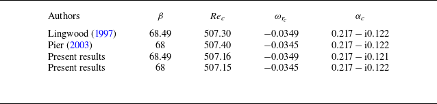
Starting from the identified saddle point, the variation of the absolute complex frequency and complex wavenumber is tracked along the streamwise direction. The values at other streamwise locations can be initially estimated by extrapolation and then quickly converged to precise values using the iterative method, ultimately yielding the distribution of the absolute growth rate along the streamwise direction. It is important to note that, during the tracking process, the dominant saddle point at the current location may become invalid at subsequent locations. When encountering a sudden change in the growth rate curve, it is necessary to recalculate the ‘global mode map’ at that location, find the new valid saddle point, and continue iteratively tracking the valid saddle points downstream using this as the new starting point. Based on the above discussion, the absolute instability characteristics of the boundary layer corresponding to different azimuthal wavenumbers can be easily identified. Table 2 provides the critical parameters for the onset of absolute instability in the von Kármán boundary layer as reported in classical studies (Lingwood Reference Lingwood1997; Pier Reference Pier2003). Whether
 $\beta =68.49$
or
 $68$
, the critical real frequency
 $\omega _{r_c}$
and the critical radial wavenumber
 $\alpha _c$
obtained in the present results are extremely close to those reported in the classical literature. This demonstrates that the current method achieves a sufficiently high level of accuracy in capturing the critical Reynolds number for absolute instability.
Critical values for the onset of absolute instability in the von Kármán boundary layer.

4. Results of local linear instability analysis
The Chebyshev spectral method offers a significant advantage in directly solving for all eigenmodes under specific parameters. Figure 5 illustrates the eigenvalue spectra
 $(\alpha _r, -\alpha _i)$
obtained for spatial mode analysis at
 $\beta =45$
and
 $\omega =0$
at
 ${\textit{Re}}=200, 250, 300, 350, 400, 450, 500$
and
 $550$
. Three distinct groups of eigenmodes are highlighted in the figure. Among them, the type III mode is characterised by a large radial growth rate
 $-\alpha _i$
but has a negative group velocity, leading to its designation as an ‘upstream mode’. In the von Kármán boundary layer, this mode represents the key branch responsible for the occurrence of absolute instability, as shown in figure 4. The type I and type II modes also appear in the von Kármán boundary layer. Lingwood (Reference Lingwood1995) demonstrated through inviscid and viscous analyses that the type I mode is independent of viscosity and arises from the inflection point of the radial velocity profile, representing an inviscid crossflow instability. Meanwhile, the type II mode is absent in inviscid analysis and instead reflects a subtle balance between viscous and Coriolis forces. Together, these three groups of modes reveal the underlying instability characteristics of the boundary layer. It should be emphasised that the naming of these modes is based solely on the chronological order of their discovery in the von Kármán boundary layer and does not imply any additional physical significance.
The eigenvalue spectra
 $(\alpha _r, -\alpha _i)$
obtained under spatial mode analysis for
 $\beta =45$
and
 $\omega =0$
at Reynolds numbers
 ${\textit{Re}}=200, 250, 300, 350, 400, 450, 500, 550$
.

Neutral (
 $\omega _i= 0, \alpha _i= 0$
) stability diagrams for stationary modes.

By setting the frequency
 $\omega =0$
, the convective instability characteristics of the stationary modes can be investigated through the stability analysis of the spatial mode. Figure 6 presents the neutral stability diagrams (
 $\omega _i= 0, \alpha _i= 0$
) of the stationary modes in the
 $({\textit{Re}}-\beta )$
and
 $({\textit{Re}}-\alpha )$
planes. The earliest critical Reynolds number for the onset of instability is found to be
 ${\textit{Re}}_c = 204.0$
, corresponding to the azimuthal wavenumber
 $\beta =27$
. Interestingly, when
 $\beta \leqslant 25$
, the neutral curve indicates that all stationary modes are stable, with
 $\omega _i\lt 0$
. Despite the significance of these findings, it is important to note that currently there is a lack of high-precision experimental data on the rotating-disk boundary layer in the rotor–stator cavity, which could provide valuable insights into the behaviour and characteristics of stationary modes. Interestingly, fluctuations in the neutral curve are observed near
 ${\textit{Re}}=330$
in our results, as highlighted by red circles in figure 6(
 $a$
). A similar phenomenon was reported by Lingwood (Reference Lingwood1995) in the von Kármán boundary layer through inviscid analysis. Their study further demonstrated that these fluctuations vanish when viscosity is neglected (see their figure 2). Consequently, they divided the neutral curve into two branches: branch 1 and branch 2, with the fluctuation region marking the transition between them. Branch 1, which is independent of viscosity, was identified as an inviscid instability caused primarily by the inflection point of the radial velocity profile. After introducing viscosity, significant changes were observed in the lower branch of the neutral curve beyond the fluctuation region at higher Reynolds numbers. This portion of the neutral curve was identified as branch 2, where viscous effects dominate (Alfredsson et al. Reference Alfredsson, Kato and Lingwood2024).
(
 $a$
) Variation of the two spatial modes with the largest radial growth rates,
 $-\alpha _i$
, as a function of
 ${\textit{Re}}$
under the condition
 $\omega = 0$
. (
 $b$
) The two modes with the largest growth rates exhibit a crossing. In this schematic, at the crossing point
 ${\textit{Re}}$
, the eigenvector
 $\hat {\boldsymbol{q}}$
corresponding to the larger
 $-\alpha _i$
is labelled as
 $a$
, while the eigenvector corresponding to the smaller
 $-\alpha _i$
is labelled as
 $A$
. By incrementally varying the Reynolds number with a step size
 $\Delta {\textit{Re}} = 1$
, the corresponding eigenvectors are defined as the letters shown in the figure.

To investigate whether the observed fluctuations are governed by the same instability mechanisms as those in the von Kármán boundary layer, particularly in terms of the transition between different instability modes, the specific
 $\beta$
are chosen. Using spatial mode analysis, the variations of the maximum growth rates
 $-\alpha _i$
for the two leading modes were computed as functions of
 ${\textit{Re}}$
, as shown in figure 7(
 $a$
). For each combination of
 ${\textit{Re}}$
and
 $\beta$
, the largest growth rate
 $-\alpha _i$
determines the stability of the system. The upper-left portion of the figure depicts the transition of
 $-\alpha _i$
from negative to positive, representing the shift of the disturbance from a stable to an unstable state. However, as
 ${\textit{Re}}$
increases further, all
 $-\alpha _i$
values become negative, indicating a return to stability. The continuous variation of the radial growth rates
 $-\alpha _i$
with
 ${\textit{Re}}$
results in the two curves for each wavenumber being connected based solely on the magnitude of
 $-\alpha _i$
. Current results indicate that the left side of the minimum of the curve with the larger
 $-\alpha _i$
corresponds to the inviscid type I mode, while the left side of the maximum of the curve with the smaller
 $-\alpha _i$
corresponds to the viscous type II mode. The classification of the right-hand portions of these curves, however, remains ambiguous. A notable feature occurs for
 $\beta =26-28$
, where the minima and maxima of the two curves approach each other at certain
 ${\textit{Re}}$
. For
 $\beta =28.5$
and
 $29$
, despite refining the Reynolds number interval
 $\Delta {\textit{Re}}$
, the two curves remain distinctly separated.
To further elucidate the nature of the modes near the extrema of the same curve, a detailed examination of the eigenvectors associated with different eigenvalues was conducted. Figure 7(
 $b$
) outlines the methodology: for each
 $\beta$
, the eigenvector corresponding to the minimum of the curve with the larger
 $-\alpha _i$
is designated as
 $a$
, while the maximum of the curve with the smaller
 $-\alpha _i$
is designated as
 $A$
. Eight additional eigenvectors were extracted at uniform intervals of
 $\Delta {\textit{Re}}=1$
. Following the methodology proposed by Oberleithner et al. (Reference Oberleithner, Sieber, Nayeri, Paschereit, Petz, Hege, Noack and Wygnanski2011), the dot products between these ten eigenvectors were computed. Eigenvectors yielding dot products close to 1 were identified as belonging to the same mode, providing a robust criterion for distinguishing mode types.
Table 3 provides a detailed summary of the dot product computations, where
 ${ab} = \hat {\boldsymbol{q}}_a^{H} \hat {\boldsymbol{q}}_b$
. All other terms are computed using the same methodology. It can be definitively concluded that
 $a$
and
 $A$
do not belong to the same mode, establishing
 $aA$
as a reliable threshold: only when the dot product exceeds
 $aA$
can it be asserted that the corresponding eigenvector sets belong to the same mode. For
 $\beta =26.5, 27, 27.5, 28.5$
and
 $29$
, the results in bold show deviations from 1 of less than 0.0001, allowing for precise identification of modes belonging to the same group. In the case of
 $\beta =26.5, 27$
and
 $27.5$
, the two mode groups exhibit intersections. To the left of the intersection point, the stability characteristics are dominated by the type I mode, whereas to the right, the type II mode becomes dominant. For
 $\beta =28.5$
and
 $29$
, no intersections are observed, and the stability characteristics remain consistently governed by the type I mode. For
 $\beta =28$
, the four largest dot products suggest a preliminary indication of mode intersections. However, for
 $\beta =28.1$
and
 $28.2$
, it becomes evident that the two mode groups no longer intersect, suggesting that for
 $\beta \leqslant 28$
, the dominant instability mechanism transitions.
The dot product between various eigenvectors for selected representative wavenumbers, as illustrated in Figure 7(
 $b$
), is computed as
 ${ab} = \hat {\boldsymbol{q}}_a^{H} \hat {\boldsymbol{q}}_b$
. The values highlighted in bold denote the four largest entries among the eight results, which are also the closest to 1, signifying a high degree of similarity between the corresponding eigenvectors.

At
 $\beta =28$
, the maximum radial growth rate of the type II mode is
 $-\alpha _i = -0.000127 \lt 0$
, confirming that, in the current rotating-disk boundary layer, the type II mode has never governed the stability of the stationary mode (
 $\omega =0$
). Thus, the fluctuations in the neutral curve depicted in figure 6 cannot be attributed to a transition between dominant modes but rather represent an intrinsic property of the type I mode. This implies that the neutral curve is governed solely by a single branch.
In the von Kármán boundary layer, the upstream modes intersect with the inviscid crossflow modes at specific
 ${\textit{Re}}$
and azimuthal wavenumbers
 $\beta$
, resulting in the formation of a saddle point and the emergence of absolute instability (Lingwood Reference Lingwood1995). As shown in figure 5, the existence of upstream modes and crossflow modes has been identified in the rotating-disk boundary layer. Therefore, the next logical step is to examine the evolution of these modes as a function of
 ${\textit{Re}}$
. Figure 8 illustrates the variation of the radial wavenumber
 $\alpha$
with Reynolds number
 ${\textit{Re}}$
for three instability modes in the rotating-disk boundary layer under spatial mode analysis, with parameters set to
 $\beta =45$
and
 $\omega =0$
. These represent stationary disturbances relative to the rotating disk. The Reynolds number range for the type I and type II modes is
 ${\textit{Re}} \geqslant 150$
, while the type III mode appears only when
 ${\textit{Re}} \geqslant 235$
. For the type I and type II modes, data with
 ${\textit{Re}} \geqslant 150$
are sufficient to capture their characteristics. However, the type III mode is absent for
 ${\textit{Re}} \lt 235$
, as spatial stability analysis does not identify its presence at lower Reynolds numbers. For the type I and type II modes, the real part of the radial wavenumber,
 $\alpha _r$
, decreases as
 ${\textit{Re}}$
increases. In contrast,
 $\alpha _r$
for the type III mode increases with
 ${\textit{Re}}$
and asymptotically approaches
 $\alpha _r = 0.21$
. For the Reynolds number
 ${\textit{Re}} \gt 250$
, the radial growth rate of the type I mode is greater than 0, and it is the fastest developing mode along the streamwise direction in the boundary layer. In contrast, the radial growth rate of the type II circular wave mode is always less than 0, implying that circular wave instability will not occur. Although figure 8(
 $b$
) shows a trend of mutual approach between the type I and type III modes, the study by Lingwood (Reference Lingwood1995) on the absolute instability of the von Kármán boundary layer reveals that stationary modes do not exhibit absolute instability.
Radial wavenumber
 $\alpha$
for disturbances of the normal mode form for
 $\beta = 45$
and
 $\omega = 0$
.

Furthermore, through the space-temporal mode stability analysis method described in the previous section, the absolute instability of the rotating-disk boundary layer was discovered. At
 ${\textit{Re}}=409.6$
and
 $\beta =85$
, absolute instability first appears. The absolute frequency is found to be
 $\omega _{r_c} = -0.038617$
. By taking this complex frequency as the global complex frequency of the spatial mode, the evolution of the radial growth rate
 $-\alpha _i$
of type I and type III modes with respect to the Reynolds number
 ${\textit{Re}}$
can be obtained, as illustrated in figure 9. If the rotating-disk boundary layer exhibits global linear instability with a global frequency of
 $\omega _{r_c} = -0.038617$
, then this figure suggests that the wavemaker of the global instability is located at
 ${\textit{Re}}=409.6$
. The left portion of the type III modes, labelled as
 $\alpha _i^-$
, represents the radial growth rate of the upstream mode, which is also the radial growth rate of the global linear mode. In contrast, the left portion of the type I modes, labelled as
 $\alpha _i^+$
, corresponds to the radial growth rate of the convective instability mode (if it exists). This information will be further discussed in the following text. Figure 10 illustrates the disturbance velocity distribution of the type I mode corresponding to
 ${\textit{Re}}=409.6, \beta =85$
and
 $\omega _{r_c} = -0.038617$
. The disturbance velocity components
 $\widetilde u, \widetilde v$
and
 $\widetilde w$
have been normalised using
 $\mathrm{{max}}(\widetilde v)$
. For the azimuthal disturbance velocity
 $\widetilde v$
, the peak value is observed at
 $z_\delta =0.997$
. In contrast, for the von Kármán boundary layer, the peak value of the azimuthal disturbance velocity is located at
 $z_\delta =1.3$
.
Under the local linear stability analysis of the spatial mode, the evolution of the radial growth rate
 $-\alpha _i$
of type I and type III modes with respect to the Reynolds number
 ${\textit{Re}}$
, given
 $\omega _{r_c} = -0.038617$
.

The disturbance velocity distribution of the type I mode corresponding to
 ${\textit{Re}}=409.6,\beta =85$
and
 $\omega _r = -0.038617$
.

Absolute instability of the rotating-disk boundary layer. (
 $a$
) Neutral (
 $\omega _i= 0, \partial \omega /\partial \alpha = 0$
) stability diagrams for absolute instability, (
 $b$
) Variation of the complex frequency
 $\omega = \omega _r + \mathrm{i}\omega _i$
of absolute instability with the Reynolds number
 ${\textit{Re}}$
for
 $\beta = 85$
.

Figure 11(
 $a$
) presents the neutral curve of the absolute instability in the rotating-disk boundary layer. The critical Reynolds number for the onset of absolute instability is found to be
 ${\textit{Re}}_{c}=409.6$
, with a corresponding azimuthal wavenumber of
 $\beta =85$
. In contrast, for the von Kármán boundary layer, absolute instability first emerges at
 ${\textit{Re}}=507.3$
with an azimuthal wavenumber of
 $\beta =68$
. However, it is important to note that this does not necessarily imply that the rotating-disk boundary layer is more unstable than the von Kármán boundary layer. When considering the viscous scale
 $\delta _d^*=\sqrt {\nu ^*/\varOmega _d^*}$
, which is based on the angular velocity of the disk
 $\varOmega _d^*$
, the absolute instability in the rotating-disk boundary layer occurs at
 $r^*=570.3\delta _d^*$
, which is greater than the corresponding value of
 $507.3\delta _d^*$
for the von Kármán boundary layer. This location corresponds to a local rotational Reynolds number of
 ${\textit{Re}}_r = \varOmega ^*_dr^{*2}/\nu ^* \approx 3.42\times 10^5$
.
Figure 11(
 $b$
) presents the absolute complex frequency
 $\omega =\omega _r+\mathrm{i}\omega _i$
for the special azimuthal wavenumber
 $\beta =85$
under different local Reynolds numbers
 ${\textit{Re}}$
, as it is the earliest wavenumber to exhibit absolute instability. The black line in the figure denotes the temporal growth rate
 $\omega _i$
, while the grey line represents the temporal frequency
 $\omega _r$
. At
 ${\textit{Re}}=409.6$
,
 $\omega _i$
begins to exceed 0, gradually increasing and reaching a maximum at
 ${\textit{Re}}=648$
. For
 ${\textit{Re}} \gt 1168$
,
 $\omega _i\lt 0$
, indicating the disappearance of absolute instability. This trend aligns with the findings of Davies et al. (Reference Davies, Thomas and Carpenter2007) regarding the von Kármán boundary layer. The temporal frequency
 $\omega _r$
of both boundary layer instability modes exhibit a gradual increase from negative to positive values, suggesting that the azimuthal migration speed of the instability modes transitions from being slower to faster than the disk rotation speed. Crucially, if a global linear instability is present for
 $\beta =85$
, the corresponding global frequency can be determined from this figure (Healey Reference Healey2010). To optimise computational resources, subsequent investigations into global linear instability solely consider the instability mode of
 $\beta =85$
. Similarly, studies by Appelquist et al. (Reference Appelquist, Schlatter, Alfredsson and Lingwood2015, Reference Appelquist, Schlatter, Alfredsson and Lingwood2016b
), Lee et al. (Reference Lee, Nishio, Izawa and Fukunishi2018) selected the azimuthal wavenumber
 $\beta =68$
, which is the first to display absolute instability in the von Kármán boundary layer. Experimental measurements by Imayama et al. (Reference Imayama, Alfredsson and Lingwood2013, Reference Imayama, Alfredsson and Lingwood2014) successfully captured the dominant azimuthal wavenumber
 $\beta =68$
.
5. Method of numerical simulation
The global stability analysis is conducted using the open-source solver Nek5000 (Fischer, Lottes & Kerkemeier Reference Fischer, Lottes and Kerkemeier2012), which employs a spectral element method based on Legendre polynomials to solve the incompressible N–S equations. To achieve optimal polynomial-order-based refinement within the spectral elements, seventh-order polynomials are utilised for each spectral element, striking a balance between resolution and computation time. The spatial discretisation adopts the standard
 $P_N-P_{N-2}$
method, where velocity is defined at each Gauss–Lobatto–Legendre (GLL) point, while pressure is solely defined at Gauss–Legendre points. This approach effectively eliminates spurious pressure modes. The Nek5000’s temporal discretisation scheme is based on operator splitting, with the nonlinear convective terms treated explicitly via an extrapolation scheme (EXT) and the viscous and divergence operators treated implicitly. The implicit scheme employs the backward differential formula, and a second-order scheme is consistently selected for all global linear simulations (Karniadakis, Israeli & Orszag Reference Karniadakis, Israeli and Orszag1991). This combination of spatial and temporal discretisation techniques ensures accurate and efficient computation of the global stability characteristics.
5.1. Governing equations
Nek5000 is capable of solving the complete incompressible N–S equations:
 \begin{align} \frac {{\partial {\boldsymbol{U_x}}}}{{\partial t}} + {\boldsymbol{U_x}} \boldsymbol{\cdot }\boldsymbol{\nabla }{\boldsymbol{U_x}} =& - \boldsymbol{\nabla }p + \frac {|Ro|}{{\textit{Re}}_d}\sqrt {\frac {\varOmega }{\varOmega _d}}{\boldsymbol{\nabla} ^2}{\boldsymbol{U_x}} + \boldsymbol{f_x}, \end{align}
 \begin{align}& \boldsymbol{\nabla }\boldsymbol{\cdot }\boldsymbol{U_x} = 0. \end{align}
Here
 $\boldsymbol{U_x} = (U_x,U_y,W)$
represents the velocity distribution in the Cartesian coordinate system and
 ${\textit{Re}}_d$
denotes the Reynolds number of the maximum non-dimensional radial position of the computational domain (
 ${\textit{Re}}_d = r_d^*|Ro|/\delta ^*$
). In our study the nonlinear numerical simulations are implemented by directly solving the complete incompressible N–S equations. Meanwhile, within the global linear stability framework, the laminar self-similar velocity profile
 $\boldsymbol{U_x}$
is preserved as the base flow, upon which a perturbation field
 $\boldsymbol{u_x}$
is superimposed. The focus is then directed toward solving the linearised N–S equations governing the perturbation dynamics:
 \begin{align} \frac {{\partial {\boldsymbol{u_x}}}}{{\partial t}} + {\boldsymbol{U_x}} \boldsymbol{\cdot }\boldsymbol{\nabla }{\boldsymbol{u_x}} +{\boldsymbol{u_x}} \boldsymbol{\cdot }\boldsymbol{\nabla }{\boldsymbol{U_x}} = &- \boldsymbol{\nabla }p + \frac {|Ro|}{{\textit{Re}}_d}\sqrt {\frac {\varOmega }{\varOmega _d}}{\boldsymbol{\nabla} ^2}{\boldsymbol{u_x}} + \boldsymbol{f_x}, \end{align}
 \begin{align} \boldsymbol{\nabla }\boldsymbol{\cdot }\boldsymbol{u_x} &= 0. \end{align}
Here
 $p$
represents pressure,
 $t$
denotes time and a forcing term
 $\boldsymbol{f_x}$
is employed to impose initial perturbations and sponge layers at the inlet and outlet. In the governing equations, the length scale is non-dimensionalised using the viscous scale
 $\delta ^*_d$
based on the angular velocity
 $\varOmega _d^*$
of the rotating disk, the time scale is non-dimensionalised using
 $1/\varOmega _d^*$
, the pressure term is non-dimensionalised using
 $\rho (\varOmega _d^* \delta ^*_d)^2$
and the velocity is non-dimensionalised using
 $\varOmega _d^* \delta ^*_d$
. The rotation number of the disk is defined as
 $T = t\varOmega _d^*/(2\unicode {x03C0})$
. In the simulations,
 $\varOmega _d^*=1$
is used, resulting in
 $T = t/(2\unicode {x03C0})$
. It is important to note that in the local linear stability analysis, the length scale is non-dimensionalised using the viscous scale
 $\delta ^*$
based on the system rotation speed
 $\varOmega ^*$
. Furthermore, the non-dimensionalisation methods for time, velocity and pressure differ between the local and global analyses. To obtain valid results in subsequent analyses, it is crucial to convert them to a consistent non-dimensionalisation scheme. It should be noted that Nek5000 is based on the Cartesian coordinate system
 $(x, y, z)$
, whereas the laminar self-similar solution on the rotating disk is obtained within the cylindrical coordinate system
 $(r, \theta , z)$
. To reconcile these coordinate systems, the laminar self-similar solution
 $({U}, {V}, {W})$
is first transformed into the Cartesian coordinate system as
 $({U_x}, {U_y}, {W})$
before the simulation begins. After the simulation, the results
 $({U_x}, {U_y}, {W})$
are transformed back into the cylindrical coordinate system for detailed analysis and further processing.
5.2. Mesh
The global linear and direct numerical simulations are defined within an annular sector of size
 $2\unicode {x03C0}/85$
rad. The spectral element grid nodes are initially defined in cylindrical coordinates and then mapped to the Cartesian coordinate system using high-order polynomials at the commencement of the simulation.
In a manner consistent with local linear stability analysis, the computational domain is truncated outside the rotating-disk boundary layer to mitigate the influence of the stationary-disk boundary layer, while also accounting for radial boundary conditions. Figure 12(
 $a$
) illustrates this concept. At
 ${\textit{Re}}_h=2000$
, the rotating disk is located at
 $z=0$
and the stationary disk at
 $z=89.4$
. For the simulation, only the pink-shaded region is considered as the computational domain, with all other regions excluded. Figures 12(
 $b$
), 12(
 $c$
) and 12(
 $d$
) detail the computational domains for the global linear simulation L5 and the DNS NL1 and NL2, respectively. The radial coordinate
 $r^*$
and the axial coordinate
 $z^*$
are non-dimensionalised as
 $r = r^*/\sqrt {\nu ^*/\varOmega ^*_d},z = z^*/\sqrt {\nu ^*/\varOmega ^*_d}$
, respectively.
Meridional plane
 $(r, z)$
schematic of the computational model. (
 $a$
) The computational domain model includes a rotating disk and a stationary disk. At
 ${\textit{Re}}_h=2000$
, the rotating disk is located at
 $z=0$
and the stationary disk at
 $z=89.4$
. To avoid the influence of the stationary-disk side, only the pink region is selected as the computational domain for the simulation. (
 $b$
) Computational domain for global linear simulation L5. The boundary condition
 $v$
is Dirichlet, and ON indicates a mixture of both Dirichlet and homogeneous Neumann boundary conditions. The axial computational domain extends over
 $0 \leqslant z \leqslant 20$
. (
 $c$
) Computational domain for DNS NL1, the axial computational domain extends over
 $0 \leqslant z \leqslant 49.3$
. (
 $d$
) Computational domain for DNS NL2, where SYM represents a symmetry condition. The grey shaded region indicates the smooth growth area of the sponge function, while the black shaded region indicates the area where the sponge function has reached its maximum value.

For the linear numerical simulation, the radial computational domain extends from
 $r = 400$
to
 $r = r_d$
, with spectral element nodes uniformly spaced at intervals of
 $\Delta r = 2$
. The azimuthal resolution, in this case, is specified by an interval of
 $\Delta \theta = 2\unicode {x03C0}/(85\times 11)$
. The maximum radial position is
 $r_d=840$
, resulting in the ratio of the azimuthal spectral element interval to the radial spectral element interval in the Cartesian coordinate system,
 $r\Delta \theta /\Delta r$
, gradually increasing from 1.34 to 2.82. In the normal direction of the boundary layer, the spectral element grid nodes follow an exponentially growing strategy, i.e.
 \begin{equation} {z_n} = \sum \limits _{i = 1}^n {\Delta z{a^{i - 1}}}, \end{equation}
where
 $z_n$
is the coordinate position of the
 $n$
th normal node,
 $\Delta z$
is the interval of the first layer of the normal grid and
 $a$
is the stretching factor. We set
 $\Delta z=0.223$
and
 $a=1.15$
, which correspond to the number of normal spectral elements
 $n=19$
and the maximum position
 $z_{\textit{max}}=20$
. Appelquist et al. (Reference Appelquist, Schlatter, Alfredsson and Lingwood2015) also employed a similar normal grid distribution to conduct linear simulations of the von Kármán boundary layer. However, the radial spectral element grid spacing in the current study is half of that used in Appelquist et al. (Reference Appelquist, Schlatter, Alfredsson and Lingwood2015). We also performed simulations using
 $\Delta r = 4$
, but for smaller perturbations in the linear region, this grid could only capture magnitudes of
 $10^{-8}$
, whereas the results obtained with
 $\Delta r = 2$
could capture magnitudes of
 $10^{-14}$
. Consequently,
 $\Delta r = 2$
was selected for all studies to ensure accurate resolution of the perturbations.
For the DNS, the radial computational domain is defined from
 $r = 500$
to
 $r = 900$
, with spectral element nodes uniformly distributed at an interval of
 $\Delta r \leqslant 2$
. In the NL2 configuration, significant changes in the flow field were detected near
 $r = 820$
, which necessitated localised radial refinement to better capture the flow dynamics in this region. The azimuthal resolution is characterised by a grid interval of
 $\Delta \theta = 2\unicode {x03C0}/(85 \times 31)$
. In the normal direction of the boundary layer, the grid parameters are configured as
 $\Delta z = 0.4$
and
 $a = 1.08$
, yielding 31 normal spectral elements (
 $n = 31$
) and a maximum position of
 $z_{\textit{max}} = 49.3$
.
The details of the spectral element grid for all cases are provided in table 4, where L1–L8 represent the linear simulation and NL1 and NL2 represent the DNS in this study. The radial outer boundary of the domain is indicated by
 $r_d$
, and a sponge layer is applied at the outer boundary starting from
 $r_s$
. Meanwhile,
 $r_{\textit{ex}}$
represents the radial position at which the initial impulsive disturbance is introduced into the system. These represent special radial positions in the numerical simulations. However, in the actual analysis of this study, the Reynolds number
 ${\textit{Re}}$
from the BEK model is employed to represent the radial position, involving the transformation
 ${\textit{Re}}=r|Ro|\sqrt {\varOmega /\varOmega _d}$
. The table presents
 ${\textit{Re}}_d$
,
 ${\textit{Re}}_s$
and
 ${\textit{Re}}_{\textit{ex}}$
, which correspond to the radial Reynolds numbers of
 $r_d$
,
 $r_s$
and
 $r_{\textit{ex}}$
, respectively. It is important to note that
 ${\textit{Re}}_{\textit{end}}$
, representing the location of the end of the linear domain in this study, is a position that can only be determined through subsequent analysis and will be further elaborated on later. Here
 $N_r$
and
 $N_{nel}$
represent the number of spectral elements in the radial direction and the total number of spectral elements in the simulation, respectively.
Summary of the parameters for the linear simulations. Here L1–L8 represent the linear simulations and NL1 and NL2 represent the DNS in this study. The radial outer boundary of the domain is indicated by
 $r_d$
, and a sponge layer is applied at the outer boundary starting from
 $r_s$
,
 ${\textit{Re}}_d$
and
 ${\textit{Re}}_s$
are the Reynolds numbers corresponding to
 $r_d$
and
 $r_s$
, respectively. Here
 ${\textit{Re}}_{\textit{end}}$
represents the end of the linear region, while
 $r_{\textit{ex}}$
denotes the radial location of the initial impulsive disturbance,
 ${\textit{Re}}_{\textit{ex}}$
is the Reynolds numbers corresponding to
 $r_{\textit{ex}}$
;
 $N_r$
and
 $N_{nel}$
represent the number of spectral elements in the radial direction and the total number of spectral elements in the simulation, respectively.

While the Nek5000 solver generates the final velocity distribution in the Cartesian coordinate system, the physical nature of the current problem is better represented by analysing the space and flow field in the cylindrical coordinate system during post-processing. To achieve this, all monitoring point results and complete three-dimensional flow field data in this study are interpolated onto a denser, uniformly distributed grid with increments of
 $\Delta r$
and
 $\Delta \theta$
. Within each spectral element, Legendre polynomials are computed at the GLL quadrature points, and the solution is expressed as the sum of these polynomials. Consequently, spectral interpolation can be applied to obtain the solution at any spatial location without compromising accuracy. The simulation data are saved 349 times during each rotation of the disk.
5.3. Boundary conditions
The fundamental concept behind the boundary conditions is to apply a sponge function at the radial boundary to damp all perturbations. This allows the flow to revert to the laminar self-similar solution of the rotating-disk boundary layer, effectively preventing downstream perturbations from reflecting off the outflow boundary. The sponge function takes the form
 \begin{equation} \boldsymbol{f_x} = -\lambda (r) \boldsymbol{u_x}, \end{equation}
where the function
 $\lambda (r)$
is given by
 \begin{equation} \lambda (r) = \begin{cases} 1 & (r \leqslant 410), \\[6pt] 1 - 1/\left(1 + {\mathrm e}^{1/(r_1-1)+1/r_1}\right) & (410 \lt r \lt 420) \left ( r_1 = \dfrac {r-410}{10} \right )\!, \\[6pt] 0 & ({420} \leqslant r \leqslant r_s), \\[6pt] 28/\left(1 + {\mathrm e}^{ 1/(r_2-1)+1/r_2}\right) & \left(r_s \lt r \lt r_s+40\right) \left ( r_2 = \dfrac {r-r_s}{40} \right )\!, \\[6pt] 28 & (r \geqslant r_s+40). \end{cases} \end{equation}
The scope of the effect of this formula corresponds to the grey and black shaded regions in figure 12. All cases in the study employ an identical sponge layer at the inlet. The purpose of this inflow sponge is to damp low-amplitude upstream propagating waves, which have the potential to be reflected at the inner radial boundary.
For the global linear simulations (L1–L5, L8), the outlet sponge layer is defined by setting
 $r_s = r_d - 100$
, ensuring a uniform sponge layer configuration near the outlet. Conversely, in cases L6 and L7, the values of
 $r_s$
are adjusted to
 $r_d - 80$
and
 $r_d - 60$
, respectively, to examine how variations in sponge layer shape influence the linear simulation region. Despite these modifications, the smooth transition phase of the sponge layer is maintained across all cases. For linear numerical simulations, the coefficient 28 is used as the amplification factor for the sponge layer. Boundary conditions are carefully specified for the top and bottom boundaries of the computational domain. In figure 12(
 $b$
), at the bottom boundary corresponding to the rotating-disk surface (
 $z = 0$
), the perturbation components
 $\boldsymbol{u_x} = (u_x, u_y, w)$
are set to zero, enforcing a no-slip condition. At the top boundary (
 $z = 20$
), a combination of Dirichlet and stress-free Neumann conditions is applied. Specifically, the radial and azimuthal perturbation velocities,
 $u_x$
and
 $u_y$
, are set to zero, while the wall-normal velocity
 $w$
satisfies the stress-free Neumann condition
 $\mathrm{d}w/\mathrm{d}z = p$
. This condition allows the flow to freely adjust in the wall-normal direction while ensuring zero shear stress.
For the DNS NL1, the outlet sponge layer is defined by setting
 $r_s = r_d - 80$
, but the sponge layer coefficient is modified to 10. It should be noted that since the numerical simulation computes the instantaneous flow field
 $\boldsymbol{U_x} = (U_x, U_y, W)$
, additional computations are required at every time step to ensure that the flow field within the sponge layer returns to the velocity profile of the laminar self-similar solution. This is achieved by calculating
 $\boldsymbol{u_x} = \boldsymbol{U_x} - \boldsymbol{U}_{\boldsymbol{x}, l}$
, where
 $\boldsymbol{U}_{\boldsymbol{x}, l}$
represents the laminar self-similar solution of the rotating-disk boundary layer expressed in the Cartesian coordinate system. For the NL2 case, the bottom boundary condition within the range
 $820 \leqslant r \leqslant 900$
is modified to SYM, a symmetry condition. Additionally, a sponge layer is applied in the range
 $885 \leqslant r \leqslant 900$
, but its purpose is not to restore the flow field to the laminar self-similar velocity profile. Instead, it enforces zero azimuthal and axial velocities while imposing no additional restrictions on the radial velocity. Consequently, (5.6) is no longer valid in this scenario. The objective of this set-up is to create a boundary condition similar to a radial boundary of the rotating disk at
 $r = 820$
, which is a radial jet boundary condition. This configuration allows for the investigation of how different radial boundary conditions influence global nonlinear behaviour. It is worth noting that the sponge layer functions described above have been successfully employed in the study conducted by Appelquist et al. (Reference Appelquist, Schlatter, Alfredsson and Lingwood2015, Reference Appelquist, Schlatter, Alfredsson and Lingwood2016b
, Reference Appelquist, Schlatter, Alfredsson and Lingwood2018). In the stationary reference frame, the pressure
 $P$
increases continuously along the radial direction
 $r$
due to centrifugal effects. To simplify the implementation of the boundary condition
 $\mathrm{d}W/\mathrm{d}z=P$
at the top boundary, the DNS is carried out in a reference frame rotating with the angular velocity
 $\varOmega _{\!f}$
of the core region, where the pressure
 $P$
remains constant. However, this adjustment requires that the corresponding initial flow field and the precise velocity boundary conditions in the nonlinear simulations subtract the corresponding rotational velocity
 $\varOmega _{\!f} r$
. Similarly, the Coriolis force term
 $-2\boldsymbol{\varOmega _{\!f}} \times \boldsymbol{U_x}$
needs to be introduced into the equations, where
 $\boldsymbol{\varOmega _{\!f}} = (0, 0, \varOmega _{\!f})$
.
At both ends of the computational sector, the rotational symmetry boundary conditions readily available in the Nek5000 solver are utilised, the details of which are omitted for brevity.
5.4. Initial conditions
To investigate the response of the rotating-disk boundary layer to an instantaneous pulse perturbation, an initial perturbation is introduced through a body force applied at the rotating-disk surface. The body force is composed of four variables, with Gaussian shape functions introduced in both the radial
 $r$
direction and the axial
 $z$
direction, a sinusoidal function in the azimuthal
 $\theta$
direction, and a rapid growth followed by decay in the time direction. The body force is expressed as
 \begin{equation} \boldsymbol{f_x}=-{a_{\!f}}[a(r) \boldsymbol{\cdot }b(z) \boldsymbol{\cdot }c(t) \boldsymbol{\cdot }d(t,\theta )](\boldsymbol{U_x-U_d}), \end{equation}
where
 $a(r) \boldsymbol{\cdot }b(z) \boldsymbol{\cdot }c(t) \boldsymbol{\cdot }d(t,\theta )$
effectively specifies the spatial and temporal coefficients of the forcing;
 $a_{\!f}$
represents the scaling factor of the initial excitation;
 $\boldsymbol{U_x}$
represents the spatial distribution of the velocity field in the rotating-disk boundary layer during the simulation, while
 $\boldsymbol{U}_{\!d}$
denotes the velocity of the rotating disk at the corresponding radial position
 $r$
. The individual components of the forcing are defined as follows:
 \begin{align} a(r) &= \mathrm{e}^{ -\lambda (r-r_{\textit{ex}})^{ 2}}\mathrm{e}^{\mathrm{i} \alpha (r-r_{\textit{ex}})}, \end{align}
 \begin{align} b(z) &= \mathrm{e}^{-\mu (z-z_{\textit{ex}})^{ 2}}, \end{align}
 \begin{align} c(t) &= \big(1 - \mathrm{e}^{ -\sigma t^{\mathrm 2}}\big)\mathrm{e}^{ -\sigma t^{ 2}}, \end{align}
 \begin{align} d(\theta , t) &= \mathrm{e}^{\mathrm{i}[ \beta (\theta -\varOmega _d t)]}. \end{align}
The parameters
 $\lambda = 0.5,\mu = 25$
and
 $\sigma = 50$
control the extent of the forcing in the radial (
 $r$
), axial (
 $z$
) and time (
 $t$
) directions, respectively. Here
 $r_{\textit{ex}}$
and
 $z_{\textit{ex}}$
represent the locations of the excitation in the radial and axial directions, with
 $r_{\textit{ex}}$
provided in table 4 and
 $z_{\textit{ex}}=0$
corresponding to the disk surface. The radial wavenumber of the perturbation is set to
 $\alpha = 0.251$
, while the azimuthal wavenumber is chosen as
 $\beta =85$
.
For the linear numerical simulation, the simulation is performed in a stationary coordinate system, the excitation experiences a phase change over time
 $t$
, mimicking the effect of a roughness element fixed on the rotating-disk surface. To prevent the initial disturbance from becoming excessively large and causing the disturbed flow field to quickly grow to the double-precision limit, a scaling factor of
 $a_{\!f}=0.001$
is applied. The temporal evolution of the forcing is governed by a Gaussian function, which reaches its maximum at around
 $t\approx 0.118$
and subsequently decays. For
 $t\gt 0.4$
, the forcing term
 $c(t)$
is set to zero. The Courant–Friedrichs–Lewy (CFL) condition is a necessary condition for the stability of explicit time integration schemes, and maintaining a CFL number below 1 is crucial for numerical stability. To ensure the accuracy of the time integration, the time step is set to
 $\Delta t = 2 \times 10^{-4}$
, which ensures that the CFL number remains below 0.5.
For the DNS, scaling factor
 $a_{\!f}=20$
, the angular velocity
 $\varOmega _d$
should be adjusted to
 $\varOmega _d-\varOmega _{\!f}$
, but details of these transformations are not discussed here. At these simulations, the time step is further reduced to
 $\Delta t = 6 \times 10^{-5}$
. Although the CFL number fluctuates, its maximum value remains below 0.5.
6. Results of global linear instability analysis
The azimuthal velocity component plays a dominant role in the overall dynamics of the rotating-disk boundary layer flow. As illustrated in figure 10, the peak of the azimuthal velocity associated with the unstable mode is found to occur at
 $z_\delta =0.997$
. To investigate the space-temporal evolution of the disturbance, monitoring data are extracted from the (
 $r,\theta$
) plane corresponding to
 $z = z_\delta \sqrt {\varOmega _d/\varOmega }=1.04$
. The r.m.s. of the azimuthal velocity is defined as
 \begin{equation} V_{\textit{rms}}(r, z, t) = \left [\frac {85}{ 2\unicode {x03C0}} \int _0^{2\unicode {x03C0} /85} \left (\frac {v(r, z, t)}{r}\right )^2 \mathrm{d}\theta \right ]^{0.5}. \end{equation}
Space–temporal diagram from L1 (
 $r_d=780, {\textit{Re}}_{d}=560.3$
) and L5 (
 $r_d=820, {\textit{Re}}_{d}=589.1$
); (
 $a$
)
 $\mathrm{log}_{10}(V_{\textit{rms}})$
from L1, (
 $b$
)
 $\mathrm{dln}(V_{\textit{rms}}(t))/\mathrm{d}t$
from L1, (
 $c$
)
 $\mathrm{log}_{10}(V_{\textit{rms}})$
from L5, (
 $d$
)
 $\mathrm{dln}(V_{\textit{rms}}(t))/\mathrm{d}t$
from L5.

Figure 13 illustrates the space–temporal evolution characteristics of the disturbances corresponding to the cases L1 (
 $r_d=780$
) and L5 (
 $r_d=820$
). The non-dimensional time
 $t/(2\unicode {x03C0})$
represents the number of revolutions of the disk, while the horizontal coordinate
 ${\textit{Re}}=r|Ro|\sqrt {\varOmega /\varOmega _d}$
denotes the Reynolds number used in the local linear stability analysis. In both cases, the disturbance excitation is introduced at a radial location of
 $r_{\textit{ex}}=600$
, corresponding to a Reynolds number of
 ${\textit{Re}} \approx 431.0 \gt 409.6$
, which lies within the absolute instability region. The black dashed line in the figure indicates the radial position that marks the beginning of the sponge layer. Figure 13(
 $a$
) employs a colour scale to represent the logarithm of the r.m.s. of the azimuthal velocity,
 $\mathrm{log}_{10}(V_{\textit{rms}})$
. The rapid decay of
 $V_{\textit{rms}}$
observed near the right edge of the figure can be attributed to the influence of the sponge layer. At
 $t=0$
, the disturbance begins to develop, and within an extremely short period (
 $t/(2\unicode {x03C0}) \lt 0.2$
), the leading edge of the wave packet reaches the outer edge of the radial boundary. In contrast, the trailing edge propagates downstream at a much slower rate. In the early stages, the disturbance exhibits primarily convective growth, advancing downstream slowly while increasing in amplitude. However, a distinct global growth rate is absent, as reflected by the misalignment of the contour lines, which are not inclined straight lines. Once
 $t/(2\unicode {x03C0}) \gt 2$
, the downstream propagation speed of the trailing edge stabilises, as indicated by the contour lines developing with a consistent inclination angle in the direction of increasing time and radial position (upper right in the figure). Additionally, all contour lines in the disturbance field evolve in a uniform direction, as denoted by the black arrows in the figure. This uniform evolution signifies that the disturbances have formed a global mode characterised by a constant temporal growth rate. Notably, this temporal growth rate is negative, indicating that the disturbances decay over time and eventually vanish, thereby rendering the boundary layer globally stable.
Figure 13(
 $b$
) provides further insight by illustrating the temporal growth rate of disturbances at various radial positions,
 $\mathrm{dln}(V_{\textit{rms}}(t))/\mathrm{d}t$
. The black solid line represents the zero-growth-rate contour,
 $\mathrm{dln}(V_{\textit{rms}}(t))/\mathrm{d}t=0$
. During the initial stages, excitation leads to a brief but rapid growth within the boundary layer, visualised as the bright red region in the figure, reflecting the characteristics of convective instability. For
 $t/(2\unicode {x03C0}) \gt 1.25$
, within the range
 $400 \lt {\textit{Re}} \lt 524$
, the temporal growth rate
 $\mathrm{dln}(V_{\textit{rms}}(t))/\mathrm{d}t$
becomes negative, indicating that disturbances at these radial positions will continue to decay until they completely vanish. It is worth noting that, for
 ${\textit{Re}} \lt 400$
, the amplitude of disturbances is exceedingly small, approaching the magnitude of numerical grid errors, and is therefore omitted from the figure. The simulation results presented are restricted to
 $t/(2\unicode {x03C0}) \lt 3$
, as the temporal growth rate’s rate of change has already decreased to less than
 $10^{-8}$
by this time. Thus, the subsequent spatiotemporal evolution of the flow field can be accurately inferred from the state at
 $t/(2\unicode {x03C0}) = 3$
, and further results are omitted.
When the radial computational domain is extended, the initial space-temporal development of instantaneous disturbances for L5 exhibits characteristics consistent with those of L1, showing pronounced convective instability. However, after
 $t/(2\unicode {x03C0}) \gt 2$
, the trailing edge of the wave packet ceases to propagate downstream and instead begins to move upstream in figure 13(
 $c$
). The contour lines of the entire disturbance field evolve in the direction indicated by the black arrows in the figure, providing preliminary evidence for the presence of a global linear instability mode. Figure 13(
 $d$
) further corroborates this global linear instability mode. In this figure, the black solid line (zero-growth-rate contour) exhibits a turning point at
 ${\textit{Re}} \approx 500$
, marking the transition from convective instability to absolute instability. As the absolute instability progressively contaminates the entire flow field, the black solid line evolves over time until reaching
 ${\textit{Re}}=400$
. The space-temporal domain shown in this figure matches that of figure 13(
 $b$
), as at
 $t/(2\unicode {x03C0}) = 3$
, the temporal growth rate’s rate of change has diminished to less than
 $10^{-8}$
. Therefore, it can be concluded that disturbances within the entire flow field will continue to grow linearly with time, affirming the existence of a global linear instability mode.
In the local linear simulations conducted by Davies & Carpenter (Reference Davies and Carpenter2003) for the von Kármán boundary layer (employing the parallel flow assumption for
 $r_a \gt 507.3$
), absolute instability rapidly emerges following the impulsive disturbance, aligning with the predictions derived from local linear stability analysis. The global linear study by Appelquist et al. (Reference Appelquist, Schlatter, Alfredsson and Lingwood2015) highlights that the establishment of global instability is intrinsically linked to the global frequency selection mechanism. Moreover, it is noted that linear global instability behaviour necessitates the triggering of upstream modes by the more unstable downstream regions. Viewed through this lens, both cases L1 and L5 successfully trigger upstream modes after a certain time, resulting in the emergence of a uniform global frequency throughout the flow field. However, a critical distinction arises in the fact that the global growth rate associated with the global frequency in L1 is less than 0, signifying global stability. Appelquist et al. (Reference Appelquist, Schlatter, Alfredsson and Lingwood2015) proposes that the sponge layer effectively simulates the damping effect on linear disturbance energy, a mechanism that bears a resemblance to the dynamics observed in the turbulent region. Consequently, the influence region of the sponge layer mimics the characteristics of the downstream turbulent region, thereby triggering upstream modes. This hypothesis explains the process by which disturbances initially grow convectively until reaching the sponge layer. The sponge layer then triggers upstream modes, ultimately leading to global instability. This suggests that the properties of the global linear mode are fundamentally controlled by the intrinsic flow dynamics of the rotating-disk boundary layer. Nonetheless, within the constraints of a linear framework, the existence of a global linear mode is contingent upon whether the outer radial boundary condition can effectively excite an upstream mode.
Cases L2, L3 and L4 share the same maximum radial position of
 ${\textit{Re}}_d=574.7$
but differ in the excitation positions
 ${\textit{Re}}_{\textit{ex}}$
of the instantaneous disturbances, which are 402.3, 431.0 and 460.0, respectively. Figure 14 illustrates the space-temporal evolution characteristics of these cases. The transition from convective instability to global instability in L2 is remarkably abrupt, manifested as a sudden turning point in the contours depicted in figure 14(
 $a$
). In contrast, L3 and L4 also eventually exhibit global instability, but the contours evolve more gradually. The colour scheme in the contour plots of figures 14(
 $a$
), 14(
 $c$
) and 14(
 $e$
) represents the temporal progression of the convective development process. As
 $r_{\textit{ex}}$
decreases, the disturbance takes longer to convect downstream and trigger the global mode, resulting in a larger disturbance amplitude. This characteristic is also reflected in the development of the temporal growth rate
 $\mathrm{dln}(V_{\textit{rms}}(t))/\mathrm{d}t$
. The radial and temporal ranges corresponding to the flow regions with higher growth rates (lower-right corner of figures 14
 $b$
, 14
 $d$
and 14
 $f$
) diminish as
 ${\textit{Re}}_{\textit{ex}}$
increases. However, accurately determining the time
 $t$
corresponding to the establishment of the global mode proves challenging based on the current results. This difficulty arises from the severe fluctuations exhibited by the black solid line representing
 $\mathrm{dln}(V_{\textit{rms}}(t))/\mathrm{d}t=0$
. Although the entire flow field eventually shows positive growth rates, it lacks the smooth turning point observed in figure 13(
 $d$
). This phenomenon is attributed to the small growth rate of the current global mode (figure 14
 $a$
, which indicates that the growth rate of the global mode approaches 0) and the strong competition between convective instability and local absolute instability. Particularly noteworthy is the behaviour in figure 14(
 $b$
), where at
 $t/(2\unicode {x03C0})=2$
, the radial range
 $450 \lt {\textit{Re}} \lt 560$
exhibits stability (
 $\mathrm{dln}(V_{\textit{rms}}(t))/\mathrm{d}t \lt 0$
) and
 $\mathrm{dln}(V_{\textit{rms}}(t))/\mathrm{d}t=0$
is discontinuous. However, driven by global instability, this region rapidly transitions to global instability behaviour throughout the entire radial range
 $450 \lt {\textit{Re}} \lt 560$
. These observations suggest that the establishment process of the global mode is not solely dependent on the influence range of the sponge layer but is also affected by the extent of convective instability development. The entire establishment process is governed by the interplay and competition between convective instability and local absolute instability.
The space–temporal diagram is derived from L2 (
 $r_{\textit{ex}}=560,{\textit{Re}}_{\textit{ex}}=402.3$
), L3 (
 $r_{\textit{ex}}=600,{\textit{Re}}_{\textit{ex}}=431.0$
) and L4 (
 $r_{\textit{ex}}=640,{\textit{Re}}_{\textit{ex}}=460.0$
), each with
 $r_d=800$
,
 ${\textit{Re}}_d=574.4$
; (
 $a$
)
 $\mathrm{log}_{10}(V_{\textit{rms}})$
from L2, (
 $b$
)
 $\mathrm{dln}(V_{\textit{rms}}(t))/\mathrm{d}t$
from L2, (
 $c$
)
 $\mathrm{log}_{10}(V_{\textit{rms}})$
from L3, (
 $d$
)
 $\mathrm{dln}(V_{\textit{rms}}(t))/\mathrm{d}t$
from L3, (
 $e$
)
 $\mathrm{log}_{10}(V_{\textit{rms}})$
from L4, (
 $f$
)
 $\mathrm{dln}(V_{\textit{rms}}(t))/\mathrm{d}t$
from L4.

To further investigate the influence range of the sponge layer’s distribution characteristics on the global mode, a series of simulations were conducted based on case L5. In these simulations, the radial starting range of the sponge layer, denoted as
 ${\textit{Re}}_s$
, was moved downstream. Correspondingly, the radial range where
 $\lambda (r)=28$
was reduced is detailed in table 4 and (5.7). Additionally, the global mode obtained from L5 at
 $t/(2\unicode {x03C0})=3$
was used as the initial flow field for these simulations.
The space-temporal evolution characteristics of
 $\mathrm{log}_{10}(V_{\textit{rms}})$
for these cases are presented in figure 15(
 $a,\!b$
). Interestingly, even though the sponge layer was moved downstream, the flow field still exhibited global instability from the outset, without any evidence of disturbances propagating downstream. This observation suggests that the global instability mode is an inherent property of the rotating-disk boundary layer itself. The sponge layer, while fulfilling its roles of ensuring a ‘non-reflective outlet boundary’ and facilitating the ‘natural decay of disturbance energy,’ appears to excite this inherent global instability. As the simulation progresses, it is observed that the sponge layer can induce local absolute instability at higher Reynolds numbers. As a result, the frequency of the entire flow field gradually adapts to align with the local global frequency and the global temporal growth rate increases. This phenomenon is prominently illustrated in figure 15(
 $a,\!b$
).
Figure 16 presents the radial growth rate distribution,
 $\mathrm{dln}V_{\textit{rms}}(r_\delta )/\mathrm{d}r_\delta$
, for four cases: L5–L8, at the final time instant. It should be noted that the process of radial differentiation here adopts the length scale
 $r_\delta = r/\sqrt {\nu /\varOmega }$
, which is used in the local linear stability analysis. Cases L6 and L8 correspond to
 ${\textit{Re}}_d=589.1,{\textit{Re}}_s=513.9$
and
 ${\textit{Re}}_d=603.4,{\textit{Re}}_s=513.9$
, respectively. Remarkably, at the final time, the radial growth rate distributions of the two global modes coincide perfectly. This observation reinforces the notion that, as time progresses, the initial flow field of L6 and the global mode of L5 evolve to the same global mode as that of L8. These two global modes are governed by the local absolute instability at a specific radial position of the rotating-disk boundary layer, hence exhibiting identical properties.
Figure 11(
 $b$
) reveals that the temporal growth rate of the absolute instability attains its maximum value only at
 ${\textit{Re}}=648$
. The current global linear stability study focuses on a Reynolds number range of
 ${\textit{Re}}\lt 648$
, implying that the growth rate of the absolute instability,
 $\omega _i$
, increases with
 ${\textit{Re}}$
. Further increasing
 ${\textit{Re}}_s$
would lead to a rapid amplification of disturbance amplitude in the flow field, potentially exceeding the dynamic range of double-precision numbers. Consequently, this study refrains from investigating the global instability induced by even larger local Reynolds numbers.
(
 $a$
) Space–temporal diagram of
 $\mathrm{log}_{10}(V_{\textit{rms}})$
from L6 (
 $r_d=820,{\textit{Re}}_d=589.1,r_s=740. {\textit{Re}}_s=531.6$
). (
 $b$
) Space–temporal diagram of
 $\mathrm{log}_{10}(V_{\textit{rms}})$
from L7 (
 $r_d=820,{\textit{Re}}_d=589.1,r_s=760.{\textit{Re}}_s=546.0$
).

Radial growth rate
 $\mathrm{dln} V_{\textit{rms}}(r_\delta )/\mathrm{ d } r_\delta$
from L5 (
 $r_d=820,{\textit{Re}}_d=589.1,r_s=720.{\textit{Re}}_s=517.2$
), L6 (
 $r_d=820,{\textit{Re}}_d=589.1,r_s=740.{\textit{Re}}_s=531.6$
), L7 (
 $r_d=820,{\textit{Re}}_d=589.1,r_s=760.{\textit{Re}}_s=546.0$
) and L8 (
 $r_d=840,{\textit{Re}}_d=603.4,r_s=740.{\textit{Re}}_s=531.6$
).

(
 $a$
) Temporal growth rate
 $\mathrm{dln} V_{\textit{rms}}(t)/\textrm {d} t$
from L1 to L5 and L8 at
 ${\textit{Re}}=450$
. (
 $b$
) Radial growth rate
 $\textrm {dln} V_{\textit{rms}}(r_\delta )/\textrm {d} r_\delta$
from L1, L3, L5 and L8 at
 $t/(2\unicode {x03C0}) =3$
, NL1 at
 $t/(2\unicode {x03C0}) = 9$
(black line) and local theory data (
 $-\alpha _i$
) for the absolute instability pinch points for
 $\beta =85$
are also included (black line,
 $+-$
) together with data from the spatial modes contributing to the pinch points at end for each simulation (grey lines,
 $-\!\,-$
).

Figure 17(
 $a$
) presents the temporal growth rate of the unstable disturbance at the radial position
 ${\textit{Re}}=450$
, obtained from cases L1–L5 and L8. These cases represent the evolution of the disturbance field excited by instantaneous disturbances. As previously mentioned in figure 14, different disturbance excitation positions
 ${\textit{Re}}_{\textit{ex}}$
ultimately lead to the formation of a globally unstable mode at
 ${\textit{Re}}_d=574.7$
. In the current results, the three cases L2–L4 consistently exhibit a brief decay of the disturbance at
 ${\textit{Re}}=450$
, corresponding to
 $\mathrm{dln} V_{\textit{rms}}(t)/\mathrm{d} t \lt 0$
. Interestingly, a smaller
 ${\textit{Re}}_{\textit{ex}}$
(L2, L3, L4 correspond to
 ${\textit{Re}}_{\textit{ex}}=402.3,431.0,460.0$
, respectively) results in a delayed appearance of the minimum value of
 $\mathrm{dln} V_{\textit{rms}}(t)/\mathrm{d} t$
, indicating a later establishment of the global mode. When
 $t/(2\unicode {x03C0})\gt 2.5$
, the
 $\mathrm{dln} V_{\textit{rms}}(t)/\mathrm{d} t$
curves of cases L2–L4 nearly coincide and surpass 0, signifying the presence of the same globally unstable mode in all three cases at this stage. In contrast, for L1 with
 ${\textit{Re}}_d=560.3$
, the temporal growth rate undergoes a turning point after reaching its minimum value, but it does not eventually grow to exceed 0. This suggests that the form of global instability is stable in this case. Both L5 (
 ${\textit{Re}}_d=589.1$
) and L8 (
 ${\textit{Re}}_d=603.4$
) successfully establish a globally unstable mode, with their temporal growth rates increasing as
 ${\textit{Re}}_d$
increases.
Figure 17(
 $b$
) presents the radial growth rate
 $\textrm {dln} V_{\textit{rms}}(r_\delta )/\textrm {d} r_\delta$
obtained from cases L1, L3, L5 and L8 at
 $t/(2\unicode {x03C0}) =3$
, NL1 at
 $t/(2\unicode {x03C0}) =9$
. It is crucial to note that in the current simulation, the dimensionless form of the radial position is
 $r=r/\sqrt {\nu /\varOmega _d}$
, while in the local linear stability analysis, the radial position is defined as
 $r_\delta =r/\sqrt {\nu /\varOmega }$
. To facilitate a meaningful comparison between the data from the global simulation and the local linear stability analysis, necessary transformations must be applied. Specifically,
 $ V_{\textit{rms}}(r)$
is first transformed to
 $ V_{\textit{rms}}(r_\delta )$
, followed by the corresponding calculations.
The local theory data (
 $-\alpha _i$
) for the absolute instability pinch points at
 $\beta =85$
are also included in the figure (black line,
 $+-$
). These data correspond to the radial growth rate
 $-\alpha _i$
at the local linear frequency, as shown in figure 11(
 $b$
). The radial position where this curve intersects with
 $\mathrm{dln}V_{\textit{rms}}(r_\delta )/\mathrm{d}r_\delta$
from the global simulation is considered as the radial end
 ${\textit{Re}}_{\textit{end}}$
. By performing a spatial mode stability analysis using the local frequency at this dominant point, the grey curve in the figure is obtained. This curve is consistent with the content presented in figure 9. The grey curve in the upper-left corner represents the radial growth rate of the upstream mode. The radial end
 ${\textit{Re}}_{\textit{end}}$
serves as a boundary, where the upstream radial growth rate aligns with the predictions of local linear theory, marking the furthest effective radial domain in global linear simulations. Downstream of
 ${\textit{Re}}_{\textit{end}}$
, the flow field is influenced by the sponge layer, resulting in disturbance development that deviates from linear theory and transitions into a nonlinear region dominated by sponge layer effects. This explains why, in figure 17(
 $b$
), the solid line and the grey curve downstream of
 ${\textit{Re}}_{\textit{end}}$
do not exhibit similar trends. The pink-shaded area in the figure represents this region. The specific
 ${\textit{Re}}_{\textit{end}}$
values for each case are provided in table 4. The local absolute instability corresponding to this radial position plays a dominant role in the global mode, also referred to as the global wavemaker (Theofilis Reference Theofilis2011). In practice, even with DNS, it is not feasible to achieve a radial growth rate distribution downstream of
 ${\textit{Re}}_{\textit{end}}$
that matches local linear theory. This limitation arises because, at
 ${\textit{Re}}_{\textit{end}}$
, disturbances in the linear stage continue to grow until nonlinear effects become significant. At this point, the downstream region inevitably exhibits nonlinear behaviour. Notably, through linear interpolation, it is determined that the critical Reynolds number corresponding to
 $\mathrm{dln} V_{\textit{rms}}(t)/\mathrm{d} t = 0$
is
 ${\textit{Re}}_{\textit{end}}=484.4$
, which marks the onset of global linear instability.
It is worth noting that for the von Kármán boundary layer, Appelquist et al. (Reference Appelquist, Schlatter, Alfredsson and Lingwood2015) reported the critical Reynolds number for global linear instability as 594, while the critical Reynolds number
 ${\textit{Re}}_{c} = 507.3$
corresponds to the azimuthal wavenumber
 $\beta = 68$
, where absolute instability first arises. The difference between these two Reynolds numbers denoted as
 $\Delta {\textit{Re}}$
is 86.7. In the present study,
 $\Delta {\textit{Re}}$
is found to be 74.8, showing a decreasing trend with the reduction of the absolute value of the Rossby number
 $\textit{Ro}$
. For the BEK boundary layer, it is hypothesised that there exists a minimum value of
 $\Delta {\textit{Re}}$
, denoted as
 $\Delta {\textit{Re}}_{\textit{min}}$
, representing the smallest difference between the Reynolds numbers corresponding to global linear and local linear instability. This implies that the stabilising effect of non-parallel flow is at its weakest. Further investigations are required to explore this phenomenon in more detail.
Variation of the global frequency with
 ${\textit{Re}}$
for
 $\beta =85$
together with linear simulation data at
 ${\textit{Re}}=450$
, the black circle represents NL1. (
 $a$
) The final growth rates of the global modes,
 $\omega _{gi}$
. (
 $b$
) The real temporal frequency
 $\omega _{gr}$
.

When considering
 ${\textit{Re}}_{\textit{end}}$
, it remains crucial to assess the relationship between the temporal growth rate and frequency of the global mode it excites and those of the local linear simulation. It is reasonable to anticipate that the incorporation of non-parallel effects will enhance the stability of the rotating-disk boundary layer, resulting in a decrease in the temporal growth rate. As a preliminary step, it is necessary to convert the frequency and growth rate obtained from the local linear stability analysis to the same dimensionless scale employed in the global simulation. This can be accomplished through a straightforward transformation:
 $\omega _{gi} = \omega _i {\textit{Re}} \varOmega$
and
 $\omega _{gr} = \beta +\omega _r {\textit{Re}} \varOmega$
. By applying this conversion, the frequencies presented in figure 11(
 $b$
) are transformed into the black solid lines depicted in figure 18. In this figure, the four asterisks (
 $*$
) correspond to the frequencies and growth rates of L1, L3, L5 and L8 at
 ${\textit{Re}}=450$
, with their respective colours matching those in figure 17(
 $a$
). To obtain precise frequencies and growth rates, an additional simulation of three cycles (
 $\Delta t/(2\unicode {x03C0})=3$
) was performed. The monitoring data from these three cycles were used as the raw data for fast Fourier transform (FFT) to extract the frequencies.
Figure 18(
 $a$
) reveals a significant discrepancy between the local linear stability analysis curve (solid black line) and the global linear simulation results (coloured markers), despite the overall trend remaining nearly identical. This discrepancy highlights the limitations of local linear theory in capturing the dynamics of global modes in the presence of non-parallel effects. Specifically, the black dashed line, which corresponds to
 $\omega _{gi} - 0.65$
, exhibits a remarkable agreement with the simulation results, suggesting that the stabilising influence of non-parallel effects can be quantitatively characterised by a constant offset.
Figure 18(
 $b$
) shows that the absolute frequency is almost indistinguishable from the global linear frequency, indicating that the effect of non-parallelism on the global frequency can be neglected. Once the rotating-disk boundary layer excites the corresponding global mode, the global frequency is modulated to match the local absolute instability point that governs the global mode, which is a typical frequency selection mechanism. Among them, L1, L3, L5 and L8 correspond to the global frequencies
 $\omega _{gr} = 73.050,\ 73.475,\ 74.047,\ 74.545$
, respectively.
7. Results of nonlinear DNS
The above study has investigated absolute instability and the global linear instability arising from upstream modes triggered by the sponge layer. In more realistic rotating-disk boundary layer flows, as the small disturbance term
 $\boldsymbol{u}$
gradually grows, the nonlinear effects generated by the nonlinear term
 $\boldsymbol{u} \boldsymbol{\cdot }\boldsymbol{\nabla }\boldsymbol{u}$
become non-negligible. These nonlinear effects will lead to further changes in the instability of the boundary layer, building upon the global linear instability. To comprehensively explore the instability characteristics of the rotating-disk boundary layer, this section will further investigate the introduction of nonlinearity and examine the characteristics of global nonlinear modes. It is important to emphasise that the current study is based on the incompressible N–S equations, rather than following the approach of Lee et al. (Reference Lee, Nishio, Izawa and Fukunishi2018), which introduces the nonlinear term into the linearised small disturbance (5.3) while maintaining an unchanged base flow.
Space–temporal diagram from NL1 (
 $r_d=900,{\textit{Re}}_d=646.5$
) and NL2 (
 $r_d=900,{\textit{Re}}_d=646.5$
); (
 $a$
)
 $\mathrm{log}_{10}(V_{\textit{rms}})$
from NL1, (
 $b$
)
 $\mathrm{log}_{10}(V_{\textit{rms}})$
from NL2.

Figure 19 presents the spatiotemporal evolution of disturbances in the numerical simulations NL1 and NL2. In NL1, a sponge layer is implemented to enforce a return of the flow to the laminar solution, whereas NL2 incorporates a jet-like radial outflow at the outer boundary. During the initial stages, the disturbances remain in the growth phase and have not yet transitioned into the nonlinear regime. As a result, the simulation results align with those of the linear simulations, both demonstrating convective development behaviour. However, as the amplitude of the disturbances at the leading edge of the wave packet grows rapidly, nonlinear effects emerge shortly thereafter. Subsequently, the impact of the downstream boundary on the global mode will be analysed individually for these two nonlinear cases.
In NL1, the radial location of disturbance excitation is
 ${\textit{Re}}_{\textit{ex}} = 466.9$
, while the sponge layer begins at
 ${\textit{Re}}_{s} = 589.1$
. The radial distance between the two is
 $\Delta {\textit{Re}} = 122.2$
, compared with
 $\mathrm{\Delta } {\textit{Re}} = 86.2$
in L5. If the sponge layer is a necessary factor for the establishment of the global mode, i.e. the disturbance must reach the sponge layer location to produce the global instability mode, then the time
 $t$
required for global mode establishment in NL1 should be greater than that in L5. However, in figure 19(
 $a$
) the global mode is established at
 $t/(2\unicode {x03C0}) \approx 1.5$
. This indicates that in NL1 the upstream mode required for global instability is no longer triggered by the sponge layer but instead by the downstream turbulent region, corresponding to the deep red region in the figure (
 $\mathrm{log}_{10}(V_{\textit{rms}}) \approx 0.1$
). In this case, the sponge layer is solely used to prevent backflow at the outlet boundary, which could otherwise lead to computational failure. Accordingly, the time required for the establishment of the global instability mode in NL1 is linked to the onset of the downstream turbulent region, with the characteristics of the global mode being determined by the position of the global wavemaker. If the initial temporal growth rate at the wavemaker position is less than 0, the disturbance will decay continuously, and the wavemaker position will migrate downstream until the temporal growth rate increases to 0. Conversely, if the initial temporal growth rate at the wavemaker position is greater than 0, the wavemaker will migrate upstream and eventually stabilise at the critical position where the temporal growth rate equals 0. For the rotating-disk boundary layer, this critical position is uniquely determined for a given azimuthal wavenumber
 $\beta$
and corresponds to the critical Reynolds number for global nonlinear instability, which aligns with
 ${\textit{Re}}_{\textit{end}}$
in global linear studies. Interestingly, in NL1 the initial radial position governing the global mode is located very close to the critical position. Consequently, both the radial extent of the global mode and the variation in its growth rate, as illustrated in figure 19(
 $a$
), remain relatively subtle. At this moment, the boundary layer flow corresponding to
 $t/(2\unicode {x03C0})=6$
serves as a representation of the global nonlinear mode of the rotating-disk boundary layer.
Figure 19(
 $b$
) illustrates the results for NL2. Due to the specific downstream boundary condition, the influence of the sponge layer can be neglected. In this case, the disturbance excitation location is
 ${\textit{Re}}_{\textit{ex}} = 427.4$
, which is smaller than that of NL1 (
 ${\textit{Re}}_{\textit{ex}} = 466.9$
). As a result, while the initial convective behaviour is similar in both cases, the global mode that emerges in NL2 resembles the behaviour observed in L1. This phenomenon is consistent with the wavemaker migration theory discussed in the preceding paragraph. For NL2, the lower excitation location causes nonlinearity to first emerge at a smaller radial position. Consequently, the radial position where the upstream mode is introduced is also lower. At this position, the global mode constructed exhibits a global growth rate less than zero, leading to the downstream propagation of the trailing edge of the wave packet. As the disturbance propagates downstream, the critical radial position that triggers the upstream mode also moves downstream. This induces a self-adaptive adjustment of the corresponding global mode, with its global growth rate gradually increasing and eventually approaching zero over time. Theoretically, after sufficient temporal evolution, the global nonlinear mode in NL2 will converge to that observed in NL1. Collectively, these findings highlight that, within the nonlinear framework, the downstream nonlinearity inherent to the rotating-disk boundary layer is sufficient to trigger an upstream mode, thereby facilitating the establishment of the global mode.
To establish the final global nonlinear mode, the simulation time for NL1 is extended to
 $t/(2\unicode {x03C0}) = 9$
. The linear regime endpoints,
 ${\textit{Re}}_{\textit{end}}$
, are determined based on the intersection of the radial growth rate,
 $\textrm {dln} V_{\textit{rms}}(r_\delta )/\textrm {d} r_\delta$
, with the local theoretical predictions (
 $-\alpha _i$
) corresponding to the absolute instability pinch points at
 $\beta = 85$
. The black solid line in figure 17(
 $b$
) represents the radial growth rate distribution for NL1 at
 $t/(2\unicode {x03C0}) = 9$
, where the linear regime of NL1 and that of L1 exhibit nearly identical radial growth rates. Table 5 lists the values of
 ${\textit{Re}}_{\textit{end}}$
and
 $-\alpha _i$
for
 $t/(2\unicode {x03C0}) = 6, 7, 8$
and
 $9$
. For NL1,
 ${\textit{Re}}_{\textit{end}}$
converges to 471.8 and
 $-\alpha _i$
stabilises at 0.1535. At this point, the evolution significantly slows, with the temporal growth rate approaching
 $\omega _i \approx 0$
. For NL2, the initial radial position of the perturbation being lower leads to a much slower evolution toward a relatively stable state. Thus, the simulation time is extended to
 $t/(2\unicode {x03C0}) = 14$
. Table 6 shows the distributions of
 ${\textit{Re}}_{\textit{end}}$
and
 $-\alpha _i$
at
 $t/(2\unicode {x03C0}) = 8, 10, 12$
and
 $14$
. At
 $t/(2\unicode {x03C0}) = 14$
,
 ${\textit{Re}}_{\textit{end}}$
reaches 470.4, but the global nonlinear mode has not yet settled into a relatively stable state. From these results, it can be concluded that the critical position of the linear regime endpoints for the global nonlinear mode, where
 $\omega _i \approx 0$
, lies within
 ${\textit{Re}}_{\textit{end}} \approx 471.8$
, the black circle in figure 18(
 $a$
) marks the critical position. In the global linear framework, this value corresponds to
 ${\textit{Re}}_{\textit{end}} = 484.4$
, indicating that nonlinear effects destabilise the flow, resulting in a critical Reynolds number shift of
 $\Delta {\textit{Re}} = 12.6$
. For the von Kármán boundary layer, the corresponding values are
 ${\textit{Re}}_{\textit{end}} = 594$
and
 $582.8$
, with a nonlinear critical Reynolds number shift of
 $\Delta {\textit{Re}} = 11.2$
. These results reveal that as the Rossby number (
 $\textit{Ro}$
) increases, the nonlinear effects become increasingly pronounced.
For NL1, when
 $t/(2\unicode {x03C0}) = 6, 7, 8$
and
 $9$
, the linear regime endpoints
 ${\textit{Re}}_{\textit{end}}$
are determined based on the intersection points between their radial growth rate
 ${{\rm dln}} V_{\textit{rms}}(r_\delta )/\textrm {d} r_\delta$
and the local theory data (
 $-\alpha _i$
) for the absolute instability pinch points for
 $\beta = 85$
.

For NL2, when
 $t/(2\unicode {x03C0}) = 8, 10, 12$
and
 $14$
, the linear regime endpoints
 ${\textit{Re}}_{\textit{end}}$
are determined based on the intersection points between their radial growth rate
 ${{\rm dln}} V_{\textit{rms}}(r_\delta )/\textrm {d} r_\delta$
and the local theory data (
 $-\alpha _i$
) for the absolute instability pinch points for
 $\beta = 85$
.

Amplitude
 $\mathrm{log_{10}}(P)$
for the temporal frequencies of the signals. The frequencies are calculated over the last three cycles of the simulation time in the reference frame rotating with
 $\varOmega _{\!f}$
; (
 $a$
) NL1, where the black dashed line represents the critical Reynolds number for the energy-filled full spectrum; (
 $b$
) NL2.

Figure 20 presents the amplitude
 $\mathrm{log_{10}}(P)$
of the temporal frequencies of the signals, derived from the monitoring data of the last three time steps for NL1 and NL2. Since the DNS is carried out in a rotating reference frame with
 $\varOmega _{\!f}$
, the frequency
 $f$
in the figure represents the rotational frequency of the instability wave relative to the rotating frame. For NL1, the dominant instability wave frequency is
 $f = 46.28$
, corresponding to a global frequency in the stationary reference frame of
 $\omega _{gr} = f + \varOmega _{\!f} \beta = 72.89$
. This value is consistent with the predictions of both the local and global linear theories, as indicated in figure 18(
 $b$
) by the black circle. At this stage, nonlinear effects are evident, with the full energy spectrum becoming populated at
 ${\textit{Re}} = 517.2$
, marking the onset of turbulence. For NL2, as the global nonlinear mode is still evolving, the full energy spectrum population occurs at
 ${\textit{Re}} \lt 517.2$
. These results establish that, under the global nonlinear framework for
 $\beta = 85$
, a global nonlinear mode exists in the rotating-disk boundary layer. When
 ${\textit{Re}}$
at the disk edge is sufficiently large, this mode facilitates the transition to turbulence. The Reynolds number that governs the space-temporal evolution of the entire flow field is identified as
 ${\textit{Re}} = 471.8$
, which corresponds to a wavemaker that sustains self-sustained oscillations in the flow. This represents a supercritical nonlinear transition pathway (Martinand et al. Reference Martinand, Serre and Viaud2023).
To explore nonlinear effects further, FFT analysis along the azimuthal direction
 $\theta$
is performed for NL1 at each time step for
 $t/(2\unicode {x03C0}) = 6 - 9$
, identifying modes corresponding to azimuthal wavenumbers
 $\beta = 85, 170, 255, 340$
and
 $425$
. Figure 21(
 $a$
) depicts the time-averaged modal energy
 $\mathrm{log_{10}}(\overline {V}_{\!\textit{rms}})$
as a function of
 ${\textit{Re}}$
for these modes.
The mode
 $\beta = 85$
, representing the primary instability wave, transitions through four stages as
 ${\textit{Re}}$
increases: linear growth, nonlinear growth, secondary nonlinear growth and the transition from nonlinear saturation to turbulence. According to table 5, the onset of nonlinear growth occurs at
 ${\textit{Re}} = 471.8$
, while the transition to turbulence corresponds to the peak energy at
 ${\textit{Re}} = 517.2$
, with
 $\mathrm{log_{10}}(\overline {V}_{\!\textit{rms}}) = -1.1029$
(
 $\overline V_{\textit{rms}} = 0.0789$
). This critical point is marked by the black dashed line.
The first harmonic (
 $\beta = 170$
) indicates the onset of nonlinearity, defined by its energy reaching
 $10^{-6}$
, corresponding to
 ${\textit{Re}} = 471.8$
. This validates
 ${\textit{Re}}_{\textit{end}}$
obtained from the radial growth rate intersecting with local linear theory as an accurate indicator of the linear regime. For higher-order harmonics (
 $\beta \geqslant 255$
), their energy locally saturates when the primary instability wave saturates nonlinearly. However, during the secondary nonlinear growth of the primary wave, the energy of these harmonics briefly decreases before rapidly increasing.
For NL1, FFT analysis along the azimuthal direction
 $\theta$
is performed at each time step for
 $t/(2\unicode {x03C0}) = 6 - 9$
, yielding modes corresponding to azimuthal wavenumbers
 $\beta = 85, 170, 255, 340$
and
 $425$
. The figure presents the
 $\mathrm{log_{10}}(V_{\textit{rms}})$
of these modes, averaged over time, denoted as
 $\mathrm{log_{10}}(\overline {V}_{\!\textit{rms}})$
. (
 $a$
) The distribution of modal energy
 $\mathrm{log{10}}(\overline {V}_{\!\textit{rms}})$
as a function of
 ${\textit{Re}}$
. (
 $b$
) The distribution of modal energy
 $\mathrm{log{10}}(\overline {V}_{\!\textit{rms}})$
as a function of the dominant instability mode energy
 $\mathrm{log{10}}(\overline {V}_{\!\textit{rms}}(\beta = 85))$
.

Figure 21(
 $b$
) shows the evolution of higher-order harmonics as a function of the primary wave’s energy (
 $\beta = 85$
). Arrows indicate the slopes, representing energy cascades caused by nonlinear interactions. The first harmonic grows first, followed by faster growth in higher-order harmonics. The critical value of
 $\mathrm{log_{10}}(\overline {V}_{\!\textit{rms}})$
for the secondary nonlinear growth of the primary instability wave corresponds to the turning points in the higher-order harmonics’ curves. These turning points are marked with circles in the figure, where
 $\mathrm{log_{10}}(\overline {V}_{\!\textit{rms}}(\beta = 85)) = -1.4398$
(
 $\overline V_{\textit{rms}} = 0.0363$
), corresponding to a Reynolds number of
 ${\textit{Re}} = 506.4$
. During secondary nonlinear growth, the first harmonic’s energy increases, while other harmonics briefly decline before rapid growth. At
 ${\textit{Re}} = 517.2$
, the energy of the first harmonic and primary wave peaks before decaying in turbulence. Higher-order harmonics continue growing as energy cascades from high-energy wavenumbers to lower-energy harmonics during the turbulent breakdown.
Direct numerical simulation results for NL1. (
 $a$
) The dimensionless azimuthally averaged velocity
 $\widetilde {V}$
as a function of the axial position for various radial locations. The results are presented in the same dimensionless format as figure 3, with the red solid line indicating the laminar self-similarity profile, consistent with the results in figure 3. The corresponding radial positions, from left to right, are:
 $\mathrm{A}: {\textit{Re}}=400$
,
 $\mathrm{B}: {\textit{Re}}=420$
,
 $\mathrm{C}: {\textit{Re}}=440$
,
 $\mathrm{D}: {\textit{Re}}=460$
,
 $\mathrm{E}: {\textit{Re}}=480$
,
 $\mathrm{F}: {\textit{Re}}=500$
,
 $\mathrm{G}: {\textit{Re}}=520$
,
 $\mathrm{H}: {\textit{Re}}=540$
,
 $\mathrm{I}: {\textit{Re}}=560$
,
 $\mathrm{J}: {\textit{Re}}=580$
. (
 $b$
) The distribution of the dimensionless instantaneous perturbation velocity
 $(V-\overline {V})/(\varOmega _d r)$
in the (
 ${\textit{Re}},z_\delta$
) plane at
 $\theta =0$
,
 $\overline {V}$
is the azimuthal average of the azimuthal velocity
 $V$
. (
 $c$
) The Q-criterion vortex structure visualisation:
 $Q=20$
, colour represents dimensionless axial velocity
 $W/(\varOmega _d r)$
, the black isosurface corresponds to
 ${\textit{Re}} = 517.2$
, the results correspond to two
 $2\unicode {x03C0}/85$
sectors.

At the final simulation time,
 $t/(2\unicode {x03C0}) = 9$
, figure 22(
 $a$
) presents the azimuthally averaged velocity
 $\widetilde {V}$
, computed as
 $\widetilde {V} = (\overline V-\varOmega _d+\varOmega _{\!f}){\varOmega _d}/(Ro\varOmega )$
by averaging the velocity in the azimuthal direction. Here,
 $\overline {V}$
represents the azimuthally averaged velocity
 $V$
. Results are shown for ten radial positions spanning
 ${\textit{Re}} = 400$
to
 ${\textit{Re}} = 580$
. Black dots represent the axial distribution of
 $\widetilde {V}$
along
 $z_\delta$
, while the red solid line denotes the laminar self-similarity profile, consistent with figure 3. For
 ${\textit{Re}} \leqslant 480$
, the mean flow closely aligns with the laminar self-similarity profile. At
 ${\textit{Re}} = 500$
, the nonlinear effects become significant, leading to deviations from the laminar solution. As the Reynolds number increases further, the boundary layer transitions to turbulence, and the mean velocity profile diverges completely from the laminar solution, signifying the emergence of a turbulent boundary layer.
Figure 22(
 $b$
) shows the dimensionless instantaneous perturbation velocity
 $(V - \overline {V})/(\varOmega _d r)$
in the (
 ${\textit{Re}}, z_\delta$
) plane at
 $\theta = 0$
. In the linear regime (
 ${\textit{Re}} \leqslant 471.8$
), the perturbations are weak. However, as nonlinear effects become dominant, alternating positive and negative vortex structures grow stronger. During the transition from saturated waves to turbulence, the axial extent of the perturbations increases rapidly, a phenomenon consistent with the findings of Viaud et al. (Reference Viaud, Serre and Chomaz2008, Reference Viaud, Serre and Chomaz2011) in co-rotating disk cavities with radial inflow.
To elucidate the structure of this nonlinear instability mode, figure 22(
 $c$
) visualises vortex structures using the Q-criterion isosurface (
 $Q = 20$
), with colours indicating the axial velocity
 $W/(\varOmega _d r)$
, the black isosurface corresponds to
 ${\textit{Re}} = 517.2$
. The results correspond to two
 $2\unicode {x03C0}/85$
sectors, offering a detailed view of spiral wave development. The red circles highlight disturbances in the vortex structures of the spiral wave, appearing as ring-like vortices enveloping the spiral wave. As the spiral wave evolves downstream, these ring-like vortices intensify before losing their stability, leading to localised turbulence. In earlier experimental studies on a single rotating disk, Kobayashi et al. (Reference Kobayashi, Kohama and Takamadate1980) and Kohama (Reference Kohama1984) captured images of these ring-like vortices. This process corresponds to the secondary growth of the primary instability wave’s perturbation energy, as discussed in figure 21. Furthermore, the red circles in figure 22(
 $b$
) reveal this phenomenon, where secondary instability structures cause the tips of the spiral waves to bend backward axially.
8. Summary and discussion
This paper explores the stability of the rotating-disk boundary layer in a rotor–stator cavity through local linear stability analysis, global linear stability analysis and DNS. By transforming the laminar self-similar solution of an infinite rotor–stator cavity into the BEK model self-similar solution, the problem is simplified to focus solely on the stability of the rotating-disk boundary layer. The key findings of this paper are as follows.
-
(i) When the Reynolds number
 ${\textit{Re}}_h=\varOmega _dh^{2}/\nu$
, based on the spacing between the two disks, is sufficiently large, the velocity distribution of the rotating-disk boundary layer converges after the axial coordinate of the laminar self-similar solution for an infinite rotor–stator cavity is rescaled from
$z$
to the viscous scale
$z_\delta$
. The Rossby number
$\textit{Ro}=-0.751$
can be obtained from the non-dimensional rotation speed
$\varOmega _{\!f}$
of the core region and the rotation speed
$\varOmega _d$
of the rotating disk, which is consistent with
$\textit{Ro}=-0.751$
in the BEK model and can be used as the base flow in the stability analysis.
-
(ii) Local linear stability analysis shows that the critical Reynolds number for convective instability of the stationary mode in the rotating-disk boundary layer is
${\textit{Re}} = 204$
, corresponding to an azimuthal wavenumber of
$\beta = 27$
. The neutral curve is entirely determined by the type I mode. Additionally, the analysis reveals that the rotating-disk boundary layer experiences absolute instability at a critical Reynolds number of
${\textit{Re}} = 409.6$
, with an azimuthal wavenumber of
$\beta = 85$
. In the study by Yim et al. (Reference Yim, Chomaz, Martinand and Serre2018), the mean flow derived from DNS was used as the base flow for local linear stability analysis. However, variations in the mean flow at different radial positions resulted in significant deviations in the results, as shown in table 7, preventing a unified description of the stability of the rotating-disk boundary layer within the local linear framework. The present study, based on the laminar self-similar solution, overcomes the limitations in the selection of the base flow in Yim et al. (Reference Yim, Chomaz, Martinand and Serre2018) and provides a unified framework for describing the stability of the rotating-disk boundary layer within the local linear stability framework. -
(iii) By directly solving the linearised small disturbance N–S equations, it was found that the sponge layer triggered the intrinsic global linear instability of the rotating-disk boundary layer. When the azimuthal wavenumber of the unstable mode is
$\beta = 85$
, the rotating-disk boundary layer first exhibits global linear instability at a Reynolds number of
${\textit{Re}} = 484.4$
, corresponding to a rotational Reynolds number of
${\textit{Re}}_r = 4.54 \times 10^5$
. Through the comparison of local linear stability analysis and global linear stability analysis, a unique point, the wavemaker point, is identified in the global linear mode. At this point, the local frequency obtained from the local stability analysis matches the global frequency of the global linear mode. Due to the stabilising effect of non-parallelism, the temporal growth rate at the wavemaker point under the global linear framework is smaller than the temporal growth rate predicted by the local linear framework. When the absolute frequency of the wavemaker point is prescribed, the radial growth rate
$-\alpha _i$
obtained from the spatial mode aligns well with the radial growth rate
$\textrm {dln} V_{\textit{rms}}(r_\delta )/\textrm {d} r_\delta$
derived from global linear stability analysis. This consistency further demonstrates that the local and global linear frameworks produce similar instability modes and mutually validate the accuracy of the obtained results. -
(iv) Direct numerical simulations were carried out using the same initial instantaneous perturbations as the global linear simulations. To investigate the nonlinear framework further, two different radial boundary conditions were applied at the outer boundary. The results showed global linear behaviour consistent with the global linear simulations, confirming that the global linear modes in the rotating-disk boundary layer are intrinsic to the system. However, in the global linear framework, sponge layers are required to activate these modes. Under the global nonlinear framework, the global nonlinear mode remains controlled by the wavemaker point, which is located near
${\textit{Re}} = 471.8$
and corresponds to a global frequency of
$\omega _{gr} = 72.89$
. Upstream of the wavemaker point, the flow remains in the linear regime, consistent with the spatial distribution of global linear modes obtained in the global linear framework. Downstream, the flow transitions to the nonlinear regime, where complex nonlinear interactions lead to the onset of self-sustained localised turbulence. The critical Reynolds number for secondary nonlinear growth is
${\textit{Re}} = 506.4$
, characterised by the appearance and progressive strengthening of ring-like vortices within the spiral waves. The critical Reynolds number for the transition from nonlinear saturation to turbulence is
${\textit{Re}} = 517.2$
, where the boundary layer breaks down, and fine-scale vortex structures dominate the flow.


Comparison of the present results with the data for
 $\textit{Ro}=-1$
and
 $\textit{Ro}=-0.71$
, where the absolute instability corresponds to
 $\textit{Ro}=-0.71$
and the base flow is the DNS average flow of the rotor–stator cavity. Here
 ${\textit{Re}}_c$
represents the critical Reynolds number for convective instability type I, while
 ${\textit{Re}}_{c}$
denotes the critical Reynolds number for absolute instability;
 ${\textit{Re}}_{r}$
is the critical Reynolds number converted to the rotational Reynolds number, defined as
 ${\textit{Re}}_{r}=\varOmega _dr^{2}/\nu$
, based on the local radius
 $r$
;
 $\beta$
symbolises the azimuthal wavenumber, and
 $\omega _r$
and
 $-\alpha _i$
represent the temporal frequency and radial growth rate, respectively, corresponding to the critical Reynolds number.

Since Lingwood (Reference Lingwood1995) proposed that the von Kármán boundary layer possesses absolute instability, an extensive study has been conducted on its local linear, global linear and global nonlinear instabilities. This study focuses on the rotor–stator cavity model, and the extracted rotating-disk boundary layer falls within the scope of the BEK model, exhibiting similar properties to the von Kármán boundary layer, namely absolute instability, global linear instability and global nonlinear instability. Although there are discrepancies between local and global behaviour, such as the imperfect matching of radial growth rates, these differences are most likely attributed to the additional influence of non-parallel effects and do not undermine the consistency between local phenomena and global behaviour in this study. As the rotating-disk boundary layer with
 $\textit{Ro}=-0.751$
represents a class of naturally existing boundary layer flows between
 $\textit{Ro}=0$
and
 $\textit{Ro}=-1$
, an additional significance of this study lies in the further extension of the study conclusions of the von Kármán boundary layer to the flow in the BEK model with
 $-1\lt Ro \lt 0$
.
In table 7, Appelquist et al. (Reference Appelquist, Schlatter, Alfredsson and Lingwood2016b
), Yim et al. (Reference Yim, Chomaz, Martinand and Serre2018) used DNS methods to investigate the stability characteristics of the von Kármán boundary layer and the rotating-disk boundary layer under global nonlinear effects. The introduction of nonlinear effects further elucidates the transition process from the current global mode to turbulence. Appelquist et al. (Reference Appelquist, Schlatter, Alfredsson and Lingwood2016b
) further explored the global nonlinear instability characteristics corresponding to
 $\beta = 68$
within the global linear framework and identified a unified transition process based on
 ${\textit{Re}}$
. This study, starting from local linear stability analysis and gradually incorporating non-parallelism and nonlinearity, offers quantitative and referenceable data regarding the laminar instability behaviour of the rotating-disk boundary layer and its transition pathway to turbulence. While the current study provides valuable insights into the instability characteristics and transition mechanisms of the rotating-disk boundary layer, further study is needed to fully understand the complex nonlinear interactions leading to the formation of ring-like vortices and the onset of localised turbulence.
Furthermore, when considering the combined development of all azimuthal wavenumbers, Yim et al. (Reference Yim, Chomaz, Martinand and Serre2018) did not identify a unified transition process for the rotating-disk boundary layer based on
 ${\textit{Re}}$
. To resolve this discrepancy, it is necessary in future studies to further incorporate the rapidly developing turbulent boundary layer on the stationary-disk side. Additionally, the simultaneous development of all wavenumbers should be considered to systematically investigate the transition mechanism of the rotating-disk boundary layer to turbulence within the rotor–stator cavity.
Acknowledgements
The authors appreciate the support from the Taishan Scholars Program and the cloud computing resources provided by the ORISE supercomputer. In addition, the authors extend their sincere gratitude to Zhongyu Zhang, Junhua Pan and Junhua Zhang for their constructive discussions, which have significantly contributed to this work.
Funding
The authors wish to acknowledge the National Natural Science Foundation of China (NSFC) through the Excellence Research Group Program (Grant No. 52488101), the financial support of the Strategic Priority Research Program of the Chinese Academy of Sciences (Grant No. XDC0160000), the project ZR2024JQ011 supported by Shandong Provincial Natural Science Foundation.
Declaration of interest
The authors report no conflict of interest.
Appendix Linearised N–S equations
By subtracting the governing equations of the flow from the full N–S equations and neglecting the nonlinear terms of small disturbances, the linearised N–S equations can be obtained:
 \begin{align} &\frac {\partial \widetilde u}{\partial t} + \frac {{r_\delta }Ro\widetilde U}{\textit{Re}}\frac {\partial \widetilde u}{\partial {r_\delta }} + \frac {{\textit{Ro}}\widetilde U}{\textit{Re}}\widetilde u + \frac {{\textit{Ro}}\widetilde V}{\textit{Re}}\frac {\partial \widetilde u}{\partial \theta } + \frac {\textit{RoW}}{\textit{Re}}\frac {\partial \widetilde u}{\partial {z_\delta }} - \left(\frac {2\textit{Ro}\widetilde V}{\textit{Re}} + \frac {\textit{Co}}{\textit{Re}}\right)\widetilde v + \frac {{r_\delta }\textit{Ro}\widetilde U'w}{\textit{Re}} \nonumber \\ &\quad = - \frac {\partial \widetilde p}{\partial {r_\delta }} + \frac {1}{\textit{Re}}\left(\frac {{\partial ^2}\widetilde u}{\partial {r_\delta }^2} + \frac {1}{{r_\delta }^2}\frac {{\partial ^2}\widetilde u}{\partial {\theta ^2}} + \frac {{\partial ^2}\widetilde u}{\partial {z_\delta }^2} - \frac {\widetilde u}{{r_\delta }^2} - \frac {2}{{r_\delta }^2}\frac {\partial \widetilde v}{\partial \theta}\right)\!, \end{align}
 \begin{align} &\frac {\partial \widetilde v}{\partial t} + \frac {{r_\delta }Ro\widetilde U}{\textit{Re}}\frac {\partial \widetilde v}{\partial {r_\delta }} + \frac {{\textit{Ro}}\widetilde U}{\textit{Re}}\widetilde v + \frac {{\textit{Ro}}\widetilde V}{\textit{Re}}\frac {\partial \widetilde v}{\partial \theta } + \frac {\textit{RoW}}{\textit{Re}}\frac {\partial \widetilde v}{\partial {z_\delta }} + \left(\frac {2\textit{Ro}\widetilde V}{\textit{Re}} + \frac {\textit{Co}}{\textit{Re}}\right)\widetilde u + \frac {{r_\delta }\textit{Ro}\widetilde V'w}{\textit{Re}} \nonumber \\ &\quad = - \frac {1}{\textit{Re}}\frac {\partial \widetilde p}{\partial \theta } + \frac {1}{\textit{Re}}\left(\frac {{\partial ^2}\widetilde v}{\partial {r_\delta }^2} + \frac {1}{{r_\delta }^2}\frac {{\partial ^2}\widetilde v}{\partial {\theta ^2}} + \frac {{\partial ^2}\widetilde v}{\partial {z_\delta }^2} - \frac {\widetilde v}{{r_\delta }^2} - \frac {2}{{r_\delta }^2}\frac {\partial \widetilde u}{\partial \theta }\right)\!, \end{align}
 \begin{align} &\frac {\partial \widetilde w}{\partial t} + \frac {{r_\delta }\textit{Ro}\widetilde U}{\textit{Re}}\frac {\partial \widetilde w}{\partial {r_\delta }} + \frac {Ro\widetilde W'}{\textit{Re}}\widetilde w + \frac {Ro \widetilde V}{\textit{Re}}\frac {\partial \widetilde w}{\partial \theta } + \frac {\textit{RoW}}{\textit{Re}}\frac {\partial \widetilde w}{\partial {z_\delta }} = - \frac {\partial \widetilde p}{\partial {z_\delta }} \nonumber \\ &\quad + \frac {1}{\textit{Re}}\left(\frac {{\partial ^2}\widetilde w}{\partial {r_\delta }^2} + \frac {1}{{r_\delta }^2}\frac {{\partial ^2}\widetilde w}{\partial {\theta ^2}} + \frac {{\partial ^2}\widetilde w}{\partial {z_\delta }^2} - \frac {1}{r_\delta }\frac {\partial \widetilde w}{\partial r_\delta }\right)\!, \end{align}
 \begin{align} \frac {{\partial \widetilde u}}{{\partial {r_\delta }}} + \frac {{\widetilde u}}{{{r_\delta }}} + \frac {1}{{{r_\delta }}}\frac {{\partial \widetilde v}}{{\partial \theta }} + \frac {{\partial \widetilde w}}{{\partial {z_\delta }}} = 0. \end{align}
To make (A1)–(A4) separable in
 $r_\delta$
,
 $\theta$
and
 $z_\delta$
, it is necessary to neglect the variation of the Reynolds number with radius. This approximation, commonly known as the parallel flow approximation, involves replacing the variable
 $r_\delta$
in the coefficients of the linearised equation system with the local Reynolds number
 ${\textit{Re}}/Ro$
. The term
 $\textit{Ro}^2/{\textit{Re}}^2$
, which is of higher order in
 $1/{\textit{Re}}$
, is also neglected. The second-order derivative terms in the azimuthal direction are retained because the azimuthal wavenumber
 $ \beta = \overline \beta |{\textit{Re}}/Ro|$
is introduced, making their magnitude comparable to the other terms. The separable linearised equations are then:
 \begin{align} \frac {\partial \widetilde u}{\partial t} &+ \widetilde U\frac {\partial \widetilde u}{\partial {r_\delta }} + \frac {{\textit{Ro}}\widetilde U}{\textit{Re}}{\widetilde u} + \frac {{\textit{Ro}}\widetilde V}{\textit{Re}}\frac {\partial \widetilde u}{\partial \theta } + \frac {\textit{RoW}}{\textit{Re}}\frac {\partial \widetilde u}{\partial {z_\delta }} - \left(\frac {2Ro\widetilde V}{\textit{Re}} + \frac {\textit{Co}}{\textit{Re}}\right)\widetilde u + \widetilde U'w \\ = &- \frac {\partial \widetilde p}{\partial r_\delta } + \frac {1}{\textit{Re}}\left(\frac {{\partial ^2}\widetilde u}{\partial {r_\delta }^2} + \frac {{\textit{Ro}}^2}{{\textit{Re}}^2}\frac {{\partial ^2}\widetilde u}{\partial {\theta ^2}} + \frac {{\partial ^2}\widetilde u}{\partial {z_\delta }^2}\right)\!, \end{align}
 \begin{align} \frac {\partial \widetilde v}{\partial t} &+ \widetilde U\frac {\partial \widetilde v}{\partial {r_\delta }} + \frac {{\textit{Ro}}\widetilde U}{\textit{Re}}\widetilde v + \frac {{\textit{Ro}}\widetilde V}{\textit{Re}}\frac {\partial \widetilde v}{\partial \theta } + \frac {\textit{RoW}}{\textit{Re}}\frac {\partial \widetilde v}{\partial {z_\delta }} + \left(\frac {2Ro\widetilde V}{\textit{Re}} + \frac {\textit{Co}}{\textit{Re}}\right)\widetilde u + \widetilde V'w \\ = &- \frac {1}{\textit{Re}}\frac {\partial \widetilde p}{\partial \theta } + \frac {1}{\textit{Re}}\left(\frac {{\partial ^2}\widetilde v}{\partial {r_\delta }^2} +\frac {{\textit{Ro}}^2}{{\textit{Re}}^2}\frac {{\partial ^2}\widetilde v}{\partial {\theta ^2}} + \frac {{\partial ^2}\widetilde v}{\partial {z_\delta }^2}\right)\!, \end{align}
 \begin{align} &\frac {\partial \widetilde w}{\partial t} + \widetilde U\frac {\partial \widetilde w}{\partial {r_\delta }} + \frac {{\textit{Ro}}\widetilde W'}{\textit{Re}}\widetilde w + \frac {{\textit{Ro}}\widetilde V}{\textit{Re}}\frac {\partial \widetilde w}{\partial \theta } + \frac {\textit{RoW}}{\textit{Re}}\frac {\partial \widetilde w}{\partial {z_\delta }}\\&\quad = - \frac {\partial \widetilde p}{\partial {z_\delta }} + \frac {1}{\textit{Re}}\left(\frac {{\partial ^2}\widetilde w}{\partial {r_\delta }^2} + \frac {R{o^2}}{\rm R\textrm{e}^2}\frac {{\partial ^2}\widetilde w}{\partial {\theta ^2}} + \frac {{\partial ^2}\widetilde w}{\partial {z_\delta }^2}\right)\!, \end{align}
 \begin{align} \frac {{\partial \widetilde u}}{{\partial {r_\delta }}} + \frac {{\textit{Ro}}}{{{\textit{Re}}}}\widetilde u + \frac {{\textit{Ro}}}{{{\textit{Re}}}}\frac {{\partial \widetilde v}}{{\partial \theta }} + \frac {{\partial \widetilde w}}{{\partial {z_\delta }}} = 0. \end{align}