1 Introduction
Shear layers belong to an important class of fluid flows both fundamentally and practically. Their practical importance lies in their high turbulent fluctuations arising from the velocity gradient within the shear layers that greatly enhance the fluid mixing, and heat/mass transfer; such a characteristic is significantly important for many practical applications such as reacting flows (Broadwell & Breidenthal Reference Broadwell and Breidenthal1982). Shear layers also exhibit rich fundamental phenomena related to fluid flows, and knowledge of them helps to better understand mechanisms behind various fluid flow phenomena.
Shear layers are formed due to the velocity difference between the two streams of high-speed (HS) and low-speed (LS) fluid (Yule Reference Yule1978), and this velocity difference is the cause for the instabilities that develop within the shear layers, the so-called Kelvin–Helmholtz (KH) instabilities, leading to the growth of perturbations in space and/or time. Shear layers occur frequently in many flow situations, for instance, when the incoming boundary layer from the upstream of a backward-facing step separates from the wall, a shear layer is formed in the downstream of the separation edge (Aider, Danet & Lesieur Reference Aider, Danet and Lesieur2007). Another example is the flow separation occurring after a bluff body resulting in shear layer formation (Ayoub & Karamcheti Reference Ayoub and Karamcheti1982). Shear layers can also develop due to the injection of the high momentum jet flow ejected through an opening (orifice or nozzle) into the stagnant ambient (Liepmann & Gharib Reference Liepmann and Gharib1992). In all these cases, the no-slip wall boundary condition imposed on the flow is suddenly eliminated, allowing for the formation of shear layers with free evolution in both space and time. The abrupt exclusion of the incoming boundary layer at the separation edge and the associated characteristics such as the shape of the velocity profile, the momentum thickness and the upstream fluctuation levels play an important role on the initial state of the shear layer formation (Hamelin & Alving Reference Hamelin and Alving1996). After all, the near-separation flow characteristics are governed by the transition of the boundary layer to a shear layer (Townsend Reference Townsend1980).
The onset of the linear Kelvin–Helmholtz (KH) instability destabilizes the near-separation region of the shear layers (Meiron, Baker & Orszag Reference Meiron, Baker and Orszag1982). Near the separation edge, the shear layer produces a friction zone between the HS and the LS flows, and the vorticity field is elongated. Due to the linear KH instability, the elongated region starts a wavy motion in the form of the traverse meandering. Farther downstream, the nonlinear instabilities set in and a roll-up is formed with a strong rotational content. The roll-up region is comprised of the strong accumulation of vorticity. Transition of these vorticular motions into the nonlinear state produces instabilities also in the traverse direction as the vortex loops advect farther downstream in the streamwise direction (Philip & Marusic Reference Philip and Marusic2012). These traverse perturbations eventually disintegrate the large structures into smaller scales of shorter wavelength (Liepmann & Gharib Reference Liepmann and Gharib1992). These high-frequency small scales contribute to the enhanced mixing. Shear layers are commonly studied in three distinct regions. In the near field, the KH roll-up and the resulting large-scale motions govern the dynamics of the flow structures. Consequently, the large-scale mechanisms such as the engulfment and the flow induction dominate the entrainment of the ambient fluid in the near-field region (Yule Reference Yule1978). Farther downstream in the developing region, where the large-scale structures break down, the shear layer tends to evolve into a fully developed condition. However, the fully developed state is accomplished in the far field where the small scales dominate the entrainment through the nibbling of the small patches of the non-turbulent flow into the turbulent zone (Yule Reference Yule1978).
In the developing and the fully developed regions, which are studied extensively, a single-peaked streamwise turbulence intensity (
 $u_{rms}$
) is commonly observed (Kim & Choi Reference Kim and Choi2009). The single peak in the
 $u_{rms}$
is associated with the fluctuations of the local vortical structures and its magnitude is related to the length scale of the vortices. On the other hand, in the near-separation region, where the initial roll-ups take place, the double-peaking phenomenon may occur in the
 $u_{rms}$
profiles, and some limited studies have attempted to explore the potential causes of the phenomenon. For instance, the formation of a subshear layer in the near-separation region is described by Morris & Foss (Reference Morris and Foss2003). The study however does not observe the double-peaked
 $u_{rms}$
profiles, perhaps due to presenting the fluctuations of the velocity magnitude rather than the streamwise component. Browand (Reference Browand1966) reports the double peaking of the
 $u_{rms}$
as well as the phase reversal of the velocity fluctuations with respect to the HS and the LS sides of the shear layer. These observations are associated with the high intermittency, nonlinear distortions, secondary instabilities and growth of the subharmonic oscillations. The subharmonic dynamics, which is known to originate from the vortex pairing phenomenon, were also previously observed by Sato (Reference Sato1956, Reference Sato1959, Reference Sato1960). The phase reversal observed in the measurements is not found to be predictable by the temporal linear stability theory, while it is inferred from conducting a spatial analysis by Freymuth (Reference Freymuth1966). This is due to the fact that the perturbations in a shear layer mostly grow in space rather than time. In search for the origin and cause of the double-peaking phenomenon, Monkewitz (Reference Monkewitz1983) investigates the possible role of three different mechanisms. The first is the low-frequency transverse flapping of the shear layer, introduced as a mere kinematic event, and it is ruled out since the corresponding effects are not found sufficiently large. The second mechanism considered is the modulation of the growth rate, and is also precluded due to its small effect that is within the order of the experimental error. The third is the modulation of the amplitude of the initial instability near the separation edge, or more specifically, the modulation of the receptivity occurring through the feedback mechanism is proposed to drive the occurrence of the double-peaking phenomenon. It is suggested that the governing mechanism is related to the low-frequency jet column mode and its association with the shear layer mode. The vortex passage frequency at the end of the potential core is proposed to develop receptivity through the feedback mechanism and modulate the upstream initial instability. Nonetheless, the proposed mechanism is limited to laminar inlet boundary layers where the vortex pairing consequences are different from those due to the transitioning/turbulent inlet boundary layers. Husain & Hussain (Reference Husain and Hussain1995) attempt to control the resonance/suppression of the subharmonic and its nonlinear interactions with a wave. Finding the most unstable Strouhal number from the experiments to be smaller than the theoretical value is interpreted as the effect of the feedback mechanism. The study also suggests that the configuration (strength, spacing) of the vortices during the roll-up governs the downstream vortex pairings. The rotating cores are advected with the main flow velocity and an additional component is added due to the self-induced velocity of the vortex (Saffman Reference Saffman1992). For a vortex tube, the self-induced velocity can be related to the local curvature on the tube, the inverse of the core radius and the local circulation. Assuming the vortex tubes as straight cylinders, the curvature effect can be ruled out. The vortex core located farther downstream attains a larger radius due to the viscous diffusion process. Consequently, it has a smaller self-induced velocity and slows down while growing in time/space. Given the proper conditions, the faster moving upstream vortex catches up with the slower downstream tube and merges into it (Hussain & Zaman Reference Hussain and Zaman1980; Zaman & Hussain Reference Zaman and Hussain1980). If the two vortices rotate in the same sense, the pairing takes place, the subharmonic effects appear and the double peaking may occur in the
 $u_{rms}$
. Prior to the present measurements, our recent large eddy simulation (LES) results are reprocessed and demonstrate the occurrence of the double peaking for both the round and square jets at different Reynolds numbers (Ghasemi et al.
Reference Ghasemi, Roussinova, Barron and Balachandar2016; Ghasemi, Pereira & Li Reference Ghasemi, Pereira and Li2017).
Interesting findings above regarding the subharmonic effects on the double-peaking phenomenon in the
 $u_{rms}$
profiles provide valuable information in the role of the feedback mechanism and the vortex pairing. Thus, the importance of the vortex dynamics in the near-separation region of the shear layers becomes evident. The two main parameters influencing the vortex dynamics in this region are the initial KH roll-ups and their counteraction with the vortex pairing process occurring farther downstream. A vortex can be characterized by a rotating core and its association with the peripheral shear zones. Therefore, the objective of the present study is to investigate shear layers in the near field, both naturally developing and acoustically excited, by using hot-wire (HW) anemometry and particle image velocimetry (PIV), and to explore the occurrence and mechanism of the double-peaking phenomenon in the
 $u_{rms}$
profiles, with a focus on the shear/rotation counteraction during the roll-up of the shear layers. The dynamics of the shear/rotation zones is studied to further describe the physical phenomena governing the double peaking in the
 $u_{rms}$
profiles. After the description of the problem and the regions of interest, a wide range of Reynolds numbers are analysed to suggest the natural flow regimes within which the double peaking may occur or be suppressed. In addition, its correlation with the time-averaged shear/rotation regions is investigated. Then, a case presenting the double-peaking behaviour is selected to investigate the instantaneous vortex dynamics and the corresponding shear/rotation counteractions to further describe the phenomenon. Moreover, the vortex dynamics is actively altered using the acoustic control to discover the behaviour of the individual peaks under the actuation of the fundamental or the subharmonic modes.
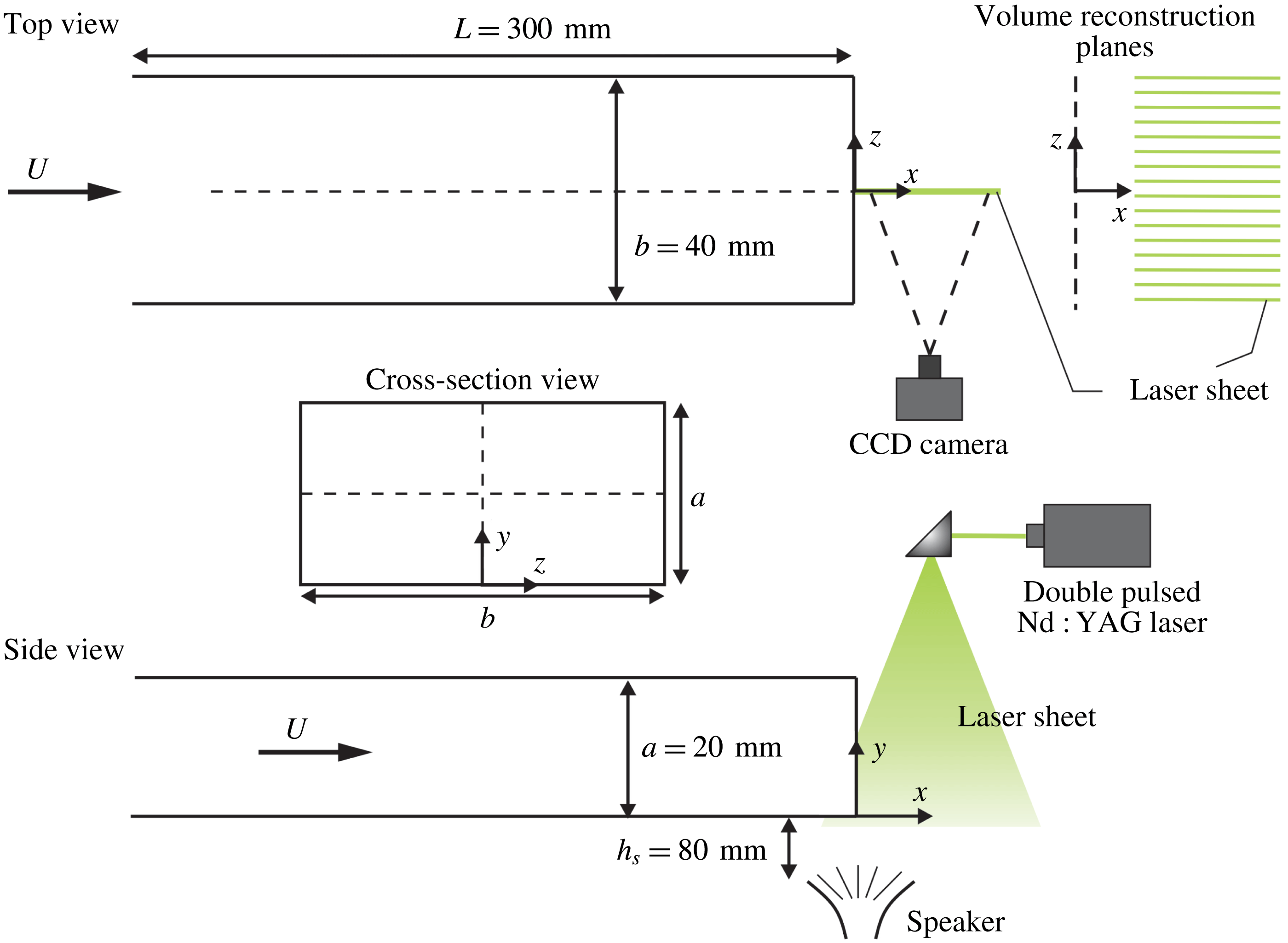
Experimental set-up: the schematic of the flow channel geometry and dimensions; the measurement components; planes of measurement.

2 Experiments
A schematic of the experimental set-up including the regions of interest, the flow channel geometry as well as the measurement components is presented in figure 1. Experiments are conducted at the outlet of a rectangular
 $20\times 40~\text{mm}^{2}$
duct with length
 $L=300~\text{mm}$
. The flow is supplied by a blower and passes through a flow conditioning unit consisting of a honeycomb insert and a set of three wire screens, followed by a 9 : 1 contraction. The flow enters the duct at turbulence intensities below 0.9 % and has mean flow uniformity within 0.25 % in the inviscid core. The flow rate is varied at the centreline velocities of
 $U=1,2,5,10,12.5,16,17.5,19,20~\text{m}~\text{s}^{-1}$
corresponding to the Reynolds numbers of
 $Re_{\unicode[STIX]{x1D703}_{0}}=U\unicode[STIX]{x1D703}_{0}/\unicode[STIX]{x1D708}=85,135,276,470,616,713,780,860,945$
where
 $\unicode[STIX]{x1D708}$
and
 $\unicode[STIX]{x1D703}_{0}$
denote kinematic viscosity and momentum thickness, respectively. The spatial dimensions are scaled using the
 $\unicode[STIX]{x1D703}_{0}$
value which is evaluated 20 mm downstream of the separation edge. It should be noted that, the velocities presented above are selected out of the measurements conducted for the range
 $U=1{-}40~\text{m}~\text{s}^{-1}$
and found sufficient to represent the transitioning characteristics of the phenomena under study.
Point-wise measurements are conducted using a Dantec 55P11 straight, general purpose single hot-wire (HW) probe oriented normal to the flow direction and connected to a Dantec Streamline Constant Temperature Anemometry system. The HW sampling rate is set to 16 kHz. The HW measurements are conducted over a time span of 32.8 s, corresponding to a total of
 $524\,288$
samples. Spectral analysis of the streamwise velocity fluctuations measured by the hot-wire is performed, with a frequency resolution bandwidth of at least 0.03 Hz. Following the HW, planar particle image velocimetry (PIV) is employed. The origin of the coordinate system is located at the centre of the duct with the
 $x$
-axis oriented in the streamwise direction. The
 $y$
-axis normal to the duct wall characterizes the span of the shear layer. The major components of the system include a dual pulsed Nd : YAG laser with a maximum output of
 $70~\text{mJ}~\text{pulse}^{-1}$
, a
 $1600~\times 1200~\text{pixel}$
14-bit Imager Pro X 2M CCD camera and a programmable timing unit. Laser sheet is formed using a combination of the cylindrical and spherical lenses, with a thickness of approximately 1 mm at its waist. The flow is seeded using a glycol–water-based fog with a mean particle diameter of
 $3~\unicode[STIX]{x03BC}\text{m}$
. The camera is equipped with a 60 mm fixed focal length lens and a
 $532~\mp 10~\text{nm}$
bandpass filter. The camera is synchronized with the laser by means of a timing unit controlled through the LaVision DaVis 8 software. PIV images are acquired in the
 $x$
–
 $y$
planes located at several
 $z/\unicode[STIX]{x1D703}_{0}$
. The camera sensor is cropped to
 $800\times 1200~\text{pixels}$
and the imaged field of view (FOV) is set to
 $24\times 36~\text{mm}$
. The velocity fields are computed by using the cross-correlation of pairs of successive images. The captured images are processed in the LaVision DaVis 8 software using an advanced multi-pass method where the initial and the final correlation passes are
 $64~\times 64~\text{pixels}$
with 50 % overlap and
 $24\times 24~\text{pixels}$
with 75 % overlap, respectively. This technique results in a vector pitch of 0.18 mm (measurement in the shear layer region), and the effective magnification of
 $0.38$
in the camera provides a pixel scale factor of
 $33~\text{pixels}~\text{mm}^{-1}$
. For the PIV measurement of the boundary layer at the separation edge, a vector pitch of 0.045 mm is achieved. The results are post-processed using the universal outlier detection (Westerweel & Scarano Reference Westerweel and Scarano2005) technique and the spurious vector removal with vector replacement. To produce time-averaged vector fields for each case,
 $3000$
image pairs are acquired at a rate of 14.73 Hz. The convergence of the results for the mean velocity, the root-mean-square (r.m.s.) of the streamwise velocity fluctuations and the
 $\langle Q\rangle$
criterion are checked using 1000, 1500, 2000, 2500 and 3000 instantaneous fields, and the 3000 snapshots are found to be more than sufficient for the time-averaged results. The random errors in the PIV measurements are evaluated using the particle image disparity method (Sciacchitano et al.
Reference Sciacchitano, Neal, Smith, Warner, Vlachos, Wieneke and Scarano2015), with the associated average in the velocity fields estimated to be less than 2 % within 95 % confidence for the free-stream region.
Characterization of the low (LA), mid (MA) and high (HA) amplitudes for the acoustic actuations at the fundamental and subharmonic frequencies.

Volume reconstruction of the flow fields is accomplished by performing the phase-locked PIV (Amitay, Tuna & DellOrso Reference Amitay, Tuna and DellOrso2016) measurements at multiple planes between
 $-10\leqslant z/\unicode[STIX]{x1D703}_{0}\leqslant 10$
spaced by
 $z/\unicode[STIX]{x1D703}_{0}=1.25$
. Acoustic excitation is provided by a sub-woofer placed at the outlet of the test section and the excitation signal served as the phase-locking reference signal for the PIV timing unit. Characterization of the low (LA), mid (MA) and high (HA) amplitudes for the acoustic actuations at the fundamental and subharmonic frequencies are presented in table 1. The natural/unperturbed case is characterized by a sound pressure level (SPL) of 91.2 dB at the centre of the channel exit. The effect of the acoustic excitation is characterized as 79.1 dB (LA), 88.1 dB (MA) and 95.5 dB (HA) at the same location when the tunnel is off. Based on these, each case can be defined as in table 1 by adding the free-stream noise level to the acoustic excitation noise level.
3 Results and discussion
3.1 Problem definition
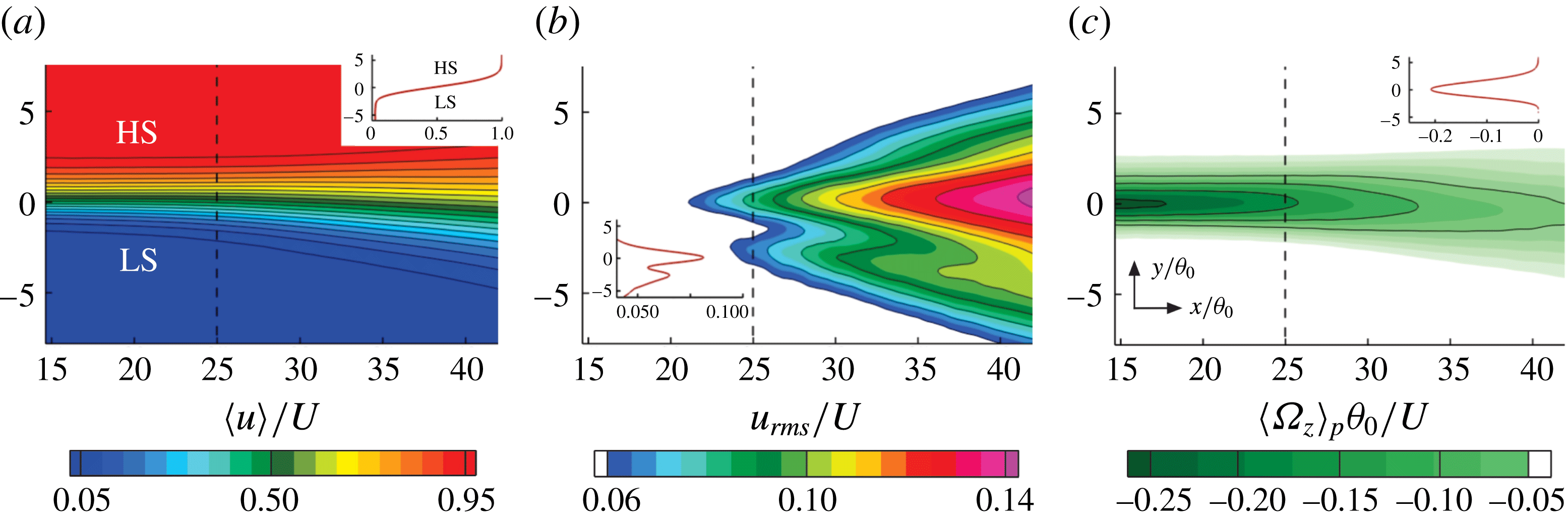
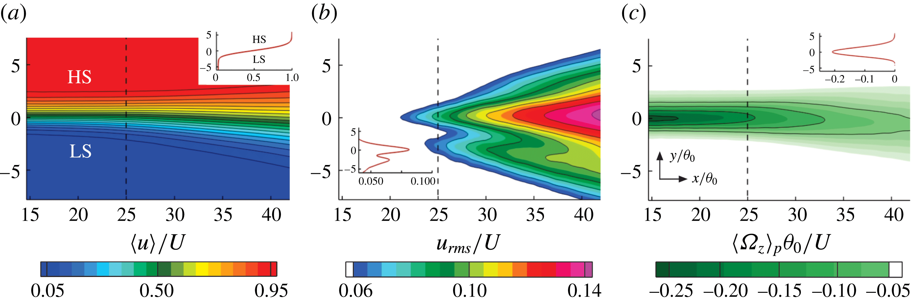
The general features of the present problem are introduced in figure 2 by illustrating the time-averaged streamwise velocity (
 $\langle u\rangle /U$
), the r.m.s. of the streamwise velocity fluctuations (
 $u_{rms}/U$
), as well as the vorticity component (
 $\unicode[STIX]{x1D6FA}_{Z}$
) normal to the plane of measurement for
 $Re_{\unicode[STIX]{x1D703}_{0}}=470$
. In figure 2(a), the time-averaged streamwise velocity contour is presented with the horizontal and the vertical axes characterizing the streamwise (
 $x/\unicode[STIX]{x1D703}_{0}$
) and the spanwise directions (
 $y/\unicode[STIX]{x1D703}_{0}$
), respectively. The spanwise variation of the velocity at the location of the vertical dashed line (
 $x/\unicode[STIX]{x1D703}_{0}=25$
) is shown with the profile at the upper-right corner. The high-speed (HS) and low-speed (LS) sides of the shear layer downstream of the separation edge are identified in the contour plot. They are also detectable on either side of the inflection point in the velocity line plot. The existence of an inflection point implies that the present flow field is prone to instabilities. In figure 2(b), the
 $u_{rms}/U$
contour is displayed with the corresponding line plot. It can be seen that two distinguishable peaks are detectable for the
 $u_{rms}$
. Hereafter, the peaks located towards the LS and the HS sides are referred to as the minor and the major peaks, respectively. We emphasize that, the LS and HS terms characterize the sides towards which the structures are oriented and not necessarily their exact location. As will be elaborated in the following sections, the individual peaks in the
 $u_{rms}$
react independently to the various active/passive flow control strategies. On the other hand, the shape of the vorticity profiles as shown in figure 2(c) remain unresponsive. Knowing the fact that the shearing and rotating fluid elements are not distinguishable by the vorticity field, the following sections of the study are motivated by the analysis of the shear/rotation interactions in the vicinity of the double peaking.
(a) Time-averaged streamwise velocity (
 $\langle u\rangle /U$
); (b) r.m.s. of the streamwise velocity fluctuations (
 $u_{rms}$
); (c) time-averaged vorticity (
 $\unicode[STIX]{x1D6FA}_{Z}$
). Profiles are extracted at the location of the vertical dashed line (
 $x/\unicode[STIX]{x1D703}_{0}=25$
). The low-speed and the high-speed sides of the shear layer are denoted as LS and HS, respectively.
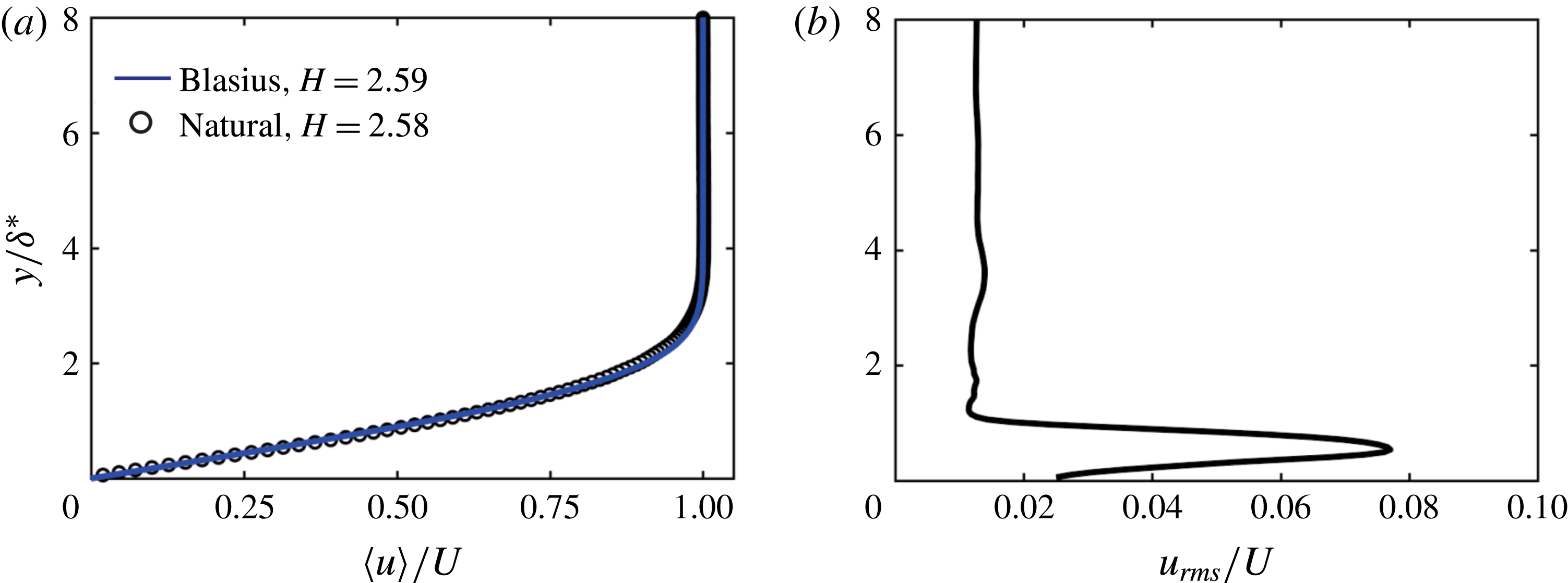
Boundary layer characteristics at the separation edge for
 $Re_{\unicode[STIX]{x1D703}_{0}}=470$
: (a) time-averaged streamwise velocity (
 $\langle u\rangle /U$
); (b) r.m.s. of the streamwise velocity fluctuations (
 $u_{rms}$
). The wall-normal distance (
 $y$
) is normalized by the local displacement thickness
 $\unicode[STIX]{x1D6FF}^{\ast }$
.

3.2 Incoming boundary layer at the separation edge
Before starting the main discussion of the results, a brief note on the incoming boundary layer characteristics at the separation edge would be beneficial. This is particularly important, since the double-peaked
 $u_{rms}$
profiles may also be observed in wall-bounded flows (Marusic & Kunkel Reference Marusic and Kunkel2003; Vassilicos et al.
Reference Vassilicos, Laval, Foucaut and Stanislas2015). Therefore, one would suggest this observation as the root for the occurrence of the double-peaked
 $u_{rms}$
in the separated shear layer formed in the downstream. Accordingly, the characteristics of the incoming boundary layer are presented in figure 3 for the
 $Re_{\unicode[STIX]{x1D703}_{0}}=470$
case which displays the double-peaking phenomenon for the naturally developing shear layer. The boundary layer velocity profile obtained from the PIV measurement is included in figure 3(a). The wall-normal distance (
 $y$
) is normalized by the local displacement thickness
 $\unicode[STIX]{x1D6FF}^{\ast }$
. The measured velocity profile has a shape factor of
 $H=2.58$
and resembles the Blasius boundary layer with
 $H=2.59$
. This characterizes a laminar incoming boundary layer at the separation edge. In addition, the streamwise turbulence intensity profile
 $u_{rms}$
shown in figure 3(b) depicts a single peak, and tends to diminish towards the free stream and near the wall region. This information rules out the possibility of the role of the boundary layer on the double-peaking phenomenon in the downstream shear layer.
3.3 Transitioning character of the double peaking and the shear/rotation
To investigate the correlation between the double peaking in the
 $u_{rms}$
and the competing effects of the shearing and the rotating regions of the flow, the
 $\langle Q\rangle$
criterion (Hunt, Wray & Moin Reference Hunt, Wray and Moin1988) is calculated from the time-averaged flow field. The advantage of the
 $\langle Q\rangle$
criterion over the vorticity is its capability of distinguishing between the purely shearing and rotating fluid elements. It should be noted that an instantaneous vortex dynamics analysis is carried out using the information obtained from the phase-locked PIV measurements and proper orthogonal decomposition (POD) in the following sections of the article. The
 $\langle Q\rangle$
criterion identifies the core of a vortex where the second invariant
 $(\langle Q\rangle )$
of the velocity gradient tensor is positive (Jeong & Hussain Reference Jeong and Hussain1995). Therefore, the
 $\langle Q\rangle$
criterion exhibits the local balance between the shear strain rate and the vorticity magnitude (Jeong & Hussain Reference Jeong and Hussain1995). Before investigating the hypothesis for the role of the shear/rotation dynamics in the double-peaking phenomenon, it would be beneficial to determine the flow regimes within which the peaks occur. To this end, a range of Reynolds numbers can be inspected through which the shear/rotation competition correlates with the double peaking in the
 $u_{rms}$
.
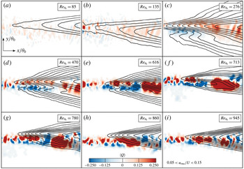
Selected from our measurements for a wide range of Reynolds numbers, the contours of the
 $\langle Q\rangle$
criterion superimposed on the iso-lines of
 $0.05\leqslant u_{rms}\leqslant 0.15$
for
 $Re_{\unicode[STIX]{x1D703}_{0}}=85,135,276,470,616,713,780,860,945$
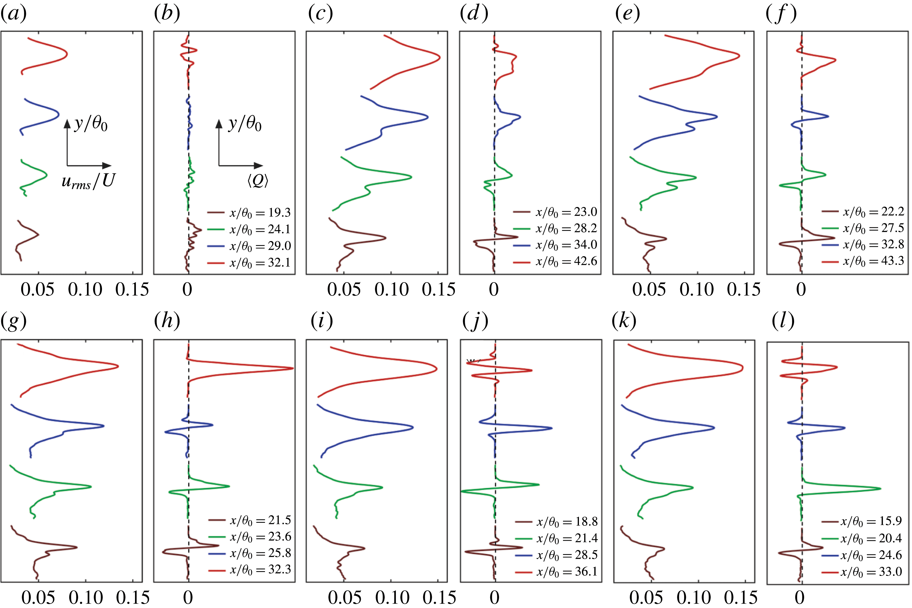
are illustrated in figure 4. It should be noted that the panels in figure 4 are restrained to the downstream locations where the initial KH roll-ups are more likely to take place. Negative (blue) clusters of the
 $\langle Q\rangle$
are associated with the shearing regions. On the other hand, the positive (red) spots represent the regions where the rotation of the fluid elements dominate. For the
 $Re_{\unicode[STIX]{x1D703}_{0}}=85$
and
 $135$
cases, the iso-lines show a single major peak with a tendency towards the high-speed side. For these two cases of the low Reynolds number, small-scale intermingled patches of the shear/rotation spots present a sporadic distribution. A second minor peak appears and develops near the low-speed side for
 $Re_{\unicode[STIX]{x1D703}_{0}}=276,470,616,713,780$
. This minor peak in the
 $u_{rms}$
profile seems to form at a certain streamwise location downstream of the separation edge. Subsequently, the minor peak tends to diminish and eventually disappears at farther downstream distances. Furthermore, the minor peak disappears for the Reynolds numbers larger than
 $Re_{\unicode[STIX]{x1D703}_{0}}=860$
. Another interesting observation is regarding the shear/rotation distribution obtained from the time-averaged flow fields at the presence of the minor peak. Either within the downstream locations or the Reynolds number ranges within which the double-peaked
 $u_{rms}$
occurs, the shear/rotation zones are not composed of the intermingled small spots. Instead, they portray two distinguished and well-organized layers (ribbons) of shear and rotation. Towards the low-speed side (not exactly on the LS side), a blue layer of shearing flow is observed at the vicinity of the minor peak of the
 $u_{rms}$
. On the contrary, the red ribbon of rotating zone appears at the proximity of the major peak of the
 $u_{rms}$
leaning towards the high-speed flow. It should be noted that, when we refer to the low-speed (LS) and the high-speed (HS) sides, the intention is not to specify the exact location of the structures. It is rather to indicate the side towards which a certain phenomenon is leaning to occur.
Time-averaged
 $\langle Q\rangle$
criterion superimposed by the iso-lines of the streamwise turbulence intensity
 $(0.05\leqslant u_{rms}/U\leqslant 0.15)$
for the naturally developing shear layer at
 $Re_{\unicode[STIX]{x1D703}_{0}}=85{-}945$
.

Streamwise turbulence intensity
 $(u_{rms}/U)$
correlated with the
 $\langle Q\rangle$
criterion at different streamwise locations
 $(x/\unicode[STIX]{x1D703}_{0}=19.3,24.1,29,32.1)$
in the naturally developing shear layer for
 $Re_{\unicode[STIX]{x1D703}_{0}}=85,276,470,780,860,945$
.

Time-averaged
 $\langle Q\rangle$
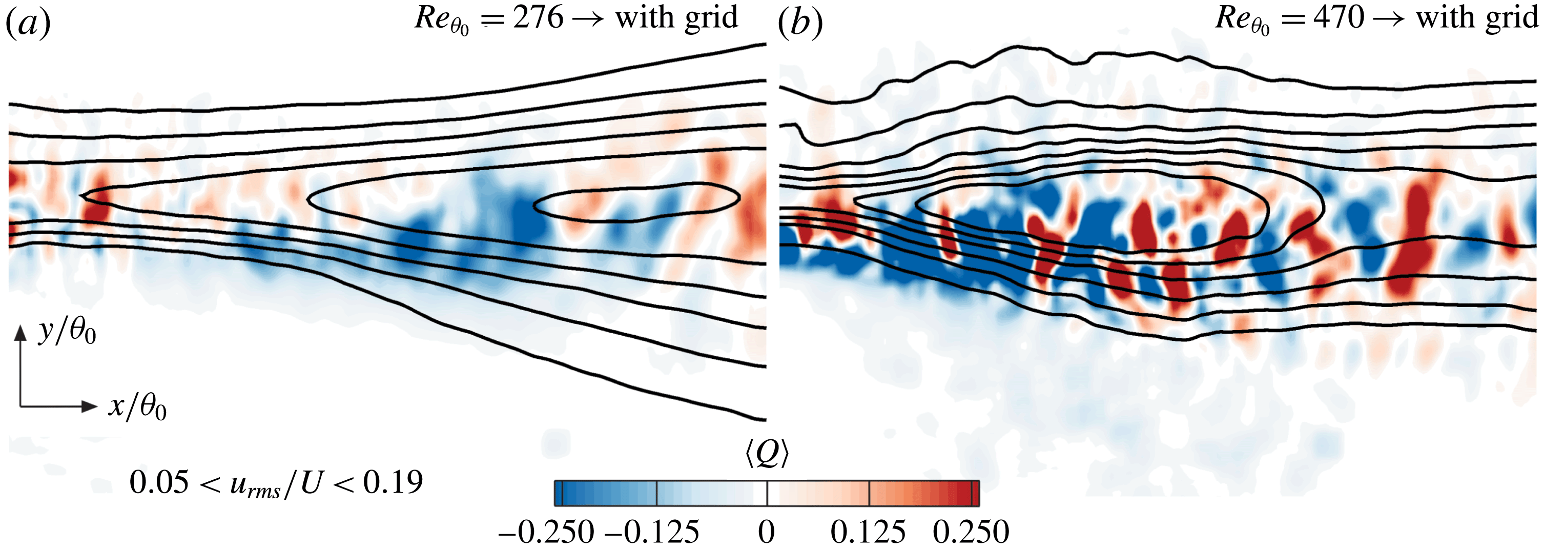
criterion superimposed on the iso-lines of the streamwise turbulence intensity
 $(0.05\leqslant u_{rms}/U\leqslant 0.19)$
for the naturally developing shear layers at: (a)
 $Re_{\unicode[STIX]{x1D703}_{0}}=276$
; (b)
 $Re_{\unicode[STIX]{x1D703}_{0}}=470$
cases subjected to the upstream grid turbulence.

In accordance with the formation and disappearance of the minor peak, the shear rotation distribution can also be associated with the transitional characteristics of shear layers. To further correlate the formation and decay of the minor peak with the shear/rotation distribution, figure 5 presents the spanwise variation of
 $u_{rms}$
correlated with the
 $\langle Q\rangle$
criterion for different streamwise locations (
 $x/\unicode[STIX]{x1D703}_{0}$
) for
 $Re_{\unicode[STIX]{x1D703}_{0}}=85,276,470,780,860,945$
. For the lowest Reynolds number (
 $Re_{\unicode[STIX]{x1D703}_{0}}=85$
), a single major peak is observed in the
 $u_{rms}$
profile at all streamwise locations. This is accompanied with the random small-scale variations of the shear (negative)/rotation (positive) quantities in the corresponding
 $\langle Q\rangle$
profiles. For the larger Reynolds numbers of
 $Re_{\unicode[STIX]{x1D703}_{0}}=276,470,780$
, a negative peak (shear) forms in the
 $\langle Q\rangle$
profiles and decays with the downstream distance. This co-occurs with the growth and the disappearance of the minor peak in the
 $u_{rms}$
profiles. For the higher ends of the transitioning locations or at the larger Reynolds numbers, the minor peaks in the
 $u_{rms}$
disappear and the organized correlation with the shear-characterizing peak in the
 $\langle Q\rangle$
is lost. As an example, the correlation is lost beyond the
 $x/\unicode[STIX]{x1D703}_{0}=21.4$
location for the
 $Re_{\unicode[STIX]{x1D703}_{0}}=860$
. Also, the profiles of the
 $Re_{\unicode[STIX]{x1D703}_{0}}=945$
are uncorrelated for all the streamwise locations.
Another important factor in forming the structure of the shear layers in the near-separation region is the level of the upstream turbulence and consequently the shape of the incoming boundary layer (Slessor, Bond & Dimotakis Reference Slessor, Bond and Dimotakis1998). To this end, the grid turbulence is introduced at the inlet of the channel for the above cases of the
 $Re_{\unicode[STIX]{x1D703}_{0}}=276$
and
 $470$
. As a result, the incoming boundary layer transitioned from laminar (
 $H=2.59$
) to turbulent (
 $H=1.5$
). The contours of the
 $\langle Q\rangle$
criterion superimposed on the iso-lines of
 $0.05\leqslant u_{rms}\leqslant 0.19$
are presented in figure 6. As a consequence of the grid turbulence, the above cases of the
 $Re_{\unicode[STIX]{x1D703}_{0}}=276$
and
 $470$
with the previous demonstration of the double peaking (in figure 4
c,d), now transition to the single-peaked
 $u_{rms}$
profiles. Likewise, the layered shear/rotation regions are dispersed and replaced by the more disorganized intermingling spots. Up to this point, three important observations suggest the transitioning character of the double-peaking phenomenon and the corresponding shear/rotation distributions. This transitioning behaviour is commonly attributed to the nature of the shear layer formation and the associated phenomena. First, the double peaking in the
 $u_{rms}$
profile occurs and correlates with the shear/rotation distribution within a certain range of the Reynolds numbers below and above which the correlation/occurrence is lost. Second, the formation, evolution and the decay of the double peaking and the corresponding organization of the shear/rotation starts at a certain downstream location, maintains its character up to a distance farther downstream after which it disappears. Third, development of the separated boundary layer into the transitioning/turbulent states as well as the elevated upstream turbulence levels due to the grids, alter the transition of the double peaking and the organization of the shear/rotation spots.
3.4 Frequency considerations
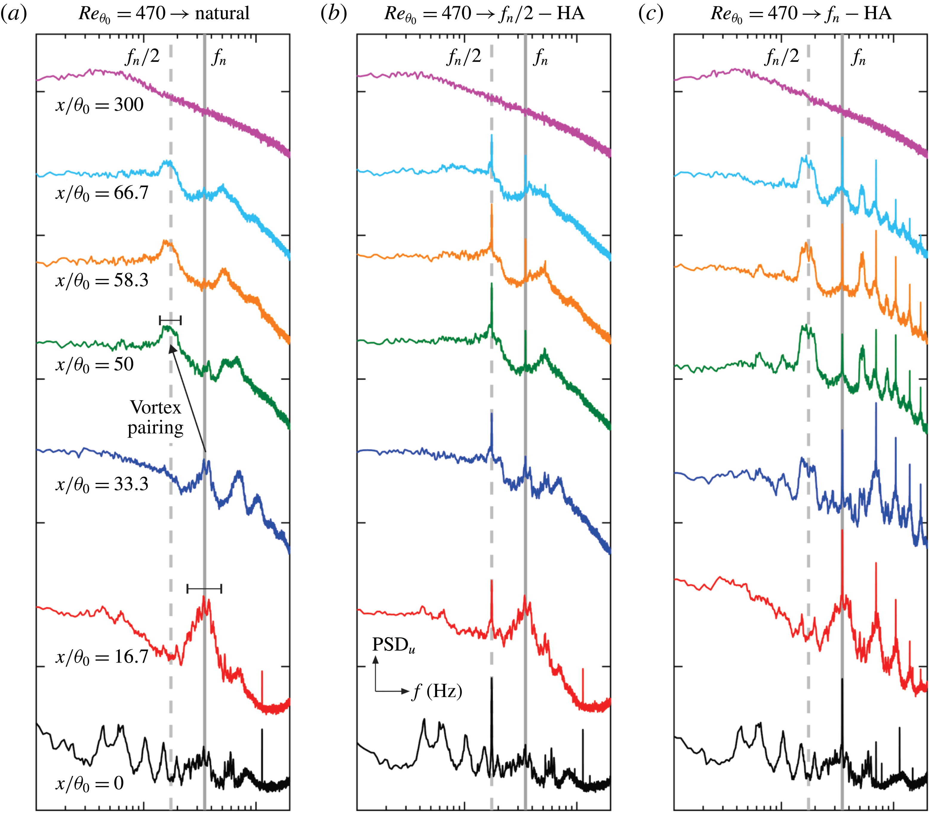
The literature survey presented in the introduction section suggests the phenomenon under investigation is associated with the interaction of the fundamental and the subharmonic modes. Therefore, the corresponding frequencies should be first determined for the naturally developing shear layer. Afterwards, the frequencies characterizing the fundamental and the subharmonic modes can be used to acoustically actuate the flow at different amplitudes. To this end, HW measurements are utilized to obtain the streamwise velocity spectrum at different downstream locations (
 $x/\unicode[STIX]{x1D703}_{0}=0{-}300$
) for the
 $Re_{\unicode[STIX]{x1D703}_{0}}=470$
which portrayed the double-peaking behaviour. Figure 7 presents the frequency spectra of the streamwise velocity fluctuations obtained from the HW measurements at different axial locations. The vertical dashed and solid lines characterize the frequencies associated with the subharmonic (
 $f_{n}/2=175~\text{Hz}$
) and the fundamental (
 $f_{n}=350~\text{Hz}$
) modes, respectively. At the
 $x/\unicode[STIX]{x1D703}_{0}=0$
location seen in figure 7(a), the natural case maintains the upstream boundary layer characteristics without any frequency preference. It should be noted that the high-frequency spike at this location is associated with the apparatus noise which is significantly larger than the natural frequency of interest. On the other hand, forcing the shear layer at the subharmonic (figure 7
b) and the fundamental (figure 7
c) modes create the sharp spikes in the velocity spectrum at
 $x/\unicode[STIX]{x1D703}_{0}=0$
for the corresponding frequency. At
 $x/\unicode[STIX]{x1D703}_{0}=16.7$
, the naturally developing shear layer forms a broadband peak, which is commonly seen in shear layers (Ho & Huerre Reference Ho and Huerre1984; Hussain & Zaman Reference Hussain and Zaman1985). The highest peak almost located in the middle of the broadband characterizes the dominance of the fundamental mode and accordingly the roll-up frequency. The equivalent dimensionless frequency, is determined based on the Strouhal number (
 $St_{\unicode[STIX]{x1D703}_{0}}=f_{n}\unicode[STIX]{x1D703}_{0}/U=0.026$
) which is close to the reported value of
 $0.024$
(Hussain & Zaman Reference Hussain and Zaman1985). Farther downstream at
 $x/\unicode[STIX]{x1D703}_{0}=33.3$
, the higher harmonic peaks start to appear. This is the consequence of the nonlinear perturbations setting in (Hussain & Zaman Reference Hussain and Zaman1985). Beyond this streamwise location, the energy content of the fundamental mode starts to diminish until it vanishes within the range of
 $x/\unicode[STIX]{x1D703}_{0}=50{-}66.7$
streamwise locations. This is also accompanied by the formation and growth of the subharmonic peak. This phenomenon, appearing as the shifting of the peak towards the lower frequencies with the downstream distance, follows the previous observations by Hussain & Zaman (Reference Hussain and Zaman1985). The frequency associated with the subharmonic demonstrates a value of half of the fundamental mode. This occurs because the passage frequency of the vortices is halved due to the vortex pairing in the downstream of the roll-up location. For the case of the subharmonic actuation, a sharp spike is observed for the
 $f_{n}/2$
frequency. Accordingly, the corresponding mode tends to dominate the fundamental mode earlier. On the other hand, actuating the fundamental mode advances the formation of the nonlinear effects and the appearance of the higher harmonic spikes. In the far-field region at
 $x/\unicode[STIX]{x1D703}_{0}=300$
, none of the cases show a frequency preference and hence the isotropic fully developed turbulence introduces wide ranges of frequencies. In this region, the contribution of the high-frequency (short wavelength) small-scale eddies is increased and the mixing is consequently enhanced.
Spectra of the streamwise velocity fluctuations at different streamwise locations (
 $x/\unicode[STIX]{x1D703}_{0}=0{-}300$
) obtained from the HW measurements at
 $Re_{\unicode[STIX]{x1D703}_{0}}=470$
for: (a) natural case; (b) actuation of the subharmonic mode (
 $f_{n}/2$
) at the high amplitude (HA); (c) actuation of the fundamental mode (
 $f_{n}$
) at the high amplitude (HA).

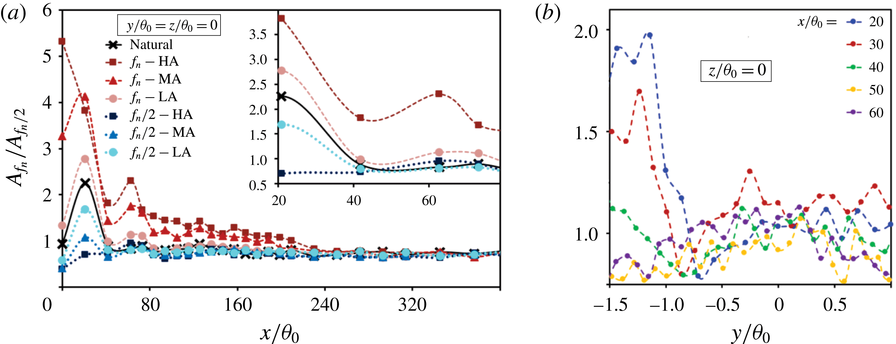
Fundamental (
 $f_{n}$
) to subharmonic (
 $f_{n}/2$
) amplitude ratio of the velocity spectra obtained from the HW measurements for
 $Re_{\unicode[STIX]{x1D703}_{0}}=470$
: (a) streamwise variation at (
 $y/\unicode[STIX]{x1D703}_{0}=z/\unicode[STIX]{x1D703}_{0}=0$
) for the fundamental and subharmonic forcing of the shear layers at the low (LA), mid (MA) and the high (HA) amplitudes; (b) spanwise variation at (
 $x/\unicode[STIX]{x1D703}_{0}=20,30,40,50,60$
) streamwise locations and (
 $z/\unicode[STIX]{x1D703}_{0}=0$
) for the natural case.

Spatial theory of the linear stability (LST) analysis based on the PIV measurements for the natural, fundamental
 $(f_{n})$
and subharmonic
 $(f_{n}/2)$
actuations at low (LA), mid (MA) and high (HA) amplitudes: (a–f) growth rate
 $(-\unicode[STIX]{x1D6FC}_{i})$
variation of the range of frequencies with the downstream distance; (g,h) the cumulative integral of the growth rate (
 $N$
-factor) associated with the fundamental and the subharmonic modes; (
 $i$
) fundamental to subharmonic growth rate ratios
 $(-\unicode[STIX]{x1D6FC}_{i}(f_{n})/-\unicode[STIX]{x1D6FC}_{i}(f_{n}/2))$
.

In figure 8, the amplitude ratios corresponding to the fundamental and the subharmonic modes are extracted from the velocity spectra and presented as
 $(A(f_{n})/A(f_{n}/2))$
for the
 $Re_{\unicode[STIX]{x1D703}_{0}}=470$
. The streamwise variation of the amplitude ratio shown in figure 8(a) confirms the dominant effect of the fundamental mode near the separation region for the natural case. With the downstream distance, the amplitude ratio is decreased as the fundamental mode declines and the subharmonic effects dominate due to vortex pairing. Excitation at low (LA), mid (MA) and high (HA) amplitudes amplifies the energy content of the corresponding
 $f_{n}$
or
 $f_{n}/2$
frequency. Beyond
 $x/\unicode[STIX]{x1D703}_{0}=240$
, none of the modes dominate as the shear layer demonstrates fully developed characteristics where the high-frequency small scales become important. This observation limits the focus of our study to the near-field region where the competing effects of the fundamental and the subharmonic modes are strong. The traverse distribution of the amplitude ratio is presented in figure 8(b) at the streamwise locations
 $x/\unicode[STIX]{x1D703}_{0}=20,30,40,50,60$
in the
 $z/\unicode[STIX]{x1D703}_{0}=0$
plane for the naturally developing shear layer. At
 $x/\unicode[STIX]{x1D703}_{0}=20{-}30$
, the fundamental mode prevails with a stronger domination on the low-speed side. This is a verification of the KH roll-ups occurring towards the low-speed outside region as also reported in the velocity spectra by Hussain & Zaman (Reference Hussain and Zaman1985). Up to
 $x/\unicode[STIX]{x1D703}_{0}=40$
, which is located within the vortex pairing region, the fundamental mode loses its energy content until the subharmonic dominates beyond
 $x/\unicode[STIX]{x1D703}_{0}=50$
.
The fundamental and the subharmonic frequencies detected above, for the naturally developing shear layers and their behaviour under the actuation, are obtained owing to the temporally high-resolution HW velocity measurements. To verify this analysis, spatial linear stability (LST) analysis is conducted based on the spatially resolved PIV measurements. In the hydrodynamic theory of stability, the shear layer is then treated as the counteraction among the ensemble of propagating instability waves (Michalke Reference Michalke1972; Drazin & Reid Reference Drazin and Reid2004; Betchov Reference Betchov2012). Each of the waves, the amplitude of which may grow/decay in time/space as they advect downstream, are associated with the flow structure of a certain length scale (wavelength). This concept is achieved by the analysis of the flow in a Fourier space rather than in a physical time/space domain. In the spatial analysis, the perturbations are only allowed to grow/decay in space. The disturbances may only be convected in time without amplification/damping. To this end, the least squares method is implemented for the curve fitting of the local velocity profiles obtained from the PIV measurements according to Dini, Seligt & Maughmert (Reference Dini, Seligt and Maughmert1992). The hyperbolic–tangent velocity profile is typically used to conduct the spatial linear stability analysis, namely in the study of the effect of the shear layer velocity ratio on the growth of the perturbations in space (Monkewitz & Huerre Reference Monkewitz and Huerre1982). The Orr–Sommerfeld equation can be derived by introducing perturbations to the linearized incompressible Navier–Stokes equations assuming the normal mode disturbances (Schmid & Henningson Reference Schmid and Henningson2012). It should be noted that for individual natural or actuated cases, different base flows are considered. More specifically, the time-averaged velocity field measured by the PIV is extracted at certain locations and used for the LST. It should also be noted that, the spatial LST has previously been used for actuated flows, namely by Marxen et al. (Reference Marxen, Kotapati, Mittal and Zaki2015) and Yarusevych & Kotsonis (Reference Yarusevych and Kotsonis2017). For each downstream location, implementation of the time-averaged streamwise velocity profile as the base flow, signifies a local LST analysis of the spatial perturbations. After implementing the proper homogeneous boundary conditions, the resulting eigenvalue problem needs to be solved. The Orr–Sommerfeld equation is then solved by the spectral colocation approach, where the Chebyshev polynomials provide the approximation of the eigenfunctions. The nonlinearity issue in the eigenvalue system is resolved by means of the companion matrix according to Bridges & Morris (Reference Bridges and Morris1984). Compared to the other traditional methods such as the finite difference schemes, implementing the spectral method based on the Chebyshev polynomials provides enhanced accuracy (Orszag Reference Orszag1971). The higher-order spectral methods converge faster and are computationally more affordable as they demand less processing power and physical memory.
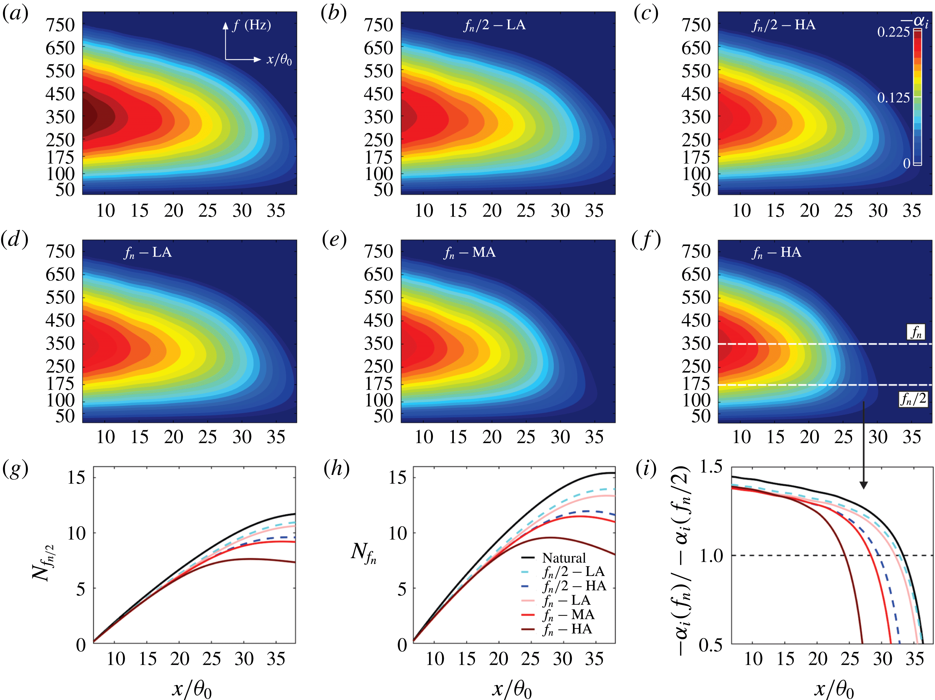
LST results are presented in figure 9 for the natural and the forced cases at the fundamental
 $(f_{n})$
and the subharmonic
 $(f_{n}/2)$
frequencies for the low (LA), medium (MA) and high (HA) excitation amplitudes. The contour plots in figure 9(a–f) display the downstream variation of the growth rates
 $(-\unicode[STIX]{x1D6FC}_{i})$
associated with a range of frequencies obtained from the LST for
 $Re_{\unicode[STIX]{x1D703}_{0}}=470$
. In the near-separation region of the natural case, a range of frequencies contribute to the growth of the instabilities. However, the fastest growing wave is associated with the 350 Hz frequency characterizing the fundamental (
 $f_{n}$
) mode at which the roll-up occurs. This verifies the broadband peak previously discussed for the velocity spectra. Another interesting observation is that the LST contours illustrate meaningful results almost up to
 $x/\unicode[STIX]{x1D703}_{0}=30$
beyond which the velocity spectra detected the emergence of the nonlinear effects. This is more evident by the shrunk contour region in the
 $f_{n}-\text{HA}$
actuation case for which the LST validity deteriorates earlier. This is a meaningful observation when restating that the high amplitude actuation at the fundamental frequency depicts advanced location of the nonlinear peaks in the velocity spectra.
A common way of presenting the downstream variation of the growth rate is by calculating its cumulative integral over the streamwise distance known as the
 $N$
-factor. This parameter is also called the amplification factor and is a measure of the flow transition (Smith & Gamberoni Reference Smith and Gamberoni1956; Van Ingen Reference Van Ingen1956, Reference Van Ingen2008). Figure 9(g,h) depicts the
 $N$
-factor profiles corresponding to the fundamental and the subharmonic modes obtained for the naturally developing and the actuated shear layers. The profiles characterize an initial linear increase with the downstream distance. After reaching its critical value at the maxima, the
 $N$
-factor profile start a decreasing trend. This reduction after the critical value demonstrates the saturation of the instabilities and characterizes the start of the transition (Yarusevych & Kotsonis Reference Yarusevych and Kotsonis2017). The occurrence of the transition precedes for the forced cases as they earlier reach a nonlinear state.
In addition, the
 $N$
-factor is related to the amplitude of the disturbances (
 $a$
) through the equation
 $a/a_{0}=\text{e}^{N}$
, where
 $a_{0}$
is the reference value. Accordingly, the critical value of the
 $N$
-factor is equivalent to the saturation limit of the perturbations beyond which the transition occurs. By visual inspection of the slope in the linear region of the
 $N$
-factor, the rates at which the perturbations grow with the downstream distance can be analysed. Comparing the naturally developing shear layers within this linear region, it becomes evident that the fundamental mode grows at a higher rate with respect to the subharmonic frequency. The actuated shear layers tend to saturate earlier and hence the transition is advanced. Particularly, actuation at the fundamental frequency reaches the transition earlier due to the advanced roll-up. Similarly, increasing the amplitude of the excitations advances the transition as the earlier domination of the nonlinear effects reach up to the transition state earlier. In figure 9(i), the fundamental to the subharmonic growth rate ratios
 $(-\unicode[STIX]{x1D6FC}_{i}(f_{n})/-\unicode[STIX]{x1D6FC}_{i}(f_{n}/2))$
are presented. Within the expected range of validity of the linear stability analysis, the fundamental mode dominates in the near-separation region. With the farther downstream distances, the subharmonic mode tends to grow faster. This is also in accordance with the previous observations in the HW-based velocity spectra. The fundamental to the subharmonic growth rate ratios tends to fall below unity at certain streamwise locations for each of the natural and the actuated cases. These locations coincide with the point of the saturation in the
 $N$
-factor profiles discussed above.
3.5 Acoustic control of the shear/rotation
The discussions up to this point reveal the transitioning character of the double-peaking phenomenon, with the Reynolds number, the downstream distance and the upstream grid-induced turbulence. It is also shown that the double-peaking in the r.m.s. of the streamwise velocity fluctuations is correlated with the shear/rotation distribution obtained from the time-averaged flow field. However, the time-averaged analysis conducted earlier, only provides the global aspects of the shear/rotation dynamics. For a better understanding of the local features, the shear/rotation is analysed in the context of the instantaneous vortex dynamics presented in this section. The intention is to control a case with the existence of the double peaking through the acoustic altering of the vortex dynamics. The instantaneous speculations are then generalized using the statistical analysis of the vortex core locations.
Proper orthogonal decomposition (POD) is implemented to reconstruct the flow field of the natural and the actuated cases at
 $Re_{\unicode[STIX]{x1D703}_{0}}=470$
using the five most energetic modes. This is achieved by recovering the 79–85 % of the total energy in the flow. The mean of the snapshots are subtracted prior to conducting the POD. Afterwards, the r.m.s. of the streamwise velocity fluctuations (
 $\tilde{u} _{rms}/U$
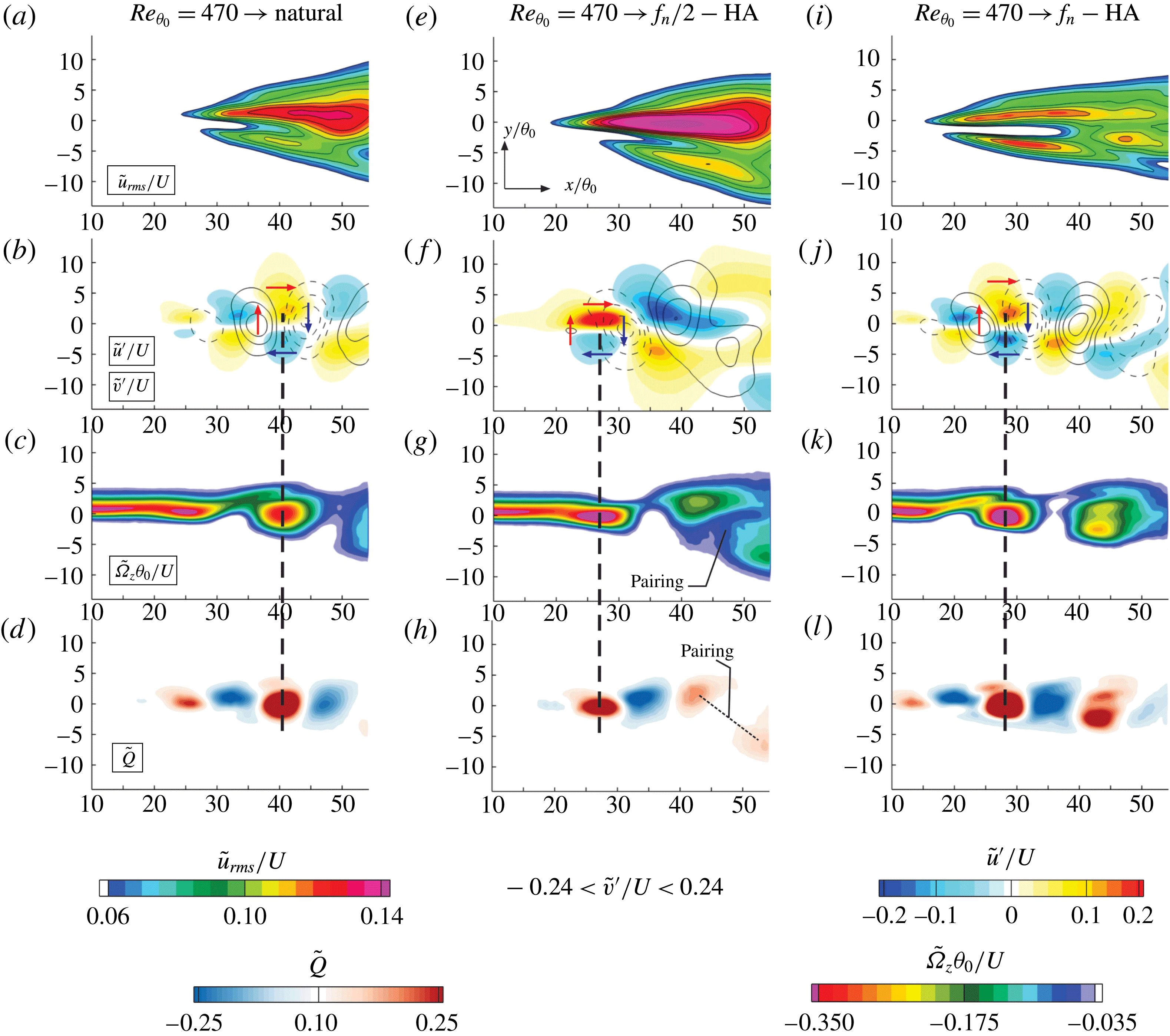
) is calculated using the POD field and displayed in figure 10(a,e,i) for the natural, subharmonic and the fundamental actuation cases, respectively. At first glance, the r.m.s. field obtained from the POD demonstrates a cleaner image with the peaks displayed more clearly compared to that of the originally presented data. POD reproduces the time-averaged PIV results with clearly defined double peaks by filtering out the small-scale high-frequency modes. It can be seen that the actuation of the shear layer at the fundamental mode amplifies the minor peak, which tends to form near the low-speed region. In addition, the formation location of the minor peak in the streamwise distance is advanced under the actuation of the fundamental mode. On the other hand, excitation at the subharmonic frequency amplifies both the major and the minor peaks. However, the major peak located towards the high-speed region is more significantly affected. The vortex pairing mechanism, and the associated subharmonic effect, are known to expand the shear layer (Freymuth Reference Freymuth1966; Winant & Browand Reference Winant and Browand1974) in the traverse direction. This is also evident in figure 10(e) where the
 $\tilde{u} _{rms}/U$
field corresponding to the subharmonic forcing, covers a broader traverse region compared to the natural and the fundamental actuation cases.
In figure 10(b,f,j), the instantaneous streamwise velocity fluctuations (
 $\tilde{u^{^{\prime }}}/U$
) coloured from blue (
 $-0.2$
) to red (0.2) are given for the natural, subharmonic and the fundamental actuation cases, respectively. The corresponding spanwise velocity fluctuations (
 $\tilde{v^{^{\prime }}}/U$
) are presented as dashed (
 $-0.24$
) and solid (0.24) lines. The local direction associated with each of the fluctuating regions is depicted by a horizontal or vertical arrow for the streamwise and spanwise directions, respectively. As stated earlier, the Kelvin–Helmholtz instability initiates the growth of the disturbances in the shear layer. That would be the case of having only two horizontal arrows, generating a differential of the streamwise velocity with respect to the traverse direction. This generates an elongated layer between the pair of horizontal arrows and a friction (shear) region is formed. Farther downstream, as the instabilities grow, another pair of the vertical arrows appear and create a differential of the spanwise velocity with respect to the streamwise direction. The resulting four-arrow configuration is illustrated in figure 10(b,f,j), where the two pairs of the streamwise and spanwise shear arrows create a spinning around a centre of rotation. This observation clearly characterizes a shear/rotation cell which we know as the vortex core. In other words, the coupling between the shear and rotation is the engine to the formation of a vortex through the roll-up process.
Proper orthogonal decomposition (POD): streamwise turbulence intensity
 $\tilde{u} _{rms}/U$
; streamwise (
 $\tilde{u^{^{\prime }}}/U$
, blue to red) and spanwise (
 $\tilde{v^{^{\prime }}}/U$
, dashed lines) fluctuations; vorticity
 $\tilde{\unicode[STIX]{x1D6FA}}_{Z}$
and
 $\tilde{Q}$
: (a–d) natural; (e–h) subharmonic forcing at the high amplitude (
 $f_{n}/2-\text{HA}$
); (i–l) fundamental forcing at the high amplitude (
 $f_{n}-\text{HA}$
); arrows show the direction of the local shear and the sense of rotation of the corresponding vortex core.

This observation translates into the instantaneous vorticity
 $\tilde{\unicode[STIX]{x1D6FA}}_{Z}$
dynamics in the corresponding POD reconstructions presented in figure 10(c,g,k). The case of the pair of horizontal arrows is basically the near-separation region where the elongated (stretched) vorticity layer is formed. Farther downstream, the accumulated vorticity field is associated with the angular velocity of the flow the direction of which is depicted by the four-arrow arrangement described above. Another observation is recognized as the phase-reversal phenomenon which is described by Sato (Reference Sato1956, Reference Sato1959, Reference Sato1960) and Browand (Reference Browand1966). They found that the amplitude of the fluctuations reduce to zero at a certain traverse location and then grows on the other side with the opposite phase. The four-arrow arrangement of the present study and its correlation with the shear/rotation zones explain this phenomenon by the straightforward visualization of the flow features. Each pair of parallel arrows with opposite directions simply portray the phase reversal of the fluctuations. Also, the fluctuations vanish at a traverse location between the two horizontal arrows. The traverse location is found near the centre of rotation, which is detected slightly towards the low-speed side. This finding is in accordance with Michalke (Reference Michalke1965), who stated that the traverse location does not fall on the critical layer and it is rather located towards the low-speed side.
The POD reconstruction of the
 $\tilde{Q}$
criterion clearly describes the rotating vortex core in figure 10(d,h,l). With the aid of the vertical dashed lines, the rotation of the vortex core is correlated with the centre of rotation of the four-arrow arrangement as well as the accumulated vorticity region. In addition, the instantaneous
 $\tilde{Q}$
criterion distinctively represents the shear and the rotation areas. The shear regions in the
 $\tilde{Q}$
criterion can be associated with the thinning in the stretched (elongated) vorticity layer. The streamwise location of the first KH roll-up is advanced under the actuation of the fundamental mode. Accordingly, the minor peak of the
 $\tilde{u} _{rms}$
is also augmented and appears at more upstream locations. It should be noted that the KH roll-ups occur towards the low-speed side where the minor peak of the
 $\tilde{u} _{rms}$
is also observed. Actuation of the subharmonic mode enhances the occurrence of the vortex pairing. As illustrated in figure 10(g,h) during the pairing, the upstream vortex core accelerates and shifts towards the high-speed side and catches up with the decelerated downstream rotation core. Concurrently, the downstream vortex core is pushed towards the low-speed region. As a result, both the major and the minor peaks are amplified. However, the major peak which leans towards the high-speed side is more strongly intensified. In addition, organization of the pair of the merging rotating cores in a wider traverse region is accompanied by a larger r.m.s. field of the streamwise velocity fluctuations.
Above observations in the instantaneous flow field, shed more light on the role of the vortex dynamics in the double peaking and its association with the roll-up and the pairing processes. However, it is important to determine whether the occurrence of these phenomena are statistically sufficient to affect the r.m.s. values. To this end, a vortex core detection algorithm is utilized based on the
 $\unicode[STIX]{x1D6E4}_{2}$
criterion introduced by Graftieaux, Michard & Grosjean (Reference Graftieaux, Michard and Grosjean2001). This method is found to identify the vortex core more precisely as the centre of rotation (Graftieaux et al.
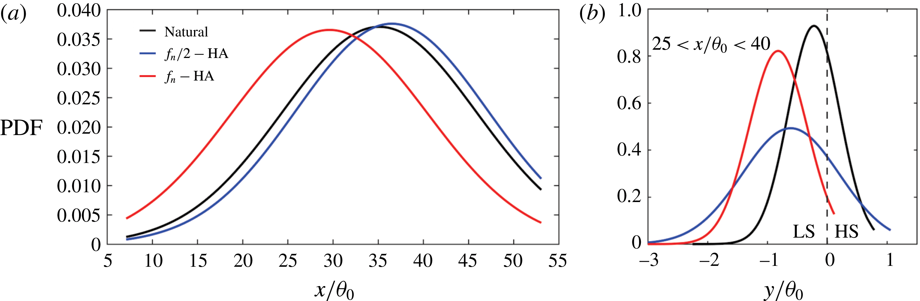
Reference Graftieaux, Michard and Grosjean2001). The total number of detected vortices in the measurement frames are counted over 3000 time instants and used for the statistical examination. The spatial statistics of the vortex locations are presented in terms of the probability density function (PDF) in figure 11 for the natural and the actuated shear layers. The PDF associated with the natural case demonstrates that the majority of the vortices are detected within the
 $x/\unicode[STIX]{x1D703}_{0}=30{-}40$
streamwise locations. The vortex count increases with the downstream distance due to the roll-up and then drops due to the pairing. The subharmonic actuation does not demonstrate a major difference compared with the naturally evolving shear layer. On the other hand, the PDF is evidently shifted upstream for the shear layer actuated at the fundamental frequency. This observation reveals the advanced location of the KH roll-ups for the shear layers forced under the fundamental frequency. In addition, the total number of vortices is found to increase by 21 % due to the actuation of the fundamental mode. Since the KH roll-ups tend to occur towards the low-speed side of the shear layer, the outcome is observed in the augmentation of the minor peak in the
 $u_{rms}$
. Moreover, the minor peak location is also advanced in accordance with the KH roll-ups.
Probability density function (PDF) of the spatial statistics of the vortex core locations for the natural and actuated cases: (a) streamwise distribution; (b) traverse distribution within the
 $x/\unicode[STIX]{x1D703}_{0}=30{-}40$
streamwise locations. The vortex core locations are detected using the
 $\unicode[STIX]{x1D6E4}_{2}$
criterion for the natural, fundamental
 $(f_{n})$
and subharmonic
 $(f_{n}/2)$
actuations at the high amplitude (HA).

The PDFs presented in figure 11(b) exhibit the traverse distribution of the vortex core locations within the range of the downstream locations in which the pairing is expected to happen according to the velocity spectra shown earlier. The PDFs associated with the actuation at the fundamental mode display a flatness similar to that of the natural case. However, the PDF peak is shifted towards the low-speed side in accordance with increased KH roll-ups when forcing the shear layer at the fundamental frequency. Also, this PDF is clustered around its mean traverse location. On the other hand, actuation at the subharmonic mode generates a wider PDF where the vortex locations are more deviated from the mean and are more uniformly distributed in the traverse direction. The wider PDF under the subharmonic actuation is a sign of the shear layer expansion which is known to occur due to the vortex pairing (Winant & Browand Reference Winant and Browand1974). Traverse statistics of the
 $f_{n}/2$
excitation case reveals occurrence of more vortex cores near both the high-speed and the low-speed sides compared to the fundamental mode actuation. This verifies our discussions in the instantaneous analysis of the vortex pairing. The upstream vortex is shifted towards the high-speed side during the merging and the major peak of the
 $u_{rms}$
is amplified. In contrast, the downstream vortex is shifted towards the low-speed side and the minor peak of the
 $u_{rms}$
is augmented. Even though both of the
 $u_{rms}$
peaks are affected, the peak on the high-speed side is more strongly intensified. It should also be noted that the total number of the vortices drops by 23 % when the shear layer is actuated at the subharmonic mode. This signifies the vortex pairing enhancement when forcing the flow under the subharmonic mode.
Volumetric topologies of the shear/rotation loops obtained from the phase-locked PIV measurements. Instantaneous phases (
 $\unicode[STIX]{x1D719}=0^{\circ },60^{\circ },120^{\circ },180^{\circ }$
,
 $240^{\circ },300^{\circ }$
) of the shear (blue) and rotation (red) loops of the
 $\langle Q\rangle _{p}$
criterion passed through the vorticity cut planes (green) at for the fundamental actuation at high amplitude (
 $f_{n}-\text{HA}$
). Supplementary movie is available at https://doi.org/10.1017/jfm.2018.214.

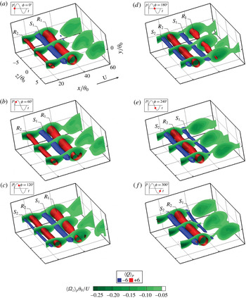
As discussed, the vorticity field provides a realistic visualization of the shear layer elongated regions, accumulated rotating vortex roll-ups as well as the pairing phenomenon (Zabusky & Deem Reference Zabusky and Deem1971; Saffman & Baker Reference Saffman and Baker1979; Aref & Siggia Reference Aref and Siggia1980). However, it would be more beneficial to distinguish between the shear/rotation regions and correlate them with the vorticity distribution. Spatio-temporal formation/advection of the distinguished shear(blue)/rotation(red) loops are animated in figure 12. After conducting the phase-locked PIV measurements in multiple planar fields of view, the three-dimensional topologies are obtained by interpolating the FOVs into the volumetric information. The resulting
 $\langle Q\rangle _{p}$
-criterion obtained for the high amplitude actuation of the fundamental mode, during the period of the acoustic excitation, are presented at the phases
 $\unicode[STIX]{x1D719}=0^{\circ },60^{\circ },120^{\circ },180^{\circ },240^{\circ },300^{\circ }$
. The rotation loops are formed near the separation edge, entrain the ambient fluid and grow in time/space due to the viscous diffusion while convecting downstream. The shear loops are identified with the shear layer thinning in the stretched vorticity zones while the rotating loops intersect with the expansion/accumulation in the vorticity cut planes. The first rotating loop (
 $R_{1}$
) is followed by the shear loop (
 $S_{1}$
) and the second vortex loop (
 $R_{2}$
) during the phases
 $\unicode[STIX]{x1D719}=0^{\circ }{-}60^{\circ }$
. During
 $\unicode[STIX]{x1D719}=120^{\circ }{-}180^{\circ }$
, the shear loop
 $S_{2}$
enters the domain while the previous loops are advected farther downstream and grown in radius. The rotation core
 $R_{1}$
exits the domain during
 $\unicode[STIX]{x1D719}=240^{\circ }{-}300^{\circ }$
and the expected phase
 $\unicode[STIX]{x1D719}=360^{\circ }$
to complete a cycle is equivalent to
 $\unicode[STIX]{x1D719}=0^{\circ }$
.
The radial expansion of the vortex cores with the downstream distance is due to the influence of the friction, through the viscous diffusion process in the vorticity field. Initially, when the vorticity is accumulated in the vortex core, it is subjected to high gradients. At the presence of such high vorticity gradients, the viscous diffusion effects are stronger. As a result, while conserving the total vorticity, its region of effectiveness is expanded. Accordingly, the strength of the vortex core is gradually diminished as the vorticity field becomes smooth (diffused). It should be noted that with the appearance of the small scales, the viscous diffusion occurs at smaller time scales and hence the dissipation dominates. Another important aspect of the viscous diffusion phenomenon is its indirect effect on the velocity at which the rotating vortex cores travel downstream. The first component of this velocity is due to its translation with the mean flow. The second component is due to the self-induced velocity of the rotating vortex core (Saffman Reference Saffman1992). For any spot on a long vortex tube, the self-induced velocity is proportional to the local curvature of the tube, the inverse of the core radius and the local circulation. The vortex tubes presented in our region of interest, appear as rather straight cylinders and hence the curvature effect can be neglected. However, the core radius grows in time/space due to the viscous diffusion process discussed above. This results in the smaller self-induced velocity of the vortex tubes located farther downstream. Consequently, the faster moving vortices located more upstream, may catch up with the decelerated downstream vortex tubes. Under certain scenarios, this process results in the merging of the two tubes (Hussain & Zaman Reference Hussain and Zaman1980; Zaman & Hussain Reference Zaman and Hussain1980). It should be noted that this process known as the vortex pairing occurs only when the two vortex cores have the same sense of rotation.
4 Conclusions
Hot-wire (HW) anemometry and particle image velocimetry (PIV) results are presented within the near-separation region of the naturally developing shear layers as well as acoustically actuated flows. Selected out of a wider range of measurements, Reynolds number effects are presented for
 $Re_{\unicode[STIX]{x1D703}_{0}}=85$
, 135, 276, 470, 616, 713, 780, 860, 945. The focus is to better understand the shear/rotation competition throughout the initial Kelvin–Helmholtz (KH) roll-ups and the subsequent vortex pairing. In addition to the well-known high-speed (HS) side major peak in the r.m.s. of the streamwise velocity fluctuations
 $(u_{rms})$
, a second minor peak may appear with a tendency towards the low-speed (LS) side of the shear layer. The minor peak appears as long as
 $276\leqslant Re_{\unicode[STIX]{x1D703}_{0}}\leqslant 860$
, and vanishes otherwise. Also, the minor peak starts to form at a certain streamwise location, grow and eventually decay with the downstream distance. Moreover, when introducing the grid-induced turbulence, the incoming boundary layer transitions from the laminar (shape factor:
 $H=2.58$
) to turbulent
 $(H=1.5)$
. Accordingly, the case with the double peaking in
 $(u_{rms})$
transitions into a single one.
This transitioning character of the double-peaking phenomenon with the Reynolds number, the downstream distance and the upstream grid-induced turbulence is found correlated with the time-averaged shear/rotation distribution obtained by the
 $\langle Q\rangle$
criterion. This evolution of the double peaking is found co-occurred with the distribution of the
 $\langle Q\rangle$
, such that the small-scale intermingled patches of the shear/rotation spots are observed for the cases with the single major peak in
 $(u_{rms})$
. On the other hand, the shear/rotation spots are not scattered at the presence of the double peaks. Instead, they describe two distinguished layers (ribbons) of shear (towards the LS side) and rotation (towards the HS side). Within this layered region, the minor peak in the
 $u_{rms}$
nicely coincides with a shear-characterizing peak in the profiles of the time-averaged
 $\langle Q\rangle$
criterion. Moreover, the upstream grid-induced turbulence transitions the separation edge boundary layer from laminar to turbulent, promotes the sporadic shear/rotation pattern and the minor peak vanishes.
The HW-based spectra of the streamwise velocity fluctuations and the PIV-based spatial theory of the linear stability (LST) identify the fundamental
 $(f_{n})$
and its subharmonic
 $(f_{n}/2)$
mode in the naturally developing shear layer. The shear layer is then forced acoustically by the corresponding frequencies at low (LA), medium (MA) and high (HA) amplitudes. The fundamental mode which is formed due to the KH instability interacts with its subharmonic through the vortex pairing mechanism. The amplification factor (
 $N$
-factor) saturates to its critical value and undergoes earlier transitions as the effect of the nonlinear perturbations grow earlier. The linear region of the
 $N$
-factor associated with the naturally developing shear layers, shows a larger slope under the actuation of the fundamental mode when compared to the subharmonic forcing. The fundamental mode is found predominant in the near-separation region and the subharmonic prevails with the downstream where the vortex pairing takes place. Accordingly, the fundamental to the subharmonic growth rate ratio becomes lower than unity at certain streamwise locations found coincident with the saturation point of the
 $N$
-factor, i.e. the subharmonic effects become dominant.
Using a four-arrow arrangement characterizing the peripheral fluctuations of the vortex core, the shear/rotation regions are coupled and the corresponding phase reversal is described. Under the actuation of the fundamental mode, the streamwise locations of the first KH roll-ups are advanced. Due to the tendency of the roll-ups towards the low-speed side, the minor peak leaning towards the same side, is augmented and appears earlier. In addition, the count of the vortex cores demonstrates a 21 % increase when actuating the flow at
 $f_{n}-\text{HA}$
. On the other hand, the subharmonic forcing is found to reduce the vortex count by 23 % which indicates the enhanced vortex pairing. During the vortex pairing, the accelerated upstream rotating core and the decelerated downstream vortex tend to shift towards the high-speed and the low-speed sides, respectively. Therefore, the subharmonic forcing expands the lateral span of the shear layer, the
 $u_{rms}$
profile and the vortex core traverse distribution. Moreover, both the
 $u_{rms}$
peaks are augmented and the major one located towards the high-speed side is more strongly influenced. Finally, the spatio-temporal advection of the three-dimensional topologies of the shear/rotation loops are monitored at different instantaneous phases. After separating from the edge, the structures grow in time/space due to the viscous diffusion. Subsequent to this radial growth, the vortices located farther downstream attain a smaller self-induced velocity compared to the upstream rotating cores. The shear loops are found correlated with the shear layer thinning in the stretched (elongated) vorticity zones. On the other hand, the rotating vortex loops pass through the expansion regions in the accumulated vorticity fields.
Acknowledgements
This research is supported by Ontario Research Fund-Research Excellence Program under contract no.
 $ORF-RE-02-019$
, Natural Sciences and Engineering Research Council of Canada (NSERC) via a Discovery Grant, and Ontario Centres of Excellence (OCE) TalentEdge Internship Program (TIP) under project number 25398. The authors also thank Dr S. Yarusevych for providing some of the hardware for facilitating the measurements.
Supplementary movie
Supplementary movie is available at https://doi.org/10.1017/jfm.2018.214.