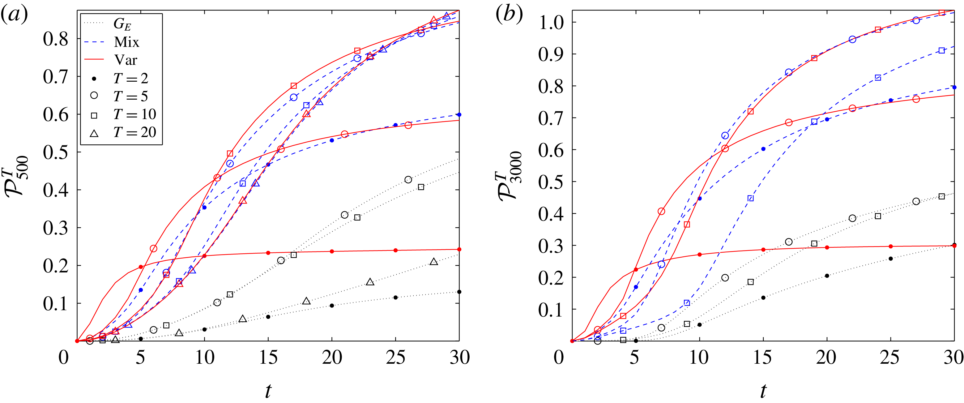
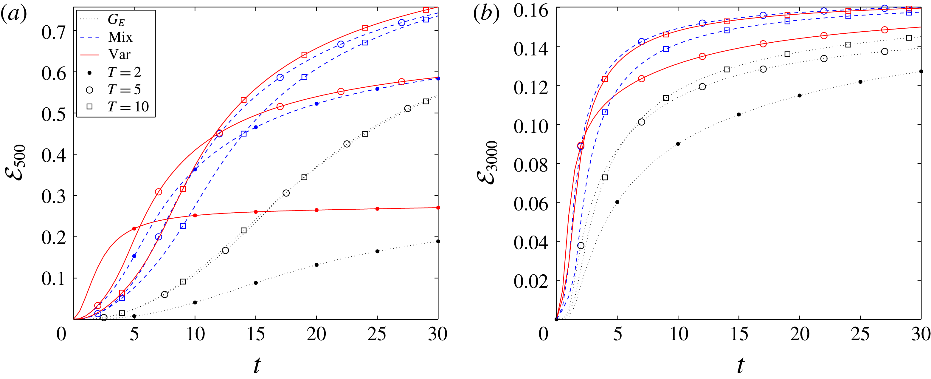
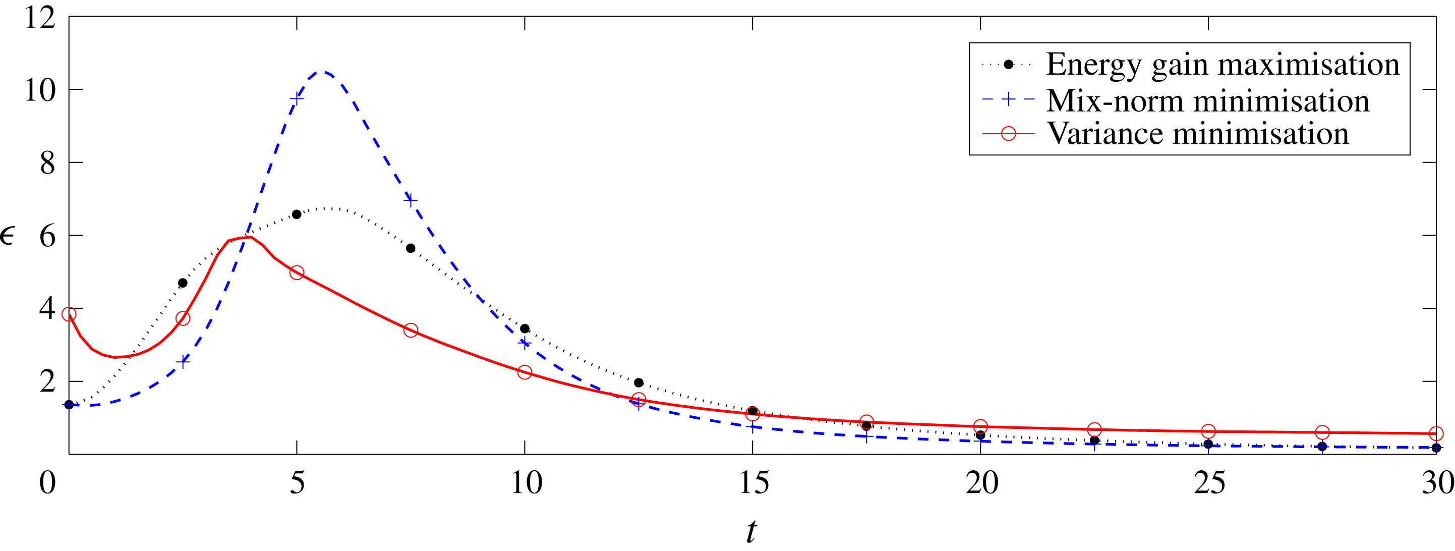
1 Introduction
Understanding the process of fluid mixing is a long-standing challenge in fluid dynamics research. One of the problems that lies at the heart of the study of mixing is the broad concept of ‘efficiency’. For example, what is an optimal mixing strategy that produces, at a given time, the best possible mixture, subject perhaps to some constraints? Here, we wish to address certain aspects of this question by considering a canonical problem: the mixing of a passive scalar with finite diffusivity in plane Poiseuille flow, i.e. the (in general three-dimensional) flow of a fluid with finite viscosity driven by a constant imposed pressure gradient in a finite-depth channel between two horizontal plane boundaries.
The classical picture of scalar mixing of a fluid dates back at least to Eckart (Reference Eckart1948) and Welander (Reference Welander1955). Homogenisation of two initially separated, miscible substances is achieved in two stages. Firstly, the interface between the substances is stretched and folded by an advection field, i.e. the substances are ‘stirred’, resulting in a filamentary structure which both increases the surface area of the interfaces between the two miscible substances, and increases the concentration gradients in the vicinity of those interfaces. Secondly, these interfaces are smeared out due to the action of molecular diffusion, which causes the gradients to decrease and ultimately vanish. However, owing to the wide range of contexts in which such irreversible mixing is actually encountered, there is no general theory available to describe all aspects of the phenomenon. Indeed, even the definition of what constitutes ‘mixing’ is not universally accepted. Analogously to the problem of turbulence, in different contexts, different mathematical descriptions are used as quantitative measures for ‘mixing’.
A commonly used, systematic approach to modelling mixing combines the kinematical foundations of fluid mechanics with the theory of dynamical systems, particularly the concept of chaos (Ottino Reference Ottino1989; Wiggins Reference Wiggins1992). Mixing is thus characterised by some stretching function that measures the ability of the flow to stretch and fold the interfacial area between two initially segregated substances. Starting with Aref’s blinking vortex flow (Aref Reference Aref1984), mixing characteristics of a large number of flows (Ottino Reference Ottino1990) have been assessed using various concepts from the theory of dynamical systems. Such concepts undoubtedly provide valuable insights. Stretching and folding are certainly characteristic of chaos, and efficient mixing is guaranteed if the flow exhibits ‘streamline crossing’, i.e. (loosely) the streamlines of the flow in a bounded domain at two different times must, when projected onto each other, show intersecting streamlines (Wiggins & Ottino Reference Wiggins and Ottino2004). A mathematically precise description of such efficient mixing is captured in the framework of linked twist maps (Sturman, Ottino & Wiggins Reference Sturman, Ottino and Wiggins2006). However, such a description relies on time periodicity of the underlying flows with small perturbations from integrability, and is, by its very nature, principally suited to the study of the long-time behaviour of the system. Therefore, different descriptions and approaches may well be better suited to flows where mixing over finite time horizons is of interest.
For optimisation and control problems, it is practicable (and natural) to measure mixing using the time evolution of various appropriate norms of the scalar miscible quantity’s concentration field, in particular the difference of this concentration from its mean value. A natural candidate is the class of
 $L^{p}$
norms (
 $p\geqslant 1$
), especially the
 $L^{2}$
norm, as it measures the variance of concentration from a completely uniform distribution (Rothstein, Henry & Gollub Reference Rothstein, Henry and Gollub1999; Betz Reference Betz2001; Thiffeault & Childress Reference Thiffeault and Childress2003). However, in the absence of molecular diffusion, for example for the important case of immiscible substances, it is possible to establish that
 $L^{p}$
norms are conserved by the action of an arbitrary incompressible (volume-preserving) flow and so they are, at least in this sense, not suitable for the description of mixing.
To overcome this problem, Mathew, Mezi & Petzold (Reference Mathew, Mezi and Petzold2005) introduced the concept of a particular ‘mix-norm’. Unlike the
 $L^{2}$
norm, which is the square of the (zero-mean) concentration field integrated over the whole space, the mix-norm is constructed as an integral of squared mean concentration taken over a dense set of subsets contained in the whole space. They showed that this particular mix-norm is equivalent to
 $H^{-1/2}$
, i.e. the Sobolev norm with a negative, fractional index of
 $1/2$
, and that it is linked to weak convergence and hence to mixing in an ergodic sense. In Mathew et al. (Reference Mathew, Mezić, Grivopoulos, Vaidya and Petzold2007) the authors used this particular mix-norm to optimise mixing in Stokes flow. Later, Lin, Thiffeault & Doering (Reference Lin, Thiffeault and Doering2011) generalised the concept by showing that all ‘mix-norms’ in the class
 $H^{-s},~s\in \mathbb{R}^{+}$
, share desirable mixing properties and found theoretical bounds on optimal mixing times for various constraints. In particular, the mix-norm with index
 $-1$
was successfully used for stirring optimisation, and Thiffeault (Reference Thiffeault2012) applied it to a source–sink transport problem. As we discuss further below, this particular choice of index has specific computational benefits, and will be the one we consider in this paper.
However, in all these studies, the mixing flow field considered was externally imposed, and did not freely evolve as a solution to the full set of governing equations. Furthermore, in practice, the technical challenge of mixing optimisation is commonly approached through exploiting the inevitable connections between mixing and turbulence (Dimotakis & Catrakis Reference Dimotakis and Catrakis1999; Hinch Reference Hinch1999). As turbulence is fundamentally a chaotic process and chaotic advection is key for mixing, it has become an accepted paradigm that ‘better’ (in some sense) mixing will inevitably follow the underlying flow undergoing a transition to, or remaining in, a turbulent regime. Experimentally, this paradigm has been widely studied and verified (Dimotakis Reference Dimotakis2000). Consequently, in many practical applications, mixing is achieved using techniques that are based on pumping energy into the flow, through mechanisms such as mechanical stirring or jet injections (Aamo & Krstić Reference Aamo and Krstić2003). Such energy injection implicitly relies on triggering turbulence, which is then assumed to accomplish the desired mixing.
The required energy injection may be quite large, however, which inevitably has a cost, which may not always be desirable. For example, Aamo, Krstić & Bewley (Reference Aamo, Krstić and Bewley2003) designed an active boundary feedback control to stabilise plane Poiseuille flow, i.e. the flow of a fluid of finite viscosity driven by a constant pressure gradient in a finite-depth channel between two horizontal boundaries. The authors applied the same structure of input but with the opposite sign. Using this approach, with a relatively small control effort realised through wall blowing and suction, they demonstrated that the flow could be destabilised, which triggered complex turbulent flow patterns and consequently resulted in considerable enhancement of mixing. They then conjectured that flow destabilisation is a good proxy for an ‘optimal’ mixing strategy, and then applied this strategy to several other flows such as three-dimensional pipe flow (Balogh, Aamo & Krstić Reference Balogh, Aamo and Krstić2005), two-dimensional flow past a cylinder (Aamo & Krstić Reference Aamo and Krstić2004) and the magnetohydrodynamic channel flow known as ‘Hartmann’ flow (Luo & Schuster Reference Luo and Schuster2009).
However, it was not established directly by Aamo et al. (Reference Aamo, Krstić and Bewley2003) whether triggering energetic perturbations actually is an optimal mixing strategy. Foures, Caulfield & Schmid (Reference Foures, Caulfield and Schmid2014) investigated this issue in the context of a particularly idealised flow: two-dimensional plane Poiseuille flow. As a demonstration of their theoretical and computational approach, they considered the mixing of a zero-mean passive scalar field with diffusivity
 $\unicode[STIX]{x1D705}$
initially organised into two horizontal layers of different concentration, separated by a relatively thin (diffusive) interface. They considered the flow at a relatively low Reynolds number
 $Re=U_{m}h/\unicode[STIX]{x1D708}=500$
, where
 $U_{m}$
is the maximum speed of the induced parabolic background velocity,
 $\unicode[STIX]{x1D708}$
is the kinematic viscosity of the fluid (chosen to be equal to
 $\unicode[STIX]{x1D705}$
for simplicity) and
 $2h$
is the depth of the channel. At this Reynolds number, the flow did not undergo a transition to turbulence. They used a variational constrained optimisation technique, which we refer to herein as the ‘direct-adjoint-looping’ (DAL) method (see Schmid (Reference Schmid2007), Kerswell, Pringle & Willis (Reference Kerswell, Pringle and Willis2014) and Luchini & Bottaro (Reference Luchini and Bottaro2014) for reviews) to identify three different classes of optimal initial perturbations of fixed (finite) kinetic energy. The three classes are optimal in the sense that, at various target times, they minimised either the variance or the
 $H^{-1}$
mix-norm of the scalar concentration field, or maximised the time-averaged kinetic energy of the perturbation.
Their analysis yielded three main results. First, they found that the perturbations that experience the highest energy growth do not effectively homogenise the distribution of the passive scalar, in particular for relatively long optimisation time horizons. Second, based on direct minimisation of the variance of the concentration field, the authors found that the most mixing-efficient strategy is based on exploiting classical ‘Taylor’ shear dispersion. Taylor (Reference Taylor1953) studied the spreading of a solvent in a pipe flow and showed that the radial diffusion of the tracer is enhanced by the cross-stream variation of the velocity field and that the effect grows stronger in the turbulent regime (Taylor Reference Taylor1954). (It is the strength of the shear stresses within the flow and their favourable orientation with respect to the concentration gradients (Rhines & Young Reference Rhines and Young1983) that controls the rate of mixing, and every efficient mixing strategy needs to exploit it.) Third, they found that the perturbations which minimise the mix-norm over short target times proved to be a better (and more computationally efficient) proxy for the perturbations which minimise the variance over long target times (i.e. the best mixing strategy) than perturbations which minimise the variance over short target times. This last result demonstrates the utility of mix-norm-based analyses for identifying optimal mixing strategies, at least in this highly idealised flow.
It is important to appreciate that the results of Foures et al. (Reference Foures, Caulfield and Schmid2014) were obtained in an inherently two-dimensional flow at a substantially smaller Reynolds number (
 $Re=500$
as opposed to
 $Re=6000$
) compared to the results of Aamo et al. (Reference Aamo, Krstić and Bewley2003). Hence, it is at least plausible that these two differences could explain the qualitatively different conclusions of the two studies, in particular since the flows considered by Foures et al. (Reference Foures, Caulfield and Schmid2014) were always highly ordered. Therefore, the purpose of the research presented here is to generalise the study done by Foures et al. (Reference Foures, Caulfield and Schmid2014) to fully three-dimensional flow and to higher Reynolds number, where more complex behaviour may conceivably occur. This generalisation is carried out in two stages. We first consider three-dimensional flow at the same Reynolds number
 $Re=500$
, and then we consider three-dimensional flow at
 $Re=3000$
, where transition to turbulence is possible, particularly for the chosen amplitude of initial perturbation. Fundamentally, we address the following questions for these two stages (i.e. the potential importance of three-dimensionalisation and transition).
Stage 1. When considering three-dimensional flow at
 $Re=500$
:
(i) Does the mixing strategy based on maximisation of the energetic growth of perturbations remain significantly sub-optimal in three-dimensional flow? Yes. While the strategy which uses energy growth is more efficient in three-dimensional flow than in the previously considered two-dimensional flow of Foures et al. (Reference Foures, Caulfield and Schmid2014), it is still significantly outperformed by a mixing strategy which principally takes advantage of Taylor dispersion (Taylor Reference Taylor1953).
(ii) Are the optimal perturbations more effective at mixing in three-dimensional flow? Yes, not least because the extra spatial dimension allows an additional shear to be produced by advection in the spanwise direction which consequently accelerates the mixing, although, somewhat surprisingly, the differences are relatively small between two-dimensional and three-dimensional flows.
(iii) Is there a structural difference between the optimal mixing strategies in two and three dimensions at
 $Re=500$
? No. The optimal mixing process in three dimensions is really rather similar to that described by Foures et al. (Reference Foures, Caulfield and Schmid2014), with the mixing actually passing through three stages: ‘transport’, ‘dispersion’ and ‘relaxation’. Initially, the interface between the two layers of different scalar concentration is perturbed and transported from the centre of the channel towards the walls (forming a characteristic vertical ‘stripe’ structure) where the shear stress is strong. Later, the interface is ‘dispersed’ due to both perturbation advection and the shear associated with the underlying pressure-driven flow via Taylor dispersion, forming a characteristic ‘chevron’ structure. Finally, the distribution of passive scalar ‘relaxes’ to homogeneity by molecular diffusion. Compared to the previously reported flows restricted to two dimensions, the only difference is that, during the second dispersion stage, the perturbation advection is fully three-dimensional, which allows extra dynamics to take place in the spanwise direction of the flow.
(iv) Is the mixing strategy based on mix-norm minimisation a good proxy for optimal mixing in three-dimensional flows? Yes. Once again, in three-dimensional flow, for short optimisation times the mixing strategy based on minimising the mix-norm yields only mildly sub-optimal results. However, the mix-norm-optimal perturbations are, unlike variance-optimal perturbations, weakly sensitive to the variation of the target optimisation time. Hence, for short optimisation times, the mix-norm-based strategy produces better mixtures at long times than the variance-based strategy. For long optimisation times, we observe, entirely in agreement with Foures et al. (Reference Foures, Caulfield and Schmid2014), that the two strategies become highly consistent.

Stage 2. When considering three-dimensional flow at
 $Re=3000$
:
(i) Does the mixing strategy based on energy growth remain sub-optimal in the transitional flows at
$Re=3000$
? Yes. Regardless of the fact that the amplitude of the energy gain is almost doubled compared to the flow at
$Re=500$
, the most energetic perturbations fail to mix the passive scalar trapped in the boundary layers.(ii) Is there a structural difference in the optimal mixing strategy between flows with
$Re=500$
and
$Re=3000$
? No. The fundamental structure of the optimal mixing process is the same at both Reynolds numbers. It still consists of three stages: transport, dispersion and (diffusive) relaxation. Compared to the
$Re=500$
flow, the only difference in the flow at
$Re=3000$
is that the relative impact on mixing of the perturbation advection compared to Taylor dispersion associated with the background pressure-driven parabolic flow is increased due to the large shear stresses available for mixing in the near-boundary region.(iii) Does the mix-norm minimisation remain a good proxy for optimal mixing in flows with
$Re=3000$
? Yes. The time evolution of the mix-norm closely follows the time evolution of the variance, and the mix-norm-optimal initial perturbations remain weakly dependent (relative to the variance-optimal initial perturbations) on the target time in transitional flows with
$Re=3000$
. Thus, the perturbations that minimise the mix-norm over short time horizons result in higher levels of homogeneity at long times compared to the initial perturbations that minimise variance over short time horizons.(iv) Does transition to turbulence enhance mixing? Unsurprisingly, yes. In either sense of concentration variance minimisation or mix-norm minimisation, flows with
$Re=3000$
lead to smaller values (and thus more homogeneous mixtures) in shorter times than flows with
$Re=500$
.(v) Is turbulent mixing more ‘efficient’ than laminar mixing? The answer to this critical question depends on the precise definition of ‘efficiency’. When quantified in terms of the relative head loss of the flow, mixing at
$Re=3000$
is more efficient than at
$Re=500$
. However, relative to the total mechanical work done by the pressure gradient which drives the fluid through the channel, the turbulent mixing at
$Re=3000$
is significantly less efficient than the essentially laminar mixing at
$Re=500$
, which has non-trivial real-world implications.


To justify and explain the above answers to these key questions, the rest of this paper is organised as follows. In § 2 we define precisely the relevant mixing measures and the governing equations for the flow system we are considering. We also formulate mathematically the problem statement and describe our numerical methodology. In § 3.1 we present our results for the three-dimensional flows with
 $Re=500$
, while in § 3.2 we describe the physical processes underlying three-dimensional ‘optimal’ mixing at
 $Re=500$
. These two sections essentially answer the first ‘stage’ of questions above, i.e. the potential importance of inherently three-dimensional flow. In § 3.3 we discuss the mixing results for the transitional flows with
 $Re=3000$
, while in § 3.4 we assess the various measures of mixing efficiency for the flows at
 $Re=500$
and
 $Re=3000$
, thus answering the second ‘stage’ of questions above, i.e. the potential importance of transitional flow. Finally, we draw our conclusions in § 4.
2 Mathematical formulation
2.1 Mixing measures
Let
 $\unicode[STIX]{x1D703}(\boldsymbol{x},t)$
be the concentration of a passive scalar distributed in a bounded domain
 $\unicode[STIX]{x1D6FA}$
. We assume that the total amount of the scalar in
 $\unicode[STIX]{x1D6FA}$
is conserved, and so we assume that there are no sources or sinks and that the net flux through the boundary
 $\unicode[STIX]{x2202}\unicode[STIX]{x1D6FA}$
is zero. Furthermore, we assume that
 $\unicode[STIX]{x2202}\unicode[STIX]{x1D6FA}$
is sufficiently smooth for all the arguments below to hold true. We wish to quantify mixing, i.e. the level of homogeneity of a mixture represented by
 $\unicode[STIX]{x1D703}(\boldsymbol{x},t)$
. The natural way to do so is to compute the variance
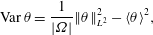 $$\begin{eqnarray}\displaystyle \operatorname{Var}\unicode[STIX]{x1D703}=\frac{1}{|\unicode[STIX]{x1D6FA}|}\Vert \unicode[STIX]{x1D703}\Vert _{L^{2}}^{2}-\langle \unicode[STIX]{x1D703}\rangle ^{2}, & & \displaystyle\end{eqnarray}$$
where
 $$\begin{eqnarray}\displaystyle \Vert \unicode[STIX]{x1D703}\Vert _{L^{2}(\unicode[STIX]{x1D6FA})}^{2}=\int _{\unicode[STIX]{x1D6FA}}\unicode[STIX]{x1D703}^{2}\,\text{d}\boldsymbol{x},\quad \langle \unicode[STIX]{x1D703}\rangle =\frac{1}{|\unicode[STIX]{x1D6FA}|}\int _{\unicode[STIX]{x1D6FA}}\unicode[STIX]{x1D703}\,\text{d}\boldsymbol{x}, & & \displaystyle\end{eqnarray}$$
are the
 $L^{2}$
norm and mean value of
 $\unicode[STIX]{x1D703}$
, respectively, and
 $|\unicode[STIX]{x1D6FA}|$
is the measure of the domain
 $\unicode[STIX]{x1D6FA}$
.
We consider the case where the passive scalar is transported from its initial distribution
 $\unicode[STIX]{x1D703}(\boldsymbol{x},0)=\unicode[STIX]{x1D703}_{0}(\boldsymbol{x})$
by an incompressible flow field
 $\boldsymbol{U}$
(i.e.
 $\unicode[STIX]{x1D735}\boldsymbol{\cdot }\boldsymbol{U}=0$
), such that the spatio-temporal distribution of
 $\unicode[STIX]{x1D703}$
satisfies an advection–diffusion equation, which in non-dimensional form is
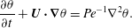 $$\begin{eqnarray}\displaystyle \frac{\unicode[STIX]{x2202}\unicode[STIX]{x1D703}}{\unicode[STIX]{x2202}t}+\boldsymbol{U}\boldsymbol{\cdot }\unicode[STIX]{x1D735}\unicode[STIX]{x1D703}=Pe^{-1}\unicode[STIX]{x1D6FB}^{2}\unicode[STIX]{x1D703}. & & \displaystyle\end{eqnarray}$$
The dimensionless parameter
 $Pe=U_{0}L_{0}/\unicode[STIX]{x1D705}$
is the Péclet number, where
 $U_{0}$
and
 $L_{0}$
are characteristic velocity and length scales of the flow and
 $\unicode[STIX]{x1D705}$
is the diffusion coefficient of the passive scalar in the flow. Without loss of generality we restrict ourselves to zero-mean fields
 $\langle \unicode[STIX]{x1D703}_{0}\rangle =0$
. Application of Stokes’ theorem, along with boundary conditions which impose zero net flux from the domain of interest, yields
 $$\begin{eqnarray}\displaystyle \frac{\,\text{d}}{\,\text{d}t}\langle \unicode[STIX]{x1D703}\rangle =0\quad \text{and}\quad \frac{1}{2}\frac{\,\text{d}}{\,\text{d}t}\Vert \unicode[STIX]{x1D703}\Vert _{L^{2}}^{2}=-Pe^{-1}\Vert \unicode[STIX]{x1D735}\unicode[STIX]{x1D703}\Vert _{L^{2}}^{2}. & & \displaystyle\end{eqnarray}$$
As is well known, the right-hand side in (2.4b
) is strictly negative unless
 $\unicode[STIX]{x1D703}$
is constant, and so the concentration decays with a rate dictated by
 $Pe^{-1}\Vert \unicode[STIX]{x1D735}\unicode[STIX]{x1D703}\Vert _{2}^{2}$
towards the state with
 $\operatorname{Var}\unicode[STIX]{x1D703}=\Vert \unicode[STIX]{x1D703}\Vert _{L^{2}}^{2}=0$
, i.e. the state with uniform distribution of
 $\unicode[STIX]{x1D703}\equiv 0$
. Of course, variance measures the fluctuations of the scalar field from its mean, and in a finite-Péclet-number flow it decays under the action of diffusion until a homogeneous state is reached. The decay rate of variance is proportional to the square of the norm of the concentration gradient, and the velocity field does not appear directly in (2.4). Furthermore, the decay rate is proportional to the inverse of
 $Pe$
, thus suggesting at least the possibility that the rate of change of variance may be small in flows at high Péclet number.
The behaviour of flows at high (yet finite)
 $Pe$
is not immediately clear, however, as the velocity field only influences the evolution of
 $\operatorname{Var}\unicode[STIX]{x1D703}$
through the concentration gradients. Multiplying (2.3) by
 $\unicode[STIX]{x1D6FB}^{2}\unicode[STIX]{x1D703}$
and integrating over
 $\unicode[STIX]{x1D6FA}$
we obtain the evolution equation for the norm of the concentration gradient
 $$\begin{eqnarray}\displaystyle \frac{1}{2}\frac{\,\text{d}}{\,\text{d}t}\Vert \unicode[STIX]{x1D735}\unicode[STIX]{x1D703}\Vert _{L^{2}}^{2}=-\int _{\unicode[STIX]{x1D6FA}}\unicode[STIX]{x1D735}\unicode[STIX]{x1D703}\boldsymbol{\cdot }\boldsymbol{e}\boldsymbol{\cdot }\unicode[STIX]{x1D735}\unicode[STIX]{x1D703}\,\text{d}\boldsymbol{x}-Pe^{-1}\Vert \unicode[STIX]{x1D6FB}^{2}\unicode[STIX]{x1D703}\Vert _{L^{2}}^{2}, & & \displaystyle\end{eqnarray}$$
where
 $\boldsymbol{e}$
is the symmetric part of
 $\unicode[STIX]{x1D735}\boldsymbol{U}$
usually referred to as the rate-of-strain tensor. Equation (2.5) implies that concentration gradients decrease or increase according to their alignment with the principal axes of
 $\boldsymbol{e}$
. The alignment with the negative strain direction increases the concentration gradients and consequently the rate of mixing, while alignment with the positive strain direction has the opposite effect.
Thus, an effective mixing strategy will be one that exploits this fact through promoting the generation and growth of interleaved fluid filaments with high and low concentration. Interfaces between filaments naturally have high concentration gradient and so the growth of such filaments increases mixing transport as diffusion acts on a larger area. If such filamentation is caused by shear in some background flow, such shear-enhanced dispersion is referred to as Taylor dispersion (Taylor Reference Taylor1953), and can substantially increase the ensuing diffusion of the scalar. Crucially, finite-
 $Pe$
flow is fundamentally different from the limiting, yet very important, case when
 $Pe\rightarrow \infty$
, since, in the absence of diffusion, the variance is conserved and
 $\operatorname{Var}\unicode[STIX]{x1D703}(\boldsymbol{x},t)=\operatorname{Var}\unicode[STIX]{x1D703}_{0}$
for any time
 $t$
and any flow field
 $\boldsymbol{U}$
. Hence, in such an idealised flow, variance fails to distinguish between scalar distributions induced by different flows, and so it is not a suitable measure for mixing.
To overcome this disadvantage of variance in the
 $Pe\rightarrow \infty$
limit, various authors have proposed so-called ‘mix-norms’ as measures of mixing. Originally, Mathew et al. (Reference Mathew, Mezi and Petzold2005) proposed to use a norm that is equivalent to the norm associated with a Sobolev space of a negative fractional index
 $H^{-1/2}$
. Subsequently, Thiffeault (Reference Thiffeault2012) showed that a whole class of norms associated with
 $H^{-s}$
,
 $s>0$
, can be used to measure mixing. One mathematical advantage of mix-norms is in their relationship to the ergodic definition of mixing. Here, similarly to Foures et al. (Reference Foures, Caulfield and Schmid2014), we introduce a mix-norm (with negative index
 $-1$
) in the following way, which has certain computational advantages. Consider a function
 $\unicode[STIX]{x1D6E9}$
which is a solution to
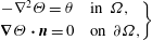 $$\begin{eqnarray}\displaystyle \left.\begin{array}{@{}cl@{}}-\unicode[STIX]{x1D6FB}^{2}\unicode[STIX]{x1D6E9}=\unicode[STIX]{x1D703}\quad & \text{in }\unicode[STIX]{x1D6FA},\\ \unicode[STIX]{x1D735}\unicode[STIX]{x1D6E9}\boldsymbol{\cdot }\boldsymbol{n}=0\quad & \text{on }\unicode[STIX]{x2202}\unicode[STIX]{x1D6FA},\end{array}\right\} & & \displaystyle\end{eqnarray}$$
with the extra condition
 $$\begin{eqnarray}\displaystyle \int _{\unicode[STIX]{x1D6FA}}\unicode[STIX]{x1D6E9}\,\text{d}\boldsymbol{x}=0, & & \displaystyle\end{eqnarray}$$
which guarantees the uniqueness of
 $\unicode[STIX]{x1D6E9}$
. Then, we define our particular mix-norm as
 $$\begin{eqnarray}\displaystyle \operatorname{Mix}\unicode[STIX]{x1D703}=\frac{1}{|\unicode[STIX]{x1D6FA}|}\Vert \unicode[STIX]{x1D735}^{-1}\unicode[STIX]{x1D703}\Vert _{L^{2}(\unicode[STIX]{x1D6FA})}\equiv \frac{1}{|\unicode[STIX]{x1D6FA}|}\Vert \unicode[STIX]{x1D735}\unicode[STIX]{x1D6E9}\Vert _{L^{2}(\unicode[STIX]{x1D6FA})}. & & \displaystyle\end{eqnarray}$$
As we discuss in more detail below, this choice of mix-norm, and the associated choice of the homogeneous Neumann boundary condition in (2.6), naturally arises in our mixing optimisation problem formulation.
In the case when the domain of interest
 $\unicode[STIX]{x1D6FA}$
is a torus, the operator
 $\unicode[STIX]{x1D735}^{-1}$
can be simply expressed in terms of Fourier series. In such a situation, the mix-norm becomes
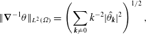 $$\begin{eqnarray}\displaystyle \Vert \unicode[STIX]{x1D735}^{-1}\unicode[STIX]{x1D703}\Vert _{L^{2}(\unicode[STIX]{x1D6FA})}=\left(\mathop{\sum }_{\boldsymbol{k}\neq 0}k^{-2}|\hat{\unicode[STIX]{x1D703}}_{\boldsymbol{k}}|^{2}\right)^{1/2}, & & \displaystyle\end{eqnarray}$$
where
 $\boldsymbol{k}$
is the wavevector with magnitude
 $k$
and
 $\hat{\unicode[STIX]{x1D703}}_{\boldsymbol{k}}$
are the Fourier coefficients of
 $\unicode[STIX]{x1D703}$
. The prefactor
 $k^{-2}$
in (2.9) emphasises large-scale structures (with small
 $k$
) in the flow over small-scale structures (large
 $k$
). Therefore, minimisation of this mix-norm will deprecate large-scale structures, a procedure which is at least intuitively suggestive of encouraging diffusive mixing. Analogously to the derivation of (2.5), multiplying (2.3) by
 $\unicode[STIX]{x1D6E9}$
and integrating over
 $\unicode[STIX]{x1D6FA}$
yields the evolution equation for the mix-norm of the concentration:
 $$\begin{eqnarray}\displaystyle \frac{1}{2}\frac{\,\text{d}}{\,\text{d}t}\Vert \unicode[STIX]{x1D735}^{-1}\unicode[STIX]{x1D703}\Vert _{L^{2}}^{2}=\int _{\unicode[STIX]{x1D6FA}}\unicode[STIX]{x1D735}^{-1}\unicode[STIX]{x1D703}\boldsymbol{\cdot }\boldsymbol{e}\boldsymbol{\cdot }\unicode[STIX]{x1D735}^{-1}\unicode[STIX]{x1D703}\,\text{d}\boldsymbol{x}-Pe^{-1}\Vert \unicode[STIX]{x1D703}\Vert _{L^{2}}^{2}. & & \displaystyle\end{eqnarray}$$
Comparing this equation with (2.5) shows that the velocity gradients affect
 $\Vert \unicode[STIX]{x1D735}^{-1}\unicode[STIX]{x1D703}\Vert _{L^{2}}$
exactly in the opposite way to the way they affect
 $\Vert \unicode[STIX]{x1D735}\unicode[STIX]{x1D703}\Vert _{L^{2}}$
. Crucially, advection which promotes filamentation and hence increases concentration gradients actually generates structures at smaller and smaller scales which inevitably imply decay in the mix-norm. Therefore, minimisation of the mix-norm encourages the same stirring strategy as minimisation of the variance yet, crucially, it does not exhibit the same singular behaviour as
 $Pe\rightarrow \infty$
. Indeed, as already observed for two-dimensional flow by Foures et al. (Reference Foures, Caulfield and Schmid2014), and as we demonstrate for three-dimensional flow below, even for large-
 $Pe$
flow, it is possible for the mix-norm to decrease relatively rapidly for flows particularly conducive to mixing. This rapid decrease is particularly helpful within an iterative procedure designed to identify an ‘optimal’ mixing strategy, and so we believe it is appropriate to consider the mix-norm to be both a mathematically sound and a computationally attractive measure for mixing.
2.2 Governing equations and problem statement
We consider the model problem of mixing a passive scalar by an incompressible flow in a three-dimensional channel, where the flow is driven by a (constant) pressure gradient. The channel is modelled as a three-dimensional domain of streamwise length
 $L^{\ast }=4\unicode[STIX]{x03C0}h^{\ast }$
, spanwise width
 $W^{\ast }=\unicode[STIX]{x03C0}h^{\ast }$
and height
 $H^{\ast }=2h^{\ast }$
. For computational convenience, periodicity is imposed in the streamwise and spanwise directions. Although the associated re-entrant flow of the scalar field at the streamwise and spanwise boundaries is not physical, we are principally interested in demonstrating the utility of the combination of the DAL method and minimisation of the mix-norm as a procedure to identify initial conditions which encourage subsequent efficient scalar mixing, for which this model problem formulation is appropriate.
The divergence-free flow velocity
 $\boldsymbol{U}(\boldsymbol{x},t)$
is governed by the Navier–Stokes equations and the continuity equation, with (total) pressure
 $P(\boldsymbol{x},t)$
imposing incompressibility. As already discussed, the concentration
 $\unicode[STIX]{x1D703}(\boldsymbol{x},t)$
of the passive scalar field satisfies an advection–diffusion equation, and so the non-dimensional evolution is governed by
 $$\begin{eqnarray}\displaystyle & \displaystyle \frac{\unicode[STIX]{x2202}\boldsymbol{U}}{\unicode[STIX]{x2202}t}+\boldsymbol{U}\boldsymbol{\cdot }\unicode[STIX]{x1D735}\boldsymbol{U}=-\unicode[STIX]{x1D735}P+Re^{-1}\unicode[STIX]{x1D6FB}^{2}\boldsymbol{U}, & \displaystyle\end{eqnarray}$$
 $$\begin{eqnarray}\displaystyle & \displaystyle \unicode[STIX]{x1D735}\boldsymbol{\cdot }\boldsymbol{U}=0, & \displaystyle\end{eqnarray}$$
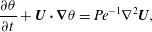 $$\begin{eqnarray}\displaystyle & \displaystyle \frac{\unicode[STIX]{x2202}\unicode[STIX]{x1D703}}{\unicode[STIX]{x2202}t}+\boldsymbol{U}\boldsymbol{\cdot }\unicode[STIX]{x1D735}\unicode[STIX]{x1D703}=Pe^{-1}\unicode[STIX]{x1D6FB}^{2}\boldsymbol{U}, & \displaystyle\end{eqnarray}$$
where all lengths are scaled by the channel half-depth
 $h^{\ast }$
, velocities are scaled by the (dimensional) maximum centreline velocity
 $U_{m}^{\ast }$
and times are scaled by
 $\unicode[STIX]{x1D70F}^{\ast }=h^{\ast }/U_{m}^{\ast }$
. (Hence the non-dimensional domain size is
 $[0,4\unicode[STIX]{x03C0}]\times [-1,1]\times [0,\unicode[STIX]{x03C0}]$
.) The system is naturally characterised by two non-dimensional numbers, the Reynolds number
 $Re$
and the Péclet number
 $Pe$
, defined as
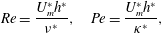 $$\begin{eqnarray}\displaystyle Re=\frac{U_{m}^{\ast }h^{\ast }}{\unicode[STIX]{x1D708}^{\ast }},\quad Pe=\frac{U_{m}^{\ast }h^{\ast }}{\unicode[STIX]{x1D705}^{\ast }}, & & \displaystyle\end{eqnarray}$$
where
 $\unicode[STIX]{x1D708}^{\ast }$
is the kinematic viscosity and
 $\unicode[STIX]{x1D705}^{\ast }$
is the scalar field diffusivity, respectively. Here, for simplicity, we set
 $Re=Pe$
, and so the Schmidt number
 $Sc=\unicode[STIX]{x1D708}^{\ast }/\unicode[STIX]{x1D705}^{\ast }=1$
. It is important to remember that we consider a passive scalar field: in the system (2.11)–(2.13) the flow is independent of the concentration field
 $\unicode[STIX]{x1D703}(\boldsymbol{x},t)$
. Therefore, we can solve (2.11) and (2.12) separately and let the concentration field evolve from its initial distribution
 $\unicode[STIX]{x1D703}_{0}=\unicode[STIX]{x1D703}(\boldsymbol{x},0)$
under the action of
 $\boldsymbol{U}$
in (2.13).
Assuming that the flow is driven by a constant pressure gradient
 $\text{d}\bar{p}^{\ast }/\text{d}x^{\ast }$
, the system (2.11)–(2.12) admits a steady base flow solution
 $$\begin{eqnarray}\displaystyle \bar{\boldsymbol{u}}=(1-y^{2})\boldsymbol{e}_{\boldsymbol{x}}, & & \displaystyle\end{eqnarray}$$
where
 $y$
is the wall-normal coordinate and
 $\boldsymbol{e}_{\boldsymbol{x}}$
is the unit vector in the (streamwise)
 $x$
-direction. Hence, the characteristic velocity
 $u_{c}^{\ast }$
and the pressure gradient are related by
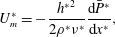 $$\begin{eqnarray}\displaystyle U_{m}^{\ast }=-\frac{{h^{\ast }}^{2}}{2\unicode[STIX]{x1D70C}^{\ast }\unicode[STIX]{x1D708}^{\ast }}\frac{\text{d}\bar{P}^{\ast }}{\text{d}x^{\ast }}, & & \displaystyle\end{eqnarray}$$
where
 $\unicode[STIX]{x1D70C}^{\ast }$
is the (constant) fluid density. Therefore, the non-dimensional pressure gradient is given by
 $2/Re=-\text{d}\bar{p}/\text{d}x$
.
Generalising the approach of Foures et al. (Reference Foures, Caulfield and Schmid2014) to three-dimensional flow, we consider a perturbation velocity
 $\boldsymbol{u}$
with associated perturbation pressure
 $p$
to the base flow
 $\bar{\boldsymbol{u}}$
. This perturbation, in general allowed to be of finite amplitude, then evolves in time satisfying
 $$\begin{eqnarray}\displaystyle & \displaystyle \frac{\unicode[STIX]{x2202}\boldsymbol{u}}{\unicode[STIX]{x2202}t}+\boldsymbol{U}\boldsymbol{\cdot }\unicode[STIX]{x1D735}\boldsymbol{u}+\boldsymbol{u}\boldsymbol{\cdot }\unicode[STIX]{x1D735}\bar{\boldsymbol{u}}=-\unicode[STIX]{x1D735}p+Re^{-1}\unicode[STIX]{x1D6FB}^{2}\boldsymbol{u}, & \displaystyle\end{eqnarray}$$
 $$\begin{eqnarray}\displaystyle & \displaystyle \unicode[STIX]{x1D735}\boldsymbol{\cdot }\boldsymbol{u}=0, & \displaystyle\end{eqnarray}$$
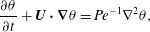 $$\begin{eqnarray}\displaystyle & \displaystyle \frac{\unicode[STIX]{x2202}\unicode[STIX]{x1D703}}{\unicode[STIX]{x2202}t}+\boldsymbol{U}\boldsymbol{\cdot }\unicode[STIX]{x1D735}\unicode[STIX]{x1D703}=Pe^{-1}\unicode[STIX]{x1D6FB}^{2}\unicode[STIX]{x1D703}, & \displaystyle\end{eqnarray}$$
where the total velocity field
 $\boldsymbol{U}=\bar{\boldsymbol{u}}+\boldsymbol{u}$
and the total pressure
 $P=\bar{p}+p$
. As already noted, we impose periodic boundary conditions in the streamwise
 $x$
-direction and spanwise
 $z$
-direction. We also impose
 $$\begin{eqnarray}\displaystyle \boldsymbol{u}=0,\quad \frac{\unicode[STIX]{x2202}p}{\unicode[STIX]{x2202}y}=0,\quad \frac{\unicode[STIX]{x2202}\unicode[STIX]{x1D703}}{\unicode[STIX]{x2202}y}=0\quad \text{on }\unicode[STIX]{x1D6E4}, & & \displaystyle\end{eqnarray}$$
where
 $\unicode[STIX]{x1D6E4}$
denotes the plane channel walls at
 $y=\pm 1$
. Finally, we prescribe the initial conditions
 $$\begin{eqnarray}\displaystyle \boldsymbol{u}(\boldsymbol{x},0)=\boldsymbol{u}_{0}(\boldsymbol{x})\quad \text{and}\quad \unicode[STIX]{x1D703}(\boldsymbol{x},0)=\unicode[STIX]{x1D703}_{0}(\boldsymbol{x}). & & \displaystyle\end{eqnarray}$$
In our problems of interest,
 $\boldsymbol{u}_{0}$
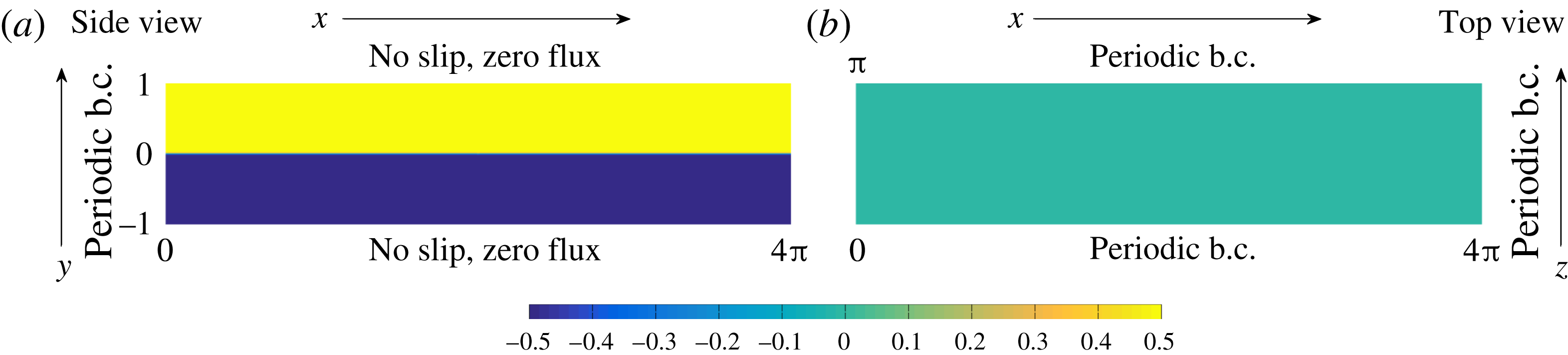
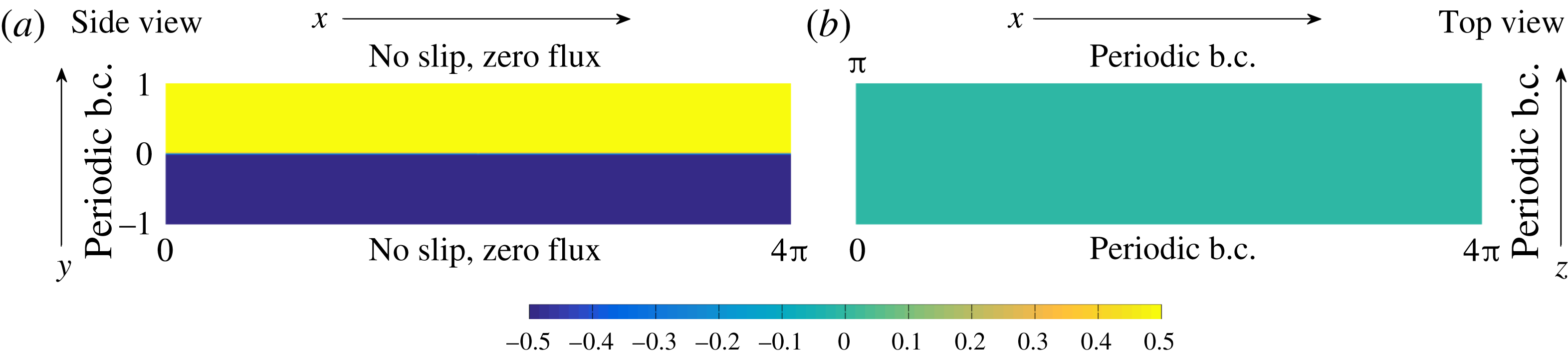
is our control variable. The scalar field is initially organised into two layers, one of high and one of low concentration, as shown schematically in figure 1. We assume that there is an approximately diffusive interface between these two layers, such that
 $$\begin{eqnarray}\displaystyle \unicode[STIX]{x1D703}_{0}(\boldsymbol{x})={\textstyle \frac{1}{2}}\tanh (Cy), & & \displaystyle\end{eqnarray}$$
where the parameter
 $C$
is chosen so that the interface is both ‘sharp’, and yet adequately resolved numerically. By resolution tests, we find that
 $C=30$
is an appropriate choice, although the particular choice of this parameter does not have a significant effect on our results.
We consider such a streamwise-independent and spanwise-independent initial distribution, as it is not modified by the steady base flow solution (2.15), varying only due to diffusion. We choose this initial distribution as we are interested in identifying initial perturbations in the velocity field that lead to enhanced mixing by some target time. This is qualitatively different from the class of problems that seek to identify initial density distributions, in general non-trivially varying in all spatial directions, which lead to enhanced mixing by some target time (see for example Farazmand (Reference Farazmand2017) and references therein). In principle such a class of problems could also be formulated using the DAL method discussed below, but we do not consider this class further here for clarity, as we wish to focus on the mixing effectiveness of initial velocity perturbations with a certain (constrained) kinetic energy.
We denote by
 ${\mathcal{N}}{\mathcal{S}}_{u_{0}}^{div}$
the family of solutions to the incompressible Navier–Stokes equations (2.17) and (2.18) with boundary conditions defined in (2.20) and initial condition
 $\boldsymbol{u}_{0}$
. Analogously, we denote by
 ${\mathcal{A}}{\mathcal{D}}_{\unicode[STIX]{x1D703}_{0}}$
the family of solutions to (2.19) and (2.20) with initial scalar distribution (2.22). Our objective is then to identify an initial perturbation
 $\boldsymbol{u}_{0}$
to the base flow
 $\bar{\boldsymbol{u}}$
which leads, through flow evolution as a solution to the system (2.17)–(2.22), to an ‘optimal’ measure (for example the variance or mix-norm as introduced above in (2.8)) of mixing when evaluated at some time horizon
 $T$
.
It is natural to expect that the magnitude of this initial perturbation is significant, and so we constrain the kinetic energy of the initial condition,
 $$\begin{eqnarray}\displaystyle \Vert \boldsymbol{u}_{0}(\boldsymbol{x})\Vert _{L^{2}(\unicode[STIX]{x1D6FA})}^{2}=2e_{0}|\unicode[STIX]{x1D6FA}|, & & \displaystyle\end{eqnarray}$$
where
 $e_{0}$
is the energy density and
 $|\unicode[STIX]{x1D6FA}|$
is the volume of our flow domain. It seems highly plausible that growth in the energy of the perturbation to the base flow will lead to mixing, and so Aamo & Krstić (Reference Aamo and Krstić2003) proposed to use the perturbations that most strongly destabilise the base flow to enhance mixing. However, in the two-dimensional analogue of the flow considered here, Foures et al. (Reference Foures, Caulfield and Schmid2014) did not find that such perturbations led to the most mixing (as measured by small values of the variance at the time horizon), although they only considered a flow with
 $Re=500$
, which did not exhibit vigorous disordered motion, presumably both because the Reynolds number was too low, and because of the restriction to two dimensions. We wish to test this conjecture in more realistic three-dimensional (and higher-Reynolds-number) flows through quantifying the amount of mixing caused by a perturbation that maximises the energy growth in the perturbation. Therefore, as well as considering values of the variance and the mix-norm at the target time, we consider also the time-integrated (perturbation kinetic) energy growth over the entire time interval
 $[0,T]$
of a perturbation
 $\boldsymbol{u}$
, defined as
 $$\begin{eqnarray}\displaystyle G_{E}(T)=\frac{1}{2}\int _{0}^{T}\Vert \boldsymbol{u}(\boldsymbol{x},\unicode[STIX]{x1D70F})\Vert _{L^{2}(\unicode[STIX]{x1D6FA})}^{2}\,\text{d}\unicode[STIX]{x1D70F}. & & \displaystyle\end{eqnarray}$$
As discussed in more detail in Foures et al. (Reference Foures, Caulfield and Schmid2014), we examine the time-integrated energy growth, rather than only the energy of the perturbation at the target time
 $T$
, because such time integration captures perturbations which exhibit transient growth during the time interval of interest. Such perturbations may not necessarily have maximum amplitude precisely at the target time
 $T$
, yet may have substantially larger peak amplitude (occurring at
 $t_{p}<T$
) and potentially substantially more mixing than the transiently growing perturbation with peak amplitude occurring at
 $T$
.
Schematic representation of the initial distribution and boundary conditions imposed on the scalar concentration field shown in (a) side view on the midplane
 $z=\unicode[STIX]{x03C0}/2$
and (b) top view on the midplane
 $y=0$
.
Defining our problem(s) of interest formally, we adopt a slight modification of the notation used by Foures et al. (Reference Foures, Caulfield and Schmid2014). We define the objective functional
 $$\begin{eqnarray}\displaystyle {\mathcal{J}}(\boldsymbol{u}(T),\unicode[STIX]{x1D703}(T))=-\frac{1-\unicode[STIX]{x1D6FC}}{2}\int _{0}^{T}\Vert \boldsymbol{u}(\boldsymbol{x},t)\Vert _{L^{2}(\unicode[STIX]{x1D6FA})}^{2}\,\text{d}t+\frac{\unicode[STIX]{x1D6FC}}{2}\Vert \unicode[STIX]{x1D735}^{-\unicode[STIX]{x1D6FD}}\unicode[STIX]{x1D703}(\boldsymbol{x},T)\Vert _{L^{2}(\unicode[STIX]{x1D6FA})}^{2}, & & \displaystyle\end{eqnarray}$$
where the parameters
 $\unicode[STIX]{x1D6FC}\in \{0,1\}$
and
 $\unicode[STIX]{x1D6FD}\in \{0,1\}$
. Choosing
 $\unicode[STIX]{x1D6FC}=0$
corresponds to considering the time-averaged energy; choosing
 $\unicode[STIX]{x1D6FC}=1,~\unicode[STIX]{x1D6FD}=0$
corresponds to considering the variance; and choosing
 $\unicode[STIX]{x1D6FC}=1,~\unicode[STIX]{x1D6FD}=1$
corresponds to considering the mix-norm. For these various choices of these parameters, we then solve the minimisation problem
 $$\begin{eqnarray}\displaystyle \underset{\Vert \boldsymbol{u}_{0}\Vert _{L^{2}}^{2}=2e_{0}|\unicode[STIX]{x1D6FA}|}{\operatorname{argmin}}\{{\mathcal{J}}(\boldsymbol{u}(T),\unicode[STIX]{x1D703}(T))\mid (\boldsymbol{u},\unicode[STIX]{x1D703})\in {\mathcal{N}}{\mathcal{S}}_{u_{0}}^{div}\times {\mathcal{A}}{\mathcal{D}}_{\unicode[STIX]{x1D703}_{0}}\}. & & \displaystyle\end{eqnarray}$$
2.3 Direct-adjoint-looping method
The central challenge of the problem (2.26) is due to the fact that the objective functional
 ${\mathcal{J}}$
does not depend explicitly on the control variable
 $\boldsymbol{u}_{0}$
. Instead, the control affects
 ${\mathcal{J}}$
through the effect that the choice of this initial condition has on the spatially and temporally varying velocity fields and concentration fields, which are constrained to satisfy their evolution equations (2.17)–(2.19), and associated boundary conditions (2.20). These constraints need to be included in the objective functional using additional spatially and temporally varying ‘adjoint’ variables. Then, the variation of
 ${\mathcal{J}}$
with respect to the control variable
 $\boldsymbol{u}_{0}$
may be derived and a classical gradient-based optimisation approach can be employed. Such a strategy to tackle the minimisation problem (2.26) is sometimes referred to as a (nonlinear) direct-adjoint looping (DAL) method (Kerswell et al.
Reference Kerswell, Pringle and Willis2014; Luchini & Bottaro Reference Luchini and Bottaro2014). As discussed in detail in these reviews, this method has become increasingly popular recently, particularly in terms of identifying finite-amplitude perturbations, and the associated hierarchy of growth mechanisms, which optimise energy gain over finite time horizons, and indeed may trigger the transition to turbulence (see for example Cherubini et al.
Reference Cherubini, De Palma, Robinet and Bottaro2010; Pringle & Kerswell Reference Pringle and Kerswell2010; Juniper Reference Juniper2011; Monokrousos et al.
Reference Monokrousos, Bottaro, Brandt, Di Vita and Henningson2011; Pringle, Willis & Kerswell Reference Pringle, Willis and Kerswell2012; Rabin, Caulfield & Kerswell Reference Rabin, Caulfield and Kerswell2012; Duguet et al.
Reference Duguet, Monokrousos, Brandt and Henningson2013).
However, the method is quite general, and Foures et al. (Reference Foures, Caulfield and Schmid2014) demonstrated that it could be applied to the identification of initial perturbations (and indeed forcing strategies) which lead to ‘optimal’ mixing, in various (well-defined) mathematical senses. Following the implementation of this method presented in Foures et al. (Reference Foures, Caulfield and Schmid2014), repeated briefly here for completeness, we introduce ‘adjoint’ variables
 $\boldsymbol{u}_{0}^{\dagger }$
,
 $\boldsymbol{u}^{\dagger }$
,
 $\unicode[STIX]{x1D703}^{\dagger }$
and
 $p^{\dagger }$
and consider the augmented functional
 $$\begin{eqnarray}\displaystyle {\mathcal{L}}(\boldsymbol{u}_{0},\boldsymbol{u},\unicode[STIX]{x1D703},p,\boldsymbol{u}_{0}^{\dagger },\boldsymbol{u}^{\dagger },\unicode[STIX]{x1D703}^{\dagger },p^{\dagger }) & = & \displaystyle {\mathcal{J}}(\boldsymbol{u}(T),\unicode[STIX]{x1D703}(T))-{\mathcal{J}}_{{\mathcal{N}}{\mathcal{S}}}(\boldsymbol{u},p,\boldsymbol{u}^{\dagger })-{\mathcal{J}}_{{\mathcal{A}}{\mathcal{D}}}(\unicode[STIX]{x1D703}^{\dagger },\unicode[STIX]{x1D703},\boldsymbol{u})\nonumber\\ \displaystyle & & \displaystyle -\,{\mathcal{J}}_{{\mathcal{C}}}(p^{\dagger },\boldsymbol{u})-{\mathcal{J}}_{{\mathcal{I}}{\mathcal{C}}}(\boldsymbol{u}_{0},\boldsymbol{u},\boldsymbol{u}_{0}^{\dagger }),\end{eqnarray}$$
where
 $$\begin{eqnarray}\displaystyle & \displaystyle {\mathcal{J}}_{{\mathcal{N}}{\mathcal{S}}}=\int _{0}^{T}\!\!\int _{\unicode[STIX]{x1D6FA}}\boldsymbol{u}^{\dagger }\boldsymbol{\cdot }\left(\frac{\unicode[STIX]{x2202}\boldsymbol{u}}{\unicode[STIX]{x2202}t}+\boldsymbol{U}\boldsymbol{\cdot }\unicode[STIX]{x1D735}\boldsymbol{u}+\boldsymbol{u}\boldsymbol{\cdot }\unicode[STIX]{x1D735}\bar{\boldsymbol{u}}+\unicode[STIX]{x1D735}p-Re^{-1}\unicode[STIX]{x1D6FB}^{2}\boldsymbol{u}\right)\,\text{d}\boldsymbol{x}\,\text{d}t, & \displaystyle\end{eqnarray}$$
 $$\begin{eqnarray}\displaystyle & \displaystyle {\mathcal{J}}_{{\mathcal{A}}{\mathcal{D}}}=\int _{0}^{T}\!\!\int _{\unicode[STIX]{x1D6FA}}\unicode[STIX]{x1D703}^{\dagger }\left(\frac{\unicode[STIX]{x2202}\unicode[STIX]{x1D703}}{\unicode[STIX]{x2202}t}+\boldsymbol{U}\boldsymbol{\cdot }\unicode[STIX]{x1D735}\unicode[STIX]{x1D703}-Pe^{-1}\unicode[STIX]{x1D6FB}^{2}\unicode[STIX]{x1D703}\right)\,\text{d}\boldsymbol{x}\,\text{d}t, & \displaystyle\end{eqnarray}$$
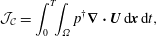 $$\begin{eqnarray}\displaystyle & \displaystyle {\mathcal{J}}_{{\mathcal{C}}}=\int _{0}^{T}\!\!\int _{\unicode[STIX]{x1D6FA}}p^{\dagger }\unicode[STIX]{x1D735}\boldsymbol{\cdot }\boldsymbol{U}\,\text{d}\boldsymbol{x}\,\text{d}t, & \displaystyle\end{eqnarray}$$
 $$\begin{eqnarray}\displaystyle & \displaystyle {\mathcal{J}}_{{\mathcal{I}}{\mathcal{C}}}=\int _{\unicode[STIX]{x1D6FA}}\boldsymbol{u}_{0}^{\dagger }\boldsymbol{\cdot }(\boldsymbol{u}(\boldsymbol{x},0)-\boldsymbol{u}_{0})\,\text{d}\boldsymbol{x}. & \displaystyle\end{eqnarray}$$
The minimisers of (2.27) are characterised by vanishing Gateaux derivatives,
 $\unicode[STIX]{x1D6FF}_{G}{\mathcal{L}}=0$
. Naturally, variation of
 ${\mathcal{L}}$
with respect to the adjoint variables enforces that
 $\boldsymbol{u}$
,
 $\unicode[STIX]{x1D703}$
and
 $p$
satisfy the governing equations (2.17)–(2.19) for
 $t\in [0,T]$
and so the adjoint variables can be regarded as Lagrange multipliers.
Conversely, zero variation of
 ${\mathcal{L}}$
with respect to the ‘forward’ or ‘direct’ variables
 $\boldsymbol{u}$
,
 $p$
and
 $\unicode[STIX]{x1D703}$
implies dynamical constraints which the adjoint variables satisfy at the minimum of
 ${\mathcal{L}}$
. We present the full computation in appendix A, leading to the following set of (adjoint) evolution equations satisfied by the adjoint variables:
 $$\begin{eqnarray}\displaystyle & \displaystyle \frac{\unicode[STIX]{x2202}\boldsymbol{u}^{\dagger }}{\unicode[STIX]{x2202}t}+\boldsymbol{U}\boldsymbol{\cdot }\unicode[STIX]{x1D735}\boldsymbol{u}^{\dagger }-\boldsymbol{u}^{\dagger }\boldsymbol{\cdot }(\unicode[STIX]{x1D735}\boldsymbol{U})^{\text{T}}+\unicode[STIX]{x1D735}p^{\dagger }+Re^{-1}\unicode[STIX]{x1D6FB}^{2}\boldsymbol{u}^{\dagger }=\unicode[STIX]{x1D703}^{\dagger }\unicode[STIX]{x1D735}\unicode[STIX]{x1D703}-(1-\unicode[STIX]{x1D6FC})\boldsymbol{u},\qquad & \displaystyle\end{eqnarray}$$
 $$\begin{eqnarray}\displaystyle & \displaystyle \unicode[STIX]{x1D735}\boldsymbol{\cdot }\boldsymbol{u}^{\dagger }=0, & \displaystyle\end{eqnarray}$$
 $$\begin{eqnarray}\displaystyle & \displaystyle \frac{\unicode[STIX]{x2202}\unicode[STIX]{x1D703}^{\dagger }}{\unicode[STIX]{x2202}t}+\boldsymbol{U}\boldsymbol{\cdot }\unicode[STIX]{x1D735}\unicode[STIX]{x1D703}^{\dagger }+Pe^{-1}\unicode[STIX]{x1D6FB}^{2}\unicode[STIX]{x1D703}^{\dagger }=0, & \displaystyle\end{eqnarray}$$
subject to the boundary conditions
 $$\begin{eqnarray}\displaystyle \boldsymbol{u}^{\dagger }=0,\quad \frac{\unicode[STIX]{x2202}p^{\dagger }}{\unicode[STIX]{x2202}y}=0,\quad \frac{\unicode[STIX]{x2202}\unicode[STIX]{x1D703}^{\dagger }}{\unicode[STIX]{x2202}y}=0\quad \text{at}~\unicode[STIX]{x1D6E4}, & & \displaystyle\end{eqnarray}$$
and terminal conditions
 $$\begin{eqnarray}\displaystyle \boldsymbol{u}^{\dagger }(\boldsymbol{x},T)=0,\quad \unicode[STIX]{x1D703}^{\dagger }(\boldsymbol{x},T)=(-1)^{\unicode[STIX]{x1D6FD}}\unicode[STIX]{x1D6FC}\unicode[STIX]{x1D735}^{-2\unicode[STIX]{x1D6FD}}\unicode[STIX]{x1D703}(\boldsymbol{x},T). & & \displaystyle\end{eqnarray}$$
Finally, for
 $t=0$
we obtain the compatibility conditions
 $$\begin{eqnarray}\displaystyle \boldsymbol{u}_{0}^{\dagger }(\boldsymbol{x})=\boldsymbol{u}^{\dagger }(\boldsymbol{x},0)\quad \text{and}\quad \unicode[STIX]{x1D735}_{\boldsymbol{u}_{0}}{\mathcal{L}}=\boldsymbol{u}_{0}^{\dagger }. & & \displaystyle\end{eqnarray}$$
We can thus set up an iterative ‘looping’ scheme that at each iteration computes the variation of the objective function with respect to
 $\boldsymbol{u}_{0}$
consistently with the imposed constraints, which integrates the direct equations forward in time from 0 to the target time
 $T$
, imposes the terminal conditions on the adjoint variables, and then integrates those variables backwards in time from
 $T$
to 0. Remembering that
 $\boldsymbol{U}=\bar{\boldsymbol{u}}+\boldsymbol{u}$
, the direct disturbance velocity field
 $\boldsymbol{u}$
explicitly appears in the adjoint equation (2.32). Therefore, the velocity field must be saved during the direct time integration so that it can be input into the adjoint evolution equation during the backwards-in-time integration from
 $T$
to 0. Owing to memory constraints, we adopt a classical check-pointing approach in order to avoid saving the direct velocity field at every iteration.
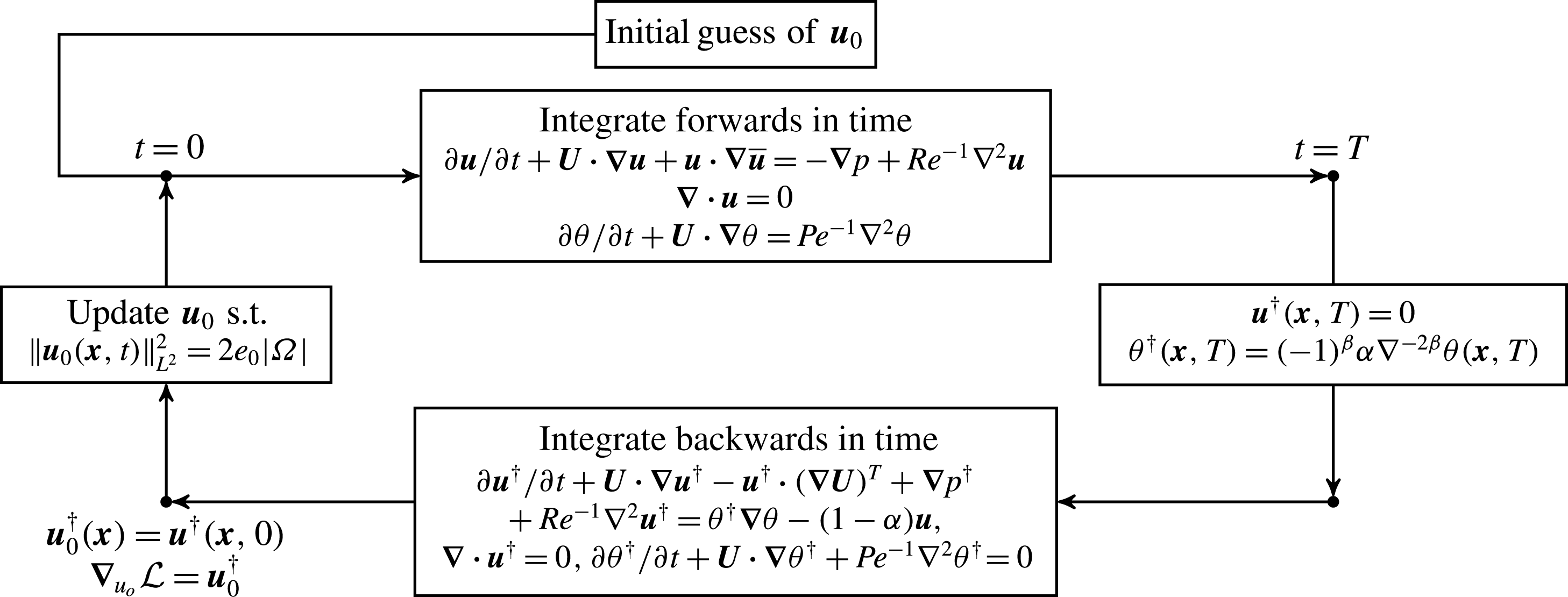
Schematic of the (nonlinear) DAL method for solving the constrained optimisation problem (2.26). At each iteration, the ‘direct’ system (2.17)–(2.19) is integrated forwards in time to the time horizon
 $T$
, where the adjoint variables are initialised and the adjoint system (2.32)–(2.34) is then integrated backwards in time to
 $t=0$
in order to obtain
 $\unicode[STIX]{x1D735}_{\boldsymbol{u}_{0}}{\mathcal{L}}$
. The initial condition is then updated via the conjugate-gradient method combined with a projection step ensuring (2.23) (as described in Foures, Caulfield & Schmid (Reference Foures, Caulfield and Schmid2013)) until convergence.
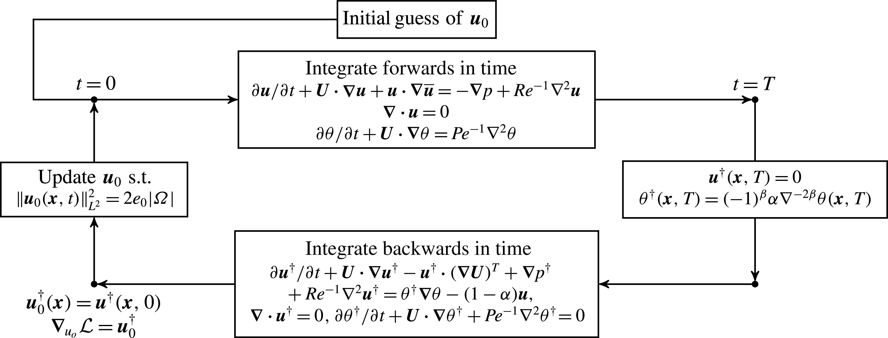
At the first iteration, we start with random (incompressible) noise as an initial guess of the initial perturbation
 $\boldsymbol{u}_{0}$
. The perturbation is evolved forwards in time using the direct governing equations (2.17)–(2.19) until
 $t=T$
. At the time horizon
 $T$
, the adjoint variables are initialised using the terminal conditions (2.36), and the equations (2.32)–(2.34) are integrated backwards in time to
 $t=0$
, as (2.32) is only well-posed when integrating backwards in time. Finally, the gradient of
 ${\mathcal{L}}$
is found and the initial perturbation is updated such that the energy constraint (2.23) is satisfied. We present schematically this DAL method in figure 2. The numerical solver is based upon the well-validated pseudo-spectral code Diablo (see Taylor (Reference Taylor2008) for more details), which uses a combination of the explicit third-order Runge–Kutta–Wray and the implicit Crank–Nicolson schemes for time stepping of the evolution equation. The fractional step method is used to accommodate the incompressibility condition. All derivatives in the periodic directions are computed in Fourier space, while the derivatives in the wall-normal direction are computed via second-order finite differences. We use
 $256\times 209\times 64$
grid points for the spatial discretisation. The time step is chosen to satisfy the classical Courant–Friedrichs–Lewy (CFL) condition which in practice yields
 $\unicode[STIX]{x0394}t\sim 10^{-3}$
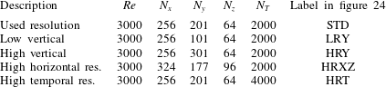
. With the chosen grid density, we observe that the obtained results are not sensitive to the increase of the resolution in either space or time. More details on resolution sensitivity and the convergence properties are given in appendix B.
As discussed in detail in Foures et al. (Reference Foures, Caulfield and Schmid2013), the update of the initial perturbation that respects the energy constraint (2.23) is numerically delicate, and it is convenient to impose this energy constraint directly, rather than using a Lagrange multiplier approach. Imposing this constraint is carried out in two steps. First, once
 $\unicode[STIX]{x1D735}_{\boldsymbol{u}_{0}}{\mathcal{L}}$
is computed, the gradient is projected onto a hyperplane tangent to the energy hypersurface given by (2.23). This is achieved via removal of the hypersurface-normal component
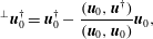 $$\begin{eqnarray}\displaystyle \text{}^{\bot }\boldsymbol{u}_{0}^{\dagger }=\boldsymbol{u}_{0}^{\dagger }-\frac{(\boldsymbol{u}_{0},\boldsymbol{u}^{\dagger })}{(\boldsymbol{u}_{0},\boldsymbol{u}_{0})}\boldsymbol{u}_{0}, & & \displaystyle\end{eqnarray}$$
where
 $(\cdot \,,\cdot )$
represents the standard scalar product in
 $L^{2}$
and the symbol
 $\text{}^{\bot }\boldsymbol{u}_{0}^{\dagger }$
denotes the projection. The update of the initial perturbation is then chosen as
 $$\begin{eqnarray}\displaystyle \boldsymbol{u}_{0}^{new}=\boldsymbol{u}_{0}\cos \unicode[STIX]{x1D6FC}+\boldsymbol{v}\sin \unicode[STIX]{x1D6FC},\quad \text{with }\boldsymbol{v}=2e_{0}|\unicode[STIX]{x1D6FA}|\frac{\text{}^{\bot }\boldsymbol{u}_{0}^{\dagger }}{\Vert \text{}^{\bot }\boldsymbol{u}_{0}^{\dagger }\Vert _{L^{2}}}. & & \displaystyle\end{eqnarray}$$
The energy constraint is imposed directly, via the form of
 $\boldsymbol{v}$
, to restrict the initial perturbation to a hypersphere of given radius, consistently with the direction implied by the projection onto the tangent hyperplane. Geometrically, the update can be interpreted as a rotation of the initial condition in an optimal direction, computed from
 $\unicode[STIX]{x1D735}_{\boldsymbol{u}_{0}}{\mathcal{L}}$
(Douglas, Amari & Kung Reference Douglas, Amari and Kung1998). The angle of the rotation
 $\unicode[STIX]{x1D6FC}$
is an unrestricted parameter and it is determined using classical backtracking line search (Dennis & Schnabel Reference Dennis and Schnabel1996). It is advantageous to use the projection and rotation along with a more advanced gradient-based minimisation algorithm such as the conjugate-gradient descent method (Polak Reference Polak1971), which forms the second stage of the update process.
From the compatibility condition (2.37), convergence to an optimal solution corresponds to
 $\boldsymbol{u}_{0}^{\dagger }$
being computed to be parallel to
 $\boldsymbol{u}_{0}$
, as then
 $\unicode[STIX]{x1D735}_{\boldsymbol{u}_{0}}{\mathcal{L}}=\boldsymbol{u}_{0}^{\dagger }$
can only vary by changing the magnitude of
 $\boldsymbol{u}_{0}$
and hence the energy of the initial perturbation, which is not allowed by construction. This ensures that an (at least local) solution to the minimisation problem (2.26) has been determined.
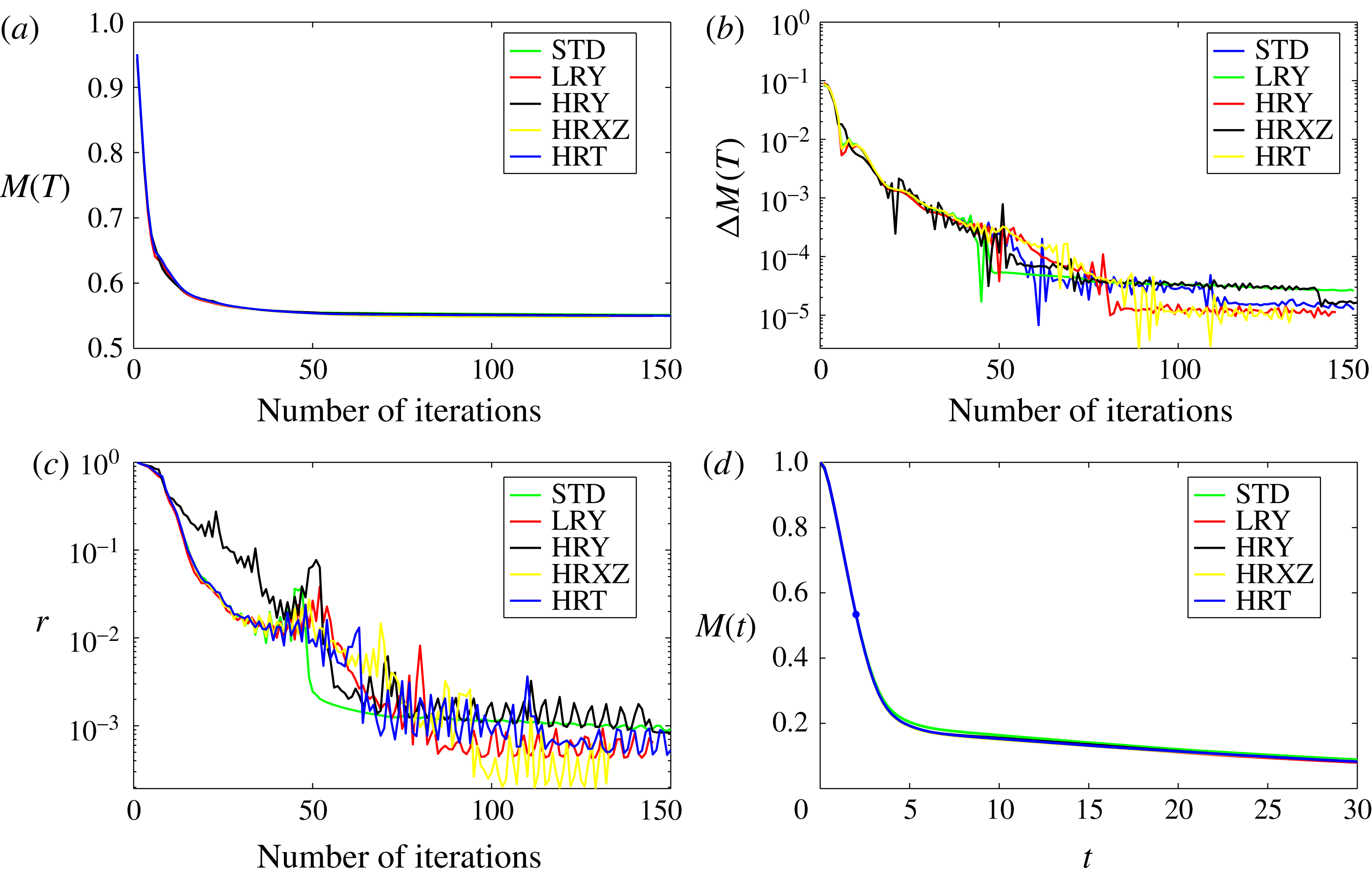
Following Rabin et al. (Reference Rabin, Caulfield and Kerswell2012) and Foures et al. (Reference Foures, Caulfield and Schmid2013), we consider the convergence of our minimisation scheme through monitoring the scaled residual
 $r$
defined as
 $$\begin{eqnarray}\displaystyle r=\frac{\Vert \unicode[STIX]{x1D735}_{\boldsymbol{u}_{0}}{\mathcal{L}}^{\bot }\Vert _{L^{2}}^{2}}{\Vert \unicode[STIX]{x1D735}_{\boldsymbol{u}_{0}}{\mathcal{L}}\Vert _{L^{2}}^{2}}. & & \displaystyle\end{eqnarray}$$
The expression
 $\unicode[STIX]{x1D735}_{\boldsymbol{u}_{0}}{\mathcal{L}}^{\bot }$
denotes the projection of the gradient
 $\unicode[STIX]{x1D735}_{\boldsymbol{u}_{0}}{\mathcal{L}}$
onto the hyperplane tangential to the energy hypersurface (2.23). We consider a sufficient criterion for adequate convergence to a local minimum to be
 $r\simeq O(10^{-3})$
.
3 Results
We solve the optimisation problem (2.26) using the DAL method as described in the previous section. We consider five different target times,
 $T=2,5,10,20,30$
, and two values of Reynolds number. Firstly, in order to generalise the analysis of Foures et al. (Reference Foures, Caulfield and Schmid2014) to three dimensions, we investigate flows with the same, moderate Reynolds number
 $Re=500$
. Secondly, we consider a larger value of
 $Re=3000$
. Although such pressure-driven channel flows are linearly stable to normal modes for
 $Re\leqslant Re_{c}\approx 5772.22$
(Orszag Reference Orszag1971), it has been observed that turbulence transition can occur in the form of turbulent spots at subcritical Reynolds numbers as low as
 $Re_{T}\approx 1300$
(Carlson, Widnall & Peeters Reference Carlson, Widnall and Peeters1982; Klingmann Reference Klingmann1992; Lemoult, Aider & Wesfreid Reference Lemoult, Aider and Wesfreid2012). Since we are allowing finite-amplitude initial perturbations, we believe that
 $Re=3000$
is a natural choice, as it is an integer multiple of the value used by Foures et al. (Reference Foures, Caulfield and Schmid2014), clearly in the range of
 $Re$
where subcritical transition is possible, and yet still significantly lower than the critical
 $Re_{c}$
for linear instability.
Following Foures et al. (Reference Foures, Caulfield and Schmid2014), we solve the problem (2.26) for three different specific optimisations: maximisation of the (in general finite-amplitude) time-integrated perturbation energy gain, minimisation of the mix-norm, and minimisation of the variance of the concentration over various time horizons. The DAL method identifies the (at least locally) optimal initial perturbations associated with each of these optimisations. Following the evolutions in time of these perturbations as solutions to (2.17)–(2.19) allows us to identify the key physical mechanisms that control such ‘optimal’ mixing. In order to capture the enhanced effect of advection on the homogenisation of the scalar concentration field over and above purely diffusive effects, we define the following quantitative measures:
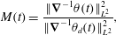 $$\begin{eqnarray}\displaystyle & \displaystyle M(t)=\frac{\Vert \unicode[STIX]{x1D735}^{-1}\unicode[STIX]{x1D703}(t)\Vert _{L^{2}}^{2}}{\Vert \unicode[STIX]{x1D735}^{-1}\unicode[STIX]{x1D703}_{d}(t)\Vert _{L^{2}}^{2}}, & \displaystyle\end{eqnarray}$$
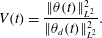 $$\begin{eqnarray}\displaystyle & \displaystyle V(t)=\frac{\Vert \unicode[STIX]{x1D703}(t)\Vert _{L^{2}}^{2}}{\Vert \unicode[STIX]{x1D703}_{d}(t)\Vert _{L^{2}}^{2}}. & \displaystyle\end{eqnarray}$$
Here,
 $\unicode[STIX]{x1D703}_{d}$
is the concentration of the scalar field evolving in the absence of any advection, i.e. it is a solution of
 $$\begin{eqnarray}\displaystyle \frac{\unicode[STIX]{x2202}\unicode[STIX]{x1D703}_{d}}{\unicode[STIX]{x2202}t}=Pe^{-1}\unicode[STIX]{x0394}\unicode[STIX]{x1D703}_{d},\quad \unicode[STIX]{x1D703}_{d}(\boldsymbol{x},0)=\unicode[STIX]{x1D703}_{0}(\boldsymbol{x}), & & \displaystyle\end{eqnarray}$$
with periodic boundary conditions in the horizontal directions and
 $$\begin{eqnarray}\displaystyle \frac{\unicode[STIX]{x2202}\unicode[STIX]{x1D703}_{d}}{\unicode[STIX]{x2202}y}=0\quad \text{on }\unicode[STIX]{x1D6E4}. & & \displaystyle\end{eqnarray}$$
Under the scaling (3.1) and (3.2), such purely diffusive processes correspond to time-independent quantities of
 $M(t)$
and
 $V(t)$
. Additionally, we introduce the appropriately scaled energy gain
 $$\begin{eqnarray}\displaystyle G(t)=\frac{1}{t}\frac{G_{E}(t)}{e_{0}|\unicode[STIX]{x1D6FA}|}, & & \displaystyle\end{eqnarray}$$
which quantifies the time-averaged kinetic energy growth of the perturbation. The two-dimensional version of the problem (2.26) was already investigated at
 $Re=500$
by Foures et al. (Reference Foures, Caulfield and Schmid2014), using an energy density of the initial perturbation
 $e_{0}=10^{-2}$
. For ease of comparison, we also use this value for both choices of Reynolds number, which proves to be large enough to allow the nonlinear effects to be significant.
3.1 Laminar regime:
$Re=500$

3.1.1 Time-averaged energy-growth maximisation
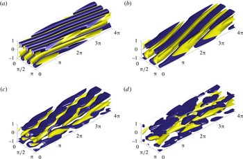
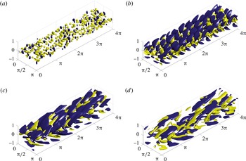
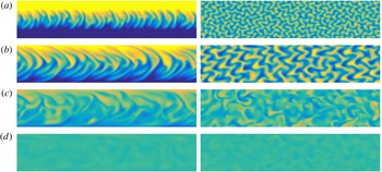
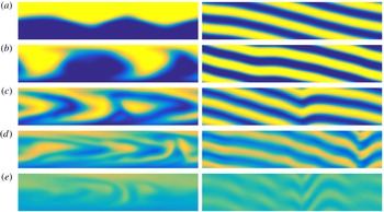
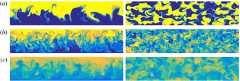
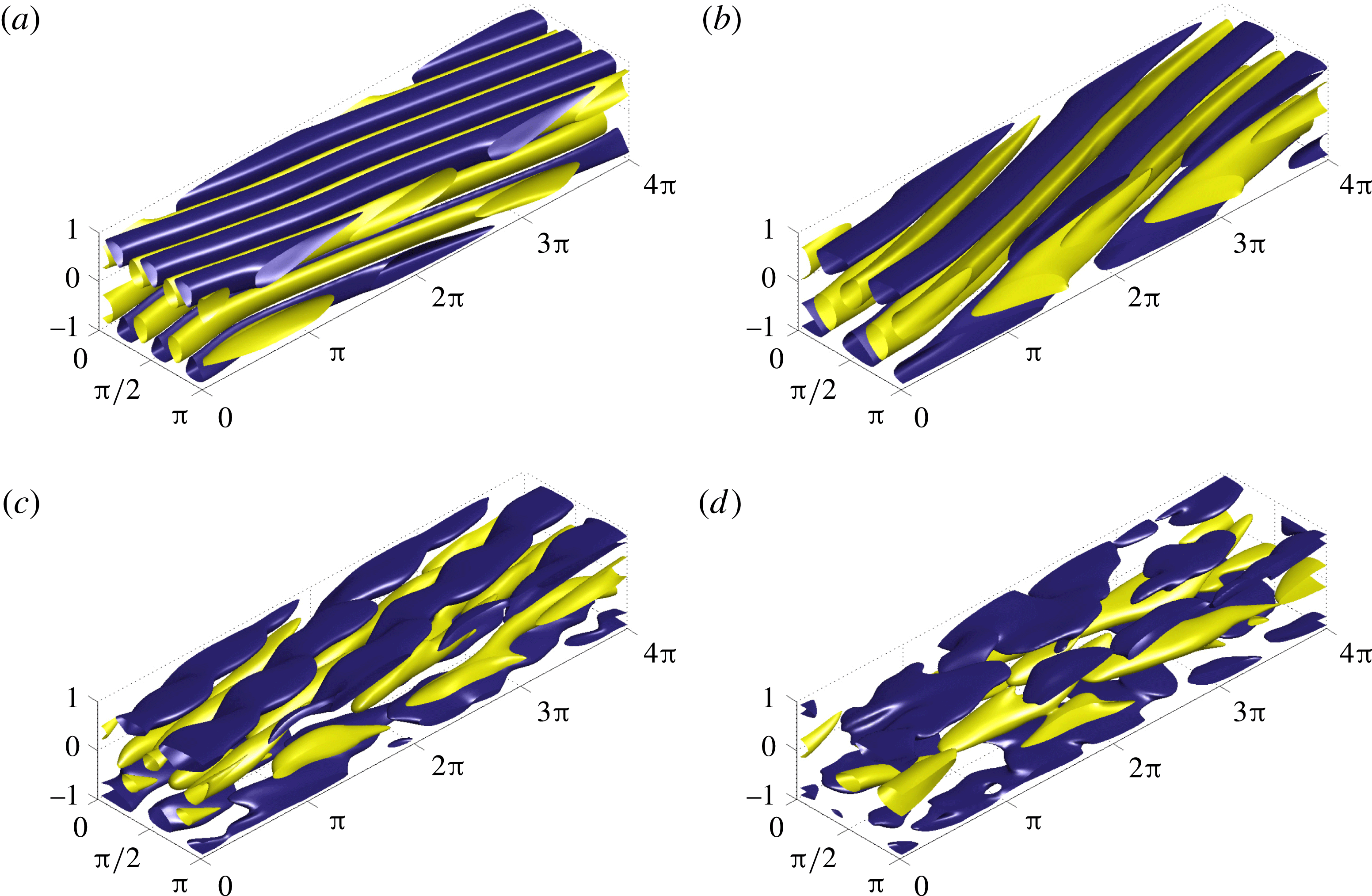
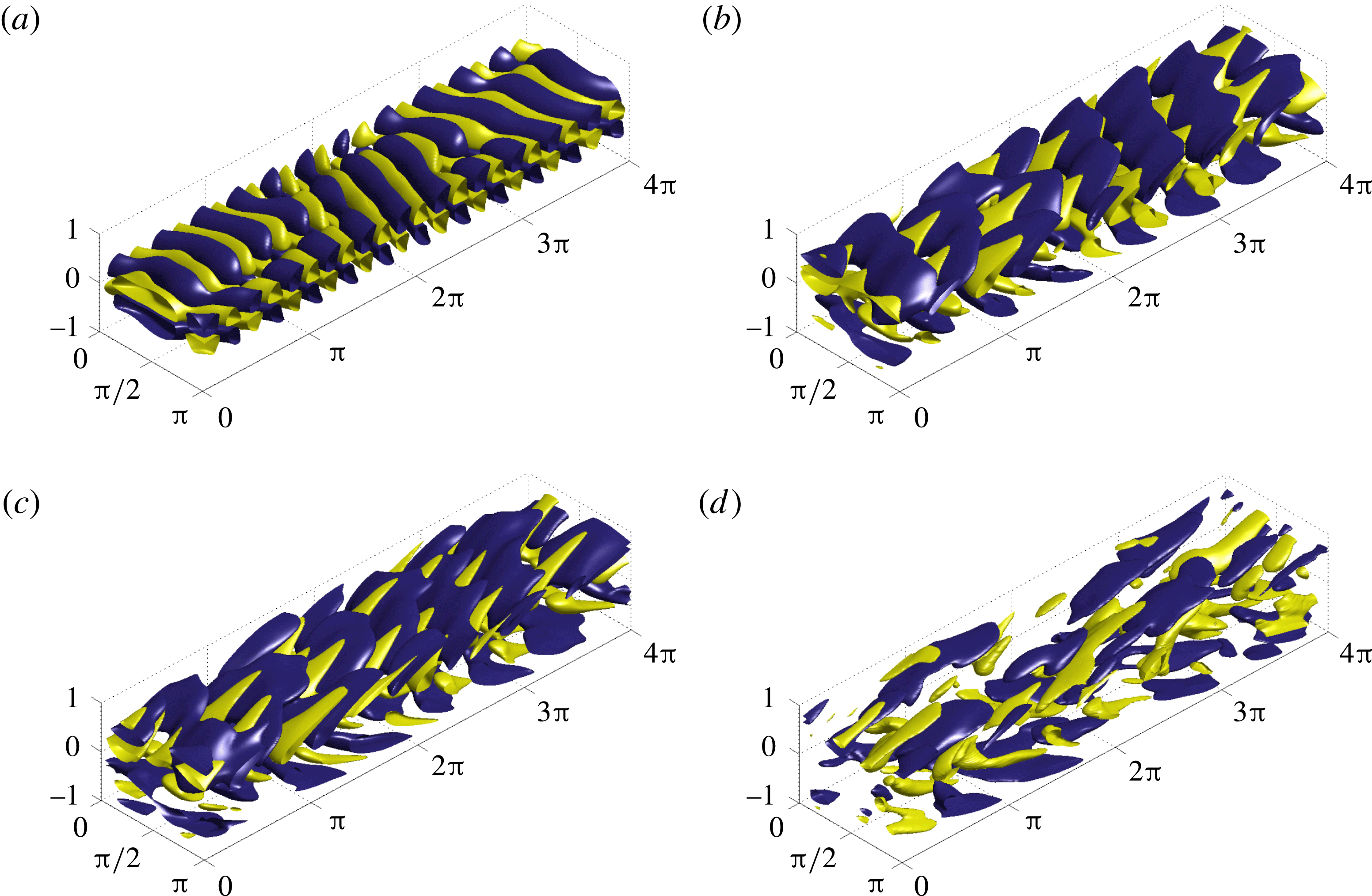
We first consider optimisation of time-averaged energy growth. In figure 3 we present the optimal initial flow perturbations for different time horizons. The panels show isosurfaces of the streamwise velocity component
 $u$
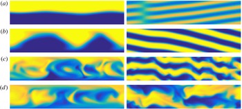
. In addition, in figure 4 we plot slices of the resulting concentration fields at the corresponding time horizons. On the left we plot the
 $z=\unicode[STIX]{x03C0}/2$
vertical plane, and on the right we plot the
 $y=0$
horizontal plane. It is apparent that, initially, the optimal perturbations take the form of vortices tilted against the direction of the mean shear. As time progresses, these vortices get rearranged and reoriented, resulting in transient and relatively rapid energy transfer from the base flow to the perturbation through the well-known process now known as the ‘Orr mechanism’ (Orr Reference Orr1907).
Optimal initial conditions for maximising the time average of energy growth for a flow with
 $Re=500$
over time horizons (a)
 $T=2$
, (b)
 $T=5$
, (c)
 $T=10$
and (d)
 $T=20$
. Isosurfaces of 40 % of the maximum (yellow) and minimum (blue) of the streamwise velocity component
 $u$
are shown.
Spatial distribution of the scalar concentration field at the terminal time horizon for a flow initialised by perturbations which maximise the time-average of energy growth for (a)
 $T=2$
, (b)
 $T=5$
, (c)
 $T=10$
and (d)
 $T=20$
on the vertical midplane at
 $z=\unicode[STIX]{x03C0}/2$
(left column) and the horizontal midplane
 $y=0$
(right column).
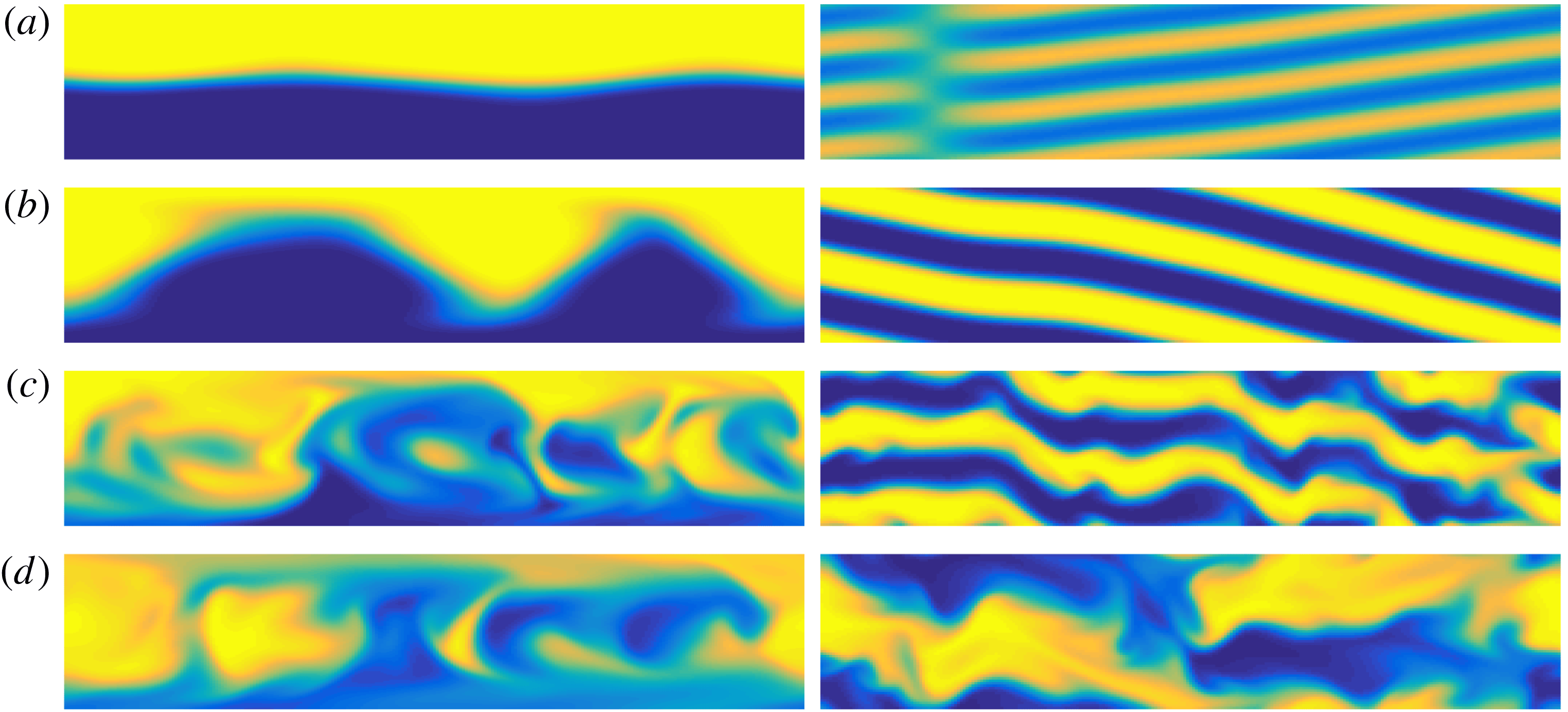
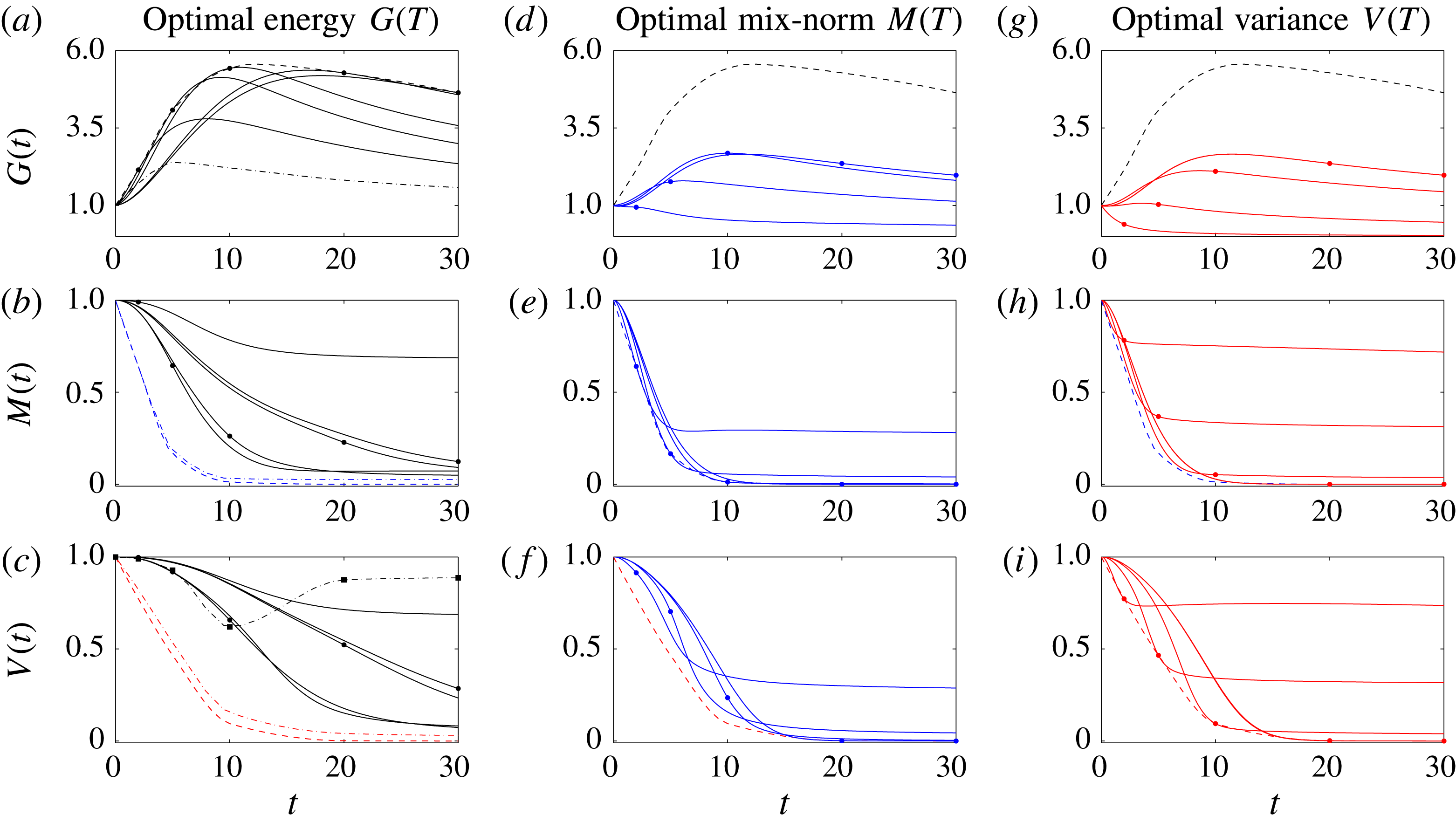
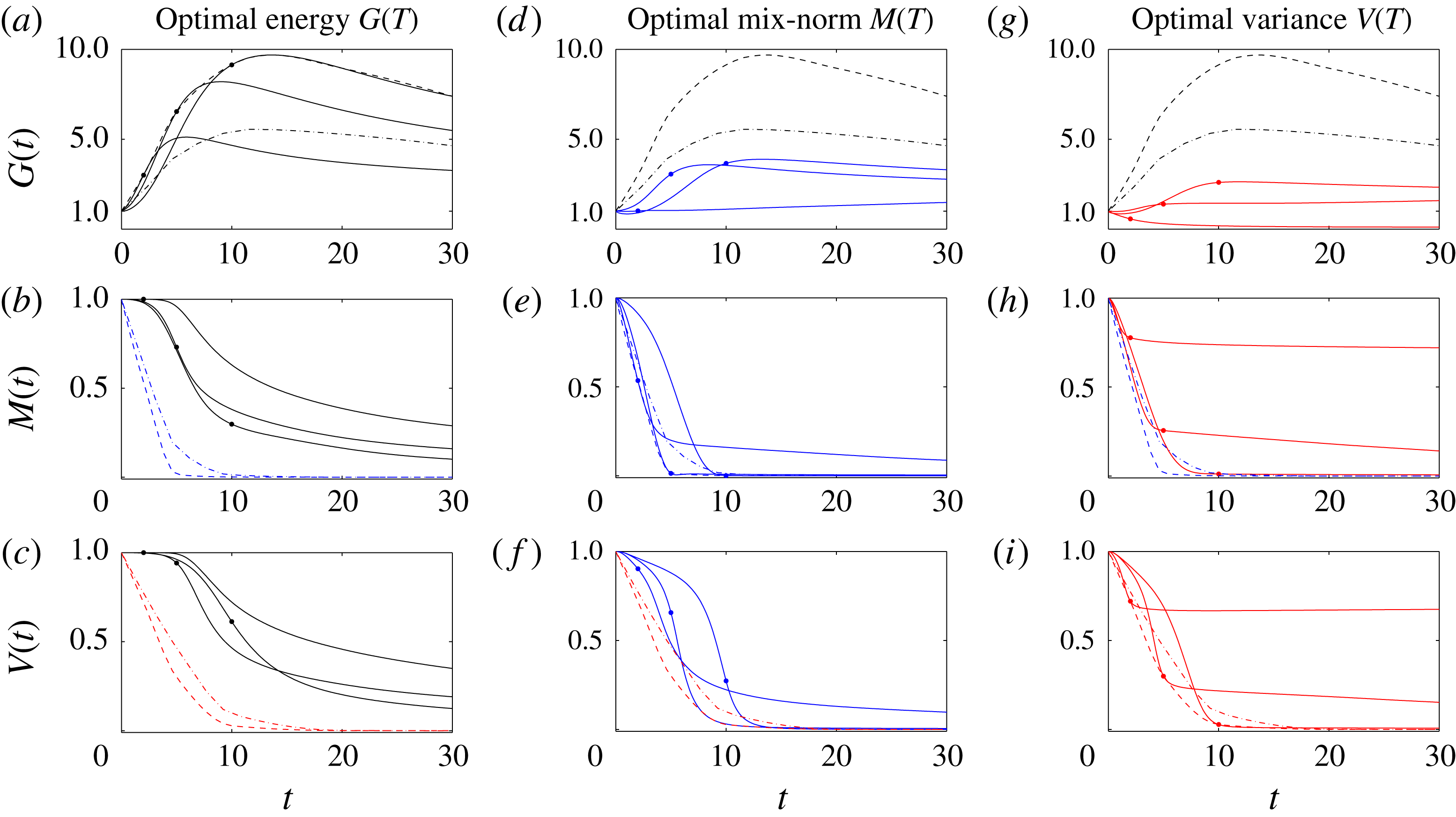
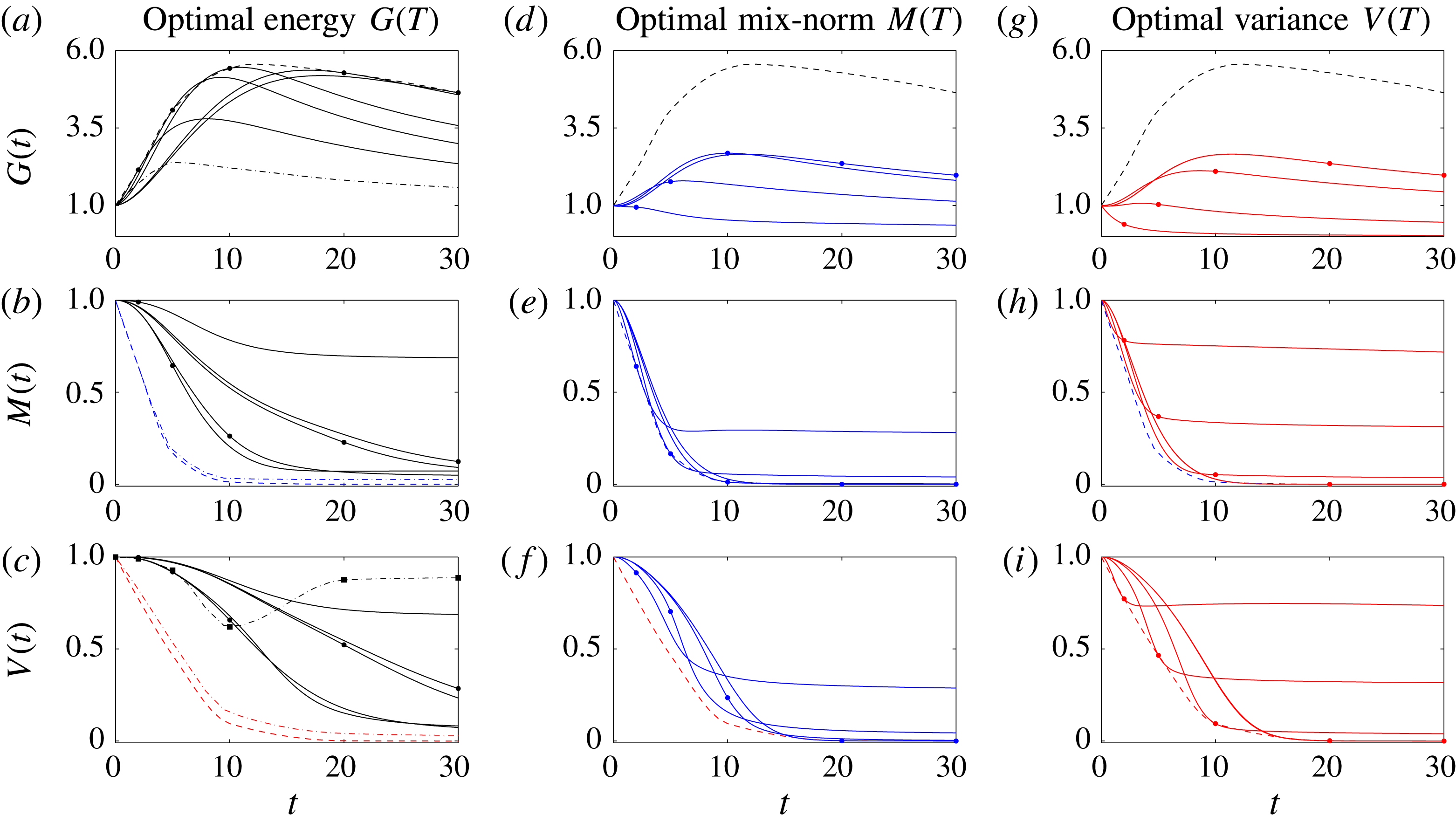
Figure 5(a) shows the time evolution of the time-averaged energy growth
 $G(T)$
(as defined in (3.5)) for the various time horizons. On each line the associated optimisation time horizon is marked with a black dot. The dashed line represents the optimal envelope
 $G_{opt}$
obtained by cubic interpolation of the optimal values
 $G(T)$
. (To capture the global maximum of
 $G_{opt}$
across all time horizons
 $T$
, an extra optimisation for time horizon
 $T=15$
is needed in order to capture the correct shape of the envelope.) For comparison, we also plot (with a dot-dashed line) the optimal envelope from the equivalent two-dimensional calculations in figure 5(a). Perhaps unsurprisingly, the energy growth in the three-dimensional flow is significantly larger than in the flow restricted to evolve purely in two dimensions. It is apparent from the structures of the initial perturbations shown in figure 3 that the perturbations have non-trivial spanwise structure, taking the form of obliquely aligned ‘streaks’. Such structures are also able to extract energy from the base flow via the ‘lift-up’ mechanism (see Landahl (Reference Landahl1980) and Brandt (Reference Brandt2014) for a detailed discussion), a mechanism which is only accessible to such inherently three-dimensional flows, and is also consistent with linear stability analyses (see Schmid & Henningson (Reference Schmid and Henningson2001) for more details).
Time evolution of the three studied measures for the three optimisation problems contained in (2.26) at
 $Re=500$
. For each of the initial perturbations, the rows show: (a,d,g) the time-averaged energy growth
 $G(t)$
; (b,e,h) the mix-norm
 $M(t)$
; and (c,f,i) the variance
 $V(t)$
of the concentration field. The perturbations associated with the different optimisation problems are shown in the columns: (a–c) maximisation of the time-averaged energy growth; (d–f) minimisation of the mix-norm; and (g–i) variance. The quantities
 $G(t)$
,
 $M(t)$
and
 $V(t)$
are defined in (3.5), (3.1) and (3.2), respectively. Thus, the time evolution of the optimal perturbations which actually optimise the specific quantities are shown in the panels located on the diagonal. Each panel contains five plots corresponding to the five chosen time horizons,
 $T=2,5,10,20,30$
. The associated time horizon for each plot is indicated by a dot. The optimal envelopes
 $G_{opt}^{L}(T)$
,
 $M_{opt}^{L}(T)$
and
 $V_{opt}^{L}(T)$
(plotted with dashed lines) are obtained via cubic interpolation of the optimal values at the time horizons, and the envelopes are plotted in all the panels of each row to allow better comparison between the various optimisation problems. In (a) to (c) the dot-dashed lines represent the optimal envelopes
 $G_{opt}^{2D}(T)$
,
 $M_{opt}^{2D}(T)$
and
 $V_{opt}^{2D}(T)$
obtained by Foures et al. (Reference Foures, Caulfield and Schmid2014) from flows restricted to evolve in two dimensions. The squares in (c) indicate the values of the scaled variance produced by energy-growth-maximising perturbations in two dimensions at the specific target times as reported by Foures et al. (Reference Foures, Caulfield and Schmid2014). The black dot-dashed line in (c) corresponds to the cubic interpolation of these data points.
Furthermore, Foures et al. (Reference Foures, Caulfield and Schmid2014) demonstrated that, when the flow was restricted to be two-dimensional, initial perturbations which optimise the energy amplification proved not to be effective mixers. Particularly, for larger target times (e.g.
 $T=20,30$
) enhancements in mixing associated with advection above pure diffusion was very weak, when measured in terms of reduction in either the variance or the mix-norm. In figure 5(c), we plot the time evolution of the variance of the scalar concentration field associated with the flow initialised by the perturbations which maximise time-averaged energy growth. The circles on each of the curves once again mark the terminal time of the interval over which the optimisation takes place. The black squares show the value of concentration variance at the terminal time of the optimisation interval for the equivalent inherently two-dimensional flows initialised by perturbations which optimise time-averaged energy growth. The three-dimensional perturbations associated with energy-growth optimisation lead to more (though still not thorough) mixing than the equivalent two-dimensional perturbations.
Indeed, there appears to be three different characteristic behaviours. First, for the shortest time interval of optimisation
 $T=2$
, little reduction in variance ensues. The highly organised perturbations plotted in figure 3(a) are localised near the walls, and so their growth does not induce significant filamentation, and hence little mixing occurs.
Conversely, for the two longer time horizons
 $T=20$
and
 $T=30$
, the initial perturbation is really rather unstructured. (This structure is suggestive of the method only having identified a local maximum, as it is plausible that another similarly unstructured perturbation would have very similar, and perhaps even higher, time-averaged perturbation growth.) As is apparent in figure 4, these unstructured perturbations remain unstructured throughout flow evolution, leaving patchiness (and thus non-trivial variance) in the concentration field throughout its evolution. Finally, the intermediate time horizons (of
 $T=5$
and
 $T=10$
) are interestingly better at reducing variance by
 $t=30$
, as the more structured initial perturbation, combined crucially with an earlier peak in perturbation energy, appears to be able to exploit filamentation and hence transport at intermediate times to ensure a superior performance in mixing. Of course, this does not violate the optimisation procedure, as there is no a priori reason why these perturbations should lead to ‘good’ variance reduction, as already noted by Foures et al. (Reference Foures, Caulfield and Schmid2014) for two-dimensional flow.
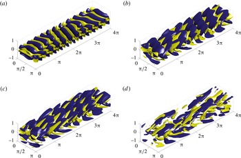
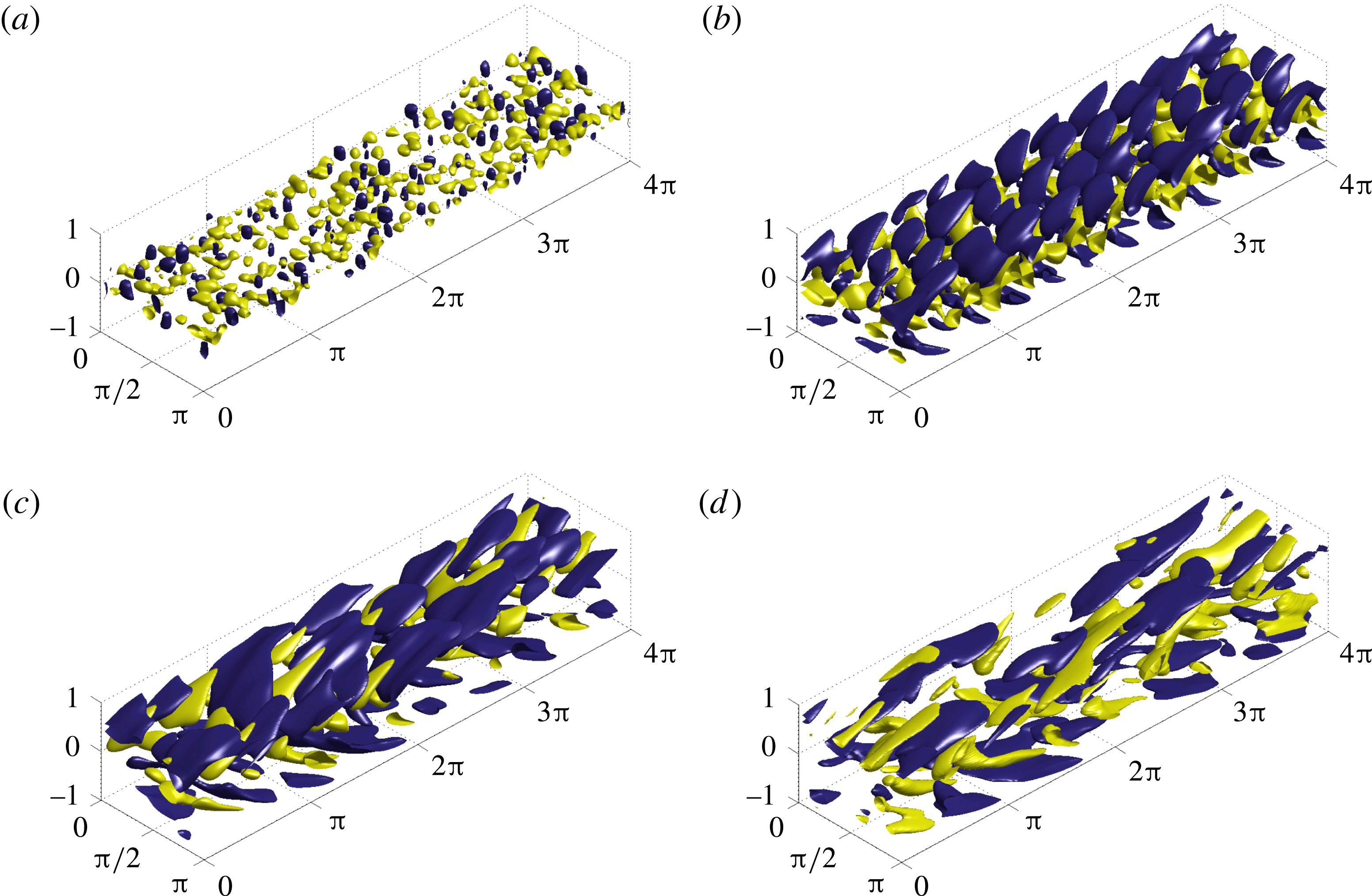
Optimal initial conditions for minimising the variance for a flow with
 $Re=500$
over time horizons: (a)
 $T=2$
, (b)
 $T=5$
, (c)
 $T=10$
and (d)
 $T=20$
. Isosurfaces of 40 % of the maximum (yellow) and minimum (blue) of the streamwise velocity component
 $u$
are shown.
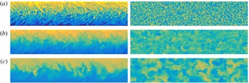
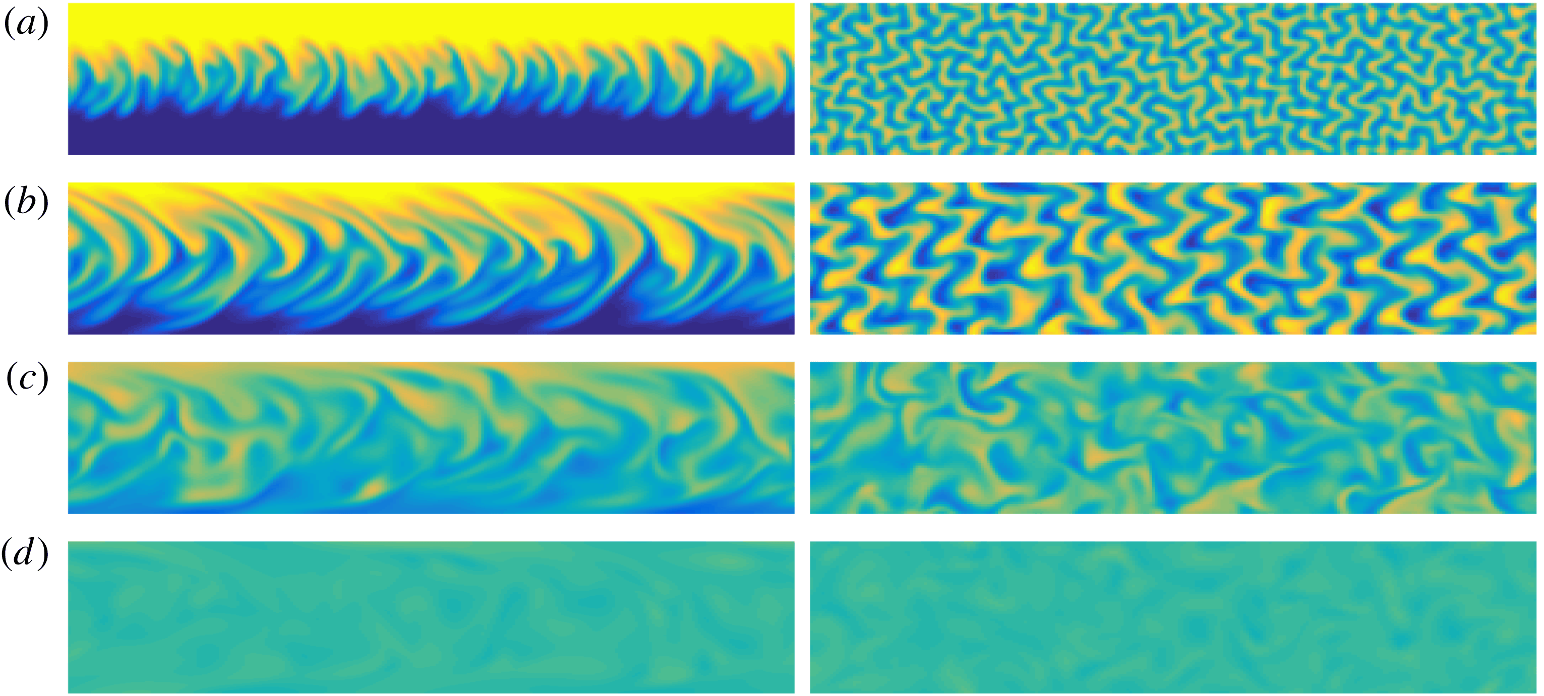
Spatial distribution of the scalar concentration field at the terminal time horizon for a flow initialised by perturbations which minimise the variance for (a)
 $T=2$
, (b)
 $T=5$
, (c)
 $T=10$
and (d)
 $T=20$
on the vertical midplane at
 $z=\unicode[STIX]{x03C0}/2$
(left column) and the horizontal midplane
 $y=0$
(right column).
3.1.2 Variance minimisation
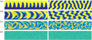
To explore further which initial perturbations are actually optimal in three-dimensional flow at these Reynolds numbers, we consider initial perturbations that minimise the variance of the passive scalar at the selected time horizons. We plot these perturbations in figure 6, while we plot the resulting distribution of the passive scalar at the time horizon in figure 7. In contrast to the perturbations associated with maximum time-averaged energy growth, for short time horizons the variance-optimal perturbations take the form of small-scale vortices localised near the interface between the two different concentrations. These vortices perturb the interface and the passive scalar is transported through small-scale ‘wrinkles’. In particular, the top-view plots reveal that, for the shorter time horizons, the wrinkles are densely woven into each other such that the contact interface between the two layers is highly extended. Consequently, large regions of strong concentration gradients are created, which allows diffusion to occur in a central mixing layer. The scale of the initial vortices increases such that the wrinkles penetrate further across the channel as the target time is increased, as is apparent in figure 6. Figure 5(i) shows the optimal variance evolution in time
 $V(t)$
for the selected time horizons. We see that, after reaching the chosen time horizon, the variance reaches a plateau and so mixing proceeds at a rate corresponding to the advection-free system (3.3).
To understand how the ultimate amount of mixing triggered by these various perturbations varies with time horizon, we plot with a dashed line in figure 5(i) the optimal envelope
 $V_{opt}^{L}$
obtained by cubic interpolation of the variances at the target times. We also plot the time evolution of the variances for the different individual target time horizons (marked with a dot on each curve). It is clear that the optimisations over short time horizons (i.e. with
 $T=2$
and
 $T=5$
) do not fully mix the passive scalar, and it is only the longer time horizons which approach close to full mixing. Furthermore, figure 5(c) shows the two-dimensional counterpart of
 $V_{opt}^{L}$
(represented by dot-dashed line). We see that the mixing behaviour of the variance-optimal strategy does not change dramatically when moving from two-dimensional flow to three-dimensional flows at this
 $Re$
. For instance, for the target time
 $T=30$
, the three-dimensional optimal perturbation yields mixing that is only 3 % more effective (in the sense of reduction in variance) than the optimal perturbation in a flow restricted to two dimensions. Following the analysis of Foures et al. (Reference Foures, Caulfield and Schmid2014), we also consider the energy gain of the variance-optimising perturbations in figure 5(g). Once again we find that these perturbations undergo a much smaller energy gain than the energy-gain-optimising perturbations, reinforcing the conclusion of Foures et al. (Reference Foures, Caulfield and Schmid2014) that energy gain can actually be counter-productive to extensive mixing, at least at these Reynolds numbers.
3.1.3 Mix-norm minimisation
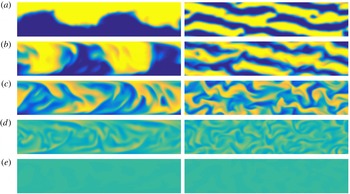
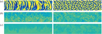
Finally, in figure 8, we present the initial perturbations that minimise the mix-norm of the passive scalar at the selected target times, while in figure 9 we show the resulting concentration fields. Although the mix-norm-optimal perturbations have some points of similarity with the variance-optimal perturbations (i.e. as the target time increases, the characteristic scales become larger, and the perturbations become more streamwise-aligned), there are still some substantial differences, particularly at early times. Perhaps unsurprisingly, since the mix-norm strongly penalises small scales, the mix-norm-optimal perturbations consist of coherent structures that disturb the interface of the two layers, forming quasi-wall-normal bands in which the passive scalar is periodically transported into the regions of opposite concentration in a way that proves effective in ultimately mixing the concentration field. Indeed, as is clear from figure 5(f,g), for all except the shortest target time
 $T=2$
, all the mix-norm-optimal perturbations lead to excellent mixing, in the sense that the variance at
 $T=30$
is small.
Optimal initial conditions for minimising the variance for a flow with
 $Re=500$
over time horizons (a)
 $T=2$
, (b)
 $T=5$
, (c)
 $T=10$
and (d)
 $T=20$
. Isosurfaces of 40 % of the maximum (yellow) and minimum (blue) of the streamwise velocity component
 $u$
are shown.
Spatial distribution of the scalar concentration field at the terminal time horizon for a flow initialised by perturbations which minimise the mix-norm for (a)
 $T=2$
, (b)
 $T=5$
, (c)
 $T=10$
and (d)
 $T=20$
on the vertical midplane at
 $z=\unicode[STIX]{x03C0}/2$
(left column) and the horizontal midplane
 $y=0$
(right column).
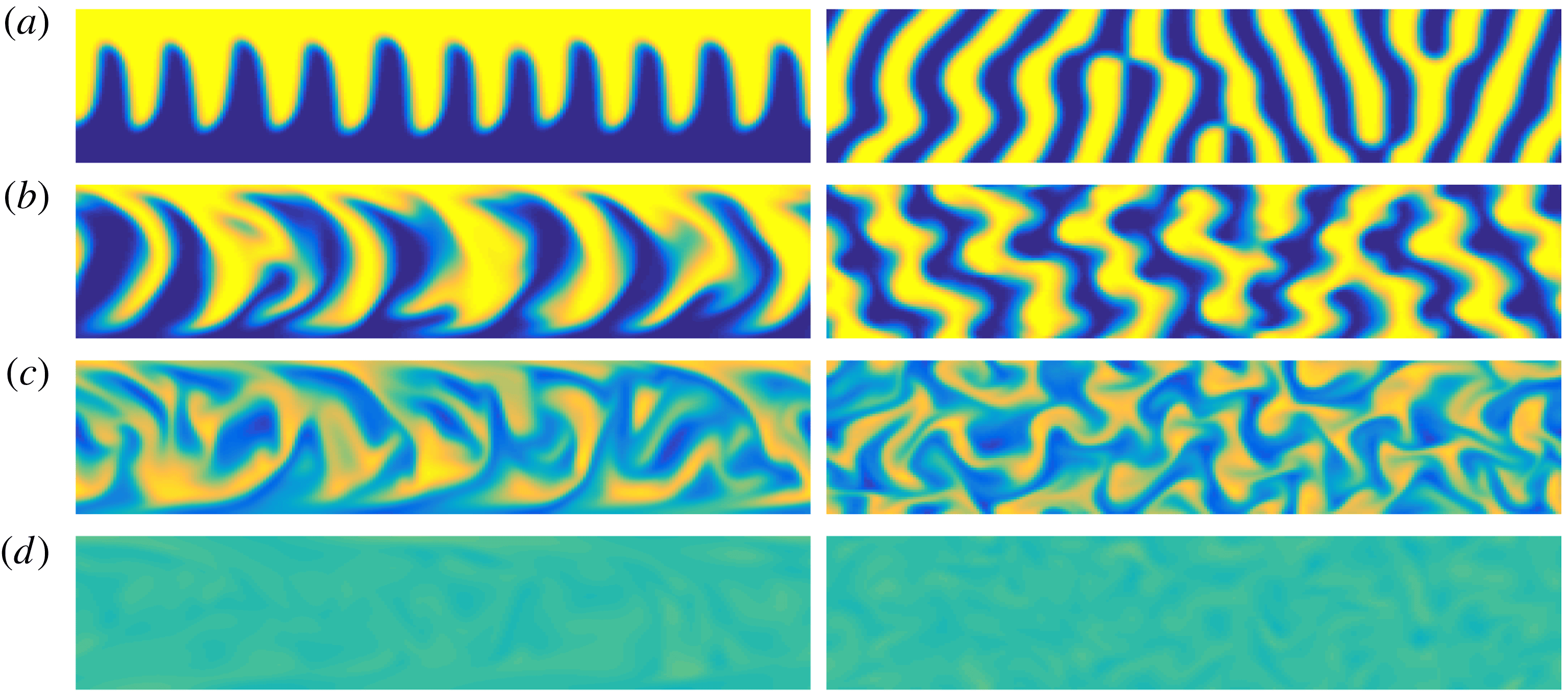
This suggests a particular utility of the mix-norm optimisation problem. Shorter target times are computationally cheaper, and, as is apparent from consideration of the isosurface structures, the optimal perturbations identified over longer target times have some disorder, suggesting, as already noted, that they might correspond to a specific local maximum from a class of similar initial perturbations. However, when minimising variance, the short-time-horizon optimal perturbations do not approach closely to the solution trajectory associated with thorough mixing identified by the long-time-horizon optimal perturbations, possibly due to the (already discussed) issue that the rate of decay of the variance is constrained by the small value of
 $1/Pe$
.
There is no such constraint on the mix-norm optimisation problem, and indeed the time evolution of the optimal perturbation which minimises the mix-norm at
 $T=5$
effectively traces close to the time evolution of the ‘true’ optimal perturbation to minimise variance for
 $T=30$
. Therefore, algorithmically, it seems wise to use mix-norm optimisations over short target times as proxies for substantially more computationally demanding variance optimisations over longer target times, as mix-norm optimisation is far less sensitive to the choice of target time than the strategy that focuses on variance.
3.2 Time evolution of the optimal perturbations
Before considering the effect of variations in
 $Re$
on this observed usefulness of the mix-norm optimisation problem, we consider the evolution of the various optimal perturbations in more detail. Firstly, for energy-growth optimisation, we choose the time horizon
 $T=5$
to allow comparison with the two-dimensional analyses presented in Foures et al. (Reference Foures, Caulfield and Schmid2014). Figure 10 displays the evolution of the concentration variance under the action of the optimal perturbation at several times
 $t\in [0,30]$
. Initially, at
 $t=0$
the perturbation flow field (shown in figure 3
b) creates vortices tilted against the mean shear direction. The rearrangement and reorientation of the vortices generate transient energy growth that the perturbation experiences before it starts to decay exponentially, essentially exploiting the Orr mechanism.
The vortices distort the interface into a wave and effectively give rise to stripe-like regions in which the passive scalar is transported up and down in alternate fashion (figure 10 a). Consequently, the interface is extended, which allows the diffusion over a larger surface area. It is worth noting that at this stage the flow field is almost invariant with respect to a shift in the third spanwise direction. Spectral analysis shows that the observed structure is effectively a superposition of two waves which have the same spanwise frequency but different streamwise frequency. Therefore, these waves travel at different phase velocity along the channel and in particular, as time progresses, the wave crests and wave troughs are pushed towards the channel walls – to the regions of strong shear, which enhances the mixing, as the stripes are distorted into angled chevrons. Moreover, stretching the interface across the channel allows the constant shear of the base flow to contribute to mixing of the passive scalar (figure 10 b).
In the study of purely two-dimensional flow, Foures et al. (Reference Foures, Caulfield and Schmid2014) state that the advection eventually starts to act against the tendency of the flow to mix, and indeed eventually resegregates the scalar layers. Interestingly, this does not occur in the inherently three-dimensional flow because the three-dimensional vorticity dynamics allows for an extra transport of the passive scalar in the spanwise direction, as can be seen in figure 10(c,d). The resulting shear enhancement intensifies the mixing and eventually leads to a comparatively more homogeneous distribution of the passive scalar field, as shown in figure 10(e).
Time evolution of the scalar field distribution produced by the energy-growth optimal perturbation (with time horizon
 $T=5$
) at (a)
 $t=2$
, (b)
 $t=7$
, (c)
 $t=12$
, (d)
 $t=18$
and (e)
 $t=30$
, on the vertical midplane at
 $z=\unicode[STIX]{x03C0}/2$
(left column) and the horizontal midplane
 $y=0$
(right column).
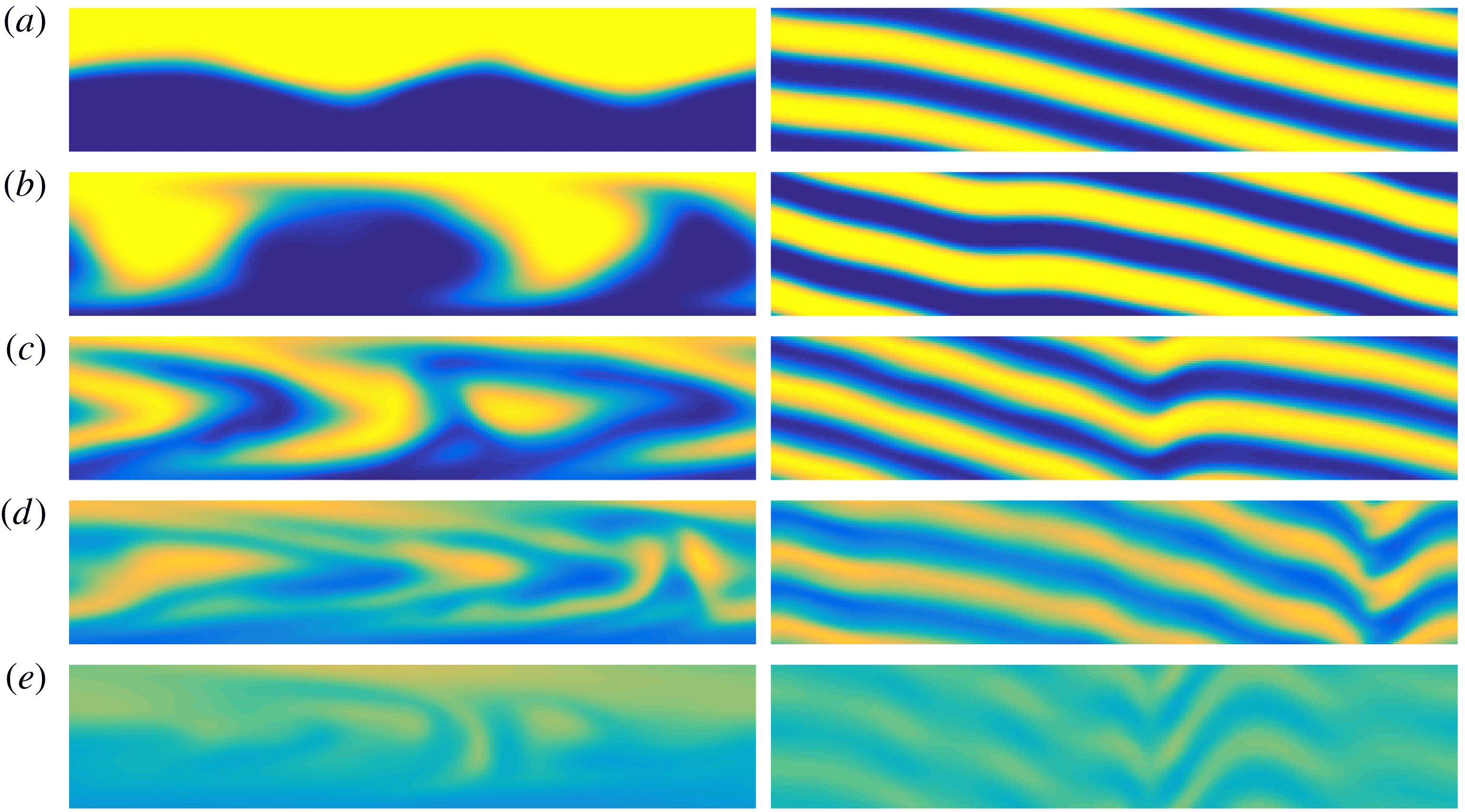
To quantify our observations, we study the production term in (2.5), i.e. the term through which the perturbation flow field acts on the concentration gradient and influences the rate of mixing. Let us define
 $$\begin{eqnarray}\displaystyle & \displaystyle P_{\bar{u}}(y,t)=\frac{1}{4\unicode[STIX]{x03C0}^{2}}\int _{0}^{4\unicode[STIX]{x03C0}}\!\!\int _{0}^{\unicode[STIX]{x03C0}}\unicode[STIX]{x1D735}\unicode[STIX]{x1D703}\boldsymbol{\cdot }\unicode[STIX]{x1D735}\bar{\boldsymbol{u}}\boldsymbol{\cdot }\unicode[STIX]{x1D735}\unicode[STIX]{x1D703}\,\text{d}z\,\text{d}x=-\frac{y}{2\unicode[STIX]{x03C0}^{2}}\int _{0}^{4\unicode[STIX]{x03C0}}\!\!\int _{0}^{\unicode[STIX]{x03C0}}\unicode[STIX]{x2202}_{x}\unicode[STIX]{x1D703}\unicode[STIX]{x2202}_{y}\unicode[STIX]{x1D703}\,\text{d}z\,\text{d}x, & \displaystyle\end{eqnarray}$$
 $$\begin{eqnarray}\displaystyle & \displaystyle P_{u}(y,t)=\frac{1}{4\unicode[STIX]{x03C0}^{2}}\int _{0}^{4\unicode[STIX]{x03C0}}\!\!\int _{0}^{\unicode[STIX]{x03C0}}\unicode[STIX]{x1D735}\unicode[STIX]{x1D703}\boldsymbol{\cdot }\unicode[STIX]{x1D735}\boldsymbol{u}\boldsymbol{\cdot }\unicode[STIX]{x1D735}\unicode[STIX]{x1D703}\,\text{d}z\,\text{d}x, & \displaystyle\end{eqnarray}$$
 $$\begin{eqnarray}\displaystyle & \displaystyle P_{d}(y,t)=\frac{1}{4\unicode[STIX]{x03C0}^{2}}\int _{0}^{4\unicode[STIX]{x03C0}}\!\!\int _{0}^{\unicode[STIX]{x03C0}}|\unicode[STIX]{x1D735}\unicode[STIX]{x1D703}|^{2}\,\text{d}z\,\text{d}x. & \displaystyle\end{eqnarray}$$
The quantities
 $P_{\bar{u}}(y,t)$
and
 $P_{u}(y,t)$
represent the evolution of the horizontally averaged reduction of the concentration gradient due to the actions of the base flow
 $\bar{u}$
and the perturbation (not necessarily ‘small’) flow
 $u$
, respectively, while
 $P_{d}(y,t)$
denotes the evolution of the horizontally averaged concentration gradient. Furthermore, we split
 $P_{u}$
into two terms to distinguish the action in the
 $x$
–
 $y$
plane and the effects inherently linked to the three-dimensional nature of the problem, defining
 $$\begin{eqnarray}\displaystyle P_{2D}(y,t)=\frac{1}{4\unicode[STIX]{x03C0}^{2}}\int _{0}^{4\unicode[STIX]{x03C0}}\!\!\int _{0}^{\unicode[STIX]{x03C0}}\mathop{\sum }_{i,j=1}^{2}\unicode[STIX]{x2202}_{i}\unicode[STIX]{x1D703}\unicode[STIX]{x2202}_{i}u_{j}\unicode[STIX]{x2202}_{j}\unicode[STIX]{x1D703}\,\text{d}z\,\text{d}x,\quad P_{3D}=P_{u}-P_{2D}. & & \displaystyle\end{eqnarray}$$
Figure 11 shows the time evolution of the various production terms defined in (3.6)–(3.9). From figure 11(b) showing
 $P_{u}(y,t)$
, it is apparent that the perturbation velocity field initially accelerates mixing on the interface between the two layers of the passive scalar, while later for
 $t\gtrsim 5$
, it exploits strong shear in the wall regions. The plot of
 $P_{\bar{u}}(y,t)$
in figure 11(a) confirms that the vertical transport of the passive scalar is additionally accompanied by a shear due to the base flow. The final stirring action takes place at an intermediate distance between the walls and the centre of the channel. In figures 11(c) and 11(d) we plot
 $P_{2D}$
and
 $P_{3D}$
, respectively. We see that the shear-enhanced mixing in the regions close to the walls is linked purely with the action in the
 $x{-}y$
plane, while the later stirring is inherently based on the shear associated with the (third spanwise)
 $z$
-direction, thus differentiating the three-dimensional dynamics from the two-dimensional dynamics.
Time and wall-normal variation of the various production terms (as defined in (3.6)–(3.9)) for the optimal flow for energy growth over a time horizon of
 $T=5$
: (a) the base flow term
 $P_{\bar{u}}$
; (b) the (total) perturbation term
 $P_{u}$
; (c) the perturbation term in the
 $x$
–
 $y$
plane
 $P_{2D}$
; and (d) the three-dimensional deviation term
 $P_{3D}$
.
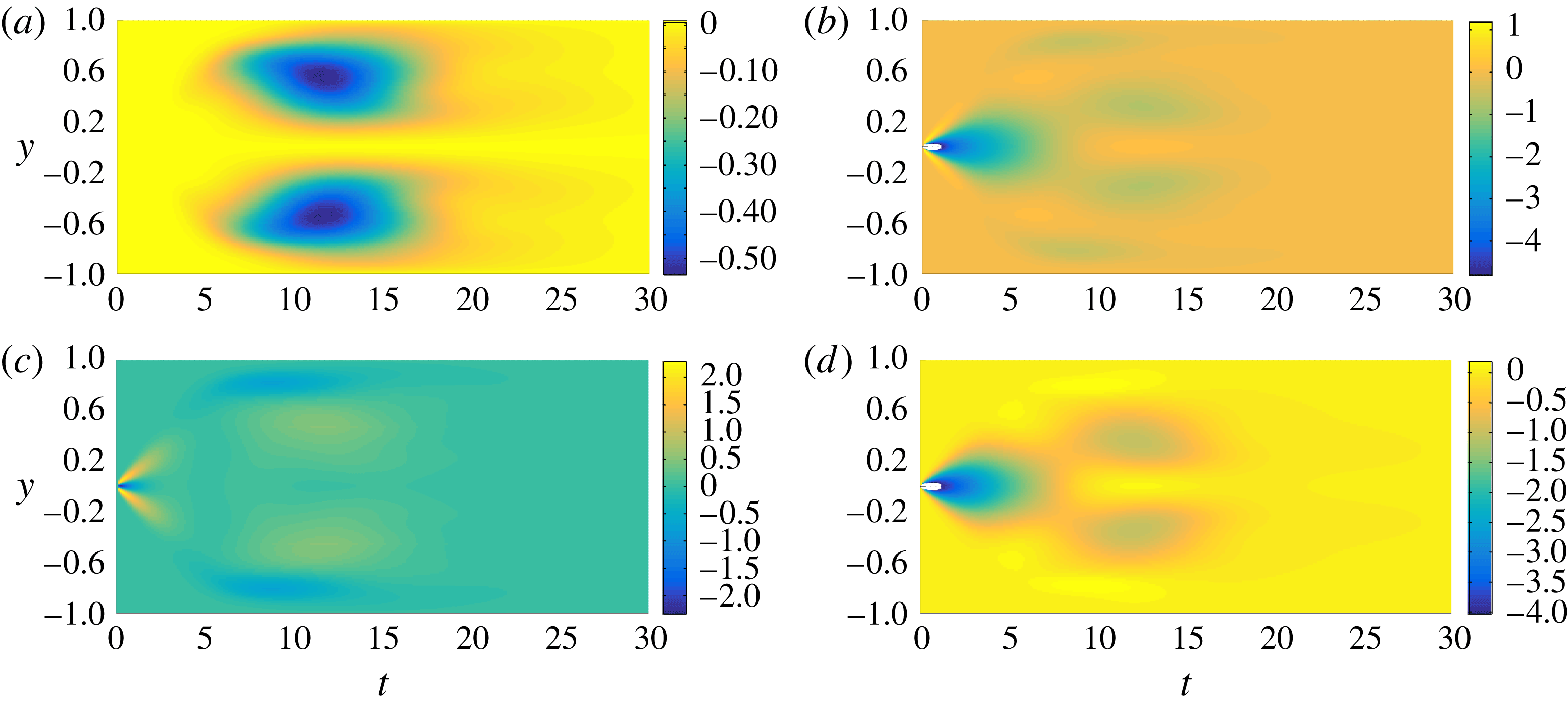
Time evolution of the scalar field distribution produced by the variance-optimal perturbation (with time horizon
 $T=30$
) at (a)
 $t=2$
, (b)
 $t=6$
, (c)
 $t=10$
, (d)
 $t=15$
and (e)
 $t=30$
, on the vertical midplane at
 $z=\unicode[STIX]{x03C0}/2$
(left column) and the horizontal midplane
 $y=0$
(right column).
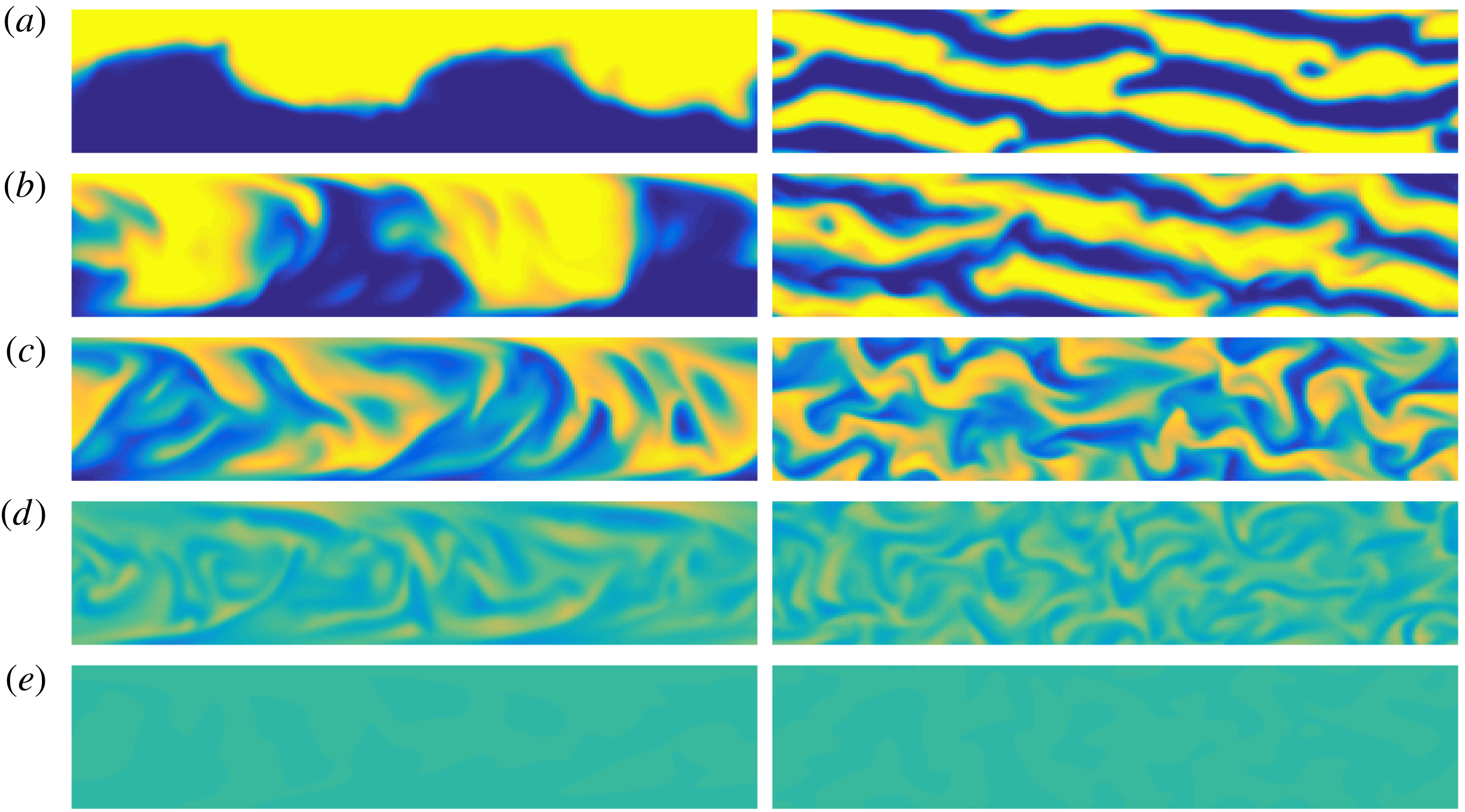
Naturally, a similar analysis can be applied to the variance-optimal perturbation. Here, once again, for the sake of comparison with the previously published two-dimensional analysis, we consider the flow as it evolves with an optimisation time horizon
 $T=30$
. In figure 12 we plot snapshots of the scalar field concentration at five indicative times, while in figure 13, similarly to figure 11, we plot the spatio-temporal variation of the production terms defined in (3.6)–(3.9).
Figures 12 and 13 show that the mixing is also driven by the same mechanisms which occur in the evolution of the energy-optimal perturbation. However, for this flow they are organised in such a way that the mixing impact at the chosen target time is maximal. Fundamentally, the three-dimensional mixing process as a whole passes through the three stages described for two-dimensional flow by Foures et al. (Reference Foures, Caulfield and Schmid2014), i.e. transport, then dispersion, then relaxation.
Firstly, the initial two-layer distribution of the passive scalar is perturbed so that large amounts of the scalar field are ‘transported’ into the region of opposite concentration. This upwards and downwards transport organises the concentration into (vertical) ‘stripe’ regions. This has two effects. Firstly, the interface where the concentration gradients are large is extended, which leads to an initial drop in the concentration variance. Secondly, once the interface comes close to the channel walls at
 $t\sim 3.5$
, the mixing is enhanced through ‘dispersion’ by the constant shear due to the base flow closely followed by the shear due to the perturbation field in the boundary region. Moreover, due to the inherently three-dimensional nature of the flow, extra spanwise transport occurs, with the stripe-like regions being effectively distorted such that the associated inherently spanwise
 $z$
-dependent shear further supports mixing. As is apparent from figure 13, the maximal contributions to mixing caused by these three shear production terms are comparable, and so we think it is appropriate to consider them of comparable importance. Finally, as time progresses, the production terms become so small such that by
 $t\sim 18$
neither the perturbation field nor the base flow are significantly affecting the distribution of the passive scalar. This is the final ‘relaxation’ stage of the mixing process when all inhomogeneities are smeared out by molecular diffusion. It is important to appreciate that, even though the time horizon for the optimisation is changed between the two cases shown in figures 10, 11 (for energy-growth maximisation with
 $T=5$
) and figures 12, 13 (for variance minimisation with
 $T=30$
), the optimal mixing process remains conceptually the same: it still comprises the three aforementioned stages – transport, dispersion and relaxation – with the dispersion stage being composed of the three contributing mechanisms of similar strength.
Time and wall-normal variation of the various production terms (as defined in (3.6)–(3.9)) for the variance-optimal flow over a time horizon of
 $T=30$
for a flow with
 $Re=500$
: (a) the base flow term
 $P_{\bar{u}}$
; (b) the (total) perturbation term
 $P_{u}$
; (c) the perturbation term in the
 $x{-}y$
plane
 $P_{2D}$
; and (d) the three-dimensional deviation term
 $P_{3D}$
.
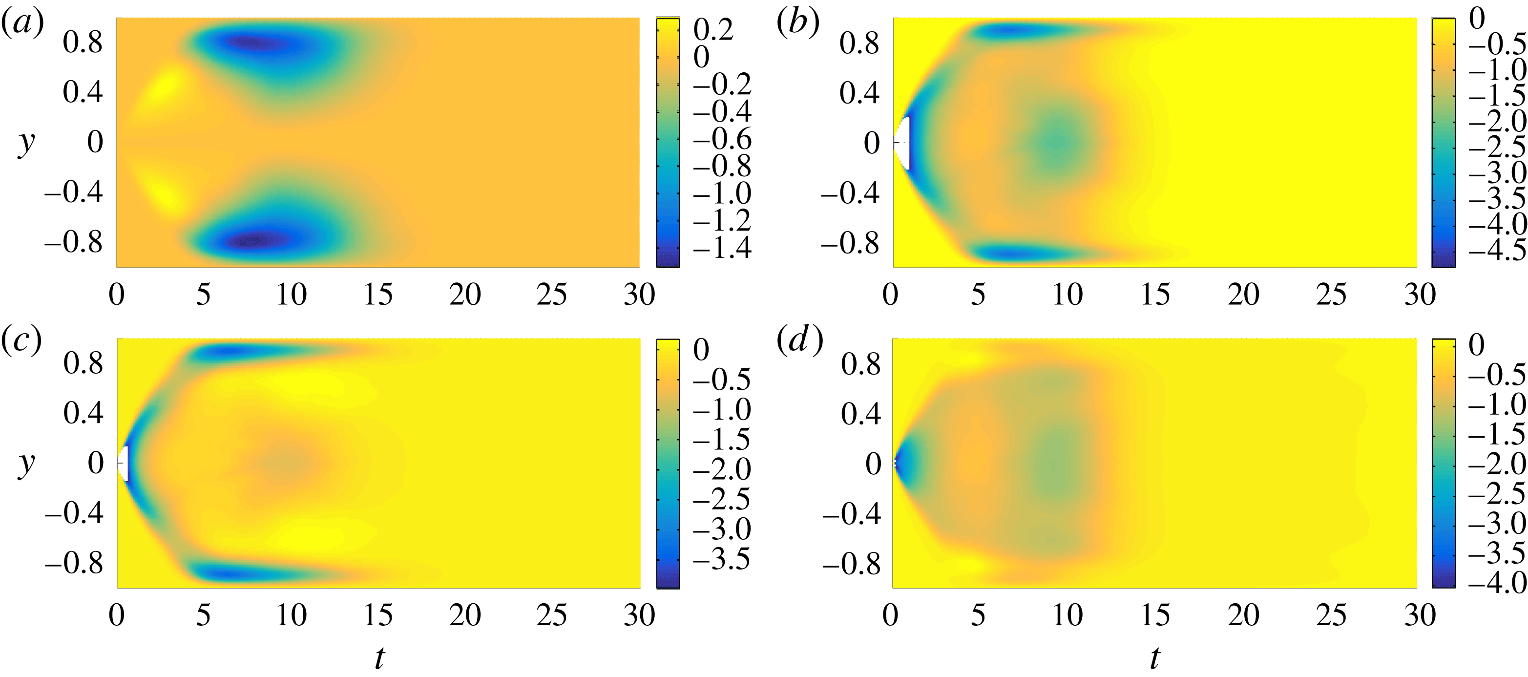
3.3 Transitional mixing:
$Re=3000$

In the previous section we studied the properties of the three different optimisation problems in flows with
 $Re=500$
. In this section we wish to explore the effect of variation of Reynolds number, in particular when the Reynolds number is sufficiently large for the flow to behave in a qualitatively different fashion. We choose
 $Re=3000$
, as this is a sufficiently large value for the flow to undergo turbulence transition. We carry out a similar analysis of the problem (2.26) as in the previous sections. We solve the same three optimisation problems, corresponding to maximisation of the time-integrated energy growth, mix-norm minimisation and variance minimisation. As simulating flows at this Reynolds number is computationally demanding, and we expect mixing to be more rapid, we consider only three time horizons, i.e.
 $T=2$
, 5 and 10.
Firstly, we confirm that the flow is indeed transitional. In the top row of figure 14, we plot the
 $x{-}z$
averaged mean velocity profiles
 $$\begin{eqnarray}\displaystyle \langle \boldsymbol{U}\rangle _{xz}=\frac{1}{4\unicode[STIX]{x03C0}^{2}}\int _{0}^{4\unicode[STIX]{x03C0}}\!\!\int _{0}^{\unicode[STIX]{x03C0}}(\bar{\boldsymbol{u}}+\boldsymbol{u})\,\text{d}z\,\text{d}x, & & \displaystyle\end{eqnarray}$$
at
 $t=0,~3,~10,~20$
and
 $30$
for
 $Re=3000$
. The left column is for the flow-maximising time-integrated energy growth, the middle column is for the mix-norm-minimising flow, and the right column is for the variance-minimising flow. For comparison, we also plot (with a dashed line) the magnitude of the parabolic base flow
 $\bar{\boldsymbol{u}}$
defined in (2.15). Since the initial perturbation has a finite energy, it is entirely possible that the perturbation accelerates the flow so that the initial mean velocity profile
 $\langle \boldsymbol{U}\rangle _{xz}>1$
at the midpoint of the channel, as is apparent in each case.
Also, remembering that the problem formulation imposes a constant pressure gradient, it is natural that the flux is reduced at later time by the non-trivial modification of the mean flow from its laminar parabolic form, with the clear development of a boundary-layer structure near the channel walls. To quantify this reduction in flow, in the bottom row of figure 14 we plot the mean flow rate through the channel,
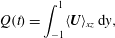 $$\begin{eqnarray}Q(t)=\int _{-1}^{1}\langle \boldsymbol{U}\rangle _{xz}\,\text{d}y,\end{eqnarray}$$
for the two considered Reynolds numbers in this study, i.e.
 $Re=500$
(plotted with a dashed line) and
 $Re=3000$
(solid line) for the problem with time horizon
 $T=5$
, which exhibits typical behaviour for all the problems considered.
(a–c) Variation with
 $y$
and
 $t$
of mean profiles
 $\langle \boldsymbol{U}\rangle _{xz}$
as defined in (3.10) for the transitional flows at
 $Re=3000$
(solid lines) and the parabolic base flow
 $\bar{\boldsymbol{u}}$
(dashed lines). (d–f) Flow rate
 $Q(t)$
as defined in (3.11) for flows with
 $Re=500$
(dashed lines) and
 $Re=3000$
(solid lines) for time horizon
 $T=5$
with optimal initial perturbation, for (d) time-integrated energy growth, (e) mix-norm minimisation and (f) variance minimisation for
 $T=5$
.
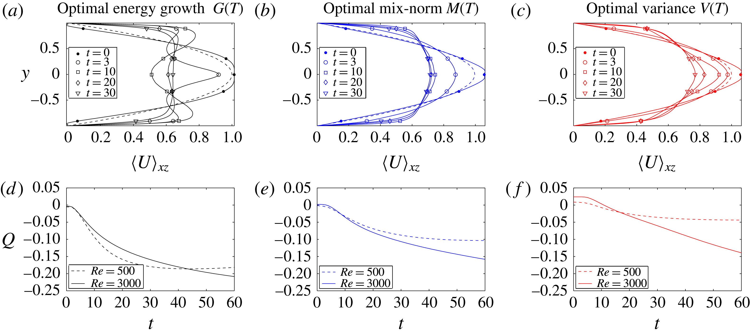
Time evolution of the three studied measures for the three optimisation problems contained in (2.26) at
 $Re=3000$
. For each of the initial perturbations, the rows show: (a,d,g) the time-integrated energy growth
 $G(t)$
; (b,e,h) the mix-norm
 $M(t)$
; and (c,f,i) the variance
 $V(t)$
of the concentration field. The perturbations associated with the different optimisation problems are shown in the columns: (a–c) maximisation of the time-integrated energy growth; (d–f) minimisation of the mix-norm; and (g–i) variance. The quantities
 $G(t)$
,
 $M(t)$
and
 $V(t)$
are defined in (3.5), (3.1) and (3.2), respectively. Thus, the time evolution of the optimal perturbations which actually optimise the specific quantities are shown in the panels located on the diagonal. Each panel contains three plots corresponding to the three chosen time horizons
 $T=2,5,10$
. The associated time horizon for each plot is indicated by a dot. The optimal envelopes
 $G_{opt}^{T}(T)$
,
 $M_{opt}^{T}(T)$
and
 $V_{opt}^{T}(T)$
(plotted with dashed lines) are obtained via cubic interpolation of the optimal values at the time horizons, and the values computed at
 $t=30$
using time horizon
 $T=10$
. The envelopes are plotted in all the panels of each row to allow better comparison between the various optimisation problems. For comparison, the optimal envelopes
 $G_{opt}^{L}(T)$
,
 $M_{opt}^{L}(T)$
and
 $V_{opt}^{L}(T)$
for flows with
 $Re=500$
are plotted with dot-dashed lines.
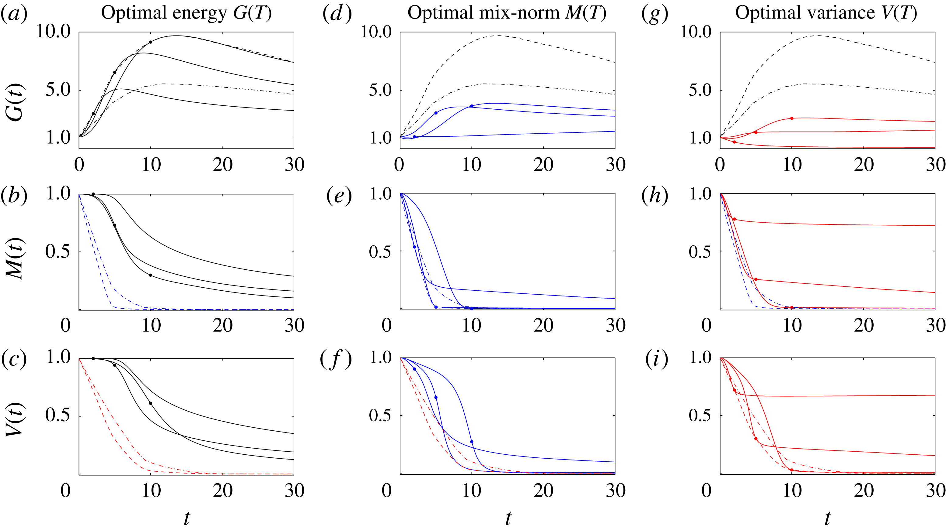
We present the overall results in figure 15, which is organised in the same way as figure 5 for the flows with
 $Re=500$
, i.e. the rows show the time evolution of the key scaled quantities
 $G(t)$
,
 $M(t)$
and
 $V(t)$
as defined in (3.5), (3.1) and (3.2) while the columns correspond to flows determined by solving the three different optimisation problems. Furthermore, the two figures use the same colour coding, in that
 $G(t)$
is plotted in black,
 $M(t)$
is plotted in blue and
 $V(t)$
is plotted in red. The dashed lines mark the different optimal envelopes
 $G_{opt}^{T}$
,
 $M_{opt}^{T}$
and
 $V_{opt}^{T}$
. In order to allow comparison between the flows at the two different Reynolds numbers, we also plot the equivalent optimal envelopes
 $G_{opt}^{L}$
,
 $M_{opt}^{L}$
and
 $V_{opt}^{L}$
(using dot-dashed lines) obtained from flows with
 $Re=500$
. Unsurprisingly, the optimal flows with
 $Re=3000$
reach more extreme values than the equivalent flows with
 $Re=500$
. For example, the maximum energy growth reaches twice the value in the flow with
 $Re=3000$
compared to the flow with
 $Re=500$
. Analogously, mixing, relative to both mix-norm and variance minimisation, is more rapid and complete for
 $Re=3000$
. In particular, the optimal envelopes
 $M_{opt}^{T}$
and
 $V_{opt}^{T}$
become essentially horizontal, corresponding to a state where mixing is occurring at a purely diffusive (asymptotic) rate by
 $t=10$
, thus justifying the chosen time horizons.
Optimal initial conditions for (a) maximising the time-integrated energy growth, (b) minimising the concentration variance and (c) mix-norm for a flow with
 $Re=3000$
over a time horizon
 $T=5$
represented via isosurfaces of 40 % of the maximum (yellow) and minimum (blue) of the streamwise velocity component
 $u$
.
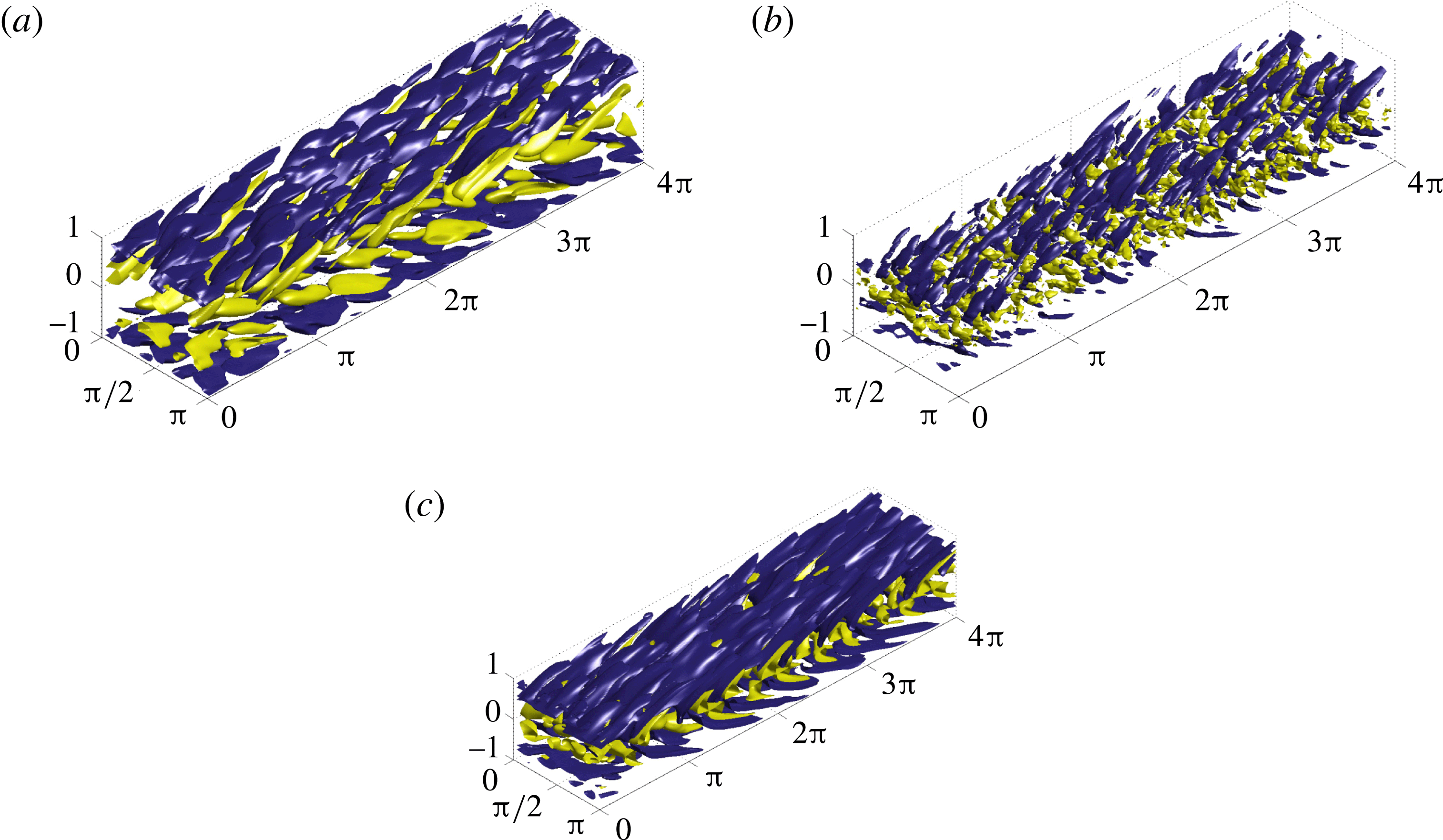
3.3.1 Time-averaged energy-growth maximisation
Similarly to the behaviour for the flows with
 $Re=500$
, the initial perturbations which maximise energy growth form spanwise vortices tilted against the direction of the mean shear allowing energy harvesting via the Orr mechanism. We illustrate the energy-growth optimal perturbation in figure 16(a) by plotting the streamwise velocity component for the perturbation with time horizon
 $T=5$
. Indeed, the initial circulation within the vortices is such that the flux in the central region of the channel is actually increased, which is also shown in the structure of the mean flow profile shown in figure 14(a). As time progresses, with the perturbation vortices being redistributed and reoriented, the mean flow is decelerated in the channel centre while being accelerated closer to the walls giving rise to the boundary layers, leading to a relatively large (transient) energy gain. Consequently, the interface between the two different scalar field concentrations is distorted, with the passive scalar being transported in the wall-normal direction. In figure 17 we plot the time evolution of the concentration field
 $\unicode[STIX]{x1D703}$
for the flow with this initial perturbation. Transition leads to significant mixing in the flow interior at later times, although it is apparent that the passive scalar still remains unmixed in the boundary layers near the walls. Indeed, a quantitative measure of the energy-growth-based mixing is shown in figure 15(c), where the time evolution of
 $V(t)$
for perturbations maximising energy growth can be compared with the (actual) optimal envelope for perturbations which minimise variance, i.e.
 $V_{opt}^{T}$
. Specifically, at time
 $t=30$
(for optimal perturbations with time horizon
 $T=5$
) the energy-growth perturbation has variance three times higher than the equivalent perturbation chosen to minimise variance, demonstrating that, even for such ‘turbulent’ flows, triggering an energetic perturbation is not the ‘best’ way to mix passive scalars in such a shear flow.
Time evolution of the scalar field distribution produced by the energy-growth optimal perturbation (for a flow with
 $Re=3000$
with time horizon
 $T=5$
) plotted in figure 16(a) at (a)
 $t=5$
, (b)
 $t=10$
and (c)
 $t=30$
, on the vertical midplane at
 $z=\unicode[STIX]{x03C0}/2$
(left column) and the horizontal midplane
 $y=0$
(right column).
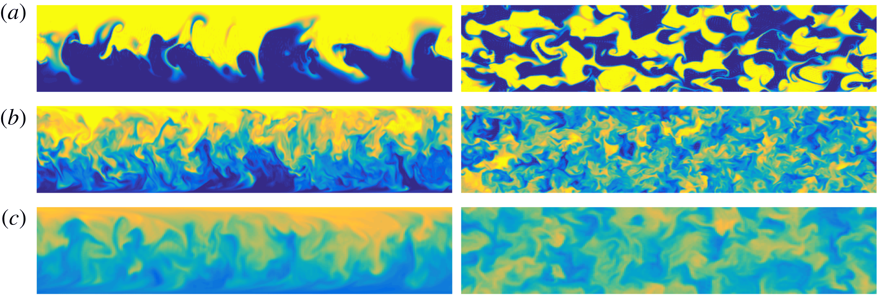
3.3.2 Variance minimisation
The time evolution of the flow induced by the variance-minimising optimal perturbation for
 $Re=3000$
exhibits the same three-stage behaviour (of transport, dispersion and relaxation) as the flow with
 $Re=500$
. Once again, the variance-minimising optimal perturbation comprises small-scale vortices located near the passive scalar interface, as shown in figure 16(b) (for a time horizon
 $T=5$
). It is clear that the characteristic length scales (in both the streamwise and spanwise directions) of the perturbation flow structures are significantly smaller for the variance-minimising optimal perturbation than for the energy-growth-optimal perturbation or for the mix-norm-minimising optimal perturbation over this time horizon. As is typical, the perturbation vortices perturb the interface, extending it towards the channel walls, generating a fine-scale vertically striped pattern in the scalar concentration field. Mixing is then enhanced by the underlying base flow shear, the (intensified) shear in the boundary layers and the spanwise shear, leading to the stripes being smeared out, as shown in figure 18.
Time evolution of the scalar field distribution produced by the variance-minimising optimal perturbation (for a flow with
 $Re=3000$
with time horizon
 $T=5$
) plotted in figure 16(b) at (a)
 $t=5$
, (b)
 $t=10$
and (c)
 $t=30$
, on the vertical midplane at
 $z=\unicode[STIX]{x03C0}/2$
(left column) and the horizontal midplane
 $y=0$
(right column).
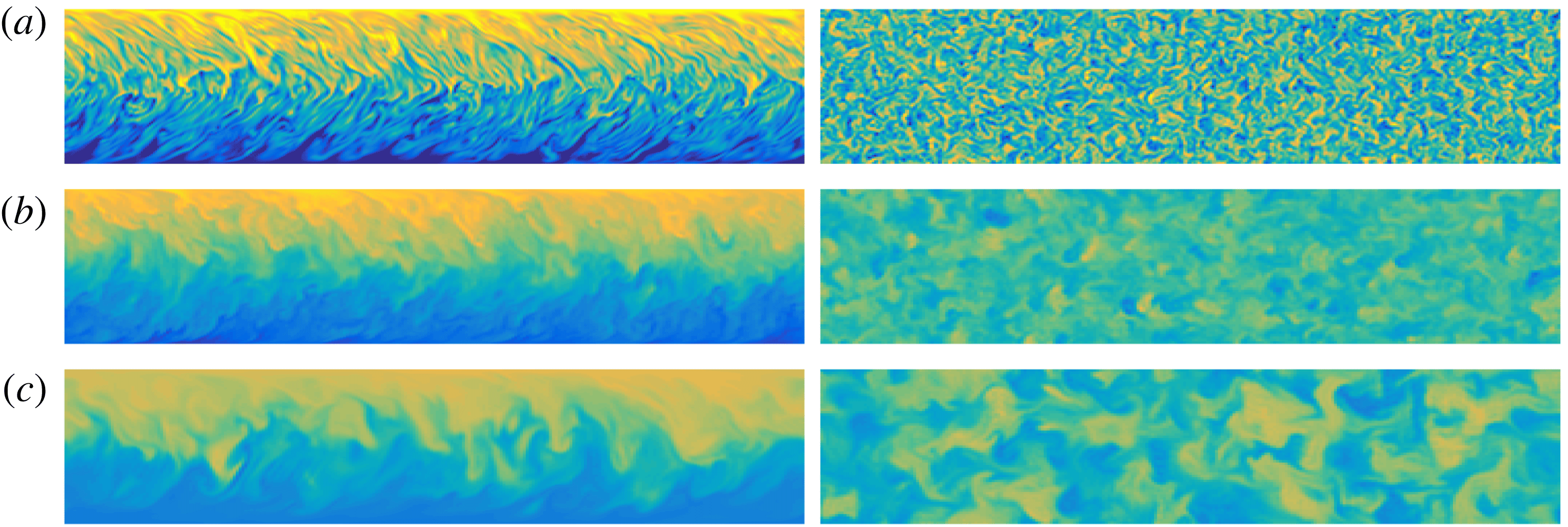
Comparing the envelopes
 $V_{opt}^{L}$
and
 $V_{opt}^{T}$
in figure 15(c), it is apparent that the mixing measures decay only slightly faster for the transitional flow with
 $Re=3000$
than for the flow with
 $Re=500$
. This relatively small difference can be attributed to the growth of the shear in the boundary layers near the channel walls due to the transition to disorder. This is particularly apparent in figure 19, which plots the time evolution of the product terms (3.6)–(3.9) for the optimal variance-minimising perturbation with target time horizon
 $T=10$
in a flow with
 $Re=3000$
. It is apparent that the key qualitative characteristics of the optimal mixing are the same as in the flow with
 $Re=500$
. However, comparing figure 13 with figure 19, it is apparent that the structures have substantially higher amplitude in the flow with
 $Re=3000$
, with, in particular, the boundary layer shear contributing much more intensively to the mixing. As is apparent from consideration of figure 19, the term
 $P_{\bar{u}}$
plays a substantially smaller role, while the term
 $P_{2D}$
dominates. This is in contrast to the behaviour of the flow where
 $Re=500$
, where the various terms are much closer in magnitude, as is apparent in figure 13.
Time and wall-normal variation of the various production terms (as defined in (3.6)–(3.9)) for the variance-optimal flow over a time horizon of
 $T=10$
for a flow with
 $Re=3000$
: (a) the base flow term
 $P_{\bar{u}}$
; (b) the (total) perturbation term
 $P_{u}$
; (c) the perturbation term in the
 $x{-}y$
plane
 $P_{2D}$
; and (d) the three-dimensional deviation term
 $P_{3D}$
.
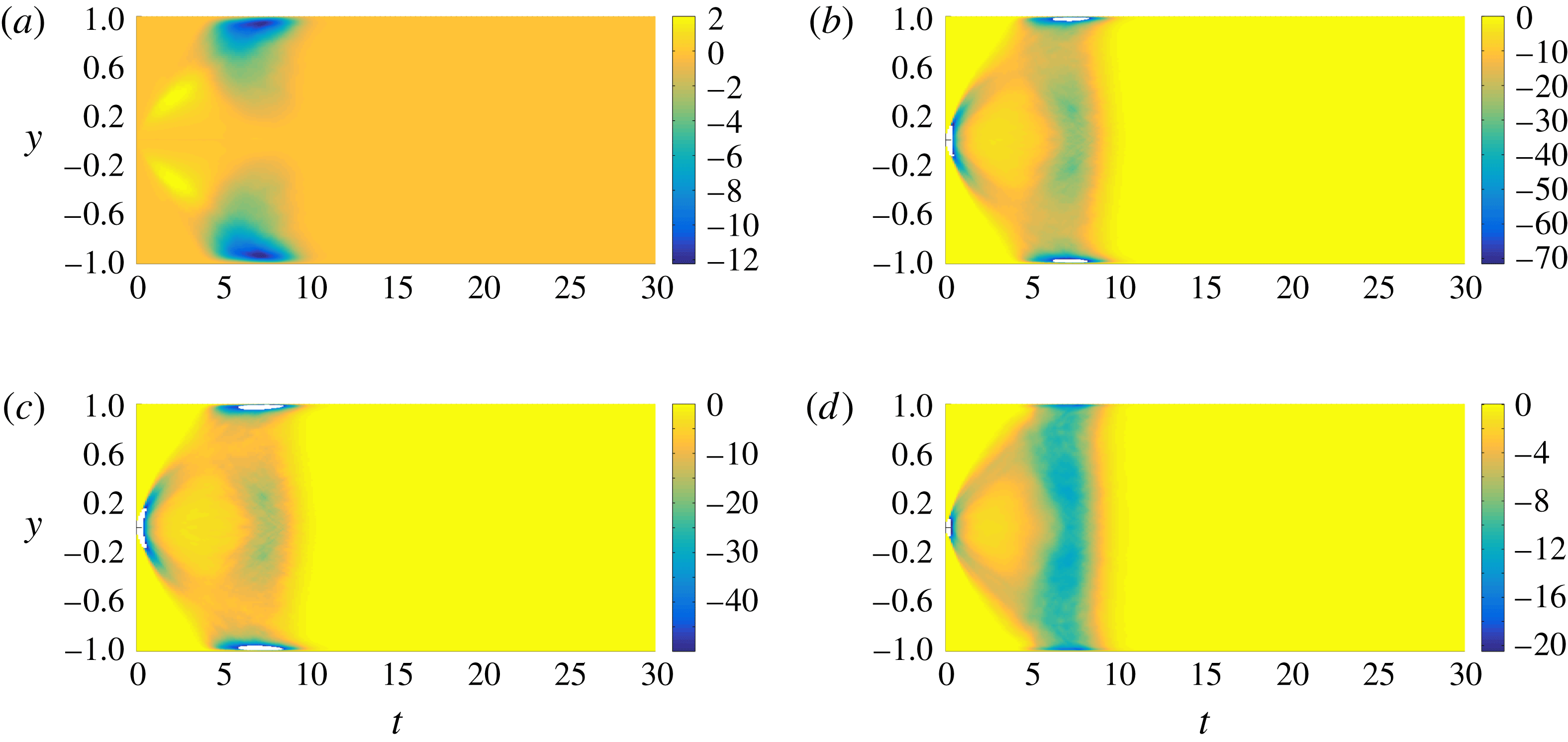
3.3.3 Mix-norm minimisation
Finally, the mix-norm-optimal flow with
 $Re=3000$
largely exhibits the same properties as the equivalent flow with
 $Re=500$
. Similarly to the variance-optimal flow, the perturbations which minimise the mix-norm form vortices tilted against the mean shear direction. As the mix-norm penalises small-scale structures, the characteristic length scale of the mix-norm-minimising vortices is larger than the characteristic length scale of the variance-minimising vortices with the same time horizon for flows with the same
 $Re=3000$
.
However, it is also apparent that the characteristic length scale of these vortices is considerably smaller than the characteristic length scale of the equivalent vortices in the equivalent flow with the same time horizon minimising the mix-norm for flows with
 $Re=500$
. The physical evolution is the same as discussed above, in that the interface between the two initial concentrations is transported towards the channel walls, forming characteristic vertical stripes, which are then dispersed by the enhanced shear, before a final relaxation phase where the concentration field is completely homogenised by molecular diffusion. This time evolution is illustrated in figure 20, where we plot the time evolution of the concentration field under the action of the mix-norm-optimal initial condition for time horizon
 $T=5$
. The associated optimal flow field is presented in figure 16(c).
As in the case of the variance-optimal flows, the increased shear in the near-wall boundary layers at higher
 $Re=3000$
leads to slightly better mixing (in the specific sense of mix-norm minimisation) compared to the equivalent flow at
 $Re=500$
. Unsurprisingly, strong shear is located much closer to the channel walls in the higher-
 $Re$
flow, and so the impact of the wall-induced shear on the reduction in the concentration variance (and mix-norm) is somewhat delayed at higher
 $Re$
. This phenomenon can be observed by comparing the time evolutions of
 $V(t)$
in the mix-norm-optimisation flows with target time
 $T=10$
at the two different Reynolds numbers. Figure 15(f) confirms the usefulness of the mix-norm as a good proxy for the variance. Moreover, we see that, at
 $Re=3000$
, identifying the perturbation which minimises the mix-norm over a relatively short time horizon continues to be better at mixing (i.e. reducing the concentration variance) at late times than the variance-optimal perturbation over the same short time horizon. Considering a specific illustrative example, the optimal perturbation which minimises variance over the time horizon
 $T=5$
has lower variance at the target time
 $T=5$
than the optimal perturbation which minimises the mix-norm at
 $T=5$
. This is unsurprising, since the optimal perturbation which minimises variance is, by construction, designed to minimise variance at the target time, whereas the optimal perturbation which minimises the mix-norm at the target time is not constructed to minimise variance at the target time. However, as time increases beyond the target time, the decay of variance driven by the variance-optimal perturbation slows down considerably, while for the mix-norm-optimal initial perturbation the variance continues to decay rapidly until its value approaches the optimal envelope.
Time evolution of the scalar field distribution produced by the mix-norm-optimal perturbation (for a flow with
 $Re=3000$
with time horizon
 $T=5$
) plotted in figure 16(a) at (a)
 $t=5$
, (b)
 $t=10$
and (c)
 $t=30$
, on the vertical midplane at
 $z=\unicode[STIX]{x03C0}/2$
(left column) and the horizontal midplane
 $y=0$
(right column).
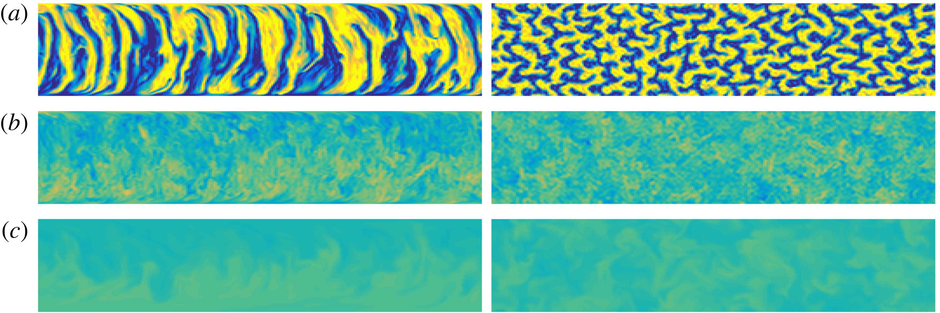
In summary, unsurprisingly, the solutions of the optimisation problem (2.26) for flows with
 $Re=3000$
differ in detail from those for flows with
 $Re=500$
, although our analysis shows that the key conclusions drawn from the properties of the flows with
 $Re=500$
carry over to the flows with
 $Re=3000$
. We now turn our attention to attempting to quantify some appropriate measure of the ‘efficiency’ of the mixing induced by the various optimal perturbations.
3.4 Mixing performance
In simple terms, the ‘performance’ of a process may be defined as the ratio between the quantity of some required outcome to some appropriate measure of the ‘cost’ of the process. Here, we choose to define the ‘performance’ of the mixing through some desirable measure of the mixing (capturing both the quality and quantity of mixing) scaled by the energy consumption of the mixing process, i.e.
 $$\begin{eqnarray}\displaystyle \text{mixing performance}=\frac{\text{mixing measure}}{\text{ energy consumed }}=\frac{{\mathcal{M}}_{{\mathcal{P}}}}{{\mathcal{E}}_{{\mathcal{C}}}}. & & \displaystyle\end{eqnarray}$$
As the flows that we consider are inherently time-dependent, it is natural to define the mixing performance of a given flow as the ratio of the amount of fluid mixed (as measured in terms of an appropriately defined mixing measure over a time interval
 $[0,t]$
relative to the energy consumed over the same period of time.
The mixing measure quantity
 ${\mathcal{M}}_{{\mathcal{P}}}$
in the numerator of (3.12) should be defined as a function which monotonically increases with some appropriate measure of the quality of the resulting mixture as well as the amount of fluid mixed. From a physical perspective, the concentration variance is the most natural description of mixture quality, and so for the purpose of this section we regard it as the mixing measure. We thus define
 ${\mathcal{M}}_{{\mathcal{P}}}$
over a given time interval
 $[0,t]$
as
 $$\begin{eqnarray}\displaystyle {\mathcal{M}}_{{\mathcal{P}}}(t)=\int _{0}^{t}[Q(s)(1-V(s))]\,\text{d}s, & & \displaystyle\end{eqnarray}$$
where the variable
 $Q$
is the mean flow rate through the channel as defined in (3.11) and
 $V$
is the variance of the concentration field, scaled by the purely diffusive variance
 $\unicode[STIX]{x1D703}_{d}(t)$
, as defined in (3.2).
In theory (Paul, Atiemo-Obeng & Kresta Reference Paul, Atiemo-Obeng and Kresta2004), in an equilibrium state the power delivered to the system is equivalent to that lost or dissipated in the fluid. Naturally, in transitional flows, energy dissipation increases, which is manifest by an increase in the friction factor (Bergman et al.
Reference Bergman, Incropera, DeWitt and Lavine2011), leading inevitably to a decrease in the mean flow rate for a constant imposed pressure gradient. Therefore,
 $\text{d}Q(t)/\text{d}t$
can be used as an appropriate measure of the energy consumption
 ${\mathcal{E}}_{{\mathcal{C}}}$
by the mixing processes in (3.11). However, for the flows that we are considering here, the picture is complicated by the fact that
 $Q(t)$
varies non-monotonically, as is apparent in figure 14. Therefore, it is mathematically convenient to capture the change of the mean flow rate relative to a reference flow rate
 $Q_{ref}$
via an integral measure
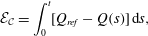 $$\begin{eqnarray}\displaystyle {\mathcal{E}}_{{\mathcal{C}}}=\int _{0}^{t}[Q_{ref}-Q(s)]\,\text{d}s, & & \displaystyle\end{eqnarray}$$
which avoids the denominator of the expression for the mixing ‘performance’ being zero. It is important to remember that the initial perturbation actually injects a fixed amount of energy into the flow, and so the appropriate reference flow rate
 $Q_{ref}$
is the maximal initial flow rate associated with a flow perturbation that satisfies the energy constraint (2.23), i.e.
 $$\begin{eqnarray}\displaystyle Q_{ref}=\max _{\Vert \boldsymbol{u}_{0}(\boldsymbol{x})\Vert _{L^{2}(\unicode[STIX]{x1D6FA})}^{2}=2e_{0}|\unicode[STIX]{x1D6FA}|}\int _{-1}^{1}\langle \bar{\boldsymbol{u}}+\boldsymbol{u}_{0}\rangle _{xz}\,\text{d}y. & & \displaystyle\end{eqnarray}$$
Since the flow rate is maximised when the perturbation is purely in the streamwise direction, we find that
 $\boldsymbol{u}_{0}=\sqrt{3/8}\,(1-y^{2})\boldsymbol{e}_{\boldsymbol{x}}$
and so
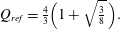 $$\begin{eqnarray}\displaystyle Q_{ref}={\textstyle \frac{4}{3}}\Big(1+\sqrt{{\textstyle \frac{3}{8}}}\,\Big). & & \displaystyle\end{eqnarray}$$
Therefore, we define an appropriate mixing ‘performance’ as
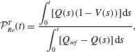 $$\begin{eqnarray}\displaystyle {\mathcal{P}}_{Re}^{T}(t)=\frac{\displaystyle \int _{0}^{t}[Q(s)(1-V(s))]\,\text{d}s}{\displaystyle \int _{0}^{t}[Q_{ref}-Q(s)]\,\text{d}s}, & & \displaystyle\end{eqnarray}$$
where the superscript
 $T$
denotes the target time horizon.
Time evolution of the mixing performance
 ${\mathcal{P}}_{Re}^{T}$
as defined in (3.17) for flows with (a)
 $Re=500$
and (b)
 $Re=3000$
and which maximise integrated energy growth (thin black dotted lines), minimise mix-norm (blue dashed lines) and minimise variance (red full lines). Flows associated with different target times are distinguished by different markers.
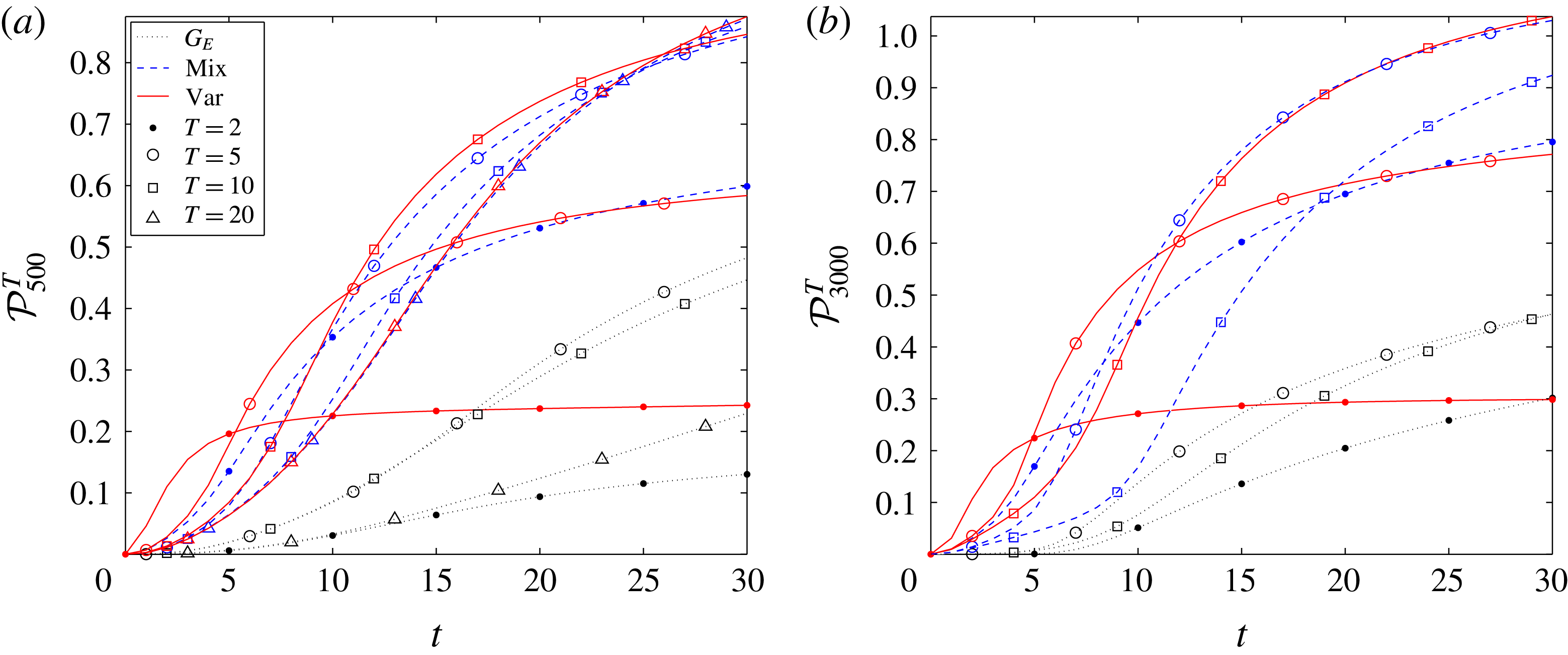
Figure 21 shows the time evolution of this mixing performance
 ${\mathcal{P}}_{Re}^{T}$
for the two considered flow regimes. We see that, consistently with the above discussion, the mixing strategy based on maximising the time-integrated energy growth is outperformed by the other strategies because it both uses more energy (suppressing the flow rate) and, for all target times, produces comparatively poorer decay of concentration variance. In fact, except for the variance minimisation on the shortest target time
 $T=2$
, both minimisation strategies are more efficient than the energy-growth amplification for all tested target times irrespective of the choice of Reynolds number. Indeed, using this particular measure
 ${\mathcal{P}}_{Re}^{T}$
, the perturbations which minimise either the concentration variance or the mix-norm for flows with
 $Re=500$
have better mixing performance than the energy-growth-optimising perturbations for flows with
 $Re=3000$
.
For the variance-minimising mixing strategies, increasing the Reynolds number (and hence triggering transition) increases the mixing performance, in that
 ${\mathcal{P}}_{500}^{T}(t)<{\mathcal{P}}_{3000}^{T}(t)$
for all times
 $t$
and for any chosen target time
 $T$
. This is also the case for the mix-norm-minimising strategy when the target time is short (e.g.
 $T=2,5$
). For longer target times, the flows with smaller Reynolds number actually exhibit superior performance at early times since the wall-induced shear is less localised near the walls and thus reached earlier by the interface between the two concentrations being transported from the centre of the channel. An example of this phenomenon occurs for the flows with target time
 $T=10$
, for which
 ${\mathcal{P}}_{500}^{10}(t)\geqslant {\mathcal{P}}_{3000}^{10}(t)$
up to
 $t\lesssim 15$
.
Contrasting the two minimisation strategies, it is apparent that the variance-minimising strategy has higher performance for short times. This is because, for a given target time, the optimal variance-minimising perturbations both mix more thoroughly and dissipate less energy, as is apparent through comparison of panels (d) and (g) in figures 5 and 15. However, for longer times, despite dissipating more energy, the optimal mix-norm-minimising perturbations prove to have higher performance, essentially because they continue to drive mixing even beyond the chosen optimisation horizon. This is particularly noticeable in the transitional flows with
 $Re=3000$
, where the mix-norm-based strategy for a target time
 $T=5$
delivers almost the same performance as the variance-based strategy with
 $T=10$
. This behaviour, which is also superior to the mix-norm-based strategy with longer target time
 $T=10$
, can be understood by consideration of figure 15(f). As shown in that figure, the later time behaviour of the variance for the mix-norm-minimising flow with
 $T=5$
very closely approaches the optimal envelope
 $V_{opt}^{T}$
of the time evolution of the various variance-minimising flows, demonstrating that the two flows should be expected to be very similar in their mixing performance. However, the variance for the mix-norm minimising flow with
 $T=10$
actually does not approach this envelope as closely, suggesting strongly that the ensuing mixing is not ultimately as thorough, consistently with the inferior mixing performance shown in figure 21(b).
Of course, the flows at higher Reynolds number inevitably have a much higher imposed pressure gradient. Therefore, at least from an engineering point of view, it is extremely important to investigate whether the improvement in mixing performance at higher flow rates outweighs the actual (dimensional) extra power needed to drive the flow. To address this issue, it is more appropriate to base the mixing performance on the total energy utilised to drive the flow and the total amount of fluid mixed. Therefore, the definition of the appropriate mixing performance (3.12) needs to be modified, as it is necessary to consider dimensional quantities, essentially because the time scale embedded in the non-dimensionalisation is scaled with the (dimensional) characteristic flow velocity.
Hence, we consider the dimensional work done by the constant base pressure gradient on the flow
 $U^{\ast }$
, i.e.
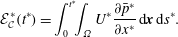 $$\begin{eqnarray}\displaystyle {\mathcal{E}}_{{\mathcal{C}}}^{\ast }(t^{\ast })=\int _{0}^{t^{\ast }}\!\!\int _{\unicode[STIX]{x1D6FA}}U^{\ast }\frac{\unicode[STIX]{x2202}\bar{p}^{\ast }}{\unicode[STIX]{x2202}x^{\ast }}\,\text{d}\boldsymbol{x}\,\text{d}s^{\ast }. & & \displaystyle\end{eqnarray}$$
In addition, to measure the mixing performance we use the total amount of fluid mixed during the time interval
 $[0,t^{\ast }]$
 $$\begin{eqnarray}\displaystyle {\mathcal{M}}_{{\mathcal{P}}}^{\ast }(t^{\ast })=\unicode[STIX]{x03C0}h^{\ast }\unicode[STIX]{x1D70C}^{\ast }\int _{0}^{t^{\ast }}[Q^{\ast }(s^{\ast })(1-V(s^{\ast }))]\,\text{d}s^{\ast }, & & \displaystyle\end{eqnarray}$$
where the mean flow rate
 $Q^{\ast }$
is defined in (3.11). Altogether, we introduce an alternative (dimensional) mixing performance
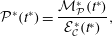 $$\begin{eqnarray}\displaystyle {\mathcal{P}}^{\ast }(t^{\ast })=\frac{{\mathcal{M}}_{{\mathcal{P}}}^{\ast }(t^{\ast })}{{\mathcal{E}}_{{\mathcal{C}}}^{\ast }(t^{\ast })}, & & \displaystyle\end{eqnarray}$$
remembering that the asterisks in equations (3.18)–(3.20) denote dimensional variables.
The mixing performances in
 $Re=500$
and
 $Re=3000$
then need to be assessed with consideration to the scaling introduced in § 2 since the key time scale
 $\unicode[STIX]{x1D70F}^{\ast }=h^{\ast }/U_{m}^{\ast }$
differs in the two studied flow regimes. The true comparison of the mixing performance
 ${\mathcal{P}}^{\ast }(t^{\ast })$
can only be done with respect to the same time units. Taking advantage of the scaling introduced in § 2.2, we can thus re-pose the mixing performance as
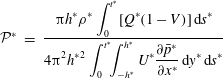 $$\begin{eqnarray}\displaystyle {\mathcal{P}}^{\ast } & = & \displaystyle \frac{\displaystyle \unicode[STIX]{x03C0}h^{\ast }\unicode[STIX]{x1D70C}^{\ast }\int _{0}^{t^{\ast }}[Q^{\ast }(1-V)]\,\text{d}s^{\ast }}{\displaystyle 4\unicode[STIX]{x03C0}^{2}{h^{\ast }}^{2}\int _{0}^{t^{\ast }}\!\!\int _{-h^{\ast }}^{h^{\ast }}U^{\ast }\frac{\unicode[STIX]{x2202}\bar{p}^{\ast }}{\unicode[STIX]{x2202}x^{\ast }}\,\text{d}y^{\ast }\,\text{d}s^{\ast }}\end{eqnarray}$$
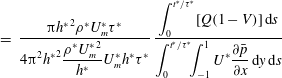 $$\begin{eqnarray}\displaystyle & = & \displaystyle \frac{\unicode[STIX]{x03C0}{h^{\ast }}^{2}\unicode[STIX]{x1D70C}^{\ast }U_{m}^{\ast }\unicode[STIX]{x1D70F}^{\ast }}{\displaystyle 4\unicode[STIX]{x03C0}^{2}{h^{\ast }}^{2}\frac{\unicode[STIX]{x1D70C}^{\ast }{U_{m}^{\ast }}^{2}}{h^{\ast }}U_{m}^{\ast }h^{\ast }\unicode[STIX]{x1D70F}^{\ast }}\,\frac{\displaystyle \int _{0}^{t^{\ast }/\unicode[STIX]{x1D70F}^{\ast }}[Q(1-V)]\,\text{d}s}{\displaystyle \int _{0}^{t^{\ast }/\unicode[STIX]{x1D70F}^{\ast }}\!\!\int _{-1}^{1}U^{\ast }\frac{\unicode[STIX]{x2202}\bar{p}}{\unicode[STIX]{x2202}x}\,\text{d}y\,\text{d}s}\end{eqnarray}$$
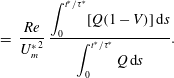 $$\begin{eqnarray}\displaystyle & = & \displaystyle \frac{Re}{{U_{m}^{\ast }}^{2}}\,\frac{\displaystyle \int _{0}^{t^{\ast }/\unicode[STIX]{x1D70F}^{\ast }}[Q(1-V)]\,\text{d}s}{\displaystyle \int _{0}^{t^{\ast }/\unicode[STIX]{x1D70F}^{\ast }}Q\,\text{d}s}.\end{eqnarray}$$
We see that mixing performances in the two flow classes are thus determined by the time evolution of
 $V$
and
 $Q$
, as well as the factor
 $Re/{U_{m}^{\ast }}^{2}$
, where
 $U_{m}^{\ast }$
is the (maximum) centreline velocity as used in § 2.2.
In order to compare the mixing performances at
 $Re=500$
and
 $Re=3000$
, let us select the time scale
 $\unicode[STIX]{x1D70F}^{\ast }$
to be the one implied for the flow with
 $Re=500$
. Thus, for the case that is most relevant to engineering, where the Reynolds number is controlled by the flow velocity, we can introduce two scaled mixing performances as
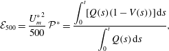 $$\begin{eqnarray}\displaystyle & \displaystyle {\mathcal{E}}_{500}=\frac{{U_{m}^{\ast }}^{2}}{500}\,{\mathcal{P}}^{\ast }=\frac{\displaystyle \int _{0}^{t}[Q(s)(1-V(s))]\,\text{d}s}{\displaystyle \int _{0}^{t}Q(s)\,\text{d}s}, & \displaystyle\end{eqnarray}$$
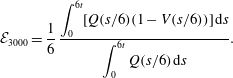 $$\begin{eqnarray}\displaystyle & \displaystyle {\mathcal{E}}_{3000}=\frac{1}{6}\,\frac{\displaystyle \int _{0}^{6t}[Q(s/6)(1-V(s/6))]\,\text{d}s}{\displaystyle \int _{0}^{6t}Q(s/6)\,\text{d}s}. & \displaystyle\end{eqnarray}$$
Note that in (3.24) the non-dimensional functions
 $V$
and
 $Q$
denote scaled variance and mean flow rate computed for flows with
 $Re=500$
, whereas in (3.25) they represent the same variables obtained from simulations for flows with
 $Re=3000$
.
We plot the time evolution of
 ${\mathcal{E}}_{500}$
and
 ${\mathcal{E}}_{3000}$
in figure 22 for the various mixing strategies and time horizons. Consistently with all other results, the performance of the energy-growth-based mixing strategy is least effective when assessed with these measures of mixing performance. For short time intervals, the variance-based mixing strategy uses the energy input more effectively than the mix-norm-based strategy. However, for longer time intervals, the mix-norm-based strategy has a higher mixing performance. Notably, for flows with
 $Re=3000$
, the perturbation which minimises the mix-norm at the target time
 $T=5$
has the best mixing performance out of all the studied strategies. Direct comparisons of mixing performances are shown in figure 22 where
 ${\mathcal{E}}_{500}$
and
 ${\mathcal{E}}_{3000}$
are plotted for the various time horizons and mixing strategies. From the initial rate of change of the mixing performance measures, it is clear that mixing for flows with
 $Re=3000$
occurs significantly faster than for flows with
 $Re=500$
. From the fact that
 $M_{opt}^{L}<M_{opt}^{T}$
and
 $V_{opt}^{L}<V_{opt}^{T}$
, mixing changes with
 $Re$
faster than at a purely linear rate. However, this faster mixing requires a larger amount of energy than is needed to drive the flow down the channel. In particular, comparing the end values of
 ${\mathcal{E}}_{500}$
and
 ${\mathcal{E}}_{3000}$
shows that the (dimensional) mixing performance is approximately five times higher for flows with
 $Re=500$
compared to flows with
 $Re=3000$
.
Time evolution of scaled mixing performances (a)
 ${\mathcal{E}}_{500}$
and (b)
 ${\mathcal{E}}_{3000}$
as defined in (3.24) and (3.25) for flows which maximise integrated energy growth (thin black dotted lines), minimise mix-norm (blue dashed lines) and minimise variance (red lines). Flows associated with different target times are distinguished by different markers.
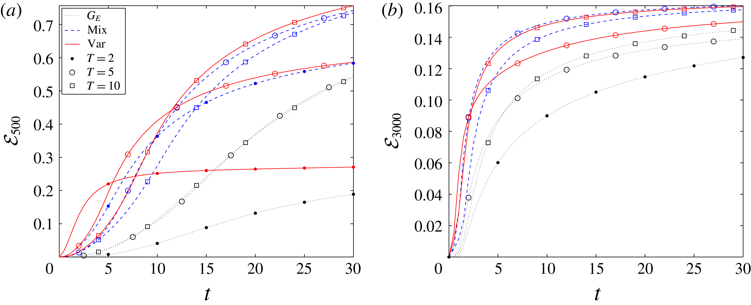
4 Conclusions
We have studied mixing of a passive scalar in pressure-driven plane Poiseuille flow. Our objective was to identify optimal initial perturbations (of a fixed, non-trivial energy) to the laminar parabolic flow that result, at some chosen time horizon, in maximal mixing of the passive scalar. We consider physically realistic, incompressible flows so that the velocity field and pressure satisfy the Navier–Stokes equations and the continuity equation, while the concentration field of the passive scalar is governed by an advection–diffusion equation. We have restricted attention to flows with Schmidt number
 $Sc\equiv \unicode[STIX]{x1D708}^{\ast }/\unicode[STIX]{x1D705}^{\ast }=1$
and two qualitatively different Reynolds numbers:
 $Re=500$
and
 $Re=3000$
. Three different optimisation problems have been considered: the maximisation of the time-integrated energy growth; minimisation of the mix-norm (Mathew et al.
Reference Mathew, Mezi and Petzold2005; Thiffeault Reference Thiffeault2012); and minimisation of the concentration variance. The mathematical formulation of these problems yields constrained minimisation problems, which we solve numerically using a nonlinear direct-adjoint-looping (DAL) method.
We have revisited and reassessed pre-existing hypotheses presented in the literature regarding the best strategy for mixing. A classic hypothesis due to Aamo & Krstić (Reference Aamo and Krstić2003) is that the development of the complex flow patterns which accompany turbulence transition leads to highly effective and thorough mixing. On the other hand, Foures et al. (Reference Foures, Caulfield and Schmid2014) showed, through a sequence of two-dimensional numerical simulations for flows with relatively modest
 $Re=500$
, that the perturbations which experience the largest transient energy growth, and which might be considered to be the ones which would trigger turbulence ultimately, lead to relatively poor mixing. Instead, a different mixing strategy was identified using the direct-adjoint-looping (DAL) method. This strategy exploits so-called Taylor dispersion as the key (intermediate) stirring mechanism. Our reassessment generalises the approach of Foures et al. (Reference Foures, Caulfield and Schmid2014) to three-dimensional flows both at the same modest Reynolds number
 $Re=500$
, and at a significantly larger
 $Re=3000$
, where the perturbed flow actually exhibits transition to highly disordered, turbulent flow.
Using the DAL method, we consider the three different optimisation problems at various target times. For flows with
 $Re=500$
we find that the time-integrated energy-growth-maximising perturbations lead to a larger decrease in the concentration variance than was found by Foures et al. (Reference Foures, Caulfield and Schmid2014), a difference we attribute to the inherent three-dimensionality of the problem. Nevertheless, the key observation of Foures et al. (Reference Foures, Caulfield and Schmid2014) remains: the most unstable perturbations are sub-optimal if the objective is to homogenise the initially layered scalar concentration distribution. Furthermore, and perhaps more significantly, this observation continues to apply to the flows with
 $Re=3000$
. Although the complicated nonlinear flow structures associated with transition to turbulence reduce the concentration variance in the bulk flow, the passive scalar still remains largely unmixed in the near-wall boundary layers of the channel. For energy-growth maximisation within the time interval
 $t\in [0,30]$
(scaled with advective units) considered here, the best mixing (defined in terms of the variance at
 $t=30$
) is actually achieved in the flow with
 $Re=500$
with the optimal energy-growth perturbation for
 $T=10$
. For this particular flow, the variance of the concentration field decays to
 ${\sim}5\,\%$
of its initial value at
 $t=30$
.
The sub-optimality of this mixing can be put into context by consideration of the optimisation problems that determine the initial perturbations leading to minimisation of the variance at the target time. We find that, within the same time interval
 $t\in [0,30]$
, the variance can be reduced by appropriate optimal perturbations to
 ${\sim}0.02\,\%$
of its initial value. Moreover, high levels of homogeneity are produced for times
 $t\gtrsim 10$
, and increasing
 $Re$
leads to only a relatively slight improvement in the mixing.
Furthermore, similarly to the two-dimensional flows considered by Foures et al. (Reference Foures, Caulfield and Schmid2014), the mixing strategy associated with the optimal variance-minimising perturbations dynamically evolves through the three stages described by Foures et al. (Reference Foures, Caulfield and Schmid2014), in that the concentration field is ‘transported’, ‘dispersed’ and then ‘relaxed’ towards homogeneity. The interface between the two regions of initially different concentration is first stretched and transported from the centreline of the channel towards the walls where the shear is stronger. Since the flow has a finite Péclet number, irreversible mixing via molecular diffusion still acts on a progressively larger interface. The interface is then dispersed and mixing is further enhanced due to the action of the velocity shear. As we demonstrate, there are three contributions to this shear dispersion: shear due to the base parabolic flow; shear due to wall-normal variation of the (perturbed) streamwise velocity; and an inherently three-dimensional component associated with spatial variability of the spanwise velocity.
As previously identified by Foures et al. (Reference Foures, Caulfield and Schmid2014), in two-dimensional flows, the significant shear is predominantly associated with the (laminar) base flow, and so Taylor dispersion represents the key physical mechanism driving the (optimal) mixing. Significantly, when the flow is allowed to evolve in three dimensions at
 $Re=500$
, these three contributions are of approximately the same magnitude, and the temporal evolution of the optimal perturbation exploits all three contributions in suitable combination. Finally, the last ‘relaxation’ stage is characterised by decay of both perturbation energy and concentration variance due to the molecular diffusion.
For
 $Re=3000$
this three-stage picture of the optimal mixing strategy is conceptually very similar. The principal difference associated with the increase in the Reynolds number of the flow appears to arise in the intermediate ‘dispersion’ phase, as the (perturbed) shear available for mixing enhancement in the boundary layers is much stronger in this transitional flow, and so this contribution dominates the mixing during this intermediate phase. It appears that this is the principal reason why mixing at higher
 $Re$
is more rapid.
Moreover, we study the evolution of flows initialised with perturbations optimised to minimise the value of the ‘mix-norm’ at the target time. We find that the time evolution of the variance for such flows actually closely follows the behaviour of flows initialised with perturbations optimised to minimise the variance at relatively long target times, to the extent that the mix-norm and variance-optimal envelopes coincide for late times. For flows with
 $Re=500$
, we find, consistently with the two-dimensional results of Foures et al. (Reference Foures, Caulfield and Schmid2014), that for sufficiently long target times, such as
 $T=20$
, the mix-norm-optimal perturbations converge in structure to the perturbations minimising the variance.
Crucially, and particularly usefully for computational reasons, we find that the mix-norm-optimal perturbations are less sensitive to the choice of the target horizon than the variance-optimal perturbations. This observation has two important consequences. Firstly, optimal perturbations which minimise the mix-norm for short time horizons result in better mixing (i.e. lower concentration variance) at late times than optimal perturbations which minimise the variance for the same (short) time horizon. Secondly, such short-time-horizon mix-norm-minimising perturbations can lead to thorough mixing close to that achieved by long-time-horizon variance-minimising perturbations, which are substantially more expensive to compute, both because the time ‘loop’ is longer, and because the rate of decay of variance is typically slower than the decay of the mix-norm, particularly at early times. These highly useful computational properties are particularly prominent for flows with
 $Re=500$
but are also manifest in the flows with higher
 $Re=3000$
. Altogether, we conclude that the mix-norm is a practicable yet mathematically consistent measure of mixing and its minimisation represents a computationally convenient algorithm to identify a robust mixing strategy.
Finally, we considered appropriate measures of the ‘mixing performance’ at the two studied Reynolds numbers. Unsurprisingly, the transitional flows with
 $Re=3000$
reached more homogeneous concentration distributions (measured either with the mix-norm or the variance) more quickly than the flows with
 $Re=500$
. In terms of the relative energy loss of the flow, the higher-Reynolds-number flow exhibits better performance. However, relative to the total mechanical work done by the pressure gradient which drives the fluid through the channel, the higher-
 $Re$
flow requires much more energy input than the lower-
 $Re$
flow to mix the same quantity of fluid to the same level. Therefore, at least in terms of total energy consumption, the higher-
 $Re$
flow exhibits a poorer mixing performance.
This observation, allied to the clear evidence that perturbations which maximise energy growth are actually strongly sub-optimal for mixing, calls into question conventional wisdom concerning the best way to mix fluids of different composition effectively. The DAL method is clearly well-suited to explore this issue further, and to identify optimal mixing strategies in more realistic situations, with, for example, time-dependent forcing and finite-residence-time flows with natural inflow–outflow conditions, as it naturally allows the algorithmic identification of ‘optimal’ mixing strategies.
Acknowledgements
Thanks are due to the anonymous referees, whose thoughtful and constructive comments have substantially improved this paper. This work was supported by the UK Engineering and Physical Sciences Research Council (EPSRC) grant EP/H023348/1 for the University of Cambridge Centre for Doctoral Training, the Cambridge Centre for Analysis. The research activity of C.P.C. is supported by EPSRC Programme grant EP/K034529/1 entitled ‘Mathematical Underpinnings of Stratified Turbulence’. This research was also supported in part by the National Science Foundation under grant no. NSF PHY17-48958. The hospitality of the Kavli Institute of Theoretical Physics (KITP) at the University of California, Santa Barbara, during the TRANSTURB17 programme is gratefully acknowledged. Data used to create figures 3, 5, 6, 8, 11, 13–16, 19 and 21–24 and the initial condition header data for Diablo for the various simulations are available at https://doi.org/10.17863/CAM.22239.
Appendix A. Necessary conditions for optimality
In § 2 we introduced the optimal initial value problem for mixing:
 $$\begin{eqnarray}\displaystyle \underset{\Vert \boldsymbol{u}_{0}\Vert _{L^{2}}^{2}=2e_{0}|\unicode[STIX]{x1D6FA}|}{\operatorname{argmin}}\{{\mathcal{J}}(\boldsymbol{u}(T),\unicode[STIX]{x1D703}(T))\mid (\boldsymbol{u},\unicode[STIX]{x1D703})\in {\mathcal{N}}{\mathcal{S}}_{u_{0}}^{div}\times {\mathcal{A}}{\mathcal{D}}_{\unicode[STIX]{x1D703}_{0}}\}. & & \displaystyle\end{eqnarray}$$
The iterative scheme for solving (A 1), which is formulated in § 2.3, is based on finding a local minimum of the augmented functional
 $$\begin{eqnarray}\displaystyle & & \displaystyle {\mathcal{L}}(\boldsymbol{u}_{0},\boldsymbol{u},\unicode[STIX]{x1D703},p,\boldsymbol{u}_{0}^{\dagger },\boldsymbol{u}^{\dagger },\unicode[STIX]{x1D703}^{\dagger },p^{\dagger },\!)\nonumber\\ \displaystyle & & \displaystyle \quad ={\mathcal{J}}(\boldsymbol{u},\unicode[STIX]{x1D703})-{\mathcal{J}}_{{\mathcal{N}}{\mathcal{S}}}(\boldsymbol{u},p,\boldsymbol{u}^{\dagger })-{\mathcal{J}}_{{\mathcal{A}}{\mathcal{D}}}(\unicode[STIX]{x1D703}^{\dagger },\unicode[STIX]{x1D703},\boldsymbol{u})-{\mathcal{J}}_{{\mathcal{C}}}(p^{\dagger },\boldsymbol{u})-{\mathcal{J}}_{{\mathcal{I}}{\mathcal{C}}}(\boldsymbol{u}_{0},\boldsymbol{u},\boldsymbol{u}_{0}^{\dagger }),\end{eqnarray}$$
where the summands written in the component notation are
 $$\begin{eqnarray}\displaystyle & \displaystyle {\mathcal{J}}=-\frac{1-\unicode[STIX]{x1D6FC}}{2}\int _{0}^{T}\!\!\int _{\unicode[STIX]{x1D6FA}}u_{i}u_{i}\,\text{d}\boldsymbol{x}+\frac{\unicode[STIX]{x1D6FC}}{2}\int _{\unicode[STIX]{x1D6FA}}\unicode[STIX]{x2202}_{i}^{-\unicode[STIX]{x1D6FD}}\unicode[STIX]{x1D703}(\boldsymbol{x},T)\unicode[STIX]{x2202}_{i}^{-\unicode[STIX]{x1D6FD}}\unicode[STIX]{x1D703}(\boldsymbol{x},T)\,\text{d}\boldsymbol{x}, & \displaystyle\end{eqnarray}$$
 $$\begin{eqnarray}\displaystyle & \displaystyle {\mathcal{J}}_{{\mathcal{N}}{\mathcal{S}}}=\int _{0}^{T}\!\!\int _{\unicode[STIX]{x1D6FA}}u_{i}^{\dagger }(\unicode[STIX]{x2202}_{t}u_{i}+U_{j}\unicode[STIX]{x2202}_{j}u_{i}+u_{j}\unicode[STIX]{x2202}_{j}\bar{u}_{i}+\unicode[STIX]{x2202}_{i}p-Re^{-1}\unicode[STIX]{x2202}_{jj}^{2}u_{i})\,\text{d}\boldsymbol{x}, & \displaystyle\end{eqnarray}$$
 $$\begin{eqnarray}\displaystyle & \displaystyle {\mathcal{J}}_{{\mathcal{A}}{\mathcal{D}}}=\int _{0}^{T}\!\!\int _{\unicode[STIX]{x1D6FA}}\unicode[STIX]{x1D703}^{\dagger }(\unicode[STIX]{x2202}_{t}\unicode[STIX]{x1D703}+U_{j}\unicode[STIX]{x2202}_{j}\unicode[STIX]{x1D703}-Pe^{-1}\unicode[STIX]{x2202}_{jj}^{2}\unicode[STIX]{x1D703})\,\text{d}\boldsymbol{x}\,\text{d}t, & \displaystyle\end{eqnarray}$$
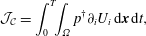 $$\begin{eqnarray}\displaystyle & \displaystyle {\mathcal{J}}_{{\mathcal{C}}}=\int _{0}^{T}\!\!\int _{\unicode[STIX]{x1D6FA}}p^{\dagger }\unicode[STIX]{x2202}_{i}U_{i}\,\text{d}\boldsymbol{x}\,\text{d}t, & \displaystyle\end{eqnarray}$$
 $$\begin{eqnarray}\displaystyle & \displaystyle {\mathcal{J}}_{{\mathcal{I}}{\mathcal{C}}}=\int _{\unicode[STIX]{x1D6FA}}u_{0,i}^{\dagger }(u_{i}(\boldsymbol{x},0)-u_{0,i})\,\text{d}\boldsymbol{x}. & \displaystyle\end{eqnarray}$$
For clarity, we abbreviate the partial derivatives and use the Einstein summation convention with
 $i=1,2,3$
. As described in § 2, the switches
 $\unicode[STIX]{x1D6FC}$
and
 $\unicode[STIX]{x1D6FD}$
take values
 $\unicode[STIX]{x1D6FC}\in \{0,1\}$
and
 $\unicode[STIX]{x1D6FD}\in \{-1,0,1\}$
and the symbol
 $\unicode[STIX]{x2202}_{i}^{-1}$
is defined in (2.8). The arguments of
 ${\mathcal{L}}$
are assumed to be periodic in the horizontal directions and the direct variables
 $\boldsymbol{u}_{0}$
,
 $\boldsymbol{u}$
,
 $\unicode[STIX]{x1D703}$
and
 $p$
satisfy the boundary conditions (2.20). In this appendix, we derive the set of partial differential equations which are used in the direct-adjoint-looping (DAL) method.
The DAL method relies on the use of Euler’s necessary condition for optimality which requires that the (first) variations of
 ${\mathcal{L}}$
with respect to all variables vanish at local extrema. We compute the various differentials with respect to the direct variables. Starting with
 $\boldsymbol{u}$
, we obtain
 $$\begin{eqnarray}\displaystyle \frac{\unicode[STIX]{x1D6FF}{\mathcal{J}}}{\unicode[STIX]{x1D6FF}\boldsymbol{u}}:=\lim _{\unicode[STIX]{x1D716}\rightarrow \infty }\frac{{\mathcal{J}}(\boldsymbol{u}+\unicode[STIX]{x1D716}\unicode[STIX]{x1D6FF}\boldsymbol{u},\unicode[STIX]{x1D703})-{\mathcal{J}}(\boldsymbol{u},\unicode[STIX]{x1D703})}{\unicode[STIX]{x1D716}}=(1-\unicode[STIX]{x1D6FC})\int _{0}^{T}\!\!\int _{\unicode[STIX]{x1D6FA}}u_{i}\unicode[STIX]{x1D6FF}u_{i}\,\text{d}\boldsymbol{x}, & & \displaystyle\end{eqnarray}$$
where the direction
 $\unicode[STIX]{x1D6FF}\boldsymbol{u}$
satisfies the same boundary conditions as
 $\boldsymbol{u}$
. Similarly,
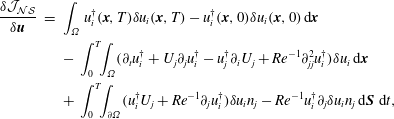 $$\begin{eqnarray}\displaystyle \frac{\unicode[STIX]{x1D6FF}{\mathcal{J}}_{{\mathcal{N}}{\mathcal{S}}}}{\unicode[STIX]{x1D6FF}\boldsymbol{u}} & = & \displaystyle \int _{\unicode[STIX]{x1D6FA}}u_{i}^{\dagger }(\boldsymbol{x},T)\unicode[STIX]{x1D6FF}u_{i}(\boldsymbol{x},T)-u_{i}^{\dagger }(\boldsymbol{x},0)\unicode[STIX]{x1D6FF}u_{i}(\boldsymbol{x},0)\,\text{d}\boldsymbol{x}\nonumber\\ \displaystyle & & \displaystyle -\,\int _{0}^{T}\!\!\int _{\unicode[STIX]{x1D6FA}}(\unicode[STIX]{x2202}_{t}u_{i}^{\dagger }+U_{j}\unicode[STIX]{x2202}_{j}u_{i}^{\dagger }-u_{j}^{\dagger }\unicode[STIX]{x2202}_{i}U_{j}+Re^{-1}\unicode[STIX]{x2202}_{jj}^{2}u_{i}^{\dagger })\unicode[STIX]{x1D6FF}u_{i}\,\text{d}\boldsymbol{x}\nonumber\\ \displaystyle & & \displaystyle +\,\int _{0}^{T}\!\!\int _{\unicode[STIX]{x2202}\unicode[STIX]{x1D6FA}}(u_{i}^{\dagger }U_{j}+Re^{-1}\unicode[STIX]{x2202}_{j}u_{i}^{\dagger })\unicode[STIX]{x1D6FF}u_{i}n_{j}-Re^{-1}u_{i}^{\dagger }\unicode[STIX]{x2202}_{j}\unicode[STIX]{x1D6FF}u_{i}n_{j}\,\text{d}\boldsymbol{S}\,\,\text{d}t,\end{eqnarray}$$
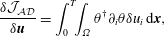 $$\begin{eqnarray}\displaystyle & \displaystyle \frac{\unicode[STIX]{x1D6FF}{\mathcal{J}}_{{\mathcal{A}}{\mathcal{D}}}}{\unicode[STIX]{x1D6FF}\boldsymbol{u}}=\int _{0}^{T}\!\!\int _{\unicode[STIX]{x1D6FA}}\unicode[STIX]{x1D703}^{\dagger }\unicode[STIX]{x2202}_{i}\unicode[STIX]{x1D703}\unicode[STIX]{x1D6FF}u_{i}\,\text{d}\boldsymbol{x}, & \displaystyle\end{eqnarray}$$
 $$\begin{eqnarray}\displaystyle & \displaystyle \frac{\unicode[STIX]{x1D6FF}{\mathcal{J}}_{{\mathcal{C}}}}{\unicode[STIX]{x1D6FF}\boldsymbol{u}}=\int _{0}^{T}\!\!\int _{\unicode[STIX]{x2202}\unicode[STIX]{x1D6FA}}p^{\dagger }\unicode[STIX]{x1D6FF}u_{i}n_{i}\,\text{d}\boldsymbol{S}\,\,\text{d}t-\int _{0}^{T}\!\!\int _{\unicode[STIX]{x1D6FA}}\unicode[STIX]{x2202}_{i}p^{\dagger }\unicode[STIX]{x1D6FF}u_{i}\,\text{d}\boldsymbol{x}, & \displaystyle\end{eqnarray}$$
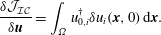 $$\begin{eqnarray}\displaystyle & \displaystyle \frac{\unicode[STIX]{x1D6FF}{\mathcal{J}}_{{\mathcal{I}}{\mathcal{C}}}}{\unicode[STIX]{x1D6FF}\boldsymbol{u}}=\int _{\unicode[STIX]{x1D6FA}}u_{0,i}^{\dagger }\unicode[STIX]{x1D6FF}u_{i}(\boldsymbol{x},0)\,\text{d}\boldsymbol{x}. & \displaystyle\end{eqnarray}$$
The requirement that
 $\unicode[STIX]{x1D6FF}{\mathcal{L}}/\unicode[STIX]{x1D6FF}\boldsymbol{u}=0$
for all
 $\unicode[STIX]{x1D6FF}\boldsymbol{u}$
thus yields the governing equation which the adjoint velocity must satisfy
 $$\begin{eqnarray}\displaystyle \unicode[STIX]{x2202}_{t}u_{i}^{\dagger }+U_{j}\unicode[STIX]{x2202}_{j}u_{i}^{\dagger }-u_{j}^{\dagger }\unicode[STIX]{x2202}_{i}U_{j}+Re^{-1}\unicode[STIX]{x2202}_{jj}u_{i}^{\dagger }+\unicode[STIX]{x2202}_{i}p^{\dagger } & =\unicode[STIX]{x1D703}^{\dagger }\unicode[STIX]{x2202}_{i}\unicode[STIX]{x1D703}-(1-\unicode[STIX]{x1D6FC})u_{i}, & \displaystyle\end{eqnarray}$$
and the initial and terminal conditions
 $$\begin{eqnarray}\displaystyle u_{0,i}^{\dagger }=u^{\dagger }(\boldsymbol{x},0),\quad u_{i}^{\dagger }(\boldsymbol{x},T)=0. & & \displaystyle\end{eqnarray}$$
Moreover, from the boundary term (i.e. the third integral in (A 9)) we obtain that
 $u_{i}^{\dagger }$
satisfies no-slip boundary conditions on the walls.
The variation
 $\unicode[STIX]{x1D6FF}{\mathcal{J}}/\unicode[STIX]{x1D6FF}\unicode[STIX]{x1D703}$
depends on the value of the switch
 $\unicode[STIX]{x1D6FD}$
. For
 $\unicode[STIX]{x1D6FD}=-1$
we obtain
 $$\begin{eqnarray}\displaystyle \frac{\unicode[STIX]{x1D6FF}{\mathcal{J}}}{\unicode[STIX]{x1D6FF}\unicode[STIX]{x1D703}}=\unicode[STIX]{x1D6FC}\int _{\unicode[STIX]{x2202}\unicode[STIX]{x1D6FA}}\unicode[STIX]{x2202}_{i}\unicode[STIX]{x1D703}\unicode[STIX]{x1D6FF}\unicode[STIX]{x1D703}n_{i}\,\text{d}\boldsymbol{S}\,\,\text{d}t-\unicode[STIX]{x1D6FC}\int _{\unicode[STIX]{x1D6FA}}\unicode[STIX]{x2202}_{ii}^{2}\unicode[STIX]{x1D703}\unicode[STIX]{x1D6FF}\unicode[STIX]{x1D703}\,\text{d}\boldsymbol{x}, & & \displaystyle\end{eqnarray}$$
while for
 $\unicode[STIX]{x1D6FD}=0$
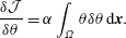 $$\begin{eqnarray}\displaystyle \frac{\unicode[STIX]{x1D6FF}{\mathcal{J}}}{\unicode[STIX]{x1D6FF}\unicode[STIX]{x1D703}}=\unicode[STIX]{x1D6FC}\int _{\unicode[STIX]{x1D6FA}}\unicode[STIX]{x1D703}\unicode[STIX]{x1D6FF}\unicode[STIX]{x1D703}\,\text{d}\boldsymbol{x}. & & \displaystyle\end{eqnarray}$$
Finally, for
 $\unicode[STIX]{x1D6FD}=1$
we obtain
 $$\begin{eqnarray}\displaystyle \frac{\unicode[STIX]{x1D6FF}{\mathcal{J}}}{\unicode[STIX]{x1D6FF}\unicode[STIX]{x1D703}} & = & \displaystyle \unicode[STIX]{x1D6FC}\int _{\unicode[STIX]{x2202}\unicode[STIX]{x1D6FA}}\unicode[STIX]{x1D6E9}\unicode[STIX]{x2202}_{i}\unicode[STIX]{x1D6E9}\unicode[STIX]{x1D6FF}n_{i}\,\text{d}\boldsymbol{S}\,\,\text{d}t-\unicode[STIX]{x1D6FC}\int _{\unicode[STIX]{x1D6FA}}\unicode[STIX]{x1D6E9}\unicode[STIX]{x2202}_{ii}^{2}\unicode[STIX]{x1D6FF}\unicode[STIX]{x1D6E9}\,\text{d}\boldsymbol{x}\end{eqnarray}$$
 $$\begin{eqnarray}\displaystyle & = & \displaystyle \unicode[STIX]{x1D6FC}\int _{\unicode[STIX]{x2202}\unicode[STIX]{x1D6FA}}\unicode[STIX]{x1D6E9}\unicode[STIX]{x2202}_{i}\unicode[STIX]{x1D6E9}\unicode[STIX]{x1D6FF}n_{i}\,\text{d}\boldsymbol{S}\,\,\text{d}t-\unicode[STIX]{x1D6FC}\int _{\unicode[STIX]{x1D6FA}}\unicode[STIX]{x2202}_{ii}^{-2}\unicode[STIX]{x1D703}\unicode[STIX]{x1D6FF}\unicode[STIX]{x1D703}\,\text{d}\boldsymbol{x}.\end{eqnarray}$$
The remaining term in the variation of
 ${\mathcal{L}}$
with respect to
 $\unicode[STIX]{x1D703}$
is
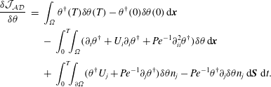 $$\begin{eqnarray}\displaystyle \begin{array}{@{}rcl@{}}\displaystyle \frac{\unicode[STIX]{x1D6FF}{\mathcal{J}}_{{\mathcal{A}}{\mathcal{D}}}}{\unicode[STIX]{x1D6FF}\unicode[STIX]{x1D703}}\ & =\ & \displaystyle \int _{\unicode[STIX]{x1D6FA}}\unicode[STIX]{x1D703}^{\dagger }(T)\unicode[STIX]{x1D6FF}\unicode[STIX]{x1D703}(T)-\unicode[STIX]{x1D703}^{\dagger }(0)\unicode[STIX]{x1D6FF}\unicode[STIX]{x1D703}(0)\,\text{d}\boldsymbol{x}\\ \ & \ & \displaystyle -\,\int _{0}^{T}\!\!\int _{\unicode[STIX]{x1D6FA}}(\unicode[STIX]{x2202}_{t}\unicode[STIX]{x1D703}^{\dagger }+U_{i}\unicode[STIX]{x2202}_{i}\unicode[STIX]{x1D703}^{\dagger }+Pe^{-1}\unicode[STIX]{x2202}_{ii}^{2}\unicode[STIX]{x1D703}^{\dagger })\unicode[STIX]{x1D6FF}\unicode[STIX]{x1D703}\,\text{d}\boldsymbol{x}\\ \ & \ & \displaystyle +\,\int _{0}^{T}\!\!\int _{\unicode[STIX]{x2202}\unicode[STIX]{x1D6FA}}(\unicode[STIX]{x1D703}^{\dagger }U_{j}+Pe^{-1}\unicode[STIX]{x2202}_{j}\unicode[STIX]{x1D703}^{\dagger })\unicode[STIX]{x1D6FF}\unicode[STIX]{x1D703}n_{j}-Pe^{-1}\unicode[STIX]{x1D703}^{\dagger }\unicode[STIX]{x2202}_{j}\unicode[STIX]{x1D6FF}\unicode[STIX]{x1D703}n_{j}\,\text{d}\boldsymbol{S}\,\,\text{d}t.\end{array} & & \displaystyle\end{eqnarray}$$
Therefore, the governing equation for the adjoint variable
 $\unicode[STIX]{x1D703}^{\dagger }$
is
 $$\begin{eqnarray}\displaystyle \unicode[STIX]{x1D703}^{\dagger }+U_{i}\unicode[STIX]{x2202}_{i}\unicode[STIX]{x1D703}^{\dagger }+Pe^{-1}\unicode[STIX]{x2202}_{ii}^{2}\unicode[STIX]{x1D703}^{\dagger }=0, & & \displaystyle\end{eqnarray}$$
with the second terminal condition
 $$\begin{eqnarray}\displaystyle \quad \unicode[STIX]{x1D703}^{\dagger }(\boldsymbol{x},T)=(-1)^{\unicode[STIX]{x1D6FD}}\unicode[STIX]{x1D6FC}\unicode[STIX]{x1D735}^{-2\unicode[STIX]{x1D6FD}}\unicode[STIX]{x1D703}(\boldsymbol{x},T), & & \displaystyle\end{eqnarray}$$
and from the boundary term (i.e. the third equation in (A 19)),
 $\unicode[STIX]{x1D703}^{\dagger }$
satisfies homogeneous Neumann boundary conditions on the walls.
Additionally, the variation with respect to the pressure,
 $$\begin{eqnarray}\displaystyle \frac{\unicode[STIX]{x1D6FF}{\mathcal{J}}_{{\mathcal{N}}{\mathcal{S}}}}{\unicode[STIX]{x1D6FF}p}=\int _{0}^{T}\!\!\int _{\unicode[STIX]{x2202}\unicode[STIX]{x1D6FA}}u_{i}^{\dagger }\unicode[STIX]{x1D6FF}pn_{i}\,\text{d}\boldsymbol{S}\,\,\text{d}t-\int _{0}^{T}\!\!\int _{\unicode[STIX]{x1D6FA}}\unicode[STIX]{x2202}_{i}u_{i}^{\dagger }\unicode[STIX]{x1D6FF}p\,\text{d}\boldsymbol{x}, & & \displaystyle\end{eqnarray}$$
yields the incompressibility condition
 $$\begin{eqnarray}\unicode[STIX]{x1D735}\boldsymbol{\cdot }\boldsymbol{u}^{\dagger }=0.\end{eqnarray}$$
Naturally (by construction) variations with respect to the adjoint variables result in the condition that the (direct) governing equations (2.17)–(2.19) are satisfied.
Finally, noting that the variation of
 ${\mathcal{L}}$
with respect to
 $\boldsymbol{u}_{0}$
is
 $$\begin{eqnarray}\displaystyle \frac{\unicode[STIX]{x1D6FF}{\mathcal{L}}}{\unicode[STIX]{x1D6FF}\boldsymbol{u}_{0}}=\frac{\unicode[STIX]{x1D6FF}{\mathcal{J}}_{{\mathcal{I}}{\mathcal{C}}}}{\unicode[STIX]{x1D6FF}\boldsymbol{u}_{0}}=\int _{0}^{T}\!\!\int _{\unicode[STIX]{x1D6FA}}u_{i}^{\dagger }\unicode[STIX]{x1D6FF}u_{0,i}\,\text{d}\boldsymbol{x}, & & \displaystyle\end{eqnarray}$$
the system of equations used by the DAL method is closed with
 $$\begin{eqnarray}\displaystyle \unicode[STIX]{x1D735}_{\boldsymbol{u}_{0}}{\mathcal{L}}=\boldsymbol{u}_{0}^{\dagger }. & & \displaystyle\end{eqnarray}$$
Appendix B. Resolution sensitivity and convergence properties of the results
The results presented in this paper arise from solutions of the constrained optimisation problem (2.26), obtained using the direct-adjoint looping (DAL) method as described briefly in § 2.3. This gradient-based minimisation method relies on numerical integration of the two systems of partial differential equations (2.17)–(2.19) and (2.32)–(2.34), which in turn relies on a discretisation of the problem in hand. The purpose of this appendix is to present supporting evidence for the choice of the resolution used herein and to provide detailed information on the convergence properties of the solutions generated by the DAL method.
The computational domain, a cuboid box
 $4\unicode[STIX]{x03C0}\times 2\times \unicode[STIX]{x03C0}$
, is discretised using
 $N_{x}=256$
uniformly distributed grid points in the streamwise direction,
 $N_{z}=64$
uniformly distributed grid points in the spanwise direction and
 $N_{y}=209$
grid points in the wall-normal direction. In order to resolve the near-wall high-shear regions, the grid points in the wall-normal direction are non-uniformly distributed according to the stretching formula (Vinokur Reference Vinokur1983)
 $$\begin{eqnarray}\displaystyle y_{j}=\tanh \left(C\left(\frac{2(j-1)}{N}-1\right)\right),\quad j=0,\ldots ,N+2, & & \displaystyle\end{eqnarray}$$
where the stretching parameter
 $C=1.75$
. The points
 $y_{j}$
form, when scaled and mapped onto the interval
 $[-1,1]$
, the vertical base grid. In addition, the fractional grid
 $$\begin{eqnarray}\displaystyle y_{j+1/2}={\textstyle \frac{1}{2}}(y_{j}+y_{j+1/2}),\quad j=0,\ldots ,N+1, & & \displaystyle\end{eqnarray}$$
is used to discretise the (
 $v$
)
 $y$
-velocity component. Here, the scaling is chosen in such a way that the fractional grid points
 $y_{3/2}$
and
 $y_{N_{y}+3/2}$
coincide with the walls (see Bewley (Reference Bewley2008) for more details).
For the considered
 $N_{y}$
, the introduced stretching function yields
 $y$
-grid size between
 $\unicode[STIX]{x0394}y_{max}=0.0185$
and
 $\unicode[STIX]{x0394}y_{min}=0.0021$
. Spatial derivatives are calculated using second-order finite differences in the wall-normal direction, and in Fourier space in the other two directions. Therefore, it is to be expected that the key resolution constraints are in the wall-normal direction. The grid resolution is uniform in both the streamwise and spanwise directions,
 $\unicode[STIX]{x03C0}/64=0.0491$
.
The resolution used in our simulations is similar to those used in various direct numerical simulation studies on turbulent channel flows (e.g. Kim, Moin & Moser Reference Kim, Moin and Moser1987; Moser, Kim & Mansour Reference Moser, Kim and Mansour1999; Tsukahara et al. Reference Tsukahara, Seki, Kawamura and Tochio2005). However, the literature focuses mostly on fully developed flows, which is not the case for the problem in hand because we largely consider inherently time-dependent transition to turbulence. The non-dimensional Kolmogorov length scale
 $$\begin{eqnarray}\displaystyle \unicode[STIX]{x1D702}=\sqrt[4]{\frac{1}{\unicode[STIX]{x1D716}\,Re^{2}}}, & & \displaystyle\end{eqnarray}$$
where
 $\unicode[STIX]{x1D716}$
denotes the non-dimensional energy dissipation rate, can be used as a rule of thumb for the necessary grid size
 $\unicode[STIX]{x1D6E5}_{min}$
, with a common assumption being that
 $\unicode[STIX]{x1D6E5}_{min}\lesssim 2\unicode[STIX]{x1D702}$
.
However, here, due to the transient nature of the studied problem,
 $\unicode[STIX]{x1D716}$
needs to be regarded as a time-dependent scalar instead of a constant. For illustration, figure 23 plots the time evolution of the energy dissipation rate for the optimal flow fields for optimisation time horizon
 $T=5$
, i.e. for the flow field visualised in figures 17, 18 and 20. It is apparent that
 $\unicode[STIX]{x1D716}$
peaks near the optimisation horizon and that the implied minimal (instantaneous) Kolmogorov length scale is smaller than the proposed grid size. For instance, the mixing strategy which is based on the mix-norm minimisation produces
 $\unicode[STIX]{x1D716}\sim 10$
, which implies
 $\unicode[STIX]{x1D702}\sim 0.0103$
. Thus, it is natural to ask whether the used resolution is sufficient, although it does appear to be satisfactory in the wall-normal direction.


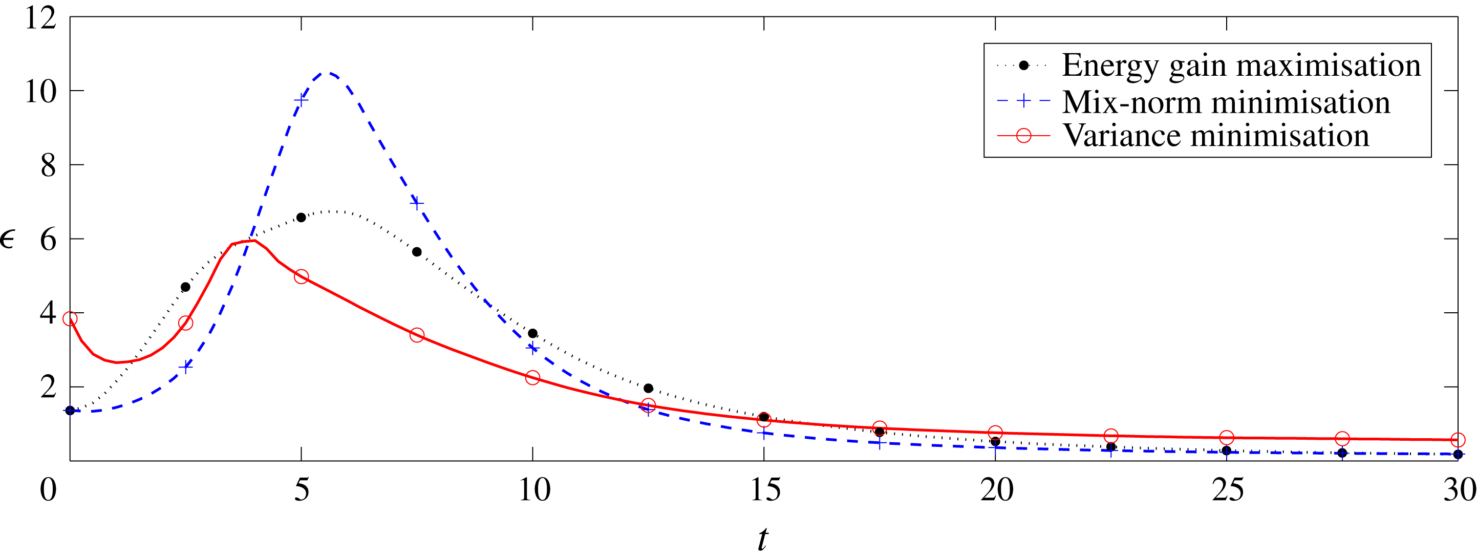
Mix-norm minimisation problem (2.26) with
 $T=2$
and
 $\unicode[STIX]{x1D6FC}=1$
,
 $\unicode[STIX]{x1D6FD}=1$
. (a) The value of the scaled mix-norm
 $M(T)$
at the target time
 $T=2$
, i.e. the optimised quantity defined in (B 4), as a function of the number of iterations. (b) The relative change of the optimised quantity
 $\unicode[STIX]{x0394}M(T)$
, as defined in (B 5), as a function of the number of iterations at the target time
 $T=2$
. (c) The scaled residual
 $r$
at the target time
 $T=2$
, as defined in (B 6), as a function of the number of iterations. (d) The time evolution of the scaled mix-norm
 $M(t)$
for the solution after 150 iterations. Different line types denote the results from the five different resolutions as listed in table 1.
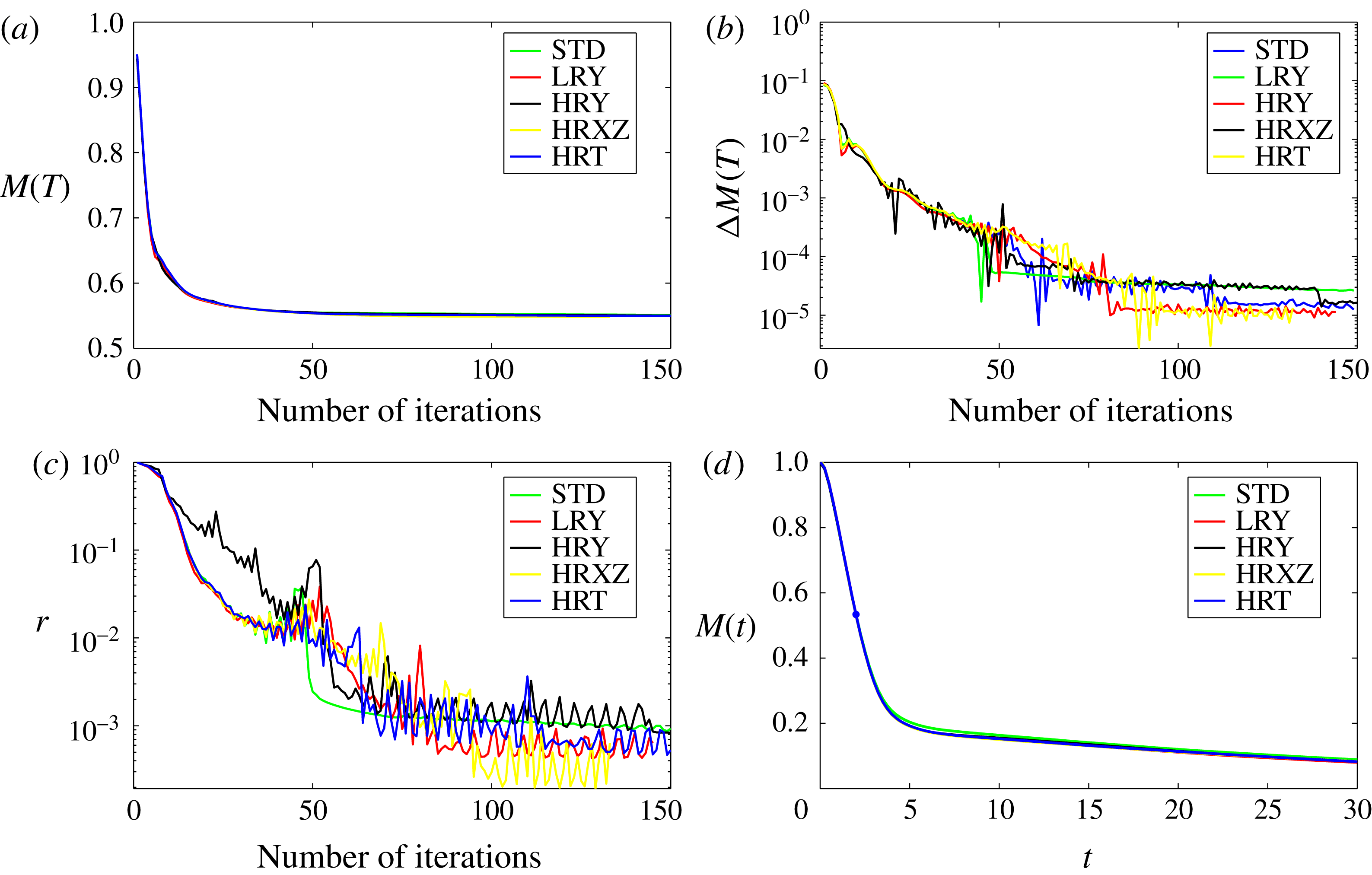
To answer this question, we carry out a series of tests to examine the sufficiency of the chosen mesh as well as the precision of results produced using the DAL method. For five different resolutions, listed in table 1, we solve the problem (2.26) with
 $\unicode[STIX]{x1D6FC}=1$
,
 $\unicode[STIX]{x1D6FD}=1$
and
 $T=2$
, i.e. we minimise the mix-norm. We choose the mix-norm minimisation solution because this particular flow produces, as illustrated in figure 23, the highest energy dissipation rate. We choose the time horizon
 $T=2$
because we observe that the shortest considered optimisation horizons give rise to the smallest vortices in the optimal flow field. Thus, we expect that mix-norm minimisation with
 $T=2$
will lead to the most challenging test of resolution.
We plot the key flow characteristics in figure 24. We consider the value of the mix-norm scaled by the diffusive process defined in (3.3), i.e.
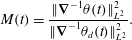 $$\begin{eqnarray}\displaystyle M(t)=\frac{\Vert \unicode[STIX]{x1D735}^{-1}\unicode[STIX]{x1D703}(t)\Vert _{L^{2}}^{2}}{\Vert \unicode[STIX]{x1D735}^{-1}\unicode[STIX]{x1D703}_{d}(t)\Vert _{L^{2}}^{2}}. & & \displaystyle\end{eqnarray}$$
Figure 24(a) shows the variation of
 $M(T)$
at the target time, i.e.
 $M(2)$
, with the number of iteration ‘loops’ of the DAL method, while figure 24(b) plots the relative change of the same value,
 $$\begin{eqnarray}\displaystyle \unicode[STIX]{x0394}M(T)=\frac{M_{n}(T)-M_{n-1}(T)}{M_{n}(T)}. & & \displaystyle\end{eqnarray}$$
We observe that
 $\unicode[STIX]{x0394}M(T)$
decreases to
 $O(10^{-5})$
for all considered resolutions, which indicates good convergence of the iterative ‘looping’ algorithm. From figure 24(a), it is apparent that the ‘standard’ resolution (labelled STD) yields
 $M(2)\approx 0.5499$
. Using the higher-resolution grids HRXZ and HRY, the DAL method yields values of
 $M(2)\approx 0.5504$
and
 $M(2)\approx 0.5496$
, respectively, corresponding to variation from the STD result of less than 0.09 %. Using higher temporal resolution (labelled HRT), the DAL method yields
 $M(2)\approx 0.5483$
, a variation of 0.29 % from the STD result. Finally, we note that the lower vertical resolution simulation (labelled LRY) also yields a good approximation,
 $M(2)=0.5514$
.
Five resolutions used to test the DAL method. The resolution labelled ‘STD’ is the one used throughout the main body of the paper.
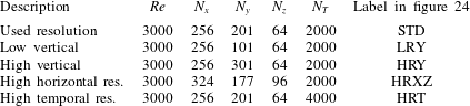
The relative change
 $\unicode[STIX]{x0394}M(T)$
approaching very small values is primarily an indication of convergence of the algorithm. To build confidence that the resulting initial flow field
 $\boldsymbol{u}_{0}$
is a minimiser of the cost functional (2.26), or at least its discrete approximation, it is necessary to examine the gradient of the cost functional with respect to
 $\boldsymbol{u}_{0}$
. Thus, following Rabin et al. (Reference Rabin, Caulfield and Kerswell2012) and Foures et al. (Reference Foures, Caulfield and Schmid2014), we consider the scaled ‘residual’
 $$\begin{eqnarray}\displaystyle r=\frac{\Vert \unicode[STIX]{x1D735}_{\boldsymbol{u}_{0}}{\mathcal{L}}^{\bot }\Vert _{L^{2}}^{2}}{\Vert \unicode[STIX]{x1D735}_{\boldsymbol{u}_{0}}{\mathcal{L}}\Vert _{L^{2}}^{2}}. & & \displaystyle\end{eqnarray}$$
The residual
 $r$
represents the norm of the projection of the gradient
 $\unicode[STIX]{x1D735}_{\boldsymbol{u}_{0}}{\mathcal{L}}$
onto the hyperplane tangent to the energy hypersurface (2.23), scaled by the norm of that gradient. For the five test grid resolutions, we plot the evolution of
 $r$
as a function of the number of iterations in figure 24(c). For each resolution,
 $r$
decays to less than
 $10^{-3}$
before apparently asymptoting to a non-zero value. Unsurprisingly, this asymptotic value decreases with increasing resolution, and in particular it appears to depend upon the wall-normal and temporal resolutions. For all resolutions, the asymptotic value is far larger than machine precision and so our results should only be regarded as approximations.
The fact that the residual does not approach zero is a consequence of the finite precision of the solutions to the partial differential equations (2.17)–(2.19) and (2.32)–(2.34). In each iteration of the DAL method, which involves integration of both the direct and adjoint equations, the gradient of the cost functional
 $\unicode[STIX]{x1D735}_{\boldsymbol{u}_{0}}{\mathcal{L}}$
is computed. This gradient inevitably has limited precision due to both the discretisation and the integration scheme itself. This error then propagates through the conjugate-gradient method used for updating the initial flow field at the beginning of each iteration. As the iterations progress and the algorithm approaches an extremal value of the cost functional, the precision of the gradient becomes progressively more important. Eventually, the method reaches a point when a better approximation cannot be reached without a better approximation of the gradient. However, we believe that the associated initial perturbation is ‘close’ to the desired initial perturbation associated with the true extremal value of the cost functional.
It is natural to assume that any error introduced via optimisation (to the target horizon
 $T$
) is further propagated when the flow is integrated for times
 $t\gg T$
. Figure 24(d) shows time evolutions of
 $M(t)$
for flows which start from the optimal initial conditions obtained using the five different test grids as introduced in table 1 after 150 iterations of the DAL method. As is apparent from the figure, the evolutions of the various simulations at different resolutions are initially indistinguishable. However, when the flow enters the third and final ‘diffusive’ stage, as discussed in § 3.2, which corresponds to the final flatter part of the lines shown in figure 24(d), the various flow evolutions start to separate slightly.
This separation is evident in figure 24 for times
 $t\gtrsim 5$
. In particular, the scaled values of the mix-norm
 $M(30)$
computed using the grids with higher spatial resolution, HRY and HRXZ, differ from the one produced with the standard ‘STD’ grid resolution by approximately 2.9 % and 0.8 %, respectively, while the relative difference between
 $M(30)$
calculated in the higher time resolution HRT simulation and
 $M(30)$
calculated in the STD simulation is approximately 0.9 %. Such differences strongly suggest that the STD grid does not fully resolve the very smallest scales where diffusive effects occur. In particular, during the final diffusion-dominated stage of mixing, higher resolution apparently marginally increases the effectiveness of mixing, which results in a fractionally faster decay of
 $M(t)$
. Nevertheless, this (perhaps unsurprising) effect is small, and does not modify the central fluid dynamical observations we have made concerning the initial structure of the various ‘optimal’ perturbations, and the subsequent leading-order flow dynamics.
Taken all together, this resolution sensitivity analysis demonstrates that the numerical precision of our results is indeed bounded. Nevertheless, it is important to appreciate that the task in hand, with
 ${\sim}10^{7}$
variables to optimise, can be regarded as a large-scale optimisation problem (Benson, Shanno & Vanderbei Reference Benson, Shanno and Vanderbei2003) and the criterion
 $r\rightarrow 0$
with
 $r$
defined in (B 6) represents a relatively strong condition (Foures et al.
Reference Foures, Caulfield and Schmid2013). The primary objective here is to compare and contrast mixing strategies which are based on different physical phenomena, and for this objective it appears that the chosen resolution is more than sufficient. Hence, although the simulations are marginally under-resolved near short-time optimisation horizons, we are confident that the central conclusions drawn from the various computed integral quantities are robust.