2 Equilibrium cylindrical model of the geomagnetic tail

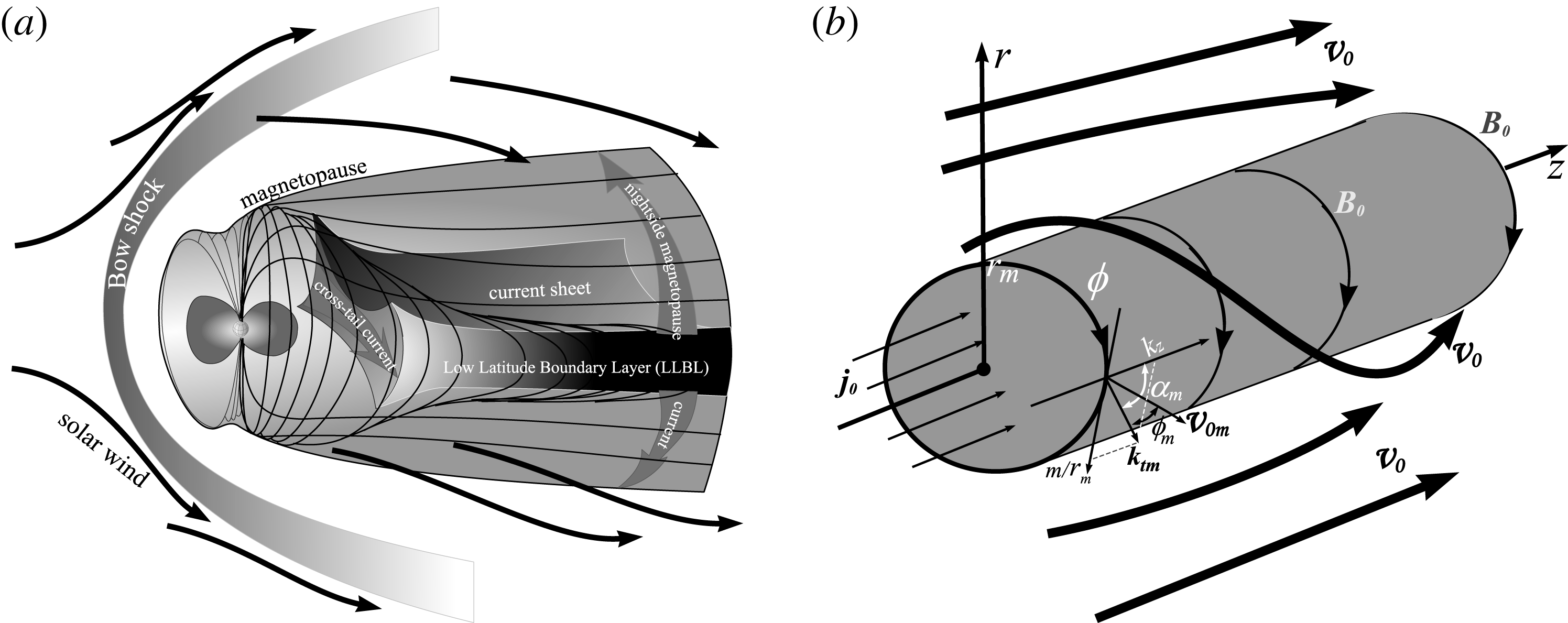
The low-latitude boundary layer of the geotail is a region of the magnetopause within $\pm (3\div 5)~R_{E}$ (where $R_{E}$ is the Earth’s radius) from the equatorial surface (see figure 1 a). Its features in the geotail include the spreading out of the cross-tail current on the magnetopause and the magnetic field lines being almost perpendicular to the solar wind flow. To describe the LLBL instability we use a cylindrical model of the geotail with a longitudinal current (see figure 1 b). This current creates a magnetic field having only an azimuthal component $\boldsymbol{B}_{\mathbf{0}}=(0,B_{0},0)$ in the cylindrical coordinate system $(r,\unicode[STIX]{x1D719},z)$ .

Figure 1.

The low-latitude boundary layer (LLBL): (a) schematic representation of the magnetic field lines and the electric current configuration in the geotail LLBL, (b) a cylindrical model of the geotail wrapped by a helical plasma flow.

The plasma cylinder model with a longitudinal current has been chosen for studying the geotail LLBL instability for the following reasons. We wished to take into account several LLBL features, while remaining within the framework of a balanced one-dimensional inhomogeneous model. The region confined by the shear layer has a finite cross-section in this model. This allows us to consider not only surface waves and waves escaping from the shear layer to infinity, but also the MHD oscillation eigenmodes localized inside the plasma cylinder. Such oscillations may be present in a real geomagnetic tail. Moreover, the longitudinal current inside the plasma cylinder creates a magnetic field featuring a similar shape and direction of its field lines to those in the real LLBL. The LLBL field lines have a positive curvature and their direction is normal to the solar wind flow far from the magnetosphere.

A simplified concept is generally used of the LLBL being wrapped around by the longitudinal (along the Sun–Earth direction) solar wind flow. It is evident, however, that both due to asymmetry in the geotail and curling of the solar wind flow wrapping around the magnetosphere, the shear flow velocity in the LLBL has not only a longitudinal component but also an azimuthal component. The azimuthal velocity component appears not only due to curling solar wind flow but due to oscillations of the geotail itself (geotail flapping) to a greater extent. Therefore, we assume in this paper that the wrapping plasma flow near the geotail has the form of an elongated helix (see figure 1).

Another feature of the LLBL, in contrast to the magnetopause in the geotail lobes, is that it separates two regions with a hot plasma: the magnetospheric current sheet and the solar wind. A typical concentration of plasma in the current sheet is $1\div 3~\text{cm}^{-3}$ , and in the solar wind $3\div 10~\text{cm}^{-3}$ (see Eastman & Hones Reference Eastman and Hones1979; Wang et al. Reference Wang, Lyons, Weygand, Nagai and McEntire2006). Such a small difference between them is an exception rather than the rule in the magnetosphere–solar wind system. With this in mind, we assume the plasma density to be constant in further calculations, for the sake of simplicity: $\unicode[STIX]{x1D70C}_{0}=\text{const}.$ , where the subscript 0 denotes the parameters of an undisturbed medium. We also assume that both the background plasma temperature and velocity, as well as the magnetic field, are inhomogeneous in the radial direction only. We are aware of the restrictions of the model we use, but it allows us to consider the above-mentioned features of the real magnetosphere, which would not have been possible in the earlier-used models employing Cartesian geometry.

For such a model the system of ideal MHD equations has the form

where $\text{d}/\text{d}t=\unicode[STIX]{x2202}/\unicode[STIX]{x2202}t+(\bar{\boldsymbol{v}}\boldsymbol{\cdot }\unicode[STIX]{x1D735})$ is the Lagrange derivative, $\bar{\boldsymbol{j}}$ , $\bar{\boldsymbol{B}}$ and $\bar{\boldsymbol{v}}$ are the current, magnetic field and plasma velocity vectors, $\bar{P}$ and $\bar{\unicode[STIX]{x1D70C}}$ are the plasma pressure and density, $\unicode[STIX]{x1D6FE}$ is the adiabatic index. For an undisturbed plasma in our model we have $\boldsymbol{j}_{\mathbf{0}}=(0,0,j_{0z})$ , $\boldsymbol{B}_{\mathbf{0}}=(0,B_{0},0)$ , $\boldsymbol{v}_{\mathbf{0}}=(0,v_{0\unicode[STIX]{x1D719}},v_{0z})$ . If the angle velocity of the plasma $\unicode[STIX]{x1D6FA}(r)$ is introduced, then $v_{0\unicode[STIX]{x1D719}}=r\,\unicode[STIX]{x1D6FA}$ .

Consider a homogeneous longitudinal current in the plasma cylinder

where $\bar{j}_{0}=\text{const}.$ , and $\unicode[STIX]{x1D703}(x)$ is the step function ( $\unicode[STIX]{x1D703}=0$ for $x<0$ , $\unicode[STIX]{x1D703}=1$ for $x\geqslant 0$ ), $r_{m}$ is the magnetopause radius. Hereafter, the subscript $m$ denotes the characteristic value of the relevant parameters at the magnetopause (where $r=r_{m}$ ).

Let us define the equilibrium plasma and magnetic field distributions in the model. Assume all the partial time derivatives in (2.1)–(2.4) to be zero ( $\unicode[STIX]{x2202}/\unicode[STIX]{x2202}t=0$ ). From the $z$ component of the vector equation (2.5) we have

whence

where $B_{0}\equiv |\boldsymbol{B}_{\mathbf{0}}|$ . By setting the density $\unicode[STIX]{x1D70C}_{0}$ we can determine the radial distribution of the Alfvén speed

where

and $v_{Am}=(\bar{j}_{0}r_{m}/c)\sqrt{\unicode[STIX]{x03C0}/\unicode[STIX]{x1D70C}_{0}}$ is the Alfvén speed at the magnetopause.

For obtaining the radial distribution of plasma pressure we use the $r$ component of the vector equation (2.1). The two other equations are identically zero. Given $(\boldsymbol{v}_{\mathbf{0}}\unicode[STIX]{x1D735})\boldsymbol{v}_{\mathbf{0}}=(-r\unicode[STIX]{x1D6FA}^{2},0,0)$ , we obtain the following balance equation

Integrating (2.11) over $r$ to $\infty$ , we get

For the plasma angle velocity we choose the following model

where $\bar{r}$ is the typical thickness of the magnetosheath and $\bar{\unicode[STIX]{x1D6FA}}$ is a characteristic angle velocity for the plasma flow in the magnetosheath. Let us obtain $\bar{\unicode[STIX]{x1D6FA}}$ as follows. We will define the flow helicity index at the magnetopause as $S_{m}=v_{0\unicode[STIX]{x1D719},m}/v_{0z}=\tan (\unicode[STIX]{x1D6FC}_{m}-\unicode[STIX]{x1D719}_{m})$ (see figure 1 b). Hereafter, we will assume the $v_{0z}$ component to be homogeneous in the solar wind. Then, given $v_{0\unicode[STIX]{x1D719},m}=r_{m}\unicode[STIX]{x1D6FA}(r_{m})$ , we have $\bar{\unicode[STIX]{x1D6FA}}=S_{m}v_{0z}\sqrt{1+(r_{m}/\bar{r})^{4}}/r_{m}$ .

Substituting the model expressions (2.8) and (2.13) in (2.12) we obtain the following expression for the background plasma pressure distribution

where the relation between the plasma pressure at infinity and at the magnetopause is

Now we can find the radial distribution of the plasma sound speed

where

$v_{sm}=\sqrt{\unicode[STIX]{x1D6FE}P_{0m}/\unicode[STIX]{x1D70C}_{0}}$ is the sound speed at the magnetopause, and $\unicode[STIX]{x1D6FD}_{\ast m}=v_{sm}^{2}/v_{Am}^{2}$ is a dimensionless value characterizing the gas-kinetic plasma pressure to the magnetic pressure ratio at the magnetopause. This value coincides with the plasma parameter $\unicode[STIX]{x1D6FD}_{m}=8\unicode[STIX]{x03C0}P_{0m}/B_{0m}^{2}$ with an accuracy of a factor of $\unicode[STIX]{x1D6FE}/2\approx 1$ .

Figure 2.

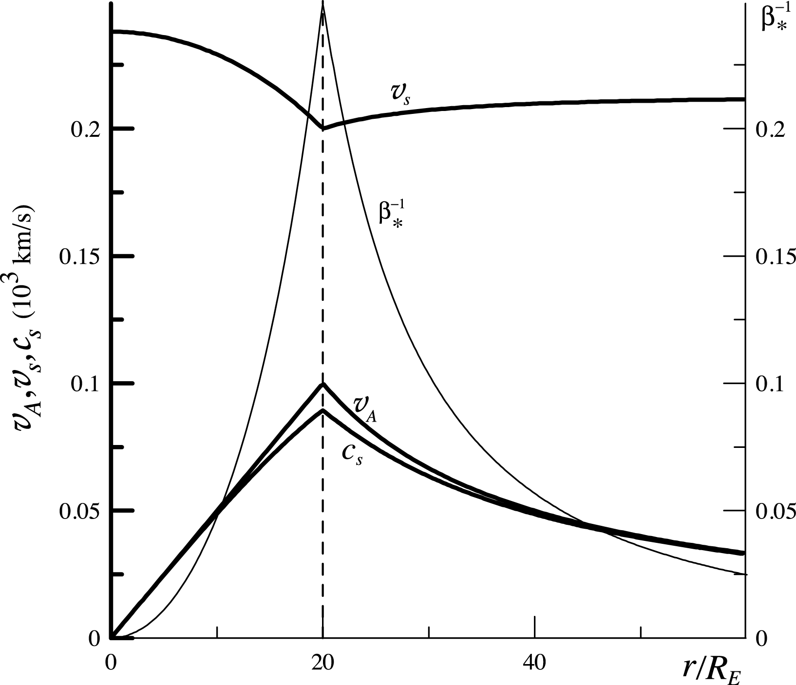
Radial distribution of Alfvén speed ( $v_{A}$ ), sound speed ( $v_{s}$ ), slow magnetosonic (SMS) speed ( $c_{s}$ ) and the $\unicode[STIX]{x1D6FD}_{\ast }^{-1}$ parameter in the geotail model for $v_{0z}=400~\text{km}~\text{s}^{-1}$ and $S_{m}=0.2$ .

To describe the distribution of the medium parameters in the geotail LLBL, the following constant values were used in further numerical calculations: $r_{m}=20R_{E}$ (where $R_{E}=6370$  km is the Earth’s radius); $\bar{r}=5R_{E}$ ; $v_{Am}=100~\text{km}~\text{s}^{-1}$ ; $v_{sm}=200~\text{km}~\text{s}^{-1}$ . The flow velocity $v_{0z}$ ranged $200$ – $1000~\text{km}~\text{s}^{-1}$ , and the flow helical index $S_{m}$ , 0 to 1. Figure 2 shows the radial distribution in the model medium (with $v_{0z}=400~\text{km}~\text{s}^{-1}$ and $S_{m}=0.2$ ) of: the Alfvén speed ( $v_{A}$ ), the sound speed ( $v_{s}$ ), the SMS wave speed ( $c_{s}$ ) and the $\unicode[STIX]{x1D6FD}_{\ast }^{-1}$ parameter, which are used in numerical calculations below. Note that the Alfvén speed, SMS wave speed and the $\unicode[STIX]{x1D6FD}_{\ast }^{-1}$ parameter distribution maxima are achieved at the magnetopause, while the maximum in the distribution of the sound speed occurs at the plasma cylinder axis. A similar behaviour of the medium parameters takes place in the real geotail LLBL region.

3 Basic equations for MHD oscillations in a cylindrical model of the magnetotail

Let us linearize the system of equations (2.1)–(2.4) with respect to small disturbances, setting $\bar{\boldsymbol{B}}=\boldsymbol{B}_{\mathbf{0}}+\boldsymbol{B}$ , $\bar{\boldsymbol{v}}=\boldsymbol{v}_{\mathbf{0}}+\boldsymbol{v}$ , $\bar{P}=P_{0}+P$ and $\bar{\unicode[STIX]{x1D70C}}=\unicode[STIX]{x1D70C}_{0}+\unicode[STIX]{x1D70C}$ , where the second term in each expression refers to disturbances associated with MHD oscillations. Then the system of linearized equations for small disturbances is of the form

It is taken into account here that $\unicode[STIX]{x1D70C}_{0}=\text{const}.$ and $\unicode[STIX]{x1D735}\boldsymbol{\cdot }\boldsymbol{v}_{\mathbf{0}}=0$ in our model. Since the equilibrium quantities are independent of $\unicode[STIX]{x1D719}$ and $z$ we will seek the solutions of (3.1)–(3.4) as an expansion in harmonics, of the form $\exp (-\text{i}\unicode[STIX]{x1D714}t+\text{i}m\unicode[STIX]{x1D719}+\text{i}k_{z}z)$ , where $\unicode[STIX]{x1D714}$ is the oscillation frequency (complex, in the general case), $m=\pm 0,1,2,\ldots$ and $k_{z}$ are the wavenumbers in the corresponding coordinates. The components of the MHD oscillation wave field can be expressed in terms of the velocity radial component $v_{r}$ as follows (see the appendix A):

where $\bar{\unicode[STIX]{x1D714}}=\unicode[STIX]{x1D714}-m\unicode[STIX]{x1D6FA}-k_{z}v_{0z}$ is the Doppler-shifted oscillation frequency in a moving medium, the prime denotes a derivative with respect to $r$ (e.g. $\unicode[STIX]{x1D6FA}^{\prime }=\text{d}\unicode[STIX]{x1D6FA}/\text{d}r$ ), and the following notations are used:

Here, the coefficients (3.11)–(3.14) have the dimension of frequency squared, $k_{t}$ is a tangential wavenumber, $\unicode[STIX]{x1D705}_{r}$ is the $r$ component of the wave vector in the Wentzel–Kramers–Brillouin (WKB) approximation as $r\rightarrow \infty$ (when the components of the wave field can be represented as ${\sim}\exp (\text{i}\int \unicode[STIX]{x1D705}_{r}\,\text{d}r)$ ), and $\unicode[STIX]{x1D718}_{s}$ is a dimensionless parameter.

If the radial component of the oscillation velocity is expressed in terms of $\unicode[STIX]{x1D701}=\text{i}v_{r}/\bar{\unicode[STIX]{x1D714}}$ (the $\unicode[STIX]{x1D701}$ parameter coincides with the plasma radial displacement in the wave when $\unicode[STIX]{x1D6FA}=0$ : $v_{r}=\text{d}\unicode[STIX]{x1D701}/\text{d}t$ ), then the equation of linear oscillations resulting from the system of equations (3.1)–(3.4) has the form

where

If the azimuthal velocity of the flow around the plasma cylinder is zero ( $\unicode[STIX]{x1D6FA}=0$ ), then we have $\tilde{\unicode[STIX]{x1D6FA}}^{2}=0$ as $r\rightarrow \infty$ , and (3.17) transforms into a well-known equation for plane-stratified flows (see Walker Reference Walker1981; Leonovich & Mishin Reference Leonovich and Mishin2005).

Let us find the solution of (3.17) in the WKB approximation. This approximation is valid for oscillations with much smaller wavelengths than the characteristic scale of the background plasma and magnetic field inhomogeneity. They are the azimuthal harmonics with $m\gg 1$ in our case. As shown by numerical calculations, however, this approximation is also fairly good at describing qualitatively (accuracy of up to 10–20 % of its eigenvalue) the basic modes ( $m=0,1,2$ ) for oscillations with wavelengths comparable to the scale of the magnetospheric plasma inhomogeneity. Let the function $\unicode[STIX]{x1D705}_{r}$ be normalized as follows: $\unicode[STIX]{x1D705}_{r}=\bar{\unicode[STIX]{x1D705}}_{r}/\unicode[STIX]{x1D716}$ (where $\unicode[STIX]{x1D716}\ll 1$ ), by extracting the large parameter $\unicode[STIX]{x1D716}^{-1}$ . We seek a solution in the form

where $\unicode[STIX]{x1D6E9}$ is a large quasi-classical phase, which we decompose as

Substituting (3.19) in (3.17) we obtain the following equation for the phase

Hence, in the zeroth order of perturbation theory, we have

where

is the square of the wavenumber in the WKB approximation. In the first order of perturbation theory we have

Thus, the solution of (3.17), in the first two orders of perturbation theory, has the form

where $C$ is an arbitrary constant,

is a pre-exponent describing the slow variation in the oscillation amplitude across magnetic shells.

To determine the form of the solution, it is necessary to set the boundary conditions for $r\rightarrow 0$ and $r\rightarrow \infty$ . In both cases, a natural requirement is that the oscillation amplitude be finite. When $r\rightarrow 0$ , the solutions are different for symmetric ( $m=0$ ) and asymmetric ( $m\neq 0$ ) modes. For symmetric modes the equation (3.17) in this case can be written as

where $\unicode[STIX]{x1D705}_{r0}=\unicode[STIX]{x1D705}_{r}(r\rightarrow 0)$ is a constant. Its solution which is finite as $r\rightarrow 0$ is

where $C_{0}$ is an arbitrary constant, $\text{J}_{1}(x)$ is the Bessel function. If the region adjacent to the plasma cylinder axis is transparent for the waves in question ( $\text{Re}\,k_{r0}^{2}>0$ ), then its asymptotic is

in the region $r\gg \unicode[STIX]{x1D705}_{r0}^{-1}$ , where $\text{J}_{1}(\unicode[STIX]{x1D705}_{r0}r)$ is matched with the WKB solution (3.25), and the WKB solution can be represented as

where $r_{t}$ is a turning point for the oscillations in question ( $r_{t}=0$ in the case at hand), and

is the total integral phase from the turning point in the geotail ( $r=r_{t}$ ) to the magnetopause ( $r=r_{m}$ ). If $\text{Re}\,\unicode[STIX]{x1D705}_{r0}^{2}<0$ and $\text{Re}\,\unicode[STIX]{x1D705}_{rm}^{2}>0$ , then there is an opacity region near the plasma cylinder axis and a turning point (where $\text{Re}\,\unicode[STIX]{x1D705}_{r}^{2}(r_{t})=0$ ) somewhere between $r=0$ and $r=r_{m}$ , which should be selected as $r_{t}$ .

Figure 3.

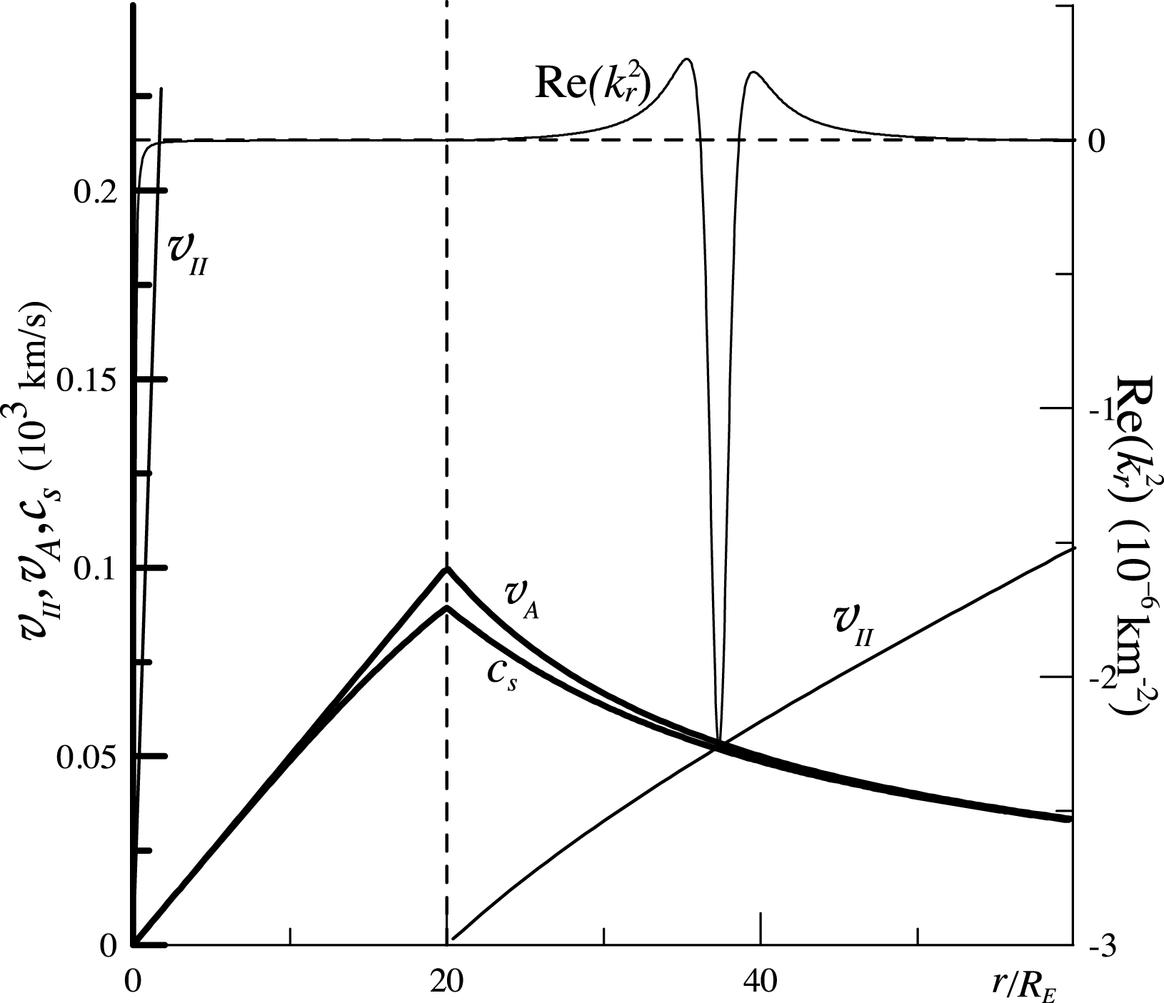
Radial distribution of the square of the wavenumber $\text{Re}\,k_{r}^{2}(r)$ for asymmetric modes of MHD oscillations (right vertical axis) and of Alfvén speed $v_{A}$ , SMS wave speed $c_{s}$ and the longitudinal phase velocity of FMS waves $v_{\Vert }=r\bar{\unicode[STIX]{x1D714}}/m$ for the harmonic with $m=1$ , $k_{z}=2\unicode[STIX]{x03C0}/10R_{E}$ (left vertical axis).

The typical behaviour of $\text{Re}\,k_{r}^{2}(r)$ for asymmetric modes ( $m\neq 0$ ) is shown in figure 3. There is an opacity region for these waves near the plasma cylinder axis (see (3.15)). If the magnetospheric near-magnetopause region is transparent for these waves ( $\text{Re}\,k_{r}^{2}(r_{m})>0$ ), the WKB solution describing the oscillation field in the magnetosphere has the same form (3.30). If this region is opaque ( $\text{Re}\,k_{r}^{2}(r_{m})<0$ ), then – for both symmetric and asymmetric modes – the WKB solution has the form

where the plus sign should be selected in the exponent for oscillations in the magnetosphere ( $r<r_{m}$ ).

Either a transparency or an opacity region can adjoin the magnetopause from the solar wind side. If an opacity region adjoins the magnetopause, the WKB solution has the same form (3.32), where the minus sign should be selected in the exponent. But if the magnetopause is adjoined by a transparency region, several options are possible. If the transparency region extends to infinity, then the wave carrying energy away from the shear layer should be chosen as the solution:

It is this solution that makes the causality principle hold for unstable oscillations originating from the shear layer (see Leonovich & Mishin Reference Leonovich and Mishin2005).

As is evident from figure 3, however, there are cases when resonance surfaces for Alfvén waves (where $v_{\Vert }=\text{Re}\,\bar{\unicode[STIX]{x1D714}}/k_{\Vert }=v_{A}$ , $k_{\Vert }$ and $v_{\Vert }$ are the wave vector and phase velocity components along the background magnetic field) and for slow magnetosonic waves (where $v_{\Vert }=c_{s}$ ) exist in the solar wind. These surfaces are defined by singular turning points separating the transparency and opacity regions for the MHD waves we are inspecting. It would seem that in this case a waveguide should also exist for waves localized between the magnetopause and the nearest turning point. However, the singular turning point separating the transparency region from the infinitely extending opacity region is special in that the total energy of the incident MHD wave is completely absorbed in its neighbourhood (see Leonovich & Mazur Reference Leonovich and Mazur1993; Leonovich & Kozlov Reference Leonovich and Kozlov2009).

In the case we examine the opacity region has a finite size, of course. Assuming that the WKB approximation is applicable, however, we have to expect its size to be much larger than the wavelength of the MHD oscillations in question. Therefore, almost the entire energy of the incident wave is absorbed near the turning point, so that a reflected wave is absent. In this case, the solution of (3.17) will also have the form of a wave radiated by the shear layer (3.33).

The dispersion equation is obtained by matching the solutions describing the MHD waves in the magnetosphere and in the solar wind. The matching conditions are determined from (3.17). If we integrate it twice across the magnetopause over a small interval $r_{m}-\unicode[STIX]{x1D716}\leqslant r\leqslant r_{m}+\unicode[STIX]{x1D716}$ , letting $\unicode[STIX]{x1D716}$ tend to zero, we obtain the first matching condition:

where the subscripts $_{+}$ and $_{-}$ mean that the values are taken from the different sides of the boundary $r=r_{m}$ : respectively from the solar wind and the magnetosphere. Condition (3.34) is called the kinematic boundary condition. If we perform a single integration of (3.17) in the same way, we obtain the second matching condition in the main order of the WKB approximation

The dispersion equation is obtained if we divide the left- and right-hand sides of (3.35) by $\unicode[STIX]{x1D701}_{+}$ and $\unicode[STIX]{x1D701}_{-}$ respectively, resulting in derivatives in (3.35) replaced with the logarithmic derivatives. The dispersion equation is more convenient to study in dimensionless variables

Here $c$ is the dimensionless phase velocity of the wave, and $M$ is the Mach number, both defined by the projection of the velocity $\boldsymbol{v}_{0m}$ onto the $\boldsymbol{k}_{tm}$ direction (see figure 1 b). Substituting dimensionless parameters in the dispersion equation lets us rewrite it as

where $\unicode[STIX]{x1D6FC}_{m}$ is the angle between the tangential wave vector at the magnetopause and the $z$ axis (see figure 1 b),

Here $\unicode[STIX]{x1D6F9}_{m}=\bar{\unicode[STIX]{x1D6F9}}+\unicode[STIX]{x03C0}/4$ . The top line in this expression corresponds to the surface wave when both sides of the shear layer are opacity regions for FMS waves. The three other lines describe various combinations in which the magnetopause adjoins the transparency regions on one or both sides.

4 Solving the dispersion equation in limiting cases

Consider a few limiting cases when the solution of the dispersion equation (3.37) can be obtained and investigated in an analytical form. For obtaining well-known limiting cases, we will consider the plasma flow around the plasma cylinder along the $z$ axis. In other words, we consider the flow with $\unicode[STIX]{x1D6FA}=0$ . In addition, let us consider the limit $k_{t}r_{m}\gg 1$ so as to proceed to a plane-stratified flow. In this limit, we have $\tilde{\unicode[STIX]{x1D6FA}}^{2}=0$ and

Consider the symmetric oscillation mode: $m=0$ . In this case, $\sin \unicode[STIX]{x1D6FC}_{m}=0$ , $\cos \unicode[STIX]{x1D719}_{m}=1$ ( $\unicode[STIX]{x1D719}_{m}$ is the angle between the vectors $\boldsymbol{v}_{0m}$ and $\boldsymbol{k}_{tm}$ ). If an opaque magnetospheric region adjoins the magnetopause, the dispersion equation (3.37) can be written as

where $\overline{M}=M\sqrt{\unicode[STIX]{x1D6FD}_{\ast m}/(1+\unicode[STIX]{x1D6FD}_{\ast m})}$ . If we use a new variable, $c^{\prime }=c-1/2$ , then it follows from this dispersion equation that

whence

One of these solutions (if the minus sign is chosen for the radical) describes unstable oscillations (with $c^{\prime 2}<0$ ), when the Mach number $\overline{M}$ is in the range

This condition corresponds completely to the one obtained previously for oscillations with $\boldsymbol{k}_{t}\bot \boldsymbol{B}_{0}$ in plane-stratified MHD flows (where $\boldsymbol{k}_{t}$ is the wave vector tangent to the shift layer, see Leonovich & Mishin Reference Leonovich and Mishin2005), as well as for ordinary hydrodynamical shear flows (Syrovatsky Reference Syrovatsky1954). Thus, there is an upper threshold on the Mach number for oscillations with $\boldsymbol{k}_{t}\bot \boldsymbol{B}_{0}$ above which the shear flow-generated oscillations become stable. However, there is no lower threshold: unstable oscillations are generated by arbitrarily slow shear flows.

The other limiting case corresponds to asymmetric oscillation modes with $m\neq 0$ for $k_{z}^{2}r_{m}^{2}\ll m^{2}$ excited by a flow with $\unicode[STIX]{x1D6FA}=0$ . In this case, $\sin \unicode[STIX]{x1D6FC}_{m}=1$ , $\cos \unicode[STIX]{x1D719}_{m}\ll 1$ . Note that for oscillations with $m=0$ we cannot simply put $k_{z}=0$ , because in this case we have $M=0$ , $|c|=\infty$ . However, the limiting transition $k_{z}\rightarrow 0$ is possible, because the variable $c$ in the dispersion equation (3.37) is multiplied by $M$ everywhere, and $k_{z}$ is cancelled out in this product. Consider the dispersion equation of the oscillation for which the magnetospheric region adjacent to the magnetopause is opaque. Proceeding to the $c^{\prime }=c-1/2$ variable in this equation, we obtain

The solution of this equation,

describes unstable oscillations (for $\unicode[STIX]{x1D6FD}_{\ast m}>1$ ), when the minus sign is chosen for the radical and the Mach number $M$ is in the range

This condition corresponds to the one obtained for oscillations with $\boldsymbol{k}_{t}\Vert \boldsymbol{B}_{0}$ in plane-stratified MHD flows (Sen Reference Sen1964; McKenzie Reference McKenzie1970a ; Leonovich & Mishin Reference Leonovich and Mishin2005). This shows that both the upper and lower thresholds exist for the Mach number interval for oscillations with $\boldsymbol{k}_{t}\Vert \boldsymbol{B}_{0}$ within which shear flow-generated oscillations are unstable. For an incompressible medium ( $\unicode[STIX]{x1D737}_{\ast }\rightarrow \infty$ ), the ranges (4.5) and (4.8) coincide, and the flow becomes hydrodynamic.

Figure 4.

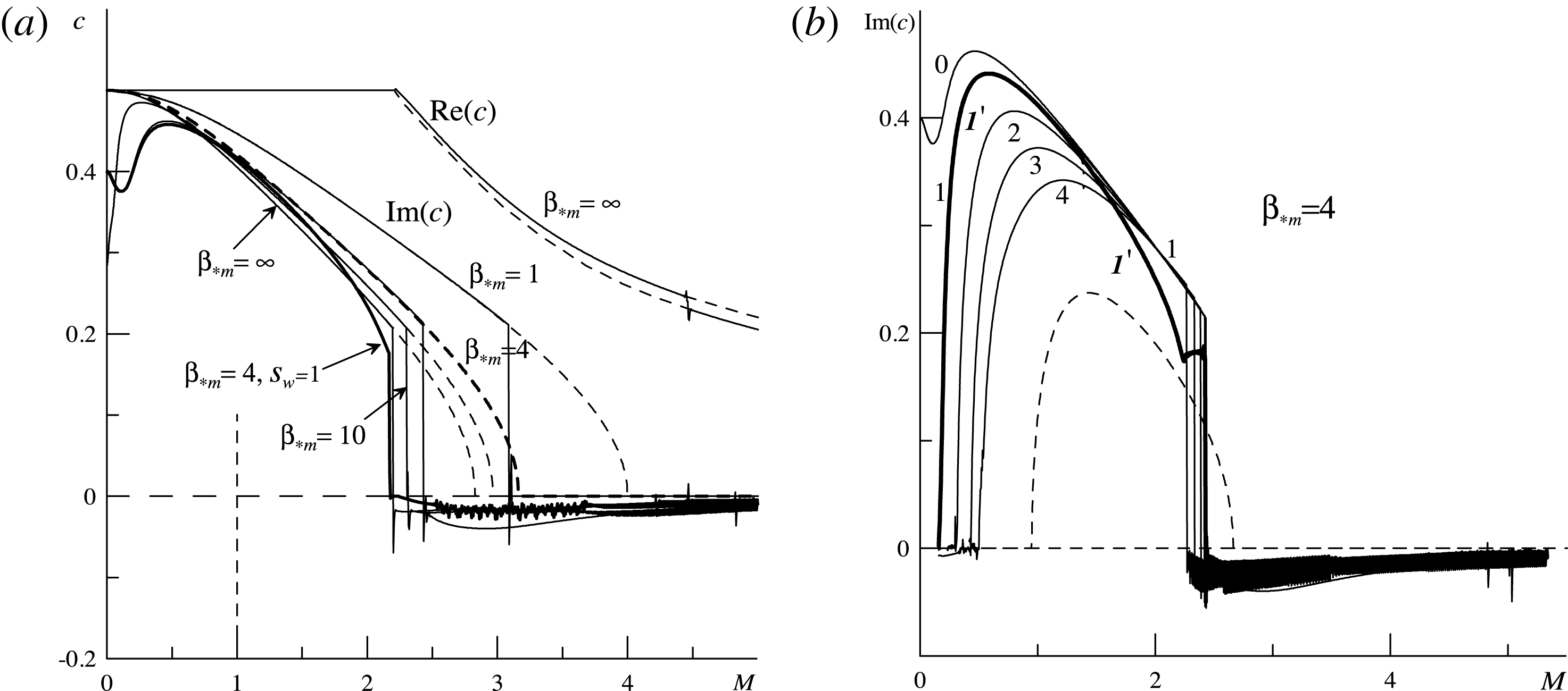
Numerical solution of the dispersion equation (3.37). The dashed curves denote the analytical solutions (4.4) and (4.7). (a) The Mach number dependence $c(M)$ for the symmetric mode ( $m=0$ , $k_{z}=2\unicode[STIX]{x03C0}/10R_{E}$ ) for different magnitudes of parameter $\unicode[STIX]{x1D6FD}_{\ast m}=1,4,10,\infty$ and the shear flow helicity index $S_{w}=0$ (thin lines), as well as for $\unicode[STIX]{x1D6FD}_{\ast m}=4$ and $S_{w}=1$ (bold line). (b) Mach number dependence of $\text{Im}\,c$ for the modes ( $m=0,1,2,3,4$ , $k_{z}=2\unicode[STIX]{x03C0}/10R_{E}$ ) when $\unicode[STIX]{x1D6FD}_{\ast m}=4$ and $S_{w}=0.2$ (thin line), and for the mode ( $m=1$ , $k_{z}=2\unicode[STIX]{x03C0}/10R_{E}$ ) when $S_{w}=1$ (bold line).

5 Numerical solution of the dispersion equation and discussion of the results

Figure 4 presents the numerical solution of the dispersion equation for various modes of the MHD oscillations for various parameters of the model medium. Figure 4(a) shows the $c(M)$ distribution for the symmetric oscillation modes ( $m=0$ ) for various magnitudes of the $\unicode[STIX]{x1D6FD}_{\ast m}$ parameter and helicity index $S_{m}$ . The distribution of the real part ( $\text{Re}\,c$ ) is given only for the case of an incompressible medium ( $\unicode[STIX]{x1D6FD}_{\ast m}=\infty$ ). The distributions of the imaginary part ( $\text{Im}\,c$ ) are given for different magnitudes of $\unicode[STIX]{x1D6FD}_{\ast m}=1,4,10,\infty$ .

Thin solid lines show the calculated distributions for a longitudinal flow around the LLBL ( $\unicode[STIX]{x1D6FA}=0$ , $S_{m}=0$ ), and the dashed lines correspond to analytical distributions given by (4.4). The thick solid line shows the distribution of $\text{Im}\,c$ for the geotail model described in § 2, when the tail is wrapped around by a flow with $S_{m}=1$ . The higher the helicity index of the wrapping flow, the greater the difference between the calculated curves and the analytical solutions. Note that $S_{m}=1$ corresponds to a strongly curled plasma flow ( $\unicode[STIX]{x1D6FC}_{m}-\unicode[STIX]{x1D719}_{m}=\unicode[STIX]{x03C0}/4$ ).

Figure 4(a) shows that the analytical and the numerical distribution of $\text{Im}\,c(M)$ for flows with $S_{m}=0$ coincide in a significant part of the calculation region. However, when $M$ exceeds the upper threshold, unstable oscillations ( $\text{Im}\,c>0$ ) become stable ( $\text{Im}\,c<0$ ). Analysis of the solutions shows that this occurs when the surface oscillation mode transforms into the radiative mode. Recall that the opacity regions for the surface modes ( $\text{Re}\,k_{r\pm }^{2}<0$ ) are located on both sides of the shear layer. For the radiative mode, transparent regions are on one or both sides of the shear layer ( $\text{Re}\,k_{r\pm }^{2}>0$ ).

In plane-stratified flows, the upper limit is not related to the surface mode transforming into the radiative mode and is determined by the conditions (4.5) and (4.8). In such flows unstable radiative oscillation modes transform into neutrally stable modes (with $\text{Im}\,c=0$ ) when $M$ exceeds the upper threshold. In the cylindrical model of the geotail, this transformation occurs when $M=M_{c}$ ( $\text{Re}\,k_{r\pm }^{2}(M_{c})=0$ ), and the mode becomes stable ( $\text{Im}\,c<0$ ).

Consider a symmetric mode ( $m=0$ ). In the medium model with a longitudinal flow ( $S_{m}=0$ ), we have, for this mode, the following expression for the squared wavenumber in the magnetosphere

This expression describes a surface wave when $\text{Re}\,k_{r-}^{2}<0$ , yielding the condition

whence

For the model with a longitudinal flow around the plasma cylinder, the instability condition (5.3) should be used instead of the condition (4.5) obtained for the plane-stratified flows. It is easy to verify that the same condition (5.3) is obtained when analysing the transformation of the surface wave into the radiative mode in the solar wind. In this case an expression similar to (5.1) is obtained for $k_{r+}^{2}$ up to the substitution $c\rightarrow c-1$ .

It should be noted, however, that the dispersion equation (3.37) has two complex conjugate solutions. One of them describes the mode that is unstable ( $\text{Im}\,c>0$ ) for the Mach number range in (5.3), but is stable ( $\text{Im}\,c<0$ ) for $M>M_{c}$ . Conversely, the complex conjugate solution describes, for the Mach number range in (5.3), the stable mode ( $\text{Im}\,c<0$ ) which is weakly unstable ( $\text{Re}\,c\gg \text{Im}\,c>0$ ) for $M>M_{c}$ . The geotail length is infinite in the cylindrical model we examine. In the real magnetosphere, however, this length is finite. Therefore, studies of various unstable oscillations should make a distinction between absolute (at fixed spatial point) and convective (at a point moving with the solar wind flow) instabilities (Mills et al. Reference Mills, Longbottom, Wright and Ruderman2000; Wright et al. Reference Wright, Mills, Ruderman and Brevdo2000). Given the finite time interval during which the convective instability exists, as well as various MHD wave dissipation mechanisms (not addressed here (see Kozlov Reference Kozlov2010; Klimushkin, Mager & Glassmeier Reference Klimushkin, Mager and Glassmeier2012; Dmitrienko Reference Dmitrienko2013)), we can neglect the presence of weakly unstable radiative modes while investigating the Kelvin–Helmholtz instability in the LLBL. The Mach number range for which the cylindrical tangential discontinuity can be regarded as unstable is then approximately determined by the condition (5.3).

Thus, the transformation of the surface wave into the radiative mode, both in the magnetosphere and in the solar wind, occurs at the same magnitude of the upper Mach number threshold $M_{c}=\sqrt{2(1+\sqrt{2})(1+\unicode[STIX]{x1D6FD}_{\ast m}^{-1})}$ . This means that the magnetopause is unstable for symmetric modes only when $v_{0}<M_{c}v_{sm}$ . In our model magnetotail ( $\unicode[STIX]{x1D6FD}_{\ast m}=4$ , $v_{sm}=200~\text{km}~\text{s}^{-1}$ ) this restriction is of the form $v_{0}<490~\text{km}~\text{s}^{-1}$ . As is evident from figure 4(a) the magnitude of $M_{c}$ decreases for helical flows. Thus, the LLBL in the geotail is unstable to such waves only in the low- and medium-velocity solar wind flows, but becomes stable in high-velocity flows.

The distribution of the real part $\text{Re}\,c$ is shown for an incompressible medium ( $\unicode[STIX]{x1D6FD}_{\ast m}=\infty$ ) in the same figure 4(a). We have $\text{Re}\,c=0.5$ for a surface wave. When it transforms into the radiative mode (when $M>M_{c}$ ), it splits into many branches, each related to one of the plasma cylinder waveguide eigenmodes. The procedure used for a numerical search of the dispersion equation roots switches from one such branch to another when the Mach number reaches the next eigenvalue $M_{n}=\unicode[STIX]{x1D714}_{n}/v_{0z}$ (where $\unicode[STIX]{x1D714}_{n}$ is the waveguide eigenfrequency, $n=0,1,2,\ldots$ ). The behaviour of $\text{Re}\,c(M)$ is similar in models with different parameters, so we will not consider it further.

The ‘tremor’ in the curves describing the distribution of the radiative mode decrements in figure 4 is due to the above jumps from one branch to the next. An example of such a jump is shown in figure 4(a). A very narrow region appears near point $M_{1}$ where the oscillations are weakly unstable ( $\text{Im}\,c>0$ ). Their growth rate is, however, so small compared with the surface wave growth rate (4.4) that this effect can be neglected.

Now we consider the asymmetric modes. Figure 4(b) presents the distribution of $\text{Im}\,c(M)$ in the model medium in question ( $\unicode[STIX]{x1D6FD}_{\ast m}=4$ ), with the longitudinal flow ( $S_{m}=0$ ), for both symmetric ( $m=0$ , $k_{z}=2\unicode[STIX]{x03C0}/10R_{E}$ ) and asymmetric modes ( $m=1,2,3,4$ , $k_{z}=2\unicode[STIX]{x03C0}/10R_{E}$ ). An analytical solution, equation (4.7), for $S_{m}=0$ , as well as a numerical solution for $S_{m}=1$ are also shown here for the mode ( $m=1$ , $k_{z}=2\unicode[STIX]{x03C0}/10R_{E}$ ).

Note the essential difference between the analytical and numerical solutions of the dispersion equation. It can be explained by the fact that for an asymmetric mode in the cylindrical model we cannot neglect the term $\tilde{\unicode[STIX]{x1D6FA}}^{2}$ , as compared to $\unicode[STIX]{x1D6FA}_{A}^{2}$ , in the definition of $k_{r}^{2}$ . The upper threshold for the instability region for asymmetric modes, same as for symmetric modes, is associated with the surface mode transforming into the radiative mode at point $M=M_{c}$ that is defined by the condition $\text{Re}\,k_{r\pm }^{2}(M_{c})=0$ . To determine this point analytically is more difficult than doing this for the symmetric mode, therefore we will not undertake it here. The upper threshold for the main azimuthal harmonics ( $m\sim 1$ ) in our geotail model is below $500~\text{km}~\text{s}^{-1}$ . Note that, in flows with a smooth shear layer, the range of the velocity jump necessary for driving unstable waves is somewhat wider.

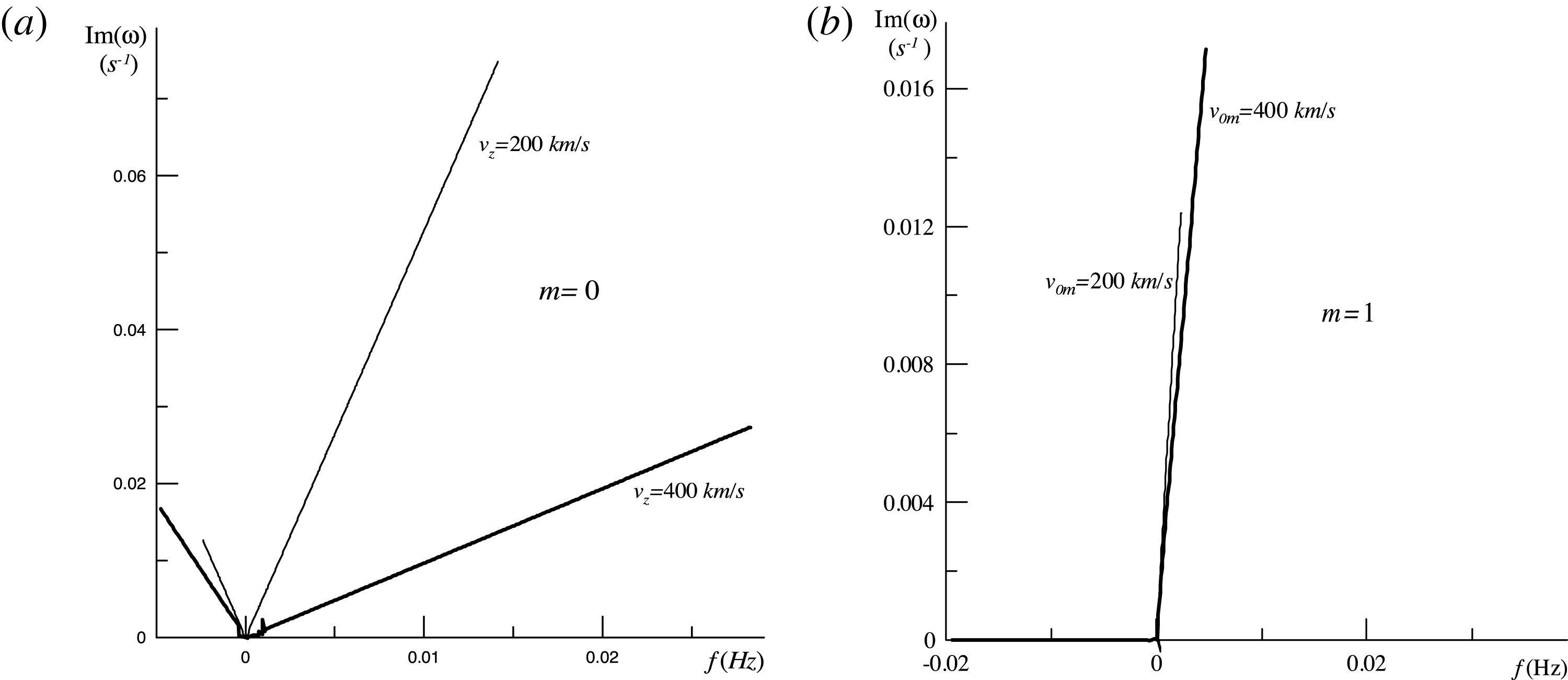
Figure 5 shows the dependences of the surface wave growth rate ( $\text{Im}(\unicode[STIX]{x1D714})$ ) on frequency ( $f=\text{Re}\,\unicode[STIX]{x1D714}/2\unicode[STIX]{x03C0}$ ). These distributions were obtained for fixed Mach number magnitudes (flow velocities $v_{0}=200,400~\text{km}~\text{s}^{-1}$ ) and the flow helicity index $S_{m}=0.2$ , when the longitudinal wave vector component varied $-10^{-3}~\text{km}^{-1}\leqslant k_{z}\leqslant 10^{-3}~\text{km}^{-1}$ . Figure 5(a) shows the distributions for the symmetric oscillation mode ( $m=0$ ), and figure 5(b), for the first harmonic ( $m=1$ ).

Figure 5.

Dependence of the surface wave growth rate in the LLBL ( $\text{Im}(\unicode[STIX]{x1D714})$ ) on frequency ( $f=\text{Re}\,\unicode[STIX]{x1D714}/2\unicode[STIX]{x03C0}$ ) for the flow helicity index $S_{m}=0.2$ and different flow velocities: $v_{0m}=200,400~\text{km}~\text{s}^{-1}$ . (a) For the symmetric mode $m=0$ . (b) For the asymmetric mode $m=1$ . The $f<0$ values correspond to $k_{z}<0$ , and the $f>0$ values to $k_{z}>0$ , respectively.

Note that the dispersion equation (3.37) for the symmetric oscillation mode remains invariant if the signs of $\unicode[STIX]{x1D714}$ and $k_{z}$ are changed simultaneously. Unstable oscillations with $f>0$ and $f<0$ in figure 5 correspond to modes with different signs of $k_{z}$ in the dispersion equation. One of them is unstable for $k_{z}>0$ , but becomes stable for $k_{z}<0$ , while the second branch is unstable for $k_{z}<0$ but stable for $k_{z}>0$ . The phase velocity signs ( $v_{ph\,z}=\unicode[STIX]{x1D714}/k_{z}$ ) are the same for these waves. In fact, they are complex conjugate solutions for the same wave.

Figure 5(b) shows a similar distribution for one of the branches of the asymmetric mode with $m=1$ . These oscillations are unstable at $f>0$ ( $k_{z}>0$ ) and become neutrally stable ( $\text{Im}\,\unicode[STIX]{x1D714}=0$ ) for $k_{z}<0$ . The linear dependence of these distributions is due to the fact that the values of $c$ are practically independent of $k_{z}$ in the range of $k_{z}$ in question.

It follows from these plots that when longitudinal wavenumber $k_{z}$ increases, both the frequency and the growth rate of the surface waves increase too. However, the analysis presented above does not take into account such an important element as the finite thickness of the shear layer. As mentioned in the introduction, the shear layer becomes stable for waves with wavelengths comparable with or smaller than its thickness. This effect requires a separate study, which we plan to do in the future.