


1 INTRODUCTION
Consider the local unit root (LUR) autoregression

with initialization
$y_0=O_P(1)$
 , innovations
$\{u_k\}_{k\ge 1}$
 , and constant localizing coefficient
$\tau \in \mathbb {R}$
 .Footnote
1
Let
$\widehat \alpha _n=\frac {\sum _{k=1}^n y_{k-1}y_k }{\sum _{k=1}^ny_{k-1}^2}$
 be the least squares (LS) estimator of
$\alpha $
 . When
$u_k \sim _{iid}(0,\sigma ^2>0)$
 it is well-known (Chan and Wei, Reference Chan and Wei1987; Phillips, Reference Phillips1987a, Reference Phillips1987b, Reference Phillips1988) that

where
$J_{\tau }=\{J_{\tau }(t)=\int _0^t e^{(t-s)\tau }dB_s\}_{t\ge 0}$
 is throughout the article a linear diffusion (Ornstein–Uhlenbeck) process satisfying
$d J_{\tau }(t) = \tau \, J_{\tau }(t)dt + dB_t,$
 with
$J_{\tau }(0)=0$
 and
$B=\{B_t\}_{t\ge 0}$
 is a standard Brownian motion.
In spite of the super consistency of (1.2) the limit distributions of
${\widehat \alpha _n}$
 and the corresponding studentized statistic are non-pivotal and depend on the unknown localizing coefficient
$\tau $
 , which is identified but not consistently estimable, as is clear from the original limit theory and much later commentary and analysis (Hansen, Reference Hansen1999; Mikusheva, Reference Mikusheva2007, Reference Mikusheva2012; Phillips, Reference Phillips2014, Reference Phillips2023). To assist in resolving this difficulty, many different approaches have been introduced in the literature. The first-difference method in Phillips and Han (Reference Phillips and Han2008) has virtually no finite sample bias, is insensitive to initial conditions, and Gaussian limit theory applies continuously as
$\alpha $
 passes through unity, but with a uniform
$\sqrt n$
 convergence rate. This rate of convergence can be improved by aggregating moment conditions in differences, as in Han, Phillips, and Sul (Reference Han, Phillips and Sul2011), leading to an estimator that has a limiting normal distribution uniformly over stationary and unit root cases with a rate of convergence within a slowly varying factor of n when
$\alpha =1$
 .
In addition to this work, several instrumental variable (IV) estimators have appeared in the literature as alternatives to standard LS. In particular, So and Shin (Reference So and Shin1999) suggested the use of the Cauchy estimator, using the sign function as an IV. Chan, Li, and Peng (Reference Chan, Li and Peng2012) generalized that approach by considering weighted estimation in model (1.1). An interesting feature of Chan, Li, and Peng (Reference Chan, Li and Peng2012) is that the studentized statistic based on the weighted LS estimator in model (1.1) has a normal limit distribution free of the parameter
$\tau $
 , enabling feasible inference concerning
$\alpha $
 . But overweighting in that approach loses the super consistency of LS estimation in LUR regression.
Time series generated according to LUR processes of the type (1.1) but with more general serially dependent innovations play a major role in the study of cointegrating and predictive regressions. Using quite a different methodology, Phillips and Magdalinos (Reference Phillips and Magdalinos2009) introduced the IVX approach which was extended in Kostakis, Magdalinos, and Stamatogiannis (Reference Kostakis, Magdalinos and Stamatogiannis2015) and designed to provide a systematic method of estimation and inference in regressions that involve near-unit-root processes. The IVX method, named for its use of instruments that are constructed endogenously, utilizes linear filtering of the regressors that mildly attenuates their signal to produce new IVs which enable IV estimation with a mixed Gaussian limit theory and a student t statistic with a standard normal limit distribution, thereby facilitating inference. For recent work on the IVX method, we refer to Magdalinos and Petrova (Reference Magdalinos and Petrova2022), Yang et al. (Reference Yang, Long, Peng and Cai2020), Demetrescu et al. (Reference Demetrescu, Georgiev, Rodrigues and Taylor2022), Shi and Phillips (Reference Shi and Phillips2022, Reference Shi and Phillips2023), and Liu and Phillips (Reference Liu and Phillips2023).
The present article proposes a new estimator that has a mixed Gaussian limit by using self-weighted (SW) estimation in (1.1). The approach can be implemented in cointegrating and predictive regressions as well as LUR regressions such as (1.1). Noting that
$y_n/\sqrt n=O_P(1)$
 in (1.1), the key idea is that the function
$I(|y_{k-1}|\le b_n \sqrt n)$
 , where
$b_n\to 0$
 , can be used as a softening weight to attenuate the signal in ordinary LS estimation theory so that Wang’s extended martingale limit theorem (Wang, Reference Wang2014; Wang, Reference Wang2015, Thm. 3.13) applies to establish the asymptotics. The idea is a subtle form of asymptotic trimming that attenuates nonstationarity in the signal sufficiently to remove nuisance parameter effects and produce mixed Gaussian limit behavior. In the context of (1.1), this article explicitly investigates the SW LS estimator
$\widehat \alpha _{1n}$
 of
$\alpha $
 defined by

for some positive numerical sequence
$b_n\to 0$
 . We show that
${\widehat \alpha }_{1n}$
 has a mixed Gaussian limit and the corresponding studentized statistic converges to a normal limit free of the parameter
$\tau $
 . This new estimator
${\widehat \alpha }_{1n}$
 retains superconsistency although the convergence rate is slightly slower than n. The reduction in the convergence rate depends on the rate at which
$b_n\to 0$
 . Indeed, noting that
$y_{\lfloor nt \rfloor }/\sqrt n \sigma \Rightarrow J_{\tau }(t)$
 on
$D[0, 1]$
 , the limit behavior of
${\widehat \alpha }_{1n}$
 , when
$b_n= b>0$
 , is similar to that of
${\widehat \alpha }_{n}$
 , so standard normal limit theory no longer applies. The sequence
$b_n \to 0$
 softens the nonstationarity in the regressor
$y_{t-1}$
 sufficiently to reduce the
$O_P(n^2)$
 signal and the associated
$O_P(n)$
 superconsistency of LS estimation but retains nonstationarity in the signal. This has the direct benefit of mixed Gaussian limit theory, independence of the localizing coefficient
$\tau $
 and standard normal asymptotics for the associated SW studentized statistic. The method therefore uses asymptotically controlled trimming of nonstationarity in the data rather than elimination of outliers as in traditional statistical methods to eliminate heavy tailed data in the estimation of a mean.
A similar truncation idea was used by Li, Tjostheim, and Gao (Reference Li, Tjostheim and Gao2016) in predictive regression with Harris recurrent Markov chains and by Jin and Wang (Reference Jin and Wang2024) with strong smoothing conditions. Methods of truncation and self-weighting estimation appear in many other contexts in statistical work, for example, in controlling outliers in regression (Ling, Reference Ling2007) and testing (Fiorio, Hajivassiliou, and Phillips, Reference Fiorio, Hajivassiliou and Phillips2010). In relation to the present article, a major obstacle in deriving asymptotics for
${\widehat \alpha }_{1n}$
 is the development of limit theory for sample moments of the form

where
$y_{nk}=y_{k-1}/\sqrt n$
 ,
$c_n=b_n^{-1}$
 , and
$f(x)=x^2I(|x|\le 1)$
 . When
$y_{nk}$
 is a martingale array as here, new asymptotics are required for the sample moment
$V_n^2$
 since previous results, such as those in Theorem 2.1 of Wang and Phillips (Reference Wang and Phillips2009a) are unsuitable, as explained in Section 2. Another contribution of this article is to establish convergence of
$V_n^2$
 under an alternative used in Wang and Phillips (Reference Wang and Phillips2009a). The new condition imposed on
$y_{nk}$
 is easy to verify for martingales and many other integrated dependent sequences by using well-developed strong approximation theory. There is a trade-off between our new general condition on
$y_{nk}$
 and the numerical sequence
$c_n$
 required in
$V_n^2$
 . Compared with Wang and Phillips (Reference Wang and Phillips2009a), the restriction on
$c_n$
 is stronger, but it is sufficient for the purposes of this article, as explained in Section 2.
The article proceeds as follows. Section 2 explores convergence to local time of a Gaussian process, giving a significant extension of Wang and Phillips (Reference Wang and Phillips2009a) by allowing for martingales and many other integrated dependent sequences. SW LS estimation theory for near-unit-root autoregression with heteroskedasticity is developed in Section 3. Section 4 develops a new LUR test based on SW estimation and introduces a new cross-validation method that involves iterative training sample testing to select the tuning parameter for data trimming. Simulations and a brief empirical application to several market fundamentals are reported in Sections 5 and 6. Section 7 concludes. Proofs are provided in Appendix A. Section S1 of the Supplementary Material gives a strong approximation result for martingales, which is required in the proof of Theorem 3.1. Some examples satisfying the equation (2.6) below are given in Section S2 of the Supplementary Material. Sections S3 and S4 of the Supplementary Material report additional simulation findings with corresponding tables and figures. Throughout the article,
$C, C_1, C_2,\ldots $
 are constants that may differ at each appearance.
2 CONVERGENCE TO LOCAL TIME BY STRONG APPROXIMATION
This section establishes convergence to the local time process of a Gaussian process by using strong approximation techniques. The result is of independent interest and this section may be read separately from the rest of the article. The notation differs slightly from other sections to allow for more general applications.
2.1 Preliminaries
Let
$X=\{X_t\}_{t\ge 0}$
 be a real-valued stochastic process. A measurable process
$L_X=\{L_X(t,x)\}_{t\ge 0, x\in \mathbb {R}}$
 is said to be a local time of X if it satisfies

for all positive (or bounded) Borel function
$h: \mathbb {R}\to \mathbb {R}.$
 For a zero mean Gaussian process X with covariance kernel
$\mathrm {r}(u, v)=E\big (X_uX_v\big )$
 satisfying for all
$T>0$


X has a local time
$L_X$
 which can be represented as

where the right-hand side is understood in the framework of
$L^2$
 -theory, that is, as a limit of
$L^N(t,x)$
 in the sense that

where

With this convention, for any bounded Borel function
$f(t)$
 on
$[0,1]$
 ,
$\int _0^1f(u) L_X(du, x)$
 is well defined and

in probability, as
$N\to \infty $
 . Furthermore, if
$g(t, x)$
 is a Borel function on
$ [0,1]\times \mathbb {R}$
 satisfying
$\int _{-\infty }^{\infty }\sup _{0\le s\le 1}|g(s, x)|dx < \infty $
 and
$L_X(t, x)$
 is continuous, we have

for any
$0<c_n\to \infty $
 , where
$G(t)=\int _{-\infty }^{\infty }g(t, x)dx$
 . See, for example, Geman and Horowitz (Reference Geman and Horowitz1976, Reference Geman and Horowitz1980) and also Chapter 2 of Wang (Reference Wang2015).
The linear diffusion
$J_{\tau }=\{J_{\tau }(t)=\int _0^t e^{(t-s)\tau }dB_s\}_{t\ge 0}$
 in (1.2) is a Gaussian process that satisfies (2.1). Another Gaussian process satisfying (2.1) is fractional Brownian motion
$B_H=\{B_H(t)\}_{t\ge 0}$
 defined by

where
$a_+=\max \{a, 0\}$
 ,
$0<H<1,$
 and
$\kappa _H>0$
 is a constant such that
$\mathrm {E}B^2_H(1)=1$
 . Both
$J_{\tau }$
 and
$B_H$
 have local time processes satisfying (2.3).
2.2 Convergence to Local Time
Let
$\{X_{nk}\}_{n\ge 1, k\geq 1}$
 be an arbitrary random array defined on
$\{\Omega , {\mathcal {F}}, P\}$
 for which
$X_{n, \lfloor nt \rfloor }\Rightarrow X_t$
 on
$D[0,1]$
 . Note that

for any
$c_n/n\to 0$
 and bounded function
$g(t,x)$
 . Similar to (2.3), in applications, it is often desirable to establish that

for certain
$0< c_n\to \infty $
 . In this regard, a framework was given in Wang and Phillips (Reference Wang and Phillips2009a), allowing for the array
$y_{nk}$
 to have a certain structure depending on conditional arguments (see also Chapter 2.3 of Wang, Reference Wang2015). Theorem 2.1 of Wang and Phillips (Reference Wang and Phillips2009a) is quite general, so that the main results given by Borodin and Ibragimov (Reference Borodin and Ibragimov1995), Akonom (Reference Akonom1993), Phillips and Park (Reference Phillips and Park1998), and Jeganathan (Reference Jeganathan2004) are all covered, but it is difficult to verify their Assumption 2.3 in applications. To see this, let
$d_{nkj}^2=\mathrm {Var} (y_{nk}-y_{nj})$
 and
${\mathcal {F}}_{nk}=\sigma (y_{n1},\ldots ,y_{nk}). $
 In addition to some regularity conditions on
$d_{nkj}$
 , Assumption 2.3 of Wang and Phillips (Reference Wang and Phillips2009a) imposed the following condition on the array
$y_{nk}$
 :
$y_{nk}$
 is adapted to
${\mathcal {F}}_{nk}$
 and, conditional on
${\mathcal {F}}_{nj},\, (y_{nk}-y_{nj})/d_{nkj}$
 has a density
$h_{nkj}(x)$
 which is uniformly bounded by a constant K.
Except for explicit arrays
$y_{nk}$
 of special structure such as standardized partial sums of linear processes with i.i.d. innovations, the existence of a conditional density can hardly be checked directly or is simply impossible to verify where
$y_{nk}$
 is a martingale array of the type considered in the present article.
This section provides an alternative to Assumption 2.3 of Wang and Phillips (Reference Wang and Phillips2009a). The new condition imposed on
$X_{nk}$
 is easy to verify for martingales and many other dependent sequences by using well-developed strong approximation theory. We have the following explicit result.
Theorem 2.1. Suppose that
-
(a) on a richer probability space, there exists a Gaussian process X satisfying (2.1) and a random array $\{X_{nk}^*\}_{1\le k\le n\atop n\geq 1}$
 such that, for each
$n\ge 1$
,
$\{X_{n1}, \ldots ,X_{nn}\}=_d \{X_{n1}^*, \ldots ,X_{nn}^*\},$
and (2.4) $$ \begin{align} \sup_{0\le t\le 1}|X_{n, \lfloor nt \rfloor}^*-X_t| =o_P(c_n^{-2}), \end{align} $$
where $0<c_n\to \infty $
is a sequence of constants satisfying
$c_n/n\to 0$
; -
(b) for any small $\delta>0$
, there exists two continuous functions
$g_{i\delta }(s, x), i=1, 2,$
on
$[0,1]\times \mathbb {R}$
satisfying
$\sup _{0\le s\le 1}|g_{i\delta }(s,x)|\le C_\delta /(1+|x|^{1+b})$
for some
$b>0$
and
$C_\delta>0$
depending only on
$\delta $
such that
$g_{1\delta }(s, x) \le g(s, x) \le g_{2\delta }(s, x)$
and $$ \begin{align*} \int_{-\infty}^\infty\sup_{0\le s\le 1}|g_{i\delta}(s, x)-g(s, x)|dx \le \delta. \end{align*} $$


Then, on
$D_{\mathbb {R}^{2}}[0, 1],$
 we have

where
$G(s)=\int _{-\infty }^{\infty }g(s,x)dx$
 .
Remark 2.1. The approximation condition (2.4) can be established using a Skorohod embedding (together with some minor modifications) for various dependent random arrays, including martingales, partial sums of mixing sequences, and nonlinear causal time series. Examples including martingales and partial sums of mixing sequences are given in Sections S1 and S2 of the Supplementary Material. It should be mentioned that Wang and Phillips (Reference Wang and Phillips2009a) and Theorem 2.19 of Wang (Reference Wang2015) established versions of (2.5) suited to nonparametric cointegrating regression for any
$0<c_n\to \infty $
 satisfying
$c_n/n\to 0$
 . For the condition imposed on
$X_{nk}$
 to be useful in applications, there is a trade-off on
$c_n$
 depending on (2.4) in Theorem 2.1. To illustrate, let
$X_{n k}=\frac 1{\sqrt n}\sum _{j=1}^k u_k$
 , where
$u_k\sim {\mathcal {N}}(0,1)$
 are i.i.d. random variables. In this case, there exists a standard Brownian motion
$B=\{B_t\}_{t\ge 0}$
 so that

for each
$n\ge 1$
 . Hence, by noting that
$ \sqrt {n}\sup _{0\le t\le 1}|B_{\lfloor nt\rfloor /n}-B_t|\to _P \infty , $
 to ensure that (2.4) is true with
$X_t$
 being replaced by
$B_t$
 , we have
$\sqrt n c_n^{-2}\to \infty $
 , and so we require
$c_n/n^{1/4}\to 0$
 and
$c_n\to \infty $
 . Such a rate requirement on
$c_n$
 is insufficient for nonparametric cointegrating regression, as seen in Wang and Phillips (Reference Wang and Phillips2009a, Reference Wang and Phillips2009b) and subsequent research, but it is sufficient for our purpose in this article.
Remark 2.2. Without loss of generality, we may assume in applications that
$X_{nk}^*$
 given in condition (a) is the array
$X_{nk}$
 itself. A simple modification to the proof shows that (2.5) still holds in case X is replaced by B if, instead of (a), the following condition (a)* is used:
-
(a)* on a richer probability space, there exists a standard Brownian motion $B= \{B_t\}_{t\ge 0}$
so that (2.6) $$ \begin{align} \max_{1\le k\le n}\Big|X_{nk}-B_k/\sqrt n\Big| =o_P(c_n^{-2}), \end{align} $$where $0<c_n\to \infty $
is a sequence of constants satisfying
$c_n/ n\to 0$
.


Result (2.6) is widely studied in probability theory and the convergence in probability given in (2.6) can be strengthened to almost sure convergence in various situations when additional conditions such as finite higher moment requirements are included, as in Lemma 3.1 of Phillips (Reference Phillips2007).
Remark 2.3. Condition (b) is usually satisfied if
$g(s, x)$
 is Riemann integrable on the space
$[0,1]\times \mathbb {R}$
 . If no additional smoothness condition on
$X_{nk}$
 is imposed, the requirement that
$\sup _{0\le s\le 1}|g(s,x)|\le C/(1+|x|^{1+b})$
 cannot be materially improved. An example similar to Example IV. 2.3 of Borodin and Ibragimov (Reference Borodin and Ibragimov1995) can be constructed to show this in the present case.
2.3 Extension to More General Settings
We now consider an extension of (2.5) that can be used for many different purposes. Let
$v_k$
 be a sequence of arbitrary positive random variables and define the sample covariance

We have the following result for the asymptotics of
$S_{1n}$
 .
Theorem 2.2. In addition to the conditions of Theorem 2.1 , suppose the following hold:
-
(i) X is a Gaussian process satisfying
$$ \begin{align*} \sup_{|s-t|\le \Delta \atop 0\le t\le 1}|X_t-X_s| = O_P(\Delta^\eta), \quad \text{for some } 0<\eta\le 1; \end{align*} $$
-
(ii) $\sup _{k\ge 1} Ev_k<\infty $
and there exist
$A_0\in \mathbb {R}$
and
$0<m := m_n \to \infty $
satisfying
$m=o(nc_n^{-2/\eta })$
, where
$\eta $
is given in (i) so that $$ \begin{align*} \max_{0\le j\le n-m} E \, \Big| \frac 1m \sum_{k=j+1}^{j+m} v_k-A_0\Big| =o(c_n^{-1}); \end{align*} $$
-
(iii) $|g(s, x)-g(s', x)| \le C\, |s-s'|/(1+|x|^{1+b})$
on
$[0,1]\times \mathbb {R}$
, where
$b>0$
is given as in condition (b) of Theorem
2.1
.


Then, for any constant sequence
$0<c_n\to \infty $
 satisfying
$c_n/ n\to 0$
 , we have

Consequently, on
$D_{\mathbb {R}^{2}}[0, 1],$
 we have

where
$G(s)=\int _{-\infty }^{\infty }g(s,x)dx$
 .
Remark 2.4. For a version of (2.7) with
$c_n=1$
 , we refer to Hu, Kasparis, and Wang (Reference Hu, Kasparis and Wang2021), where the additional condition (i) is not required. When
$c_n=1$
 , we have

providing a different limit distribution from (2.5).
Remark 2.5. Let
$w_k$
 be a sequence of arbitrary random variables and write
$w_k=w_k^+-w_k^-$
 , where
$w_k^+=w_kI(w_k\ge 0)$
 and
$w_k^-=w_kI(w_k< 0).$
 If condition (ii) of Theorem 2.2 is replaced by the following (ii)
$'$
 , the conclusion of Theorem 2.2 still holds with
$A_0=A_0^+-A_0^-$
 when
$v_k$
 is replaced by
$w_k$
 .
-
(ii)′ $\sup _{k\ge 1} E|w_k|<\infty $
and there exist
$A_0^+$
and
$A_0^-$
so that $$ \begin{align*} \max_{m\le j\le n-m} E \, \Big| \frac 1m \sum_{k=j+1}^{j+m} w_k^+-A_0^+\Big| &=o(c_n^{-1}),\\ \max_{m\le j\le n-m} E \, \Big| \frac 1m \sum_{k=j+1}^{j+m} w_k^--A_0^-\Big| &=o(c_n^{-1}), \end{align*} $$
where $0<m := m_n \to \infty $
satisfying
$m=o(nc_n^{-2/\eta })$
with
$\eta $
being given in (i).


In applications, we usually have
$A_0^+=\lim _{n\to \infty }\frac 1n\sum _{j=1}^n Ew_j^+ $
 and
$A_0^-=\lim _{n\to \infty }\frac 1n \sum _{j=1}^n Ew_j^- $
 so that
$A_0=\lim _{n\to \infty }\frac 1n \sum _{j=1}^n Ew_j.$

3 SELF-WEIGHTED NEAR-UNIT-ROOT ESTIMATION
We consider model (1.1) with innovations
$\{u_k\}_{k\ge 1}$
 having the following formFootnote
2
:

where
$\{\epsilon _k, {\mathcal {F}}_k\}_{k\ge 1} $
 is a martingale difference with
$E(\epsilon _k^2|{\mathcal {F}}_{k-1})=1$
 (
${\mathcal {F}}_{0}=\sigma (\emptyset , \Omega )$
 is the trivial
$\sigma $
 -field). We assume that
$\sigma _k$
 is a positive stationary
$\alpha $
 -mixing random sequence so that
$\sigma _k\in {\mathcal {F}}_{k-1}$
 and
$0<\sigma ^2=Eu_k^2=E\sigma _1^2<\infty $
 for all
$k\ge 1$
 . Such an innovation sequence
$u_k$
 is similar to that used in Andrews and Guggenberger (Reference Andrews and Guggenberger2012), allowing for GARCH models of the form defined in (5.1) (e.g., Athreya and Pantula, Reference Athreya and Pantula1986). Furthermore, we allow for the volatility process
$\sigma _k$
 to be nonlinear processes, such as TAR and Bilinear models or, more generally, stationary causal processes defined by
$\sigma _k= l(\eta _{k}, \eta _{k-1},\dots )$
 , where
$\{\eta _k\}_{k\in \mathbb {Z}}$
 is a sequence of i.i.d. random variables and
$l(\cdot ,\cdot ,\dots )$
 is a nonnegative real measurable function of its components (e.g., Wu, Reference Wu2006). While (3.1) is a rather general stationary innovation sequence that is appropriate for many practical applications, it does rule out long memory and unit root innovations as considered in Wang, Lin, and Gulati (Reference Wang, Lin and Gulati2003), Xu and Phillips (Reference Xu and Phillips2008), Cavaliere and Taylor (Reference Cavaliere and Taylor2009), and Tu, Chan, and Wang (Reference Tu, Chan and Wang2020). SW near-unit-root estimation in a model such as (1.1) with long memory or unit root innovations would require quite a different asymptotic development and is left for future research.
Define
${\widehat \alpha }_{1n}$
 as in (1.3). The asymptotic theory for
${\widehat \alpha }_{1n}$
 under model (1.1) with
$u_k$
 defined by (3.1) is given by the following result under mild additional moment conditions on
$\sigma _k$
 and
$\epsilon _k$
 .
Theorem 3.1. Suppose that for some
$\delta>~0$
 ,
-
(a) $\sup _{k\ge 1}E(|\epsilon _k|^{2+\delta }|{\mathcal {F}}_{k-1})\le C<\infty $
and
$E\sigma _1^{2+\delta }<~\infty $
; -
(b) the mixing coefficients $\alpha (n)$
of
$\{\sigma _k\}_{k\ge 1}$
satisfy
$\alpha (n)\le {C}{n^{-(1+\delta )}}$
.


Then, for any
$0< b_n\to 0$
 satisfying
$ b_n \log ^{K} n\to \infty $
 for some
$K>0$
 , we have

where
$N=_d \mathcal {N}(0,1)$
 is independent of the local time process
$L_{J_\tau }(t, x)$
 of the linear diffusion
$J_{\tau }=\{J_{\tau }(t)\}_{t\ge 0}$
 defined in (1.2), and

Remark 3.1. Since
$\sigma ^2=Eu_k^2=Eu_1^2$
 , under the given conditions a natural consistent estimator
$\hat \sigma _{1n}^2$
 of
$\sigma ^2$
 is
$ \hat \sigma _{1n}^2 =\frac 1n \sum _{k=1}^n \big (y_k-{\widehat \alpha }_{1n}y_{k-1}\big )^2 $
 or
$ \hat \sigma _{1n}^2 =\frac 1n \sum _{k=1}^n \big (y_k-{\widehat \alpha }_{n}y_{k-1}\big )^2 $
 , where
${\widehat \alpha }_{n}$
 is the LS estimator of
$\alpha $
 . Consequently, result (3.3) can be rescaled and written as

Asymptotics for the LS estimator
${\widehat \alpha }_{n}$
 under stationary conditional heteroskedasticity are widely considered in the past literature, for example, Kim and Schmidt (Reference Kim and Schmidt1993), Ling, Li, and McAleer (Reference Ling, Li and McAleer2003), and the references therein. As explained in Section 1, these existing results typically rely on the unknown localizing coefficient
$\tau $
 , which is identified but not consistently estimable. The new estimator
${\widehat \alpha }_{1n}$
 has a distinctive pivotal standard normal limit which is convenient for inference and an advantage in applications. It should be mentioned that such a pivotal normal limit depends on the mutually uncorrelated error innovations
$u_k$
 defined as in (3.1). As with the standard LS estimator
${\widehat \alpha }_{n}$
 , a bias term will appear if a correlated innovation process such as
$w_k=\sum _{j=0}^\infty \psi _j u_{k-j}$
 is used instead of
$u_k$
 . Dealing with such correlated innovation processes is possible given that the parameter
$\tau $
 in the LUR model (1.1) is a constant localizing coefficient. But a careful design involving some complicated calculations is required. Detailed analysis and discussion of that approach is left for future work.
Remark 3.2. In comparison with the usual LS estimator
${\widehat \alpha }_{n}$
 , the SW LS estimator
${\widehat \alpha }_{1n}$
 has a slightly slower consistency rate. This reduction in the convergence rate is needed to achieve the standard normal limit theory. Indeed, since
$y_{\lfloor nt \rfloor }/\sqrt n\sigma \Rightarrow J_{\tau }(t)$
 on
$D[0, 1]$
 , the limit behavior of
${\widehat \alpha }_{1n}$
 , when
$b_n= b>0$
 , is similar to that of
${\widehat \alpha }_{n}$
 . In principle, the rate
$b_n\to 0$
 can be chosen as slow as possible to ensure that the SW estimator
${\widehat \alpha }_{1n}$
 has a higher consistency rate, although for finite n the quality of the approximation provided by the limit theory may suffer. The restriction
$ b_n \log ^{K} n\to \infty $
 with some
$K>0$
 is imposedFootnote
3
for the purpose that
$b_n\to 0$
 can be chosen with some flexibility to assist in particular applications. In applications, we may take
$b_n=C_0\, \log ^{-1} n$
 for simplicity and convenience, where
$C_0$
 is a positive constant. Both results (3.3) and (3.4) hold for all
$C_0\in \mathbb {R}^+$
 , but the choice of
$C_0$
 can have a significant impact in finite sample performance. Roughly speaking, finite sample simulations show that a balanced
$C_0$
 is required so that
$b_n=C_0\log ^{-1}n$
 is small enough (i.e., closer to
$0$
 ) for the asymptotic normality condition in (3.4) to be satisfied, while at the same time being large enough to avoid excessive softening of the observations and to help reduce variance. This balance helps to achieve satisfactory finite sample performance.Footnote
4
It is explored in simulations of Section 5, where a cross-validation method of selecting the tuning parameter
$C_0$
 is introduced for practical applications.
Remark 3.3. Other weight functions
$W(x)$
 may be used in (1.3) instead of
$I(|x|\le 1)$
 , giving an SW LS estimator
${\widetilde \alpha }_{1n}$
 of
$\alpha $
 defined by

The asymptotic theory for
${\widetilde \alpha }_{1n}$
 matches that of Theorem 3.1 and is given in the next result, whose proof involves only simple modifications in that of Theorem 3.1 and is omitted.
Theorem 3.2. Suppose that for some
$\delta>~0$
 ,
-
(a) $\sup _{k\ge 1}E(|\epsilon _k|^{2+\delta }|{\mathcal {F}}_{k-1})\le C<\infty $
and
$E\sigma _1^{2+\delta }<~\infty $
; -
(b) the mixing coefficients $\alpha (n)$
of
$\{\sigma _k\}_{k\ge 1}$
satisfy
$\alpha (n)\le {C}{n^{-(1+\delta )}}$
; -
(c) $W(x)$
is a positive continuous function satisfying
$W(x)\le C/(1+|x|^{1+b})$
and
$|W(x)-W(y)| \le C\, |x-y|/(1+|x|^{1+b}+|y|^{1+b}),$
for some
$b>0$
so that
$\int _{-\infty }^\infty x^2 W(x) dx<\infty $
.


Then, for any
$b_n>0$
 satisfying
$b_n\to 0$
 and
$ b_n \log ^{K} n\to \infty $
 for some
$K>0$
 , we have

where N is a standard normal variate independent of the local time process
$L_{J_\tau }(t, x)$
 of the linear diffusion
$J_{\tau }=\{J_{\tau }(t)\}_{t\ge 0}$
 defined in (1.2) and

We further have

where
$\hat \sigma _{1n}^2$
 is a natural consistent estimator of
$\sigma ^2$
 as in Remark 3.1.
Remark 3.4. Condition (c) in Theorem 3.2 excludes the weight function
$I(|x| \le 1)$
 used in Theorem 3.1, indicating that (3.5) may hold for
$W\in \Gamma $
 , where
$\Gamma $
 is a wider function class in comparison with that required in condition (c). It may therefore be of interest to find an optimal function class
$\Gamma $
 as well as an optimal
$W_{opt}\in \Gamma $
 for which (3.5) holds. This topic is beyond the scope of the present article and is left for future work.
4 SELF-WEIGHTED LOCAL UNIT ROOT TESTING
Consider model (1.1) with the innovations
$\{u_k\}_{k\ge 1}$
 given by (3.1). Theorem 3.1 implies that, upon normalization,
$\widehat \alpha _{1n}$
 can serve as a test statistic for the null and alternative hypotheses

where
$k_n$
 is a sequence of positive constants for which
$k_n/n\to 0$
 . Note that, under alternative
$ \mathcal {H}_1$
 , the
$y_k$
 generated by model (1.1) allows for a mildly integrated process having near-stationary moderate deviations from a unit root of the type introduced in Phillips and Magdalinos (Reference Phillips and Magdalinos2007). Such a test seeks to confirm the presence of a possible unit root or local to unit root formulation as the null against the possibility of mildly integrated or near-stationary alternatives. This approach allows for a wider class of possible null hypotheses that are in line with practical experience in applications with nonstationary data that autoregressive roots may be close to unity in the LUR sense rather than strictly at unity. This formulation of the null hypothesis in nonstationarity testing seems new to the extensive unit root literature. We have the following result.
Theorem 4.1. Suppose that
-
(b) $\sup _{k\ge 1}E(|\epsilon _k|^{2+\delta }|{\mathcal {F}}_{k-1})<\infty $
and
$ E\sigma _1^{2+\delta }<~\infty $
for some
$\delta>~0$
; -
(c) the mixing coefficients $\alpha (n)$
of the sequence
$\{\sigma _k\}_{k\ge 1}$
satisfy
$\alpha (n)\le Cn^{-(1+\delta )}$
.


For any
$0<b_n\to 0$
 satisfying
$ b_n \log ^{K} n\to \infty $
 with some
$K>0$
 , under the null hypothesis
$\mathcal {H}_0$
 , we have

where
$ \hat \sigma _{1n}^2 =\frac 1n \sum _{k=1}^n \big (y_k-{\widehat \alpha }_{n}y_{k-1}\big )^2 $
 with
${\widehat \alpha }_{n}$
 being the LS estimator of
$\alpha $
 in model (1.1). Furthermore, if in addition
$nb_n^2/k_n\to \infty $
 , then, under
$\mathcal {H}_1$
 ,

for any
$0<\delta <1$
 , where
$\Phi (t_\delta )=1-\delta /2$
 and
$\Phi (.)$
 is the standard normal cdf.
Remark 4.1. Result (4.3) indicates that our test of an LUR has non-trivial power even in the rather weak conditions that
$k_n/n\to 0$
 and
$nb_n^2/k_n\to \infty $
 .Footnote
5
Recall that
$b_n\to 0$
 and
$ b_n \log ^{K} n\to \infty $
 for some
$K>0$
 . Such conditions are clearly satisfied for
$k_n=n^\gamma $
 for any
$0<\gamma <1$
 so that the rejection of the null allows for the mildly integrated or near-stationary alternatives. However, as in conventional methods, the alternatives in (4.1) are wider than mild integration or near stationarity. Hence, rejection of the null does not necessarily imply the acceptance of mildly integrated or near-stationary alternatives. To resolve such an issue, one referee suggested the construction of another test
$T_n'$
 that employs the mildly integrated model as the null and the pure stationary model as the alternative (i.e.,
$k_n\to \infty $
 satisfying
$nb_n^2/k_n\to \infty $
 against fixed
$k_n>0$
 ). If
$T_n$
 is rejected but
$T_n'$
 is not, the rejection of
$T_n$
 may be attributed to mild integration. If both are rejected, then evidence favors a fixed alternative. Such a test is interesting but beyond the scope of this article. It is therefore left for future work.
If we are only interested in standard unit root testing, namely the unit root null

model (1.1) with innovations (3.1) can be extended to ADF form as

where
$ \alpha \in \mathbb {R}$
 ,
$\sum _{j=1}^{p-1}|\theta _j|<1$
 and
$y_{-k}=0$
 for
$k\ge 0$
 . Then, similar to
$\widehat \alpha _{1n}$
 , the parameters
$\alpha $
 and
$\theta =(\theta _1,\ldots ,\theta _{p-1})^\prime $
 can be estimated by using solving the weighted score equations

Let
$z_{k}= \big (y_{k-1}-y_{k-2}, \ldots ,y_{k-p+1}-y_{k-p} \big )$
 and
$\widetilde y_k=y_kI(|y_k|\le b_n \sqrt n)$
 . Simple calculations show that the resulting estimator
$(\widehat \alpha _{2n}, \widehat \theta _n)$
 of
$(\alpha , \theta )$
 is given by

Routine derivations show that
$\widehat \theta _n-\theta =O_P(n^{-1/2})$
 if
$\alpha =1$
 and the following theorem holds for
$\widehat \alpha _{2n}$
 , providing a new result in unit root testing in the augmented Dickey–Fuller (ADF) model (4.4).
Theorem 4.2. Suppose that
-
(b) $\sup _{k\ge 1}E(|\epsilon _k|^{2+\delta }|{\mathcal {F}}_{k-1})<\infty $
and
$ E\sigma _1^{2+\delta }<~\infty $
for some
$\delta>~0$
; -
(c) the mixing coefficients $\alpha (n)$
of the sequence
$\{\sigma _k\}_{k\ge 1}$
satisfy
$\alpha (n)\le Cn^{-(1+\delta )}$
.


Under the null hypothesis
$H_0:\alpha =1$
 , for any
$0<b_n\to 0$
 satisfying
$ b_n \log ^{K} n\to \infty $
 with some
$K>0$
 , we have

and

where
$\hat {\sigma }_{2n}^2= \frac 1n \sum _{k=1}^n \big (y_k-{\widehat \alpha }_{2n}y_{k-1}-z_k\, \widehat \theta _n\big )^2$
 .Footnote
6
Remark 4.2. Since the original work of Dickey and Fuller (Reference Dickey and Fuller1979) which employed
$iid$
 normal errors with no central limit theory, there has been extensive research on testing for a unit root in models with general error structures using functional central limit theory. The resulting limit theory of the tests is typically nonstandard and is expressed as functionals of Brownian motion, with nuisance parameters eliminated by both parametric and nonparametric methods. Reviews of earlier contributions appear in Phillips and Xiao (Reference Phillips and Xiao1998) and Herranz (Reference Herranz2017). In recent years, the IV approach has been introduced in unit root tests. An advantage of IV unit root tests is that their asymptotics are standard normal, free of nuisance parameters—see So and Shin (Reference So and Shin1999), Phillips, Park, and Chang (Reference Phillips, Park and Chang2004), Magdalinos and Petrova (Reference Magdalinos and Petrova2022), and the references therein. A feature for our approach is that it has desirable properties beyond standard normal asymptotics with a super consistency rate slightly below
$O(n)$
 which has some advantage in finite samples, as demonstrated in the partially aggregated differences estimation approach of Han, Phillips, and Sul (Reference Han, Phillips and Sul2011).
5 MONTE CARLO SIMULATIONS
Simulations were conducted to explore the finite sample properties of the SW estimator in LUR testing. In implementing the truncation approach, we set
$b_n = C_0 \log ^{-1} n$
 , where the tuning parameter
$C_0$
 is selected via a new method of cross-validation. The procedure for implementing this data-driven choice is discussed below in Section 5.1.
We investigate the finite sample bias of the SW estimator
$\widehat {\alpha }_{1n}$
 and compare this bias with that of the conventional OLS estimator in Section 5.2. We also evaluate the empirical coverage probabilities of confidence intervals constructed based on the SW estimator in Section 5.3. The empirical size and local power properties of the SW test are analyzed in Sections 5.4 and 5.5, respectively.
Our numerical simulations follow the model (1.1) with initial value
$y_0=0$
 . For each
$k=1,\ldots , n$
 , the innovation
$u_{k}$
 admits a GARCH (1,1) representationFootnote
7

where
$\varphi _0=1, \varphi _1=0.2$
 , and
$\varphi _2=0.3$
 , and
$\epsilon _k\overset {i.i.d.}{\sim } \mathcal {N}\left (0,\sigma _{\epsilon }^2\right )$
 with
$\sigma _{\epsilon }^2\in \{0.25,0.5,1\}$
 are considered in the simulation study. We test any fixed simple null against a wide class of mildly integrated alternatives:

The SW test statistic
$T_n$
 is constructed as in (4.2). We first detail the cross-validation procedure used to select the tuning parameter
$C_0$
 , and then examine the empirical size and local power of the SW test, comparing its performance with the conventional ADF unit root test.
5.1 Selection of the Tuning Parameter
$C_0$

To determine the tuning parameter
$C_0$
 in the truncation rule
$b_n = C_0 \log ^{-1} n$
 , we employ a cross-validation procedure over a discrete grid within the interval
$[\underline {C}_0, \overline {C}_0]$
 . To account for the temporal dependence in time-series data, we implement a rolling cross-validation scheme that preserves the ordering of the observations.
Given the time series
$\{y_k\}_{k=1}^n$
 , we partition the data into K sequential folds. The initial fold is used for model training, and the immediate next fold is used for out-of-sample forecasting. Subsequently, the testing fold is added to the training set, and the procedure continues until the final fold is used. Let
$[j]$
 denote the index set of the jth fold, for
$j = 1, \ldots , K$
 . The iterative training–testing proceeds as follows:
-
• Training: $[1]$
; Testing:
$[2]$
; -
• Training: $[1], [2]$
; Testing:
$[3]$
; -
• $\cdots $
-
• Training: $[1], [2], \ldots , [K-1]$
; Testing:
$[K]$
.


In each iteration, we estimate the model by regressing
$y_k$
 on
$y_{k-1}$
 on the training data, applying a truncation to the lagged regressor based on the threshold
$b_n = C_0 \log ^{-1} n$
 , where
$C_0$
 varies across grid points in
$[\underline {C}_0, \overline {C}_0]$
 . Using this estimate, out-of-sample predictions are produced for the testing data, and the corresponding mean squared prediction error (MSPE) is calculated. The process is repeated across folds, and the average MSPE (AMSPE) is computed for each candidate
$C_0$
 . Specifically,

where
$\widehat {y}_k^{(j)}(C_0)$
 denotes the predicted value of
$y_k$
 using the model trained on the first
$(j-1)$
 th fold with truncation level determined by
$C_0$
 , and
$n_j$
 is the number of observations in the jth testing fold. The optimal tuning parameter
$\widehat {C}_0$
 is then selected as the value of
$C_0$
 that minimizes AMSPE over the grid
$[\underline {C}_0, \overline {C}_0]$
 ,

To implement this selection in our simulation study, we consider a sample size of
$n = 200$
 and perform
$10,000$
 Monte Carlo replications for each data-generating process (DGP). Figures 1–3 present histograms of the selected
$\widehat {C}_0$
 across different settings, with normally distributed innovations
$\epsilon _k$
 having variances
$\sigma _{\epsilon }^2 \in \{0.25, 0.5, 1\}$
 and localizing parameters
$\tau \in \{-0.1, -0.5, -1,0.1,0.5,1\}$
 . The search for the optimal tuning parameter is conducted over the interval
$[0.2\hat {\sigma }_{1n}, 10\hat {\sigma }_{1n}]$
 , where
$\hat {\sigma }_{1n}$
 denotes an estimate of the standard deviation of
$u_k$
 , ensuring that the truncation levels considered are appropriate across the simulation designs.
Histogram of choice of
$\widehat {C}_0$
 using cross-validation when
$\epsilon _{k}\sim N(0,0.25)$
 .
Note: The sample size
$n=200$
 . The number of replications is
$10,000$
 .

Figure 1 Long description
The figure consists of six histograms, each with a y-axis labeled Percentage ranging from 0 to 0.09 and an x-axis labeled C sub 0 with values from 0.15 to 6.75. All histograms show a right-skewed distribution with a peak between 0.75 and 1.35.
* Panel a (top-left) shows tau equals minus 0.1. The peak percentage is approximately 0.078.
* Panel d (top-right) shows tau equals 0.1. The peak percentage is approximately 0.075.
* Panel b (middle-left) shows tau equals minus 0.5. The peak percentage is approximately 0.082.
* Panel e (middle-right) shows tau equals 0.5. The peak percentage is approximately 0.078.
* Panel c (bottom-left) shows tau equals minus 1. The peak percentage is approximately 0.083, with a very thin tail approaching zero beyond 4.65.
* Panel f (bottom-right) shows tau equals 1. The peak percentage is approximately 0.072, with a thicker tail that remains above 0.005 through the 6.75 mark.
Across all panels, as the absolute value of tau increases, the distribution becomes slightly more concentrated around the peak for negative tau and more dispersed in the tail for positive tau.
Histogram of choice of
$\widehat {C}_0$
 using cross-validation when
$\epsilon _{k}\sim N(0,0.5)$
 .
Note: The sample size
$n=200$
 . The number of replications is
$10,000$
 .

Figure 2 Long description
The figure consists of six panels, each displaying a histogram with Percentage on the Y-axis and C sub 0 on the X-axis. The X-axis for all panels ranges from 0.2 to 9.8. All histograms exhibit a right-skewed distribution with a peak occurring between C sub 0 values of 1.0 and 1.8.
* Panel a (top-left): tau equals negative 0.1. The peak percentage is approximately 0.07.
* Panel d (top-right): tau equals 0.1. The distribution is similar to panel a with a peak near 0.07.
* Panel b (middle-left): tau equals negative 0.5. The peak percentage is slightly higher, reaching approximately 0.072.
* Panel e (middle-right): tau equals 0.5. The peak is approximately 0.07, with a slightly thicker tail at higher C sub 0 values compared to the left column.
* Panel c (bottom-left): tau equals negative 1. The peak is approximately 0.074.
* Panel f (bottom-right): tau equals 1. The peak is approximately 0.065, showing the most prominent right-hand tail and a slight increase in frequency at the far right edge of the X-axis.
Histogram of choice of
$\widehat {C}_0$
 using cross-validation when
$\epsilon _{k}\sim N(0,1)$
 .
Note: The sample size
$n=200$
 . The number of replications is
$10,000$
 .

Figure 3 Long description
The figure consists of six histograms arranged in two columns and three rows. Each histogram shares identical axes: the Y-axis represents Percentage ranging from 0 to 0.07, and the X-axis represents C sub 0 with values ranging from 0.3 to 13.5.
* Panel a (top-left): tau equals minus 0.1. The distribution peaks sharply at C sub 0 equals 2.1 with a percentage near 0.068, followed by a long right tail that gradually tapers toward zero.
* Panel d (top-right): tau equals 0.1. The distribution is nearly identical to panel a, with a peak around 0.068 at C sub 0 equals 1.8 to 2.1.
* Panel b (middle-left): tau equals minus 0.5. The peak is slightly lower, around 0.066, and the right tail remains thick through C sub 0 equals 6.0.
* Panel e (middle-right): tau equals 0.5. The distribution shows a peak near 0.063. Notably, there is a small uptick in frequency at the far right edge of the X-axis (C sub 0 equals 13.5).
* Panel c (bottom-left): tau equals minus 1. The peak is approximately 0.068 at C sub 0 equals 1.8. The tail decays more smoothly toward the baseline compared to the middle panels.
* Panel f (bottom-right): tau equals 1. The peak is the lowest of all panels, reaching approximately 0.062. This panel shows the most significant terminal bar at C sub 0 equals 13.5, indicating a concentration of values at the upper limit of the cross-validation range.
In addition to the histograms of the selected tuning parameter, Figure 4 plots the cross-validated predicted mean squared error (PMSE) as a function of
$C_0$
 for a sequence of increasing sample sizes
$n \in \{50,100,200,500,1000,2000\}$
 , using three-fold cross-validation. Across all designs, the PMSE curves exhibit a well-defined and stable minimum, indicating that the prediction-based criterion yields a practical, identifiable choice of the tuning parameter. Moreover, as the sample size increases, the PMSE curves become increasingly concentrated around a common minimizer, providing empirical evidence that the selected tuning parameter stabilizes and converges as n grows. These results provide supporting finite-sample evidence for the proposed tuning procedure.
Cross-validation: PMSE versus
$C_0$
 for different sample sizes.
Note: The number of replications is
$10,000$
 . The figures show the three-fold cross-validated predicted mean squared error (PMSE) as a function of the tuning parameter
$C_0$
 .

Figure 4 Long description
A multi-panel figure containing six line graphs arranged in two rows and three columns. Each graph plots P M S E on the y-axis against C sub 0 on the x-axis for different sample sizes n.
* Top-left panel: n equals 50, C hat sub 0 equals 3.20. A blue line drops sharply from P M S E of 4.3 at C sub 0 near 0 to approximately 0.8 at C sub 0 equals 2, then plateaus. A vertical dashed line and red asterisk mark the inflection at C sub 0 equals 3.20.
* Top-middle panel: n equals 100, C hat sub 0 equals 3.20. An orange-red line drops from 1.16 to 1.115 and plateaus. Inflection marked at 3.20.
* Top-right panel: n equals 200, C hat sub 0 equals 3.20. A yellow line drops from 3.7 to 1.3 and plateaus. Inflection marked at 3.20.
* Bottom-left panel: n equals 500, C hat sub 0 equals 1.70. A purple line drops from 1.28 to a minimum of 1.165 at C sub 0 equals 1.70, marked by a red asterisk and dashed line, before slightly rising and leveling off at 1.175.
* Bottom-middle panel: n equals 1000, C hat sub 0 equals 3.20. A green line drops from 2.15 to 1.1 and plateaus. Inflection marked at 3.20.
* Bottom-right panel: n equals 2000, C hat sub 0 equals 3.20. A light blue line drops from 1.058 to 1.00 and plateaus. Inflection marked at 3.20.
Across all panels, the x-axis ranges from 0 to 10. The y-axis scales vary to fit the data range of each sample size.
5.2 Finite Sample Comparison of SW and OLS Estimators
To illustrate the finite sample behavior of the OLS and SW estimators, we conduct simulations using the LUR model (1.1) with coefficient
$\tau \in \{-1, -0.5, -0.1, 0, 0.1, 0.5, 1\}$
 , and innovation process following a GARCH(1,1) specification with variance
$\sigma _\varepsilon ^2 =1$
 . The sample sizes are
$n \in \{50, 100, 200, 500\}$
 , and each design is replicated
$10,000$
 times. For each replication, we compute the OLS and SW estimators and evaluate their finite sample performance using bias and mean absolute error (MAE).
The OLS estimator is well-known to exhibit substantial finite sample bias in LUR settings. For the unit root case (
$\tau = 0$
 ), the bias of the OLS estimator is approximately
$-{1.72}/{n}$
 , as shown in the literature (Phillips and Perron, Reference Phillips and Perron1988). In contrast, the SW estimator employs trimming of extreme values, which reduces the bias while retaining a Gaussian limit.
Table 1 reports the bias and MAE of the two estimators. The OLS estimator displays negative finite sample bias that diminishes slowly with sample size. The bias is significant for small n and in the unit-root case (
$\tau = 0$
 ). The SW estimator exhibits smaller finite sample bias, while its MAE is slightly larger than that of the OLS estimator, reflecting the effect of trimming. The MAE differences decrease with the sample size and are limited in magnitude, suggesting that trimming does not have a substantial finite sample cost.
Bias and MAE of OLS and SW estimators.

Table 1 Long description
The table is divided into two main vertical sections: Bias and M A E (Mean Absolute Error).
Header Structure:
* The top row lists seven values for tau: -1, -0.5, -0.1, 0, 0.1, 0.5, and 1.
* Below each tau value are two columns for estimators: O L S and S W.
* The leftmost column represents the sample size T, with values 50, 100, 200, and 500.
Bias Section Data Trends:
* For all tau values, Bias is negative.
* As sample size T increases from 50 to 500, the absolute Bias decreases for both O L S and S W. For example, at tau equals 0, O L S bias moves from -0.0352 to -0.0037, and S W bias moves from -0.0300 to -0.0027.
* S W generally shows a smaller absolute bias than O L S across most configurations.
M A E Section Data Trends:
* M A E values decrease significantly as sample size T increases.
* At T equals 50 and tau equals 0, O L S M A E is 0.0455 and S W M A E is 0.0604.
* At T equals 500 and tau equals 0, O L S M A E is 0.0047 and S W M A E is 0.0066.
* Unlike the Bias section, O L S consistently shows lower M A E values compared to S W for all tested sample sizes and tau values.
Note: Entries report Monte Carlo bias and mean absolute error (MAE) for OLS and SW estimators. Number of Monte Carlo replications:
$S=10,000$
 . Bandwidth parameter:
$b_n = \widehat {C}_0 \log ^{-1} n$
 , where
$\widehat {C}_0$
 is selected by cross-validation.
Figure 5 shows kernel density estimates of the sampling distributions of the OLS and SW t-statistics for the unit-root case (
$\!\!\tau =0$
 ) with sample sizes
$n \in \{100, 200, 500\}$
 . The OLS distribution is shifted away from the true parameter. The SW distribution is more centered and approximately symmetric, closely approximating the standard normal distribution, consistent with the theoretical results.
Density estimates of the OLS and SW t-statistics for
$\tau =0$
 and sample sizes
$n=100, 200, 500$
 .
Note: The number of replications is
$10,000$
 . For the SW estimator, we apply the truncation rate
$b_n=\widehat {C}_0\log ^{-1}n$
 with cross-validated
$\widehat {C}_0$
 .

Figure 5 Long description
The figure consists of two side-by-side panels, labeled a and b. Both panels share a horizontal x-axis ranging from minus 6 to 6 and a vertical y-axis labeled Density ranging from 0 to 0.5. A vertical dotted line marks the zero point on the x-axis. Each panel contains four curves: three solid lines representing sample sizes n equals 100 in blue, n equals 200 in red, and n equals 500 in yellow, plus a dashed black line representing the standard normal distribution N (0, 1).
* Panel a, titled O L S t-statistic, shows the three solid density curves clustered together, peaking at a density of approximately 0.42 to 0.44. These peaks are shifted to the left of the zero line, centered around minus 0.5. The curves are narrower and taller than the dashed N (0, 1) curve, which peaks at 0.4 at the zero mark.
* Panel b, titled S W t-statistic, shows the three solid density curves much more closely aligned with the dashed N (0, 1) curve. The peaks for n equals 100, 200, and 500 are centered near zero, reaching heights between 0.4 and 0.45. While the S W curves show slight irregularities or small secondary bumps compared to the smooth dashed line, they lack the significant leftward bias seen in the O L S panel.
5.3 Empirical Coverage Probabilities of SW Estimator
Finite sample inference performance of the SW test is studied by examining the empirical coverage probabilities of confidence intervals for
$\widehat {\alpha }_{1n}$
 for different sample sizes and localizing parameters.
The simulations are based on the LUR model (1.1), where the localizing coefficient
$\tau \in \{-1, -0.5, -0.2, -0.1, 0.1, 0.2, 0.5, 1\}$
 , and the innovation follows a GARCH(1,1) specification. The innovation variance
$\sigma _\varepsilon ^2 \in \{0.25, 0.5, 1\}$
 determines the signal-to-noise ratio. We consider sample sizes
$n \in \{50, 100, 200, 500\}$
 , with
$S = 10,000$
 Monte Carlo replications for each design.
For each replication,
$\alpha $
 is estimated using the proposed SW estimator with bandwidth
$b_n = C_0 \log ^{-1} n$
 , where
$C_0$
 is chosen by the cross-validation procedure described in Section 5.1. The resulting estimator
$\widehat {\alpha }_{1n}$
 is defined in (1.3), and its standard error
$\widehat {\sigma }_{1n}$
 is computed as in Remark 3.1. According to Theorem 3.1, a
$(1 - \eta )$
 -level confidence interval is constructed as
$\mathrm {CI}_{1-\eta } = \big [\, \widehat {\alpha }_{1n} \pm z_{1-\eta /2} \, \widehat {\sigma }_{1n} \, \big ]$
 , where
$z_{1-\eta /2}$
 denotes the
$(1-\eta /2)$
 quantile of the standard normal distribution. The empirical coverage probability is computed as

where
$\mathrm {CI}_{1-\eta }^{(s)}$
 denotes the confidence interval in the s-th replication. We set
$\eta = 0.05$
 , so that the nominal coverage level is
$95\%$
 .
Table 2 reports the empirical coverage probabilities of the 95% confidence intervals for
$\widehat {\alpha }_{1n}$
 across different combinations of n,
$\tau $
 , and
$\sigma _\epsilon ^2$
 . The empirical coverage rates are consistently close to the nominal level across all cases, indicating that the large-sample approximation developed in Theorem 3.1 captures the finite sample distribution of
$\widehat {\alpha }_{1n}$
 quite well.
Empirical coverage probabilities of the 95% confidence intervals for
$\widehat {\alpha }_{1n}$
 .

Table 2 Long description
The table presents coverage probabilities for alpha hat sub 1 n.
Header Structure:
* The first column is T (sample size).
* The second column is sigma sub varepsilon squared.
* The remaining six columns are grouped under tau, with values: -1, -0.5, -0.1, 0.1, 0.5, and 1.
Data Rows:
* For T = 50:
- sigma sub varepsilon squared = 0.25: Values range from 0.9643 to 0.9686.
- sigma sub varepsilon squared = 0.50: Values range from 0.9647 to 0.9711.
- sigma sub varepsilon squared = 1.00: Values range from 0.9644 to 0.9694.
* For T = 100:
- sigma sub varepsilon squared = 0.25: Values range from 0.9686 to 0.9723.
- sigma sub varepsilon squared = 0.50: Values range from 0.9695 to 0.9731.
- sigma sub varepsilon squared = 1.00: Values range from 0.9690 to 0.9742.
* For T = 200:
- sigma sub varepsilon squared = 0.25: Values range from 0.9711 to 0.9752.
- sigma sub varepsilon squared = 0.50: Values range from 0.9727 to 0.9759.
- sigma sub varepsilon squared = 1.00: Values range from 0.9740 to 0.9771.
* For T = 500:
- sigma sub varepsilon squared = 0.25: Values range from 0.9712 to 0.9751.
- sigma sub varepsilon squared = 0.50: Values range from 0.9709 to 0.9762.
- sigma sub varepsilon squared = 1.00: Values range from 0.9715 to 0.9750.
All values are close to the nominal 95% level, generally increasing slightly as T increases.
Note: Nominal coverage level is 95%. Number of Monte Carlo replications:
$S=10,000$
 . Bandwidth parameter:
$b_n = \widehat {C}_0 \log ^{-1} n$
 , where
$\widehat {C}_0$
 is selected by cross-validation.
5.4 Empirical Size for the SW Local Unit Root Test
The following Monte Carlo simulation is designed to evaluate the finite sample performance of the SW test relative to the ADF test. The DGP follows a near-unit-root AR(1) model, which allows for testing the local null hypothesis
$\mathcal {H}_0: \alpha = 1 + \tfrac {\tau }{n}$
 . The SW test statistic
$T_n$
 is constructed according to (4.2) in Theorem 4.1. When testing the local null hypothesis
$\mathcal {H}_0$
 , which is a moving target, the asymptotic distribution of
$T_n$
 is derived under
$\alpha = 1$
 . Consequently, the asymptotic normality of
$T_n$
 is established in a manner analogous to the classical ADF framework. This construction ensures that the Monte Carlo comparison of the empirical sizes of the SW and ADF tests is both conceptually consistent and theoretically justified.
Specifically, size performance of the SW and ADF tests is evaluated for a nominal size of
$5\%$
 , sample sizes
$n\in \{50,100,200,500\}$
 , innovation variance
$\sigma _{\epsilon }^2 \in \{0.25, 0.5, 1\}$
 , and localizing coefficient under the null
$\tau \in \{-0.1,-0.5, -1,0.1,0.5,1\}$
 , with
$10,000$
 replications for each DGP. The simulation design included positive localizing coefficients
$\tau>0$
 to assess properties of the procedure under the null in the explosive LUR region. The SW test uses the data-driven truncation parameter
$\widehat {C}_0$
 selected by the cross-validation method described in Section 5.1. For the ADF test, no lagged terms are included due to the mds design in the simulation. The results are shown in Table 3.
Empirical size for the local unit root tests when
$\epsilon _{k}\sim \mathcal {N}(0,\sigma _{\epsilon }^2)$
 .

Table 3 Long description
A data table comparing S W and A D F test results for nominal size 5 percent.
Columns are organized by:
* n: Sample sizes of 50, 100, 200, and 500.
* sigma sub epsilon super 2: Values of 0.25, 0.5, and 1 for each n.
* tau: Six main categories for tau equals negative 1, negative 0.5, negative 0.1, 0.1, 0.5, and 1. Each tau category is split into S W and A D F sub-columns.
Key Data Trends:
* For n equals 50 and tau equals negative 1, empirical sizes range from 0.0789 to 0.0926, showing an upward bias from the 0.05 nominal size.
* As tau increases from negative 1 to 1, the empirical size generally decreases. For example, at n equals 500 and sigma squared equals 0.25, the S W size drops from 0.0700 at tau equals negative 1 to 0.0279 at tau equals 1.
* The A D F test generally shows higher empirical sizes than the S W test across most configurations.
* As sample size n increases, the values tend to stabilize, though they remain sensitive to the tau parameter.
Note: Nominal size 5%. The number of simulations is
$10,000$
 . For the SW estimator, we apply the truncation rate
$b_n=\widehat {C}_0\log ^{-1}n$
 with cross-validated
$\widehat {C}_0$
 . For the ADF test, the lag length
$p=0$
 .
The results show that the SW test with cross-validated
$\widehat {C}_0$
 achieves robust size control across different combinations of
$n \in \{50, 100, 200, 500\}$
 and
$\sigma _{\epsilon }^2 \in \{0.25, 0.5, 1\}$
 , provided that the localizing coefficient
$\tau $
 is not too negative. In particular, the empirical rejection rate of the SW test is close to the nominal
$5\%$
 level across all settings, except when
$\tau =-1$
 , where the test exhibits a mild degree of size distortion. Notably, size becomes more conservative under the null in the explosive LUR region
$\tau>0 $
 .
The ADF test also exhibits size distortion when
$\tau $
 becomes more negative (e.g.,
$\tau = -0.5$
 or
$-1$
 ), particularly for smaller sample sizes. In comparison, the SW test shows better size control overall and particularly when
$\tau $
 deviates further from zero in the negative direction, which shows some advantage of SW testing with cross-validation selection of
$\widehat {C}_0$
 in finite samples. Like the SW test, the ADF test is size conservative in the explosive LUR region, but notably not as conservative as the SW test.
5.5 Local Power of the SW Local Unit Root Test
In the classical ADF framework, the sequence
$\alpha = 1 + \tfrac {\tau }{n}$
 is typically viewed as a local alternative to the unit root null hypothesis
$\mathcal {H}_0:\alpha = 1$
 , leading to the conventional notion of local asymptotic power. In contrast, our analysis adopts a broader perspective. We treat
$\alpha = 1 + \tfrac {\tau }{n}$
 as part of the null hypothesis, thereby considering a far wider null space than the strict unit root case. This formulation is practically motivated, as it reflects the empirical challenge of distinguishing exact unit roots from local-to-unity processes.
Within this framework, we use the term “local power” in a distinct sense, specifically, to refer to the finite sample rejection probabilities computed under sequences of local alternatives
$\mathcal {H}_1: \alpha =1+\frac {\tau }{n^{\gamma }}$
 with
$\gamma \in (0,1]$
 , where
$\gamma = 1$
 corresponds to the empirical size and
$\gamma < 1$
 captures the local power in our setup. Further, local power performance of the SW and ADF tests was explored using size-corrected power curves for both tests under local alternatives
$\mathcal {H}_1$
 with values of the localizing exponent
$\gamma \in (0,1]$
 and
$\tau _0>0$
 , that is, under stationary LUR alternatives
$\mathcal {H}_1$
 . For each DGP,
$10,000$
 replications were employed with sample size
$n = 200$
 .
Figures 6–8 present the size-corrected power curves of the SW and ADF tests, where the innovations
$\epsilon _k \sim _{iid} \mathcal {N}(0,\sigma _{\epsilon }^2)$
 , with variances
$\sigma _{\epsilon }^2 \in \{0.25, 0.5, 1\}$
 , and localizing coefficients
$\tau \in \{-0.1,-0.5,-1,0.1,0.5,1\}$
 , and
$\tau _0=|\tau |>0$
 under
$\mathcal {H}_1$
 . Power performance of the SW test with data-driven truncation
$\widehat {C}_0$
 selected by cross-validation is compared with the conventional ADF test.
The local power of the SW and ADF unit root tests when
$\epsilon _{k}\sim N(0,0.25)$
 .
Note: The sample size
$n=200$
 . The number of replications is
$10,000$
 . The parameter
$\tau _0=|\tau |>0$
 under
$\mathcal {H}_1$
 . Empirical critical values are computed under the null to deliver exact 5% rejection rates. For the SW estimator, we apply the truncation rate
$b_n=\widehat {C}_0\log ^{-1}n$
 with cross-validated
$\widehat {C}_0$
 . For the ADF test, the lag length
$p=0$
 .

Figure 6 Long description
A multi-panel display of six line graphs arranged in a two-column by three-row grid. Each graph shares the same axes. The x-axis is labeled Local Alternatives 1 minus tau sub 0 all over n super gamma for gamma in the set 0 to 1. The y-axis ranges from 0 to 1 with a horizontal dashed line at 0.05 representing the rejection rate. Each graph contains two curves: a solid blue line for S W and a dashed orange line for A D F.
* Top-left panel a: tau equals negative 0.1. Both curves start high near 0.9 and 1.0 respectively and decay rapidly toward 0.05 as x increases.
* Top-right panel d: tau equals 0.1. The curves show a nearly identical decay pattern to panel a.
* Middle-left panel b: tau equals negative 0.5. Both curves maintain a plateau near 1.0 until x equals 0.3 before dropping sharply.
* Middle-right panel e: tau equals 0.5. Similar to panel b, the power remains high longer than in the top row before descending.
* Bottom-left panel c: tau equals negative 1. The plateau at 1.0 extends further to x equals 0.45 for A D F and 0.4 for S W before the sharp decline.
* Bottom-right panel f: tau equals 1. The curves show the longest plateau, maintaining maximum power until approximately x equals 0.5 before converging toward the 0.05 baseline.
The local power of the SW and ADF unit root tests when
$\epsilon _{k}\sim N(0,0.5)$
 .
Note: The sample size
$n=200$
 . The number of replications is
$10,000$
 . The parameter
$\tau _0=|\tau |>0$
 under
$\mathcal {H}_1$
 . Empirical critical values are computed under the null to deliver exact 5% rejection rates. For the SW estimator, we apply the truncation rate
$b_n=\widehat {C}_0\log ^{-1}n$
 with cross-validated
$\widehat {C}_0$
 . For the ADF test, the lag length
$p=0$
 .

Figure 7 Long description
A multi-panel figure containing six line graphs labeled a through f. Each graph shares the same axes. The x-axis is labeled Local Alternatives 1 minus tau sub 0 all over n super gamma for gamma in the interval 0 to 1. The y-axis ranges from 0 to 1. A horizontal dashed line is fixed at 0.05 across all panels. Each panel contains two curves. A solid blue line represents the S W estimator and a dashed orange line represents the A D F test.
* Panel a top left. tau equals minus 0.1. Both curves start high near 1 and decay rapidly toward 0.05 as gamma increases.
* Panel d top right. tau equals 0.1. The curves show a similar rapid decay to panel a.
* Panel b middle left. tau equals minus 0.5. The curves maintain a power of 1 until gamma reaches approximately 0.3 before decaying. The A D F curve stays at 1 longer than the S W curve.
* Panel e middle right. tau equals 0.5. The behavior is nearly identical to panel b with A D F showing slightly higher power in the transition region.
* Panel c bottom left. tau equals minus 1. The plateau at power 1 extends further to gamma equals 0.4 for S W and 0.5 for A D F before the downward slope begins.
* Panel f bottom right. tau equals 1. The curves mirror panel c showing the highest persistence of power at 1 before converging toward the 0.05 baseline at gamma equals 1.
The local power of the SW and ADF unit root tests when
$\epsilon _{k}\sim N(0,1)$
 .
Note: The sample size
$n=200$
 . The number of replications is
$10,000$
 . The parameter
$\tau _0=|\tau |>0$
 under
$\mathcal {H}_1$
 . Empirical critical values are computed under the null to deliver exact 5% rejection rates. For the SW estimator, we apply the truncation rate
$b_n=\widehat {C}_0\log ^{-1}n$
 with cross-validated
$\widehat {C}_0$
 . For the ADF test, the lag length
$p=0$
 .

Figure 8 Long description
The figure consists of six panels labeled a through f. Each panel shares the same axes. The x-axis represents Local Alternatives 1 minus tau sub 0 all over n super gamma for gamma in the interval 0 to 1. The y-axis represents power ranging from 0 to 1. A horizontal dashed line at 0.05 indicates the 5% rejection rate.
* Panel a (tau equals minus 0.1) and Panel d (tau equals 0.1) show both S W (solid blue line) and A D F (dashed red line) starting near 1 at x equals 0 and following a steep sigmoidal decline to 0.05 as x approaches 1.
* Panel b (tau equals minus 0.5) and Panel e (tau equals 0.5) show a wider plateau at power 1 for the A D F test compared to the S W test. The A D F curve remains at 1 until x is approximately 0.3, while the S W curve begins its descent earlier at x equals 0.1. Both converge at x equals 0.6.
* Panel c (tau equals minus 1) and Panel f (tau equals 1) show the most significant gap. The A D F test maintains a power of 1 until x equals 0.4, whereas the S W test begins a gradual decline from x equals 0.2.
In all panels, the A D F test generally exhibits higher local power than the S W test in the lower range of the x-axis, with both tests eventually converging to the 0.05 significance level as the local alternative parameter increases.
The size-corrected power function is evaluated over
$\gamma \in (0,1]$
 . When
$\tau _0 = \tau> 0$
 , the case
$\gamma = 1$
 corresponds to the test size, while
$\gamma < 1$
 represents local alternatives. When
$\tau _0 = -\tau> 0$
 , the power function for any
$\gamma \in (0,1]$
 captures the local power performance. To ensure comparability, empirical critical values are computed under the null to deliver exact 5% rejection rates, and these are subsequently used to compute the power under alternatives. The results show that the SW test with cross-validated
$\widehat {C}_0$
 achieves power levels similar to the ADF test under mild local alternatives. Nonetheless, under more substantial deviations (i.e., smaller values of
$\gamma $
 ), the SW test exhibits some power deficiency relative to the ADF test. This is no doubt associated with a key property of the test that involves trimming out data, which reduces the effective sample size and, in doing so, thereby power. In some ways, this is an inevitable characteristic of trimming and a well-known implication of such procedures. Power reduction of this type is accentuated in right-sided testing of a UR against explosive alternatives where trimming of extreme observations in the explosive region has a direct impact on the power delivered by such observations. For right-sided tests, an alternative approach would be to formulate testing in a different manner wherein the null hypothesis is mildly explosive paper under which the limit theory is known (Phillips and Magdalinos, Reference Phillips and Magdalinos2009) against the alternative of a UR or stationary LUR. That approach is left as a topic for future research.
6 EMPIRICAL ILLUSTRATION
This section applies the SW test to examine the persistence of a set of market fundamentals that have been widely employed as predictors of S&P 500 excess returns in the literature (Kostakis, Magdalinos, and Stamatogiannis, Reference Kostakis, Magdalinos and Stamatogiannis2015; Liu et al., Reference Liu, Liu, Phillips and Zhang2025). We employ the dataset of Welch and Goyal (Reference Welch and Goyal2008), covering the period from January 1960 to December 2022, at both monthly and quarterly frequencies. The predictors include the dividend payout ratio (d/e), long-term yield (lty), dividend yield (d/y), T-bill rate (tbl), earnings–price ratio (e/p), book-to-market ratio (b/m), net equity expansion (ntis), term spread (tms), and inflation rate (infl).
For the SW confidence interval and testing procedures, the truncation rate is specified as
$b_n = C_0 \log ^{-1}(n)$
 , where
$C_0$
 is selected by cross-validation, as discussed in Section 5.1. For comparison, we also report results from the ADF test, estimated from an AR(p) model with a constant term, where the lag length p is determined using the MIC proposed by Ng and Perron (Reference Ng and Perron2001).
Table 4 presents the results based on monthly data. Both the SW and ADF tests reject the LUR hypothesis for the dividend payout ratio (d/e) and term spread (tms) at the 1% significance level, and for net equity expansion (ntis) and inflation rate (infl) at the 5% level. For the earnings–price ratio (e/p), the ADF test rejects the LUR hypothesis at the 1% level, whereas the SW test does not. For the remaining variables, including long-term yield (lty), T-bill rate (tbl), and book-to-market ratio (b/m), both tests fail to reject the LUR null, indicating strong persistence in these predictors. Table 5 reports the corresponding results based on quarterly data. The SW test statistics suggest a lower degree of persistence relative to the monthly data, consistent with the intuition that lower-frequency data tend to exhibit reduced persistence.
95% confidence intervals and LUR tests for predictive regressors (monthly data).

Table 4 Long description
The table contains five columns: Variables, 95% C I (two sub-columns for lower and upper bounds), S W, and A D F.
* Dividend payout ratio (d / e): 95% C I 0.9678 to 0.9821; S W -6.8597***; A D F -5.1761***.
* Long-term yield (lty): 95% C I 0.9950 to 1.0052; S W 0.0253; A D F -1.3337.
* Dividend yield (d / y): 95% C I 0.9870 to 1.0025; S W -1.3206*; A D F -1.3180.
* T-bill rate (tbl): 95% C I 0.9865 to 1.0061; S W -0.7403; A D F -2.4452.
* Earnings-price ratio (e / p): 95% C I 1.0147 to 1.0315; S W 5.3712; A D F -3.8489***.
* Book-to-market ratio (b / m): 95% C I 0.9914 to 1.0023; S W -1.1296; A D F -1.1896.
* Net equity expansion (ntis): 95% C I 0.9707 to 1.0015; S W -1.7704**; A D F -2.9942**.
* Term spread (tms): 95% C I 0.9411 to 0.9726; S W -5.3698***; A D F -3.9619***.
* Inflation rate (infl): 95% C I 0.8081 to 0.9751; S W -2.5445***; A D F -2.9836**.
Asterisks indicate significance levels: * for 10%, ** for 5%, and *** for 1%.
Note: The columns labeled “95% CI” report the lower and upper bounds of the confidence intervals constructed based on Theorem 3.1. The SW and ADF columns report the self-weighted local unit root and augmented Dickey–Fuller test statistics, respectively.
$^{*}$
 ,
$^{**}$
 , and
$^{***}$
 indicate significance at the 10%, 5%, and 1% levels, respectively. The sample period spans from January 1960 to December 2022.
95% confidence intervals and LUR tests for predictive regressors (quarterly data).

Table 5 Long description
The table contains five columns: Variables, 95% C I (Lower Bound), 95% C I (Upper Bound), S W, and A D F.
* Dividend payout ratio (d / e): C I 0.7797 to 0.8723; S W -7.3597 super ***; A D F -4.8355 super ***.
* Long-term yield (lty): C I 0.9724 to 1.0059; S W -1.2728; A D F -1.4820.
* Dividend yield (d / y): C I 0.9547 to 1.0051; S W -1.5654 super *; A D F -1.5560.
* T-bill rate (tbl): C I 0.9209 to 0.9926; S W -2.3660 super ***; A D F -2.3420.
* Earnings-price ratio (e / p): C I 1.0814 to 1.1469; S W 6.8283; A D F -2.9430 super **.
* Book-to-market ratio (b / m): C I 0.9637 to 1.0224; S W -0.4646; A D F -1.3027.
* Net equity expansion (ntis): C I 0.9043 to 1.0068; S W -1.7015 super **; A D F -1.8641.
* Term spread (tms): C I 0.8022 to 0.9462; S W -3.4261 super ***; A D F -3.3985 super **.
* Inflation rate (infl): C I 0.7221 to 0.9959; S W -2.0183 super **; A D F -2.2736.
Significance levels: * for 10%, ** for 5%, and *** for 1%. Sample period: 1960:Q1 to 2022:Q4.
Note: The columns labeled “95% CI” report the lower and upper bounds of the confidence intervals constructed based on Theorem 3.1. The SW and ADF columns report the self-weighted local unit root and augmented Dickey–Fuller test statistics, respectively.
$^{*}$
 ,
$^{**}$
 , and
$^{***}$
 indicate significance at the 10%, 5%, and 1% levels, respectively. The sample period spans from 1960:Q1 to 2022:Q4.
7 CONCLUSION
This article provides a new SW LS approach to estimation and inference with LUR regressors. The procedure trims extreme data observations by means of a tuning parameter and has robust mixed Gaussian asymptotics, allowing for autocorrelated and heteroskedastic errors in near-unit root and predictive regression. A new rolling cross-validation training scheme is developed for the selection of the tuning parameter. With this framework, the method is used in the present work to provide a new approach to LUR testing that has the advantage of simple pivotal standard normal inference. Simulation findings indicate that the method works well against conventional tests, such as ADF in terms of both size control and local power.
The idea of trimming data of extreme observations has a long history in statistics, primarily in the context of removing outliers, for example, in mean estimation in the presence of heavy tailed data. The present work considers nonstationary data instead and the key idea is to soften the extremes of nonstationarity to facilitate inference by delivering standard normal limit theory and removing nuisance parameter dependencies. The approach reveals some of the utility of this idea in conducting univariate inference with nonstationary data. But the ideas that underly the approach are also applicable in wider multivariate contexts such as cointegrating regression. In particular, they can be used to provide an alternative to the popular IVX regression approach (Phillips and Magdalinos, Reference Phillips and Magdalinos2009; Kostakis, Magdalinos, and Stamatogiannis, Reference Kostakis, Magdalinos and Stamatogiannis2015) to inference. In fact, both SW regression and IVX rely on similar ideas: IVX by use of carefully constructed endogenous instruments; and SW by showing that instrumentation is not needed with careful softening in the regression itself.Footnote 8
SW estimation can also be used in nonlinear cointegrating regression. In this regard, a general model was considered recently in Jin and Wang (Reference Jin and Wang2024) using strong smoothing conditions, which are difficult to verify for some dependent sequences, including martingale differences. The new local time limit theory of this article avoids the use of strong smoothing conditions in the innovations and in doing so enables applications of SW estimation to nonlinear nonparametric cointegrating regression. A result of this type was given in Hu et al. (Reference Hu, Liu, Phillips and Wang2024), which relates to the present article. But local time does not exist for limit processes like Brownian motion and linear diffusions of dimension that exceed two, so technical difficulties arise in establishing limit theory for SW estimation and testing in multiple regression with nonstationary time series, in contrast to the IVX approach (e.g., Phillips and Magdalinos, Reference Phillips and Magdalinos2009; Kostakis, Magdalinos, and Stamatogiannis, Reference Kostakis, Magdalinos and Stamatogiannis2015; Magdalinos and Petrova, Reference Magdalinos and Petrova2022). Allowing for multiple regressors is therefore an important advantage of IVX in comparison with the SW approach where analysis is presently limited to the scalar regressor case. Potential extensions of SW estimation and testing to the multivariate setting are currently under exploration.
A PROOFS
A.1 Proof of Theorem 2.1
Without loss of generality, assume that
$0<b<1$
 and
$X_{nk}=X_{nk}^*$
 for each
$n\ge 1$
 and
$1\le k\le n$
 . In step 1, we show (2.5) when
$g(s, x)$
 is continuous on
$[0,1]\times \mathbb {R}$
 satisfying
$|g(s, x)|\le C_0 /(1+|x|^{1+b})$
 . We start with an additional condition.
-
Con: There exists an $a>0$
such that
$\widehat g(s,x)=0$
for all
$0\le s\le 1$
and
$|x|\ge a$
, where
$\widehat g(s,x)=\int _{-\infty }^{\infty } e^{ixt}g(s,t)dt.$


This additional condition Con will be removed later. Let
$\widetilde g(t)=\sup _{0\le s\le 1}|g(s,t)|$
 . Since Con implies that
$g(s,x)=\frac 1{2\pi }\int _{-a}^{a} e^{itx} \widehat g(s,-t) dt$
 and
$|\widehat g(s,x)|\le \int _{-\infty }^{\infty } \widetilde g(t)dt<\infty $
 uniformly on
$[0,1]\times \mathbb {R}$
 , it is readily seen from (2.4) that, for any
$A>0$
 ,

where

Note that, for any
$A>0$
 , as
$n\to \infty $
 ,

It follows that, for any
$A>0$
 , as
$n\to \infty $
 ,

on
$D_{\mathbb {R}^2}[0,1].$
 As
$\widehat g(u,0)=G(u)$
 and by recalling (2.2), the result (2.5) will follow under Con if we prove

as
$n\to \infty $
 first and then
$A\to \infty $
 . In fact, for a Gaussian process X satisfying (2.1), we have

Thus, by recalling
$|\widehat g(s,x)|\le \int _{-\infty }^{\infty } \widetilde g(t)dt<\infty $
 uniformly on
$[0,1]\times \mathbb {R}$
 , it follows that

as
$n\to \infty $
 first and then
$A\to \infty $
 . This proves (A.3) and also completes the proof of (2.5) when
$g(s, x)$
 is continuous by imposing Con.
We next remove the additional condition Con when
$g(s, x)$
 is continuous on
$[0,1]\times \mathbb {R}$
 satisfying
$|g(s, x)|\le C/(1+|x|^{1+b})$
 . This is essentially the same as in the proof of Theorem IV 2.1 in Borodin and Ibragimov (Reference Borodin and Ibragimov1995) (see also Wang, Reference Wang2015), and so we only provide an outline. Write, for
$0<b<1$
 ,

and, for
$\delta>0$
 (
$\sin y/y\equiv 1$
 if
$y=0$
 ),

Simple calculation shows that, for some constants
$c_1>0$
 and
$c_2>0$
 ,

Furthermore, for any
$\epsilon>0$
 , there exists
$\delta _0>0$
 such that, whenever
$0<\delta \le \delta _0$
 ,


where we have used the facts that
$\int _{-\infty }^{\infty }\frac {\sin ^2x}{x^2}dx=\pi $
 and
$g(s, x)$
 is uniformly continuous on
$[0,1]\times [-A, A]$
 for any
$A\in \mathbb {R}$
 satisfying
$\int _{-\infty }^{\infty } \sup _{0\le s\le 1}\big |g(s, x)\big | dx<\infty $
 .
It follows from (A.4)–(A.6) that, for small
$\epsilon>0$
 , there exists an
$\delta>0$
 such that

Now, to show (2.5), it suffices to verify that

Indeed, in terms of (A.7), it follows from the result proved above that

where
$G^{\pm }(t)=\int _{-\infty }^{\infty }g^{\pm }(t,x)dx$
 . Since
$G^+(t)-G^-(t)= \epsilon \, (c^{-1}+c_2^{-1}) \int _{-\infty }^{\infty } f(x)dx$
 , the result (2.5) is established since
$\epsilon $
 is arbitrary.
The verification of (A.7) is simple. It is trivial to see that
$g^+(s, x)$
 is continuous satisfying
$\int _{-\infty }^\infty \sup _{0\le s\le 1} |g^{+}(s, x)|dx<\infty $
 . On the other hand, by noting that

we have

for all
$0\le s\le 1$
 and
$\min \{|x|, |x| \delta \}\ge 2$
 . Hence,
$g^+(s,x)$
 satisfies Con. The verification for
$g^-(s,x)$
 is similar and details are omitted.
We finally show that (2.5) still holds when
$g(s, x)$
 satisfies (b) without the assumption of continuity. In fact, since
$g_{2\delta }(s, x)$
 is continuous on
$[0,1]\times \mathbb {R}$
 satisfying
$|g_{2\delta }(s, x)|\le C/(1+|x|^{1+b})$
 , it follows from the result in step 1 that, for any
$\delta>0$
 ,

where
$G_{2\delta }(t)=\int _{-\infty }^\infty g_{2\delta }(t, x)dx.$
 Similarly, for any
$\delta>0$
 , we have

where
$G_{1\delta }(t)=\int _{-\infty }^\infty g_{1\delta }(t, x)dx.$
 Since, for
$i=1$
 and
$2$
 ,

the result (2.5) follows by taking
$\delta \to 0$
 . The proof of Theorem 2.1 is now complete.
$\Box $

A.2 Proof of Theorem 2.2
We only prove (2.7) when
$g(s, x)$
 is continuous on
$[0,1]\times \mathbb {R}$
 satisfying the additional condition Con. Since
$v_k$
 is positive, the remaining proof is similar to that of Theorem 2.1 with minor modification. We omit the details.
As in the proof of Theorem 2.1, similarly to (A.1), we may write

where
$A_n(t)=\frac 1n \, \sum _{k=1}^{n}\, \widehat g\big (\frac kn,\,-\frac t{c_n}\big )\, e^{it\,X_{nk}} \widetilde v_k $
 and
$ \widetilde v_k =v_k-A_0$
 . Recall that
$|\widehat g(s,x)|\le \int _{-\infty }^{\infty } \widetilde g(t)dt := C_1<\infty $
 and note that, under condition (iii),

uniformly on
$[0,1]\times \mathbb {R}$
 , where
$\widehat C=C\, \int _{-\infty }^\infty \frac 1 {1+|x|^{1+b}}dx$
 . By letting
$T_n=[n/m]$
 and using
$\sup _{k\ge 1} E v_k<\infty $
 , we have

Since
$m/n=o(c_n^{-2/\eta }),$
 under (2.4) and condition (i), we have

This, together with condition (ii) and (A.9), yields
$\sup _{|t|\le ac_n}|A_n(t)|=o_P(c_n^{-1})$
 . Taking this estimate into (A.8), the required (2.7) is proved.
$\Box $

A.3 Proof of Theorem 3.1
Write

It suffices to show that, as
$n\to \infty $
 ,

Indeed, by noting that

the required results follow from a simple algebra by using (A.10),
$\int _{|x|\le 1}x^2dx=2/3$
 and the continuous mapping theorem.
To prove (A.10), we start with some preliminaries. Let
$z_k=\sum _{i=1}^k u_i$
 and
$z_0=0$
 . Recall that
$\{u_k, {\mathcal {F}}_k\}_{k\ge 1} $
 forms a martingale difference with

for some
$\delta>0$
 . Since
$\sigma _{k, A}:=\sigma _k^2I(\sigma _k^2\ge A)$
 , for each
$A\ge 0$
 , keeps a stationary
$\alpha $
 -mixing random sequence with
$E\sigma _{1,A}^{1+\delta /2}\le E\sigma _1^{2+\delta }<\infty $
 and coefficients
$\alpha (n)\le Cn^{-(1+\delta )}$
 , it follows from Lemma 2 of Shao (Reference Shao1993) with a simple algebra that there exists a positive constant K depending only on
$\delta $
 such that

for every
$x\ge K n^{1/2}\log n$
 . Let
$Y_n=\max _{1\le m\le n} \big |\sum _{k=1}^m\big (\sigma _{k, A} -E \sigma _{k, A}\big )\big |$
 . It follows from (A.13) that, when n is sufficiently large,

for some constant
$C_\delta $
 depending only on
$\delta $
 . This, together with the stationarity of
$\sigma _{k, A}$
 and the fact that
$\sigma _{k, 0}=\sigma _k^2= E(u_k^2| {\mathcal {F}}_{k-1})$
 , implies that

and, for each
$A\ge 0$
 and
$m=m_n\to \infty $
 satisfying
$m/n\to 0$
 ,

Due to (A.12) and (A.14), the strong approximation result from Proposition S1.1 in the Supplementary Material shows that, on a richer probability space, there exists a Brownian motion
$B=\{B_t\}_{t\ge 0}$
 and a random array
$\{z_{nk}^*, n\ge 1, k=1,2,\ldots , n\}$
 such that
$\{z_{nk}^*,k=1,2,\ldots , n\}=_d \{z_{k}, k=1,2,\ldots , n\}$
 for all
$n\ge 1$
 and

where
$\eta>0$
 is a constant depending only on
$\delta $
 . On the other hand, by noting that

we have

where
$\sup _{0\le t\le 1}|R_n(t)| =O_P(n^{-1/2})$
 . This, together with (A.16), indicates that there exists a random array
$\{y_{nk}^*, n\ge 1, k=1,2,\ldots , n\}$
 such that

for all
$n\ge 1$
 , and

for some
$\eta>0$
 , where
$ J_{\tau }(t)=B_t+\tau \, \int _0^t e^{\tau (t-s)} B_s ds. $
 Since
$J_\tau (t)$
 is a Gaussian process satisfying

it follows easily from Theorem 2.2 with
$X_{nk}=y_{n, k-1}=y_{k-1}/\sqrt n\sigma $
 and
$v_k=\sigma _{k, A}$
 (recall (A.15)) that, for any
$b_n>0$
 satisfying
$b_n\to 0$
 and
$ b_n \log ^{K} n\to \infty $
 for some
$K>0$
 ,

for each
$A\ge 0$
 , where
$H(x)=h(\sigma \, x)I(\sigma \, |x|\le 1)$
 , and
$h(x)$
 is a continuous function. By taking
$A=0$
 , as a consequence of (A.19) and Theorem 2.1, we have

on
$D_{\mathbb {R}^2}[0,1]$
 , where
$L_{J_r}(t, s)$
 is the local time process of the linear diffusion
$J_{\tau }=\{J_{\tau }(t)\}_{t\ge 0}$
 and we have used the fact
$\int _{-\infty }^\infty H(x)dx =\sigma ^{-1}\int _{|x|\le 1} h(x) dx. $

We are now ready to prove (A.10). Let
$S_n=\sum _{k=1}^n x_{nk}u_k$
 , where

First note that
$\{u_k, {\mathcal {F}}_k\}_{k\ge 1} $
 is a martingale difference and
$x_{nk}$
 is a function of
$u_{k-1}, u_{k-2},\ldots ,u_{1}$
 so that
$\{S_n\}_{n\ge 1}$
 is a martingale having the conditional variance:

Since result (A.20) with
$h(x)=x^2$
 yields that, on
$D_{\mathbb {R}^2}[0,1]$
 ,

by using Wang’s extended martingale limit theorem (e.g., Theorem 3.13 in Wang, Reference Wang2015 with
$X_{nk}=x_{nk}u_k$
 and
$Z_{nk}=u_k/\sqrt n$
 ), (A.10) will follow if we prove


The proof of (A.24) is simple. In fact, by noting
$nb_n\to \infty $
 , it follows from (A.20) with
$h(x)=|x|$
 (
$H(x)=h(\sigma \, x)I(\sigma \, |x|\le 1)$
 ) that

as required. As for (A.23), for any
$\epsilon>0$
 and
$A>0$
 , it follows from
$u_k=\sigma _k\epsilon _k$
 ,
$\sigma _k$
 is adapted to
${\mathcal {F}}_{k-1}$
 and
$E\big (\epsilon _k^2|{\mathcal {F}}_{k-1}\big )=1$
 that

where
$H_1(x)=(\sigma \, x)^2I(\sigma \, |x|\le 1)$
 and
$H_2(x)=(\sigma \, x)^4I(\sigma \, |x|\le 1)$
 . Since
$nb_n\to \infty $
 and
$E\sigma _1^2I(\sigma _1\ge \sqrt A)\to 0$
 and
$ \sup _{k\ge 1}\,E\big [\epsilon _k^2I(|\epsilon _k|\ge \sqrt A)|{\mathcal {F}}_{k-1}\big ] \to _P 0$
 as
$A\to \infty $
 , it follows easily from (A.19) and (A.25) that

as
$n\to \infty $
 first and then
$A\to \infty $
 . This proves (A.23). Similarly, for
$\epsilon>0$
 , we have

implying (A.22). Equation (A.10) is now proved and we also complete the proof of Theorem 3.1.
$\Box $

A.4 Proof of Theorem 4.1
It follows from (3.4) that, under
$\mathcal {H}_0: \alpha =1+\tau /n$
 ,

On the other hand, by using (A.21), we have

In terms of these estimates, it follows that, under
$\mathcal {H}_0$
 ,

due to
$b_n\to 0$
 and
$\hat \sigma _{1n}^2\to _P \sigma ^2$
 . This proves (4.2).
We next prove (4.3). First note that, when the real model is (1.1) with the
$\alpha $
 being replaced by
$\rho _n =1-\frac {\tau _0}{k_n}$
 (i.e., under
$\mathcal {H}_1$
 ), we have

where
$\widetilde T_n =\Big [\sum _{k=1}^ny_{k-1}^2I(|y_{k-1}|\le b_n\, \sqrt n) \Big ]^{-1/2}\sum _{k=1}^ny_{k-1}I(|y_{k-1}|\le b_n\, \sqrt n) u_k$
 . Since
$\hat \sigma _{1n}^2\to _P \sigma ^2$
 , it suffices to show that, under
$\mathcal {H}_1$
 ,


Indeed, it follows from (A.26) and (A.27) that

implying (4.3) due to
$k_n/n\to 0$
 .
We next prove (A.26) and (A.27). To this end, write
$S_n = \sum _{k=1}^n y_{ k-1}u_{k} $
 and
$\sigma _n^2=\sum _{k=1}^n y_{ k-1}^2$
 . Recall that
$y_k=\sum _{j=1}^k \rho _n^{j-k}u_j$
 with
$\rho _n=1-\frac {\tau _0}{k_n}$
 under
$\mathcal {H}_1$
 . We have the following proposition.
Proposition A.1. For
$y_0=O_P(1)$
 and any
$k_n>0$
 so that
$n\rho _n\to \infty $
 , we have
-
(a) $\frac {y_{[nt]}}{\sqrt { k_n}}\Rightarrow \frac {\sigma }{\sqrt {\tau _0}}\, B_t$
on
$D[0,1]$
, -
(b) $\frac {(1-\rho _n^2)^{1/2}}{\sqrt n} S_n\to _D N(0, \sigma ^4) $
, and -
(c) $\frac {1-\rho _n^2}{ n} \sigma _n^2\to _P \sigma ^2$
.


The proof of Proposition A.1 is similar to that of Giraitis and Phillips (Reference Giraitis and Phillips2006, Lemmas 1 and 2) and hence the details are omitted. In terms of (b) and (c) in Proposition A.1, under
$\mathcal {H}_1$
 , we have
$S_n/\sigma _n \to _D N(0,\sigma ^2)$
 . Hence, (A.26) follows from the fact that, by (a) of Proposition A.1 and
$nb_n^2/k_n\to \infty $
 ,

Similarly, (A.27) follows from

The proof of (4.3) is complete.
$\Box $

A.5 Proof of Theorem 4.2
We start with some preliminaries. Let
$\Theta (z)=1-\sum _{j=1}^{p-1}\theta _j z^j$
 , L be the usual lag operator and
$ \Theta (L) \widetilde u_k= u_k. $
 Since
$\sum _{j=1}^{p-1}|\theta _j|<1$
 ,
$\Theta (z)$
 is invertible when
$|z|\le 1$
 so that

It follows from Phillips and Solo (Reference Phillips and Solo1992) that

where
$\hat u_{k}=\sum _{i=0}^\infty \hat \pi _i u_{k-i}$
 with
$\hat \pi _i=\sum _{j=i+1}^\infty \pi _j$
 , satisfying that
$E\hat u_{k}^2=\sigma ^2\, \sum _{i=0}^\infty \hat \pi _i^2<\infty $
 and (recall
$u_{-i}\ge 0$
 if
$i\ge 0$
 )

where we have used the facts that
$\sum _{i=0}^\infty |\hat \pi _i |\le \sum _{i=0}^\infty i|\pi _i | <\infty $
 and, due to (A.12),

Consequently, we have
$\sup _{k\ge 1}\, E\widetilde u_k ^2<\infty $
 and, for any
$m\ge 1$
 and
$j\ge 0$
 ,

for some constant
$C>0$
 . Furthermore, when
$\alpha =1$
 , we may rewrite (4.4) as

so that
$z_k=(\widetilde u_{k-1},\ldots , \widetilde u_{k-p})$
 (recall
$\widetilde u_{j}=0$
 if
$j<0$
 ). See Chang and Park (Reference Chang and Park2002), for instance.
The proof of (4.6) now follows from the following lemmas. Define
$||z||=(z_1^2+\cdots +z_p^2)^{1/2}$
 for a vector
$z=(z_1,\ldots , z_p)$
 and
$||A||=\max _z||Az||/||z||$
 for a
$p\times p$
 matrix A.
Lemma A.1. When
$\alpha =1$
 , we have
-
(a) $|| \big ( \sum _{k=1}^nz_k^\prime z_k\big )^{-1}||=O_P(n^{-1}); $
-
(b) $|| \sum _{k=1}^n z_k y_{k-1}||=O_P(n)$
; -
(c) $|| \sum _{k=1}^n z_k u_{k}||=O_P(\sqrt n)$
; -
(d) $ \Big |\Big | \sum _{k=1}^n z_k y_{k-1}I(|y_{k-1}|\le b_n \sqrt n)\Big |\Big |=O_P(n^{3/2}b_n^2). $


Proof. (a) and (b) follow from Lemma 3.2 of Chang and Park (Reference Chang and Park2002). See also Berk (Reference Berk1974). (c) is obvious by using the martingale properties. We next prove (d), starting with some preliminaries. It follows from (A.28) and (A.31) that

Since
$ |\hat u_0|+\max _{1\le k\le n }|\hat u_k|= O_P(n^{1/(2+\delta )})$
 for some
$\delta>0$
 by using (A.29), on a richer probability space, there exists a Brownian motion
$B=\{B(t)\}_{t\ge 0}$
 so that, for some
$\eta>0$
 ,

where
$y_{nk}=y_k/(\sqrt n\, \sigma )$
 . As a consequence, for any
$m\to \infty $
 and
$m/n\to 0$
 , we have

Let
$H_n(x)$
 be a real function satisfying the following condition: for any
$x, y\in \mathbb {R}$
 ,

Recall that
$z_k=(\widetilde u_{k-1},\ldots , \widetilde u_{k-p})$
 . In terms of (A.30) and (A.33), by letting
$T_n=[n/m]$
 and choosing m such that
$(m/n)^{1/2}\, \log (m/n)=O(b_n^3)$
 and
$mb_n^2\rightarrow \infty $
 , we have

We are now ready to prove (d). We may write

where
$l (x) =xI(|x|\le 1) $
 . Let
$l_{1n}(x)$
 be a continuous function so that

and
$l_{2n}(x)=l(x)-l_{1n}(x)$
 . Since
$|l_{1n}(x)|\le 1$
 and

it follows from (A.34) that

Hence, result (d) will follow if we prove

Note that
$|l_{2n}(x)|\le I(1-b_n \le |x| \le 1+b_n)$
 . Applying the Cauchy–Schwarz inequality and recalling
$\sup _{k\ge 1}E||z_k||^2<\infty $
 gives

Write
$B_n(t)=\Theta ^{-1}(1)B(nt)/\sqrt {n}$
 for
$0\le t\le 1$
 , and let

Then on
$\Omega _n$
 , we have

where we have used the fact that, by writing
$a_0=\sqrt {|\Theta ^{-1}(1)|}$
 ,

Note that (A.32) implies
$\lim \limits _{n\rightarrow \infty }\mathbb {P}(\Omega _n)=1$
 for any
$b_n>0$
 satisfying
$b_n\to 0$
 and
$ b_n \log ^{K} n\to \infty $
 for some
$K>0$
 . Now (A.35) follows from (A.36) and (A.37) and hence the proof of (d) is complete.
Lemma A.2. Recall
$\widetilde y_k=y_kI(|y_k|\le b_n \sqrt n)$
 . When
$\alpha =1$
 , we have

where
$Z= \sigma ^{-1}\,\Theta ^{-2}(1) \int _{|x|\le 1}x^2dx\, L_{B}(1, 0)$
 and N is a standard normal variate independent of the local time
$L_{B}(t, x)$
 of Brownian motion
$B=\{B_t\}_{t\ge 0}$
 .
Proof. The proof is similar to (A.10) by using (A.32) and Theorem 2.2. The details are omitted.
$\Box $

Returning to the proofs of (4.6) and (4.7), we note that, when
$\alpha =1$
 ,

where
$\widetilde y_{k-1}=y_{k-1}I(|y_{k-1}|\le b_n \sqrt n)$
 and

Using Lemmas A.1 and A.2, simple calculations show that

due to
$b_n\to 0$
 and
$ b_n \log ^{K} n\to \infty $
 for some
$K>0$
 . This proves (4.6). The proof of (4.7) is simple and details are omitted.
$\Box $

SUPPLEMENTARY MATERIAL
The supplementary material for this article can be found at https://doi.org/10.1017/S0266466626100474.
FUNDING STATEMENT
Qiying Wang acknowledges funding support for the Open Access of this article from the University of Sydney. Peter C. B. Phillips acknowledges research support from the NSF (Grant No. SES 18-50860), a Kelly Fellowship at the University of Auckland, and an LKC Fellowship at Singapore Management University.
COMPETING INTERESTS
The authors declare that no competing interests exist.


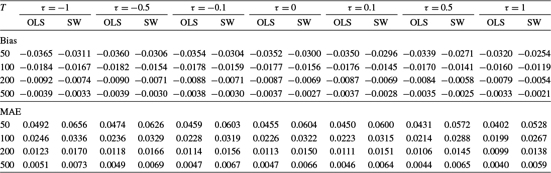


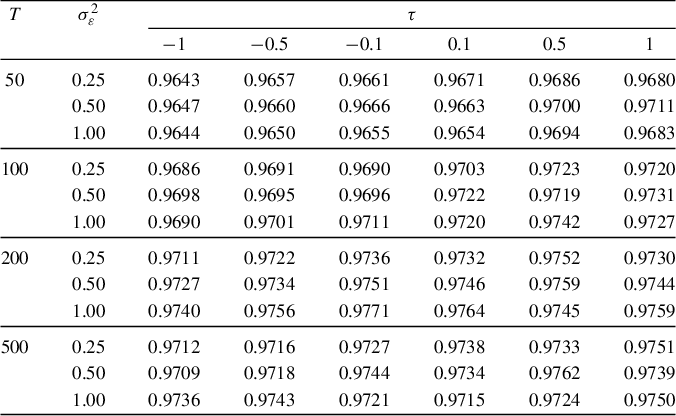

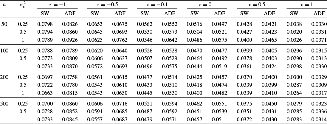


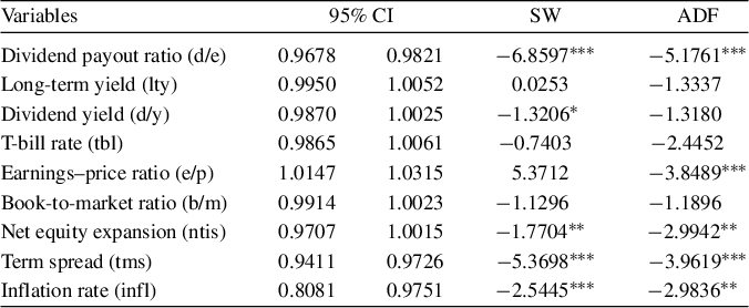
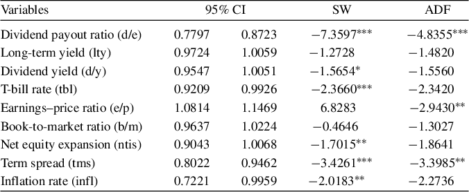


 Open access

