Noisy Retrospection: The Effect of Party Control on Policy Outcomes

ADAM M. DYNES; JOHN B. HOLBEIN

doi:10.1017/S0003055419000649

Noisy Retrospection: The Effect of Party Control on Policy Outcomes

Published online by Cambridge University Press: 04 November 2019

ADAM M. DYNES

and

JOHN B. HOLBEIN

Show author details

ADAM M. DYNES*: Affiliation:
Brigham Young University
JOHN B. HOLBEIN*: Affiliation:
University of Virginia
*: *Adam M. Dynes, Assistant Professor, Brigham Young University, adamdynes@byu.edu.
†John B. Holbein, Assistant Professor, University of Virginia, jh5ak@virginia.edu.

Article contents

Abstract
IMPORTANCE OF STUDYING PARTY CONTROL’S EFFECTS ON OUTCOMES
DOES PARTY CONTROL AFFECT OUTCOMES?
DATA
METHODS
RESULTS
DISCUSSION
SUPPLEMENTARY MATERIAL
Footnotes
References

Rights & Permissions

Abstract

Retrospective voting is vital for democracy. But, are the objective performance metrics widely thought to be relevant for retrospection—such as the performance of the economy, criminal justice system, and schools, to name a few—valid criteria for evaluating government performance? That is, do political coalitions actually have the power to influence the performance metrics used for retrospection on the timeline introduced by elections? Using difference-in-difference and regression discontinuity techniques, we find that US states governed by Democrats and those by Republicans perform equally well on economic, education, crime, family, social, environmental, and health outcomes on the timeline introduced by elections (2–4 years downstream). Our results suggest that voters may struggle to truly hold government coalitions accountable, as objective performance metrics appear to be largely out of the immediate control of political coalitions.

Information

Type: Research Article
Information: American Political Science Review , Volume 114 , Issue 1 , February 2020, pp. 237 - 257
DOI: https://doi.org/10.1017/S0003055419000649 [Opens in a new window]
Copyright: Copyright © American Political Science Association 2019

“Proponents of retrospective voting have simply assumed that there are real, persistent differences in … competence between competing teams of political elites.”

–Achen and Bartels (Reference Achen and Bartels2016, 158)

Whether citizens are able to hold government officials accountable is a foundational question for democracy. Indeed, theories of political accountability argue that citizen retrospection—the capacity of citizens to electorally punish and reward policymakers based on performance metrics—is vital for democratic well-being and prosperity (Ferejohn Reference Ferejohn1986; Fearon Reference Fearon, Przeworski, Stokes and Manin1999; Grant and Keohane Reference Grant and Keohane2005).^{Footnote 1} As a result of the importance of retrospective behavior, an abundant and ever-growing literature explores whether citizens respond when performance deteriorates [for an overview, see Healy and Malhotra (Reference Healy and Malhotra2013)]. In recent years, scholars have been critical of citizens’ capacity to fulfill their retrospective duty given their biased evaluations of economic performance (e.g., Bartels Reference Bartels2009; Huber, Hill, and Lenz Reference Huber, Hill and Lenz2012; Healy, Persson, and Snowberg Reference Healy, Persson and Snowberg2017) and propensity to react to forces that may be orthogonal to the control of politicians—such as sporting events (Healy, Malhotra, and Mo Reference Healy, Malhotra and Mo2010; Busby, Druckman, and Fredendall Reference Busby, Druckman and Fredendall2017),^{Footnote 2} shark attacks (Achen and Bartels Reference Achen and Bartels2016),^{Footnote 3} natural disasters (e.g., Healy and Malhotra Reference Healy and Malhotra2009), and policy decisions made by other actors (Sances Reference Sances2017). According to some, these types of responses constitute failures of retrospective voting (Achen and Bartels Reference Achen and Bartels2016).^{Footnote 4}

Scholars often take hope (Achen and Bartels Reference Achen and Bartels2016), however, when voters appear to also respond to metrics (seemingly) more directly in the control of elected officials. For example, there is evidence that citizens respond to dips in economic performance (Fiorina Reference Fiorina1978; Lenz Reference Lenz2013; Healy and Lenz Reference Healy and Lenz2014, Reference Healy and Lenz2017),^{Footnote 5} spikes in crime (Arnold and Carnes Reference Arnold and Carnes2012; Bateson Reference Bateson2012), increases in military deaths (Grose and Oppenheimer Reference Grose and Oppenheimer2007), decreases in school performance (Berry and Howell Reference Berry and Howell2007; Holbein Reference Holbein2016; Kogan, Lavertu, and Peskowitz Reference Kogan, Lavertu and Peskowitz2016), and changes to distributive spending (Chen Reference Chen2013), to name a few. While the literature is somewhat mixed about the capacity of voters to evaluate politicians’ performance (Healy and Malhotra Reference Healy and Malhotra2013), an underlying normative assumption is that public welfare would increase if retrospective voting over the proper performance metrics occurred (Key Reference Key1966; Kramer Reference Kramer1971; Fiorina Reference Fiorina1981; Ferejohn Reference Ferejohn1986; Fox and Shotts Reference Fox and Shotts2009, 1234; Arnold and Carnes Reference Arnold and Carnes2012, 962; Woon Reference Woon2012, 914). Simply put, retrospective voting in response to the ebbs and flows of policy outcomes (i.e., measures of societal well-being) is often seen as normatively desirable.

Underlying models of retrospective voting is the assumption that coalitions in power actually make a difference for the outcomes by which they are—or, according to some, should be—judged. Much of the literature takes as given that policy outcomes—like crime rates or the performance of the economy and schools—are appropriate measures of elected officials’ competence and performance. In this paper, we re-examine this assumption. Specifically, we present a reason for why the foundation of retrospective voting is tenuous: partisan coalitions don’t actually have clear and consistent effects on policy outcomes in the time between elections.

To demonstrate this, we estimate the effects of the party in power in US state governments on a number of policy outcomes (or proxies of societal well-being). Our objective is to explore the extent to which party control influences barometers of performance in the two to four years between elections in which voters must evaluate government performance. We choose to explore the role of party control, rather than the election of individual candidates, given that changes in party control are more likely to push a specific policy agenda—and hence move policy outcomes—in a different direction (Caughey, Warshaw, and Xu Reference Caughey, Warshaw and Xu2017). Our approach uses historical data from state legislatures and governors in the US matched to information on 47 policy outcomes^{Footnote 6} across six different sectors measuring economic, education, crime, social, environmental, and health/family outcomes. With these data, we show correlational evidence that Republican and Democratic states are descriptively different in the outcomes they realize in the short term. To rule out the possibility that these patterns are not a reflection of other factors, we use difference-in-difference and regression discontinuity models that leverage changes in party control and scenarios where one party holds marginal control. Our methodological approach, which is similar to other recent work on the effects of partisan control (Caughey, Warshaw, and Xu Reference Caughey, Warshaw and Xu2017; Hall, Feigenbaum, and Fouirnaies Reference Hall, Feigenbaum and Fouirnaies2017), shows that observational comparisons (and popular narratives) paint an oversimplified picture of the effects of party control.

Overall, we find that the party in power has almost no effects on economic, health/family, educational, crime, civic, and environmental outcomes within the timeline between elections. These null effects are precisely-estimated, systematic across many subgroups, and robust to a host of different checks. Moreover, they persist over multiple time periods and regardless of whether government is split or unified or whether the party has persistent power over time. Simply put, we fail to find evidence of causal differences in policy outcomes.

Our results make several important contributions. First, our empirical analysis directly addresses the important question of whether Democrats or Republicans lead to different levels of economic and social well-being, a question at the heart of most political contests in the US. Second, we expand the party effects literature (Erikson, Wright, and McIver Reference Erikson, Wright and McIver1989) to test whether party control’s impact on the ideological content of legislation (Caughey, Warshaw, and Xu Reference Caughey, Warshaw and Xu2017) extends downstream to metrics of economic performance and social well-being. In so doing, we also expand on past work on this specific question (e.g., Leigh Reference Leigh2008; Potrafke Reference Potrafke2018) by examining the effects of both gubernatorial and legislative control on a broader range of outcomes and with a research design that can identify more precise effects. Third, we test a fundamental assumption behind the normative arguments for retrospective voting—that the party in power affects the performance metrics that retrospective voters should use to hold public officials accountable.

Given these precisely estimated null effects, we conclude that voters who retrospectively vote political parties out of office based on the economy, or other performance metrics, may actually be responding to noise—i.e., factors that are largely out of the short-term control of politicians. This presents an important new wrinkle for understanding democratic accountability and calls into question the quality of retrospective voting. In order for citizens to truly hold elected officials accountable, more time may need to be allocated between when one party is in power and when accountability decisions are made. Alternatively, our findings suggest that elected state officials may be best judged by prospective judgments and evaluations of their actual legislative choices, an approach that requires higher levels of political knowledge and is currently underutilized by state voters (Rogers Reference Rogers2017) especially given deteriorating local media coverage (Shaker Reference Shaker2009). Overall, our results make an important contribution to the discussion of what voter retrospection can and should accomplish.

IMPORTANCE OF STUDYING PARTY CONTROL’S EFFECTS ON OUTCOMES

The empirical question of whether Democratic and Republican majorities in US state governments lead to different results in terms of economic and social well-being is key for understanding electoral politics and accountability, especially at the state level, for at least three reasons. First, it speaks directly to the central debate in most elections in the US’s two-party system: does one party systematically govern better than the other? Citizens, the media, and interest groups make key decisions based on which party they believe promotes better economic and social outcomes. Parties and candidates debate the merits of their platforms on this basis while political observers regularly claim that changes in party control will have major impacts on a state’s well-being (e.g., Berman Reference Berman2017; Nirappil Reference Nirappil2017). Not only do the parties propose different platforms, there is strong evidence that they also implement ideologically divergent legislation (Caughey, Warshaw, and Xu Reference Caughey, Warshaw and Xu2017). At the same time, state officials, like their national counterparts, claim credit for their state’s positive performance on economic and social measures (Turner Reference Turner2003; Volden Reference Volden2005) without necessarily strong evidence that their actions led to those desirable outcomes. In this way, our research question speaks to research on credit-claiming (Grimmer, Messing, and Westwood Reference Grimmer, Messing and Westwood2012) and whether state officials should claim credit for strong economic performance in the short window between elections.

Second, social scientists have long argued that political parties influence the overall health of the economy and other policy outcomes relevant to societal well-being [e.g., in American politics: Bartels (Reference Bartels2009), Hacker and Pierson (Reference Hacker and Pierson2010), and Faricy (Reference Faricy2011); in comparative politics: Alvarez, Garrett, and Lange (Reference Alvarez, Garrett and Lange1991) and Alesina and Roubini (Reference Alesina and Roubini1992); and in political economy more generally: Hibbs (Reference Hibbs1977), Chappell and Keech (Reference Chappell and Keech1986), and Alesina and Rosenthal (Reference Alesina and Rosenthal1995)]. Though most of this work focuses on national policy, a recent survey of political scientists studying American politics finds that they believe, on average, that state and local governments have at least some influence on economic outcomes in a two-year window and even greater influence on educational outcomes and crime rates (Caplan et al. Reference Caplan, Crampton, Grove and Somin2013). This belief, combined with the different platforms proposed by Democrats and Republicans at the state level, leads some scholars, such as Hacker and Pierson (Reference Hacker and Pierson2016), to claim that the reason Democratic states perform better than Republican ones is because “leading conservatives [at the state level] promote an economic model so disconnected from the true sources of prosperity.” Our article directly tests this important claim about partisan politics.

Third, identifying the impact of party control on measures of economic and social well-being has important implications for retrospective voting and electoral accountability. If party control has little to no effect on economic and social well-being in the short-term, then retrospective voting based on those metrics results in elected officials being rewarded and punished for outcomes outside of their control.^{Footnote 7} Thus, the results of this analysis test a key assumption favoring retrospective voting over policy outcomes.

As Achen and Bartels (Reference Achen and Bartels2016) explain, retrospective voting is “an attempt by voters to select the best available team of political leaders…through the auxiliary assumption that parties’ past performance in office can generate rational expectations about future performance” (98).^{Footnote 8} A central motivation for work on retrospective voting (e.g., Achen and Bartels Reference Achen and Bartels2016; Ashworth Reference Ashworth2012; Fearon Reference Fearon, Przeworski, Stokes and Manin1999; Ferejohn Reference Ferejohn1986; Healy and Malhotra Reference Healy and Malhotra2013; Healy, Persson, and Snowberg Reference Healy, Persson and Snowberg2017; Key Reference Key1966) and more generally on vote choice, including among state voters (Rogers Reference Rogers2016, Reference Rogers2017), is a normative concern about which factors should influence how people cast their votes. Often, the criteria for judging whether voters should use a metric for retrospective evaluations has tended to revolve around whether or not it is “clearly beyond the leaders’ control” (Achen and Bartels Reference Achen and Bartels2016, 142). Hence, scholars are concerned when voters punish elected officials for undesirable sporting outcomes (Busby, Druckman, and Fredendall Reference Busby, Druckman and Fredendall2017; Healy, Malhotra, and Mo Reference Healy, Malhotra and Mo2010) or other events (including those listed in the Introduction). In contrast, scholars often conclude that it is normatively desirable when they find evidence that policy outcomes plausibly linked to officials’ decision-making and efforts in office affect voters’ evaluations of policymakers and parties—e.g., on crime and economic performance see Arnold and Carnes (Reference Arnold and Carnes2012), on education see Berry and Howell (Reference Berry and Howell2007), and on disaster response see Gasper and Reeves (Reference Gasper and Reeves2011).

Retrospective Voting on Policy Outcomes in State Politics

Given the broad role that state governments can play in policymaking decisions in the US, it is plausible (for reasons we explain in the next section) that the performance of states’ economy, criminal justice system, schools, public health, and environment are affected by state policies. As such, these metrics of economic and social well-being may be good candidates for use in retrospective evaluations of state government’s performance. In addition, there is a body of work that suggests that voters do use economic metrics to evaluate governors.^{Footnote 9} In this literature, most find evidence of retrospective voting and evaluations even using statewide measures (e.g., Hansen Reference Hansen1999a, Reference Hansen1999b; Orth Reference Orth2001). However, there are gaps in this literature. For instance, only two publications also focus on economic retrospective voting in state legislative elections (Chubb Reference Chubb1988; Lowry, Alt, and Ferree Reference Lowry, Alt and Ferree1998). Though they fail to find a direct effect, Chubb (Reference Chubb1988) and others (Folke and Snyder Reference Folke and Snyder2012; Hogan Reference Hogan2005; King Reference King2001) find that governors’ popularity, which is affected by state economic performance (e.g., Cohen and King Reference Cohen and King2004), also affects the electoral success of same party state legislators to some degree. Further, though there is less work on whether non-economic outcomes have electoral effects in state politics, state politics scholars regularly expect state government policy to influence many of these outcomes (Grumbach Reference Grumbach2018; Hertel-Fernandez Reference Hertel-Fernandez2019; Moncrief and Squire Reference Moncrief and Squire2017; Potrafke Reference Potrafke2018; Rogers Reference Rogers2017), and as cited before, there is evidence that some of these non-economic metrics, like crime and educational performance, are used by voters to evaluate local governments. Given that local governments are creatures of the state and operate under the regulations and funding structure determined by state government, it would not be unexpected or wholly irrational for voters to also hold state officials accountable for criminal-justice and education policy since the proverbial buck (mostly) stops at the state government on these issues. In addition, survey work finds that Americans believe (on average) that state and local government are more than “somewhat influential” when it comes to crime rates and economic and educational performance (Caplan et al. Reference Caplan, Crampton, Grove and Somin2013), which suggests that such outcomes could be part of their voting calculations.

The question this article addresses with respect to retrospective voting is whether the party in power has the ability to affect the outcomes that voters might plausibly use—or that some scholars believe they should use—in evaluating party performance. If we find evidence that parties are able to affect economic and social well-being, then this would suggest that if citizens voted based on these metrics, they would be rewarding and punishing the party in power for outcomes within their control (at least to some degree). This result would clearly satisfy the normative arguments for retrospective voting as a tool for electoral accountability in state politics. On the other hand, if we fail to find evidence that party control has significant effects on economic and social well-being, it becomes less clear if retrospective voting is normatively desirable. If we struggle to find effects, voters probably will as well. Moreover, those who punish and reward the party in power for changes in economic, health, social, and criminal justice outcomes may be responding to noise—to factors outside of politicians’ control, like sporting events.

To be clear, even if party control has no detectable effect on societal well-being, it does not necessarily mean that retrospective voting is never welfare-enhancing. However, it changes the question on this topic to the following: is retrospective voting over short-term changes to economic and social outcomes still desirable even if the party in power had little impact on those outcomes? Perhaps, retrospective voting is still desirable at least as a form of “rough justice” (Fiorina Reference Fiorina1981, 4) in case officials were ever tempted to pursue extreme, risky, or imprudent policies (Somin Reference Somin2016, 103) that could wreck their state’s economy or decimate their public school or criminal justice systems.^{Footnote 10} But this view of retrospective voting as a means to prevent obviously disastrous policy decisions differs significantly from one in which it enables the electorate to behave as if it were a rational “god of [electoral] vengeance and reward” (Key Reference Key1955, 568). Moreover, as Achen and Bartels (Reference Achen and Bartels2016) argue, “the rougher [the justice] is, the less incentive reelection-minded incumbents will have to exert themselves on the voters’ behalf” (144). In sum, the results from this analysis help place bounds on the extent to which retrospective voting on policy outcomes leads to electoral accountability.

DOES PARTY CONTROL AFFECT OUTCOMES?

Overall, existing arguments and evidence do not leave clear expectations for whether we should expect changes in Republican and Democratic majorities in state government to lead to systematic differences in economic and social performance. Furthermore, there is a lack of systematic analysis of this question using methods that are better suited to identifying causal effects. As Achen and Bartels (Reference Achen and Bartels2016, 158) explain in their influential book on democratic accountability,

“[Retrospective voting] requires us to assume that there are real differences in economic competence between competing political teams. However, in light of the crucial importance of this assumption for the whole notion of retrospective selection, it is striking that it has never, as far as we know, been subjected to any systematic empirical examination. Proponents of retrospective voting have simply assumed that there are real, persistent differences in economic competence between competing teams of political elites.”

As Achen and Bartels suggest, the literature has for too long ignored whether policy coalitions can provide separation sufficient for voters to make substantive decisions at the ballot box.^{Footnote 11} Thus, it remains unclear whether this oft-assumed prerequisite for a functioning democracy is met. Theory and previous empirical work leave us with conflicting expectations, providing us with reasons to both suspect and be skeptical that parties affect social and economic well-being.

Reasons Why Party Control May Affect Outcomes

We begin with arguments for why Democratic and Republican control of US state government could lead to different policy outcomes. These arguments rest on two requirements: first, states must have sufficient power over relevant policies that could impact society, and second, political parties must implement different types of policies. There is justification to believe that both requirements are met.

Though the US federal government is often seen as much more influential over many policy domains than states (Kemp Reference Kemp1978; Rose Reference Rose1973; Winters Reference Winters1976), states still have significant autonomy in the types of relevant policies they can implement [for a review on this topic, see Moncrief and Squire (Reference Moncrief and Squire2017); also see Grumbach (Reference Grumbach2018)]. This is especially true in recent years, as the Federal government has experienced polarization and high degrees of gridlock and, as a result, much of the policy-making responsibility has shifted to the state level (Grumbach Reference Grumbach2018). In fact, in many policy areas and especially those in education, criminal justice, and social issues, states are the first or primary instigator of policy change (Moncrief and Squire Reference Moncrief and Squire2017, 101). For example, states (1) set tax rates for both individuals and businesses; (2) create regulations and incentive programs for particular industries; (3) control large portions of education funding and other education policies; (4) determine the criminal code and regulate local policing policies; (5) decide eligibility thresholds and benefit levels (within some guidelines) for several federal welfare programs, including Medicaid, the Children’s Health Insurance Program, and the Supplemental Nutrition Assistance Program; and (6) set minimum wage laws, among other potentially impactful policy decisions. Echoing many scholars of state politics, Rogers (Reference Rogers2017, 570) concludes that “state legislators have considerable authority over American lives. They determine who has the opportunity to vote, go to college, and even get married.”

The argument that states have significant policy scope is further shown in Caughey and Warshaw (Reference Caughey and Warshaw2015), who create a measure of policy ideology using data on 148 distinct policies across every state from 1936 through 2014. One clear finding from these data is that policies on a wide range of both social and economic issues vary significantly across states and time. This shows that states have the ability to pursue a wide range of policies that many argue (especially, advocates for and against these policies) should impact society and economic performance. Indeed, there are massive literatures in the social sciences that attempt to identify the effects of all of these state-controlled or influenced policy changes on society, suggesting that many scholars (or at least practitioners and policymakers) anticipate that these policy changes have effects.

A recent survey of political scientists who study American politics also supports the stance that states have significant influence on policy outcomes (Caplan et al. Reference Caplan, Crampton, Grove and Somin2013). When asked to indicate how much influence state and local governments “have over whether the economy gets stronger or weaker during the next two years,” the average response was halfway between “somewhat influential” and “not very influential” (761). Notice that this was asking specifically about influence in just a two-year time period. Scholars may have rated state and local government even more influential if asked about longer time periods. Political scientists credited state and local governments with even greater influence when asked “how much influence [they] have over crime rates” and “how well the public schools educate their students” (761). For both questions, the average response was halfway between “very influential” and “somewhat influential.” In sum, there are both scholars and scholarship that anticipate state governments to influence economic and social outcomes even in the short-term.

In addition to states controlling important policy levers, the two major parties competing for state offices propose and implement ideologically divergent policies (Coffey Reference Coffey2011), with Democrats favoring more redistribution, spending, and progressive taxation since the New Deal era (Dye Reference Dye1966; Erikson, Wright, and McIver Reference Erikson, Wright and McIver1989; Jennings Reference Jennings1979). Republican and Democratic state legislators also vote quite differently from one another, even when representing ideologically similar districts (Shor and McCarty Reference Shor and McCarty2011). More importantly, there is compelling empirical evidence using difference-in-difference and regression discontinuity designs that a marginal shift to Democratic control of a legislative chamber or governor’s office leads to an immediate ideological shift to the left in the type of legislation that passes (Caughey, Warshaw, and Xu Reference Caughey, Warshaw and Xu2017). This approach accounts for other factors that could outweigh the effects of partisan majority control such as public opinion, economic conditions, and federal policies. As mentioned above, countless policy advocates and candidates anticipate and claim that these ideological shifts in legislation will impact economic and social outcomes.

Finally, there is a scattered empirical literature that suggests that party control affects policy outcomes in some instances. In a review of the literature at the national, state, and local levels, Potrafke (Reference Potrafke2018) finds evidence for a partisan effect on some policies and policy outcomes but not others.^{Footnote 12} However, this literature faces three major limitations. First, the vast majority of studies in this literature simply relates party control with policy outcomes, conditioning on a few observable characteristics.^{Footnote 13} Second, studies in this literature, including those that implement more rigorous research designs, only focus on control of the executive branch. This may give us an incomplete view of the effect of partisan control given the important role that state legislatures play in the policymaking process vis-à-vis governors (Kousser and Phillips Reference Kousser and Phillips2012). Third, these studies only focus on a small set of metrics at a time; indeed, studies in this domain frequently only focus on a single policy outcome at a time.^{Footnote 14} This may result in a “file-drawer” problem—a potential bias in a literature due to researchers’ and journals’ tendency to publish statistically significant findings but not null findings (Franco, Malhotra, and Simonovits Reference Franco, Malhotra and Simonovits2014). If research on the effects of party control only ever focuses on a single policy outcome, it could be possible that the literature includes many spurious findings, overstating the effects of party control.

The one exception to this last trend is Leigh (Reference Leigh2008). This study provides the most extensive analysis of the effects of party control on legislative outputs and outcomes, focusing on gubernatorial partisanship. Using a regression discontinuity design, Leigh (Reference Leigh2008) fails to find evidence that the partisanship of the governor matters on 16 outcomes, including measures of crime, income, and employment. Overall, Leigh concludes that governors’ partisanship has little effect on metrics of social well-being. Missing from this analysis, however, is whether party control of state legislatures matters. Indeed, Leigh (Reference Leigh2008) conjectures that party control of state legislatures may matter more for policy outcomes given the electoral incentive for governors to be more centrist (Reed Reference Reed2006). In this article, we address these issues by using two compelling causal identification strategies that provide us with very precise estimates, exploring executive and legislative control, looking at a longer list of policy outcomes together, expanding the time series, and applying the results to broader concerns in the political science literature about party control and electoral accountability.

Though there are reasons to expect that party control affects economic and social outcomes, important gaps in the literature remain (which we help fill). In addition, and as discussed below, there are reasons to be skeptical of an effect.

Reasons Why Party Control May Not Affect Outcomes

A first reason why party control may not affect outcomes is that the two to four-year timeline after a change in party control may be too short for the full effects of policy changes to take place. It is possible that the parties’ competing legislative agendas do have different effects but take time to develop. On the other hand, Caughey, Warshaw, and Xu (Reference Caughey, Warshaw and Xu2017) find that changes in party control lead to immediate changes in the ideological composition of the policies that are passed at the state level. Moreover, examining effects one year downstream is the norm in education (e.g., Angrist, Pathak, and Walters Reference Angrist, Pathak and Walters2013; Chiang Reference Chiang2009), health (e.g., Finkelstein et al. Reference Finkelstein, Taubman, Wright, Bernstein, Gruber, Newhouse, Allen and Baicker2012; Newhouse and Group Reference Newhouse1993), social welfare (e.g., Jardim et al. Reference Jardim, Long, Plotnick, Van Inwegen, Vigdor and Wething2017), and criminal justice (e.g., Ludwig and Cook Reference Ludwig and Cook2000; Yokum, Ravishankar, and Coppock Reference Yokum, Ravishankar and Coppock2017) research. Similarly, state-level agencies and legislative analysts regularly predict that changes in fiscal and other policies will have short-term effects, which our research design should pick up.

Second, though Caughey, Warshaw, and Xu (Reference Caughey, Warshaw and Xu2017) find that changes in party control lead to immediate changes in the ideological composition of the policies that are passed at the state level, these effects were modest in size. Marginal changes in party control did not lead to extreme changes in legislation overall, which may mean that party control will have small effects on the economy and social well-being. Grossman (Reference GrossmanForthcoming) makes a similar argument specifically about Republicans’ dominance in state government in recent decades. On the other hand, Caughey’s use of an aggregate measure of legislation’s liberalism could hide a partisan effect that is pronounced on a few key issues that potentially have large effects.

Third, the most comprehensive study to date using methods that can isolate a causal effect fails to find much evidence that party control of the governor’s office affects economic outcomes, at least in a systematic way (Leigh Reference Leigh2008). If governors have little to no effect, then perhaps state legislatures do, too. At the same time, our analysis has additional power to identify effects.

Fourth, though Republicans and Democrats propose and implement different policies, perhaps the bundle of policies they implement have similar effects on some outcomes either because there are multiple ways to achieve such effects (e.g., Republicans’ limiting access to abortion clinics and Democrats’ increasing access to birth control may both lower abortion rates) or because individual policies within each party’s bundle counteract one another.

A final reason why we may fail to find an effect is if retrospective voting constrains the set of policies that politicians from either party are willing to pursue. If politicians believe that citizens will punish and reward them for economic and social performance, it may cause them to put forward similar efforts and policies to effect popular outcomes, leading to no differences in economic performance between Democrats and Republicans, ceteris paribus. Though it is likely that both Republican and Democratic politicians fear the “rough justice” (Fiorina Reference Fiorina1981, 4) that would follow any policy disasters, we do not believe this reason would be a sufficient explanation for a lack of difference in social performance across the two parties since the parties consistently pursue and implement ideologically different policy agendas (Caughey, Warshaw, and Xu Reference Caughey, Warshaw and Xu2017). While there are forces that push the two parties toward the middle in terms of the policies they propose (Downs Reference Downs1957), there are also forces that drive them apart (Grofman Reference Grofman2004), which results in different policies passed in practice (Caughey, Warshaw, and Xu Reference Caughey, Warshaw and Xu2017). In other words, if the threat of retrospective voting leads both parties to put forward similar effort to improve economic and social well-being, that effort looks systematically different between Republicans and Democrats even in the most moderate states where party control is marginal. As such, we do not believe that politicians’ fear of retrospective voters would explain a null result in our analysis. (At most, this fear limits politicians from pursuing their riskiest proposals.)

DATA

To examine whether Democratic or Republican control leads to different outcomes in terms of social and economic well-being, we use data from the Correlates of State Policy Project Database (CSPPD), which is housed at the Institute for Public Policy and Social Research at Michigan State University (Jordan and Grossmann Reference Jordan and Grossmann2019). These data provide the party in power for both chambers and Governorships in all states (our independent variables) as well as data on policy outcomes (our dependent variables) from 1960 to 2016.

In this article, we examine primarily 28 outcomes that capture states’ economic, health/family, civic, criminal, educational, and environmental well-being.^{Footnote 15} Though the variables that we use vary in terms of their availability over time (with the largest window being from 1962 through 2019 and the shortest from 1991 through 2008), all of the variables primarily overlap the time period when Caughey, Warshaw, and Xu (Reference Caughey, Warshaw and Xu2017) find that partisan control had the largest effect on the policies that are passed. The economic outcomes available in the CSPPD include standard measures of average income (real, per-capita), inflation (CPI),^{Footnote 16} unemployment, growth (GSP), quarterly housing prices, population growth, the number of businesses, the performance of the agriculture sector, and (as measures of economic inequality) the fraction of income held by the top 1 and 0.1%. The available health/family outcomes include measures of health spending (per capita), the number of new immigrants, the abortion rate, divorce rate, and the birth rate. The civic outcomes include voter turnout and the number of felons ineligible to vote. Crime-related outcomes include measures of the auto theft, murder, property crime, rape, robbery, and violent crime rates. Education outcomes include school attendance and the percent of the population with a high school diploma. Finally, our environmental outcomes capture the amount of CO₂ emissions, energy usage by the business sector, and the price of residential energy. These outcomes provide a thorough picture of the potential effect of party control on multiple dimensions of societal well-being.

In examining the effect of party control on policy outcomes, we are trying to strike a delicate balance in which outcomes to include. On the one hand, our objective is to be as thorough as possible to avoid any potential “file-drawer” problems that could result by examining only a few policy outcomes (Franco, Malhotra, and Simonovits Reference Franco, Malhotra and Simonovits2014). At the same time, however, we do not wish to introduce outcomes that are irrelevant to party control of state government or for retrospective voting. This might skew our conclusions in the opposite direction and mute party control’s effects.

As such, we have sought to focus on outcomes that could plausibly be linked to changes made by party coalitions or that voters can/do/should use to evaluate policymakers in elections. Concerning the former, the outcomes examined here and in the Online Appendix all relate (at least to some degree) to the broad scope of policies that state governments have influence over, as described above in the section “Reasons Why Parties May Affect Outcomes.” This is particularly the case with the economic measures such as per capita income, unemployment, gross state product, number of businesses, and income inequality (in addition to gender income gap, business climate, state credit ratings, and poverty rates, which we examine in the Online Appendix). All of these are linked to states’ ability to determine redistributive policies, taxation, and business incentives and regulations, policies over which the parties disagree and that vary significantly across states. Likewise, the crime-related outcomes relate to states’ vast powers over the criminal code and law enforcement while education outcomes relate to states’ control of statewide K-12 policies and large portions of K-12 funding.^{Footnote 17} With the health and family outcomes, such as abortion and divorce rates, states are the primary source of variance in abortion and divorce laws in the US. Finally, the outcome measures dealing with the economy, crime, education, and immigration have also been the focus of past work on the effects of party control at the state level (Leigh Reference Leigh2008; Potrafke Reference Potrafke2018).

Concerning how these outcomes relate to retrospective voting, it is important to note that many of the outcomes we explore—such as individual income, school performance, educational attainment, health, crime, productivity, and unemployment—are valence issues with clearly desirable directional changes, be it for higher (e.g., income) or lower (e.g., crime) levels.^{Footnote 18} As such, these issues are candidates for use in retrospective evaluations, especially since there is a plausible link between these outcomes and state policy. Moreover, past work finds that many of these outcomes are already used by voters in different settings (Arnold and Carnes Reference Arnold and Carnes2012; Healy and Malhotra Reference Healy and Malhotra2013; Achen and Bartels Reference Achen and Bartels2016; Holbein Reference Holbein2016), especially several of the economic outcomes in gubernatorial elections—e.g., per capita income (Lowry, Alt, and Ferree Reference Lowry, Alt and Ferree1998),^{Footnote 19} unemployment (Ebeid and Rodden Reference Ebeid and Rodden2006), and inflation (Cohen and King Reference Cohen and King2004). Finally, analyzing the effects of party control on a broad range of outcomes addresses the important, normative question of which outcomes, if any, should voters use to evaluate policymakers and the party in power.

We realize some readers may still have concerns with which outcomes are or are not included in our analysis. However, the story we would tell would likely remain the same whether we removed some outcomes from the analysis or added others. As we show below and in the extensive Online Appendix, the null results are remarkably consistent across outcome types including composite scores of outcomes in similar policy domains.

In our analyses, we focus on the effect of party control on outcomes up to four years after party control changes.^{Footnote 20} As we mention above, our primary interest is in examining the effects of party control on the time line introduced by elections. Though it is feasible that party effects need time to manifest themselves, electoral decisions based on these possible effects have to be made by voters in the window between elections, which is generally two years for legislative elections and four years for gubernatorial ones. That said, in the Online Appendix we set aside our election time line and also examine outcomes up to eight years downstream.^{Footnote 21} The results do not change with additional time. Also, as discussed earlier, previous work has found evidence of short term effects (Potrafke Reference Potrafke2018) and examining effects one year after a policy change is the norm in many public policy literatures on outcomes similar to the ones we examine here. Based on all of this, it is plausible that we might observe party effects within the timeline we use.

Bivariate Comparisons

Before outlining our identification strategy, it is useful to examine what the simple raw comparisons show. While not causal, this exercise gives us a way to benchmark to the comparisons made in previous research at the federal and state levels and to public discussion about the performance of the two political parties. At first blush, the empirics tend to support the idea that the party in power affects short-term societal well–being.

Figure 1 displays the observational relationship between party control of different branches of state government (independent variable) and the levels of several outcome measures (dependent variable), controlling only for the party in control in the other respective branches of government. As can be seen, 69 (61.6%) out of the 112 tests (4 treatments by 28 outcomes) show a statistically significant party difference. This holds true even if we adjust for multiple comparisons (48.2% significant). Turning to the bottom right panel, we can see that states with unified Democratic governments have lower income, higher unemployment, lower voter turnout, higher murder rates, and lower diploma rates (to name a few). The observational patterns here suggest that there may be something important about the political party in power in determining policy outcomes—and these patterns look unfavorable for states controlled by Democrats.

FIGURE 1.

Simple Relationship Between Democratic Control & Policy Outcomes

Figure displays coefficient plots of the simple estimates between party control in the three bodies (upper, lower, governor) and outcome measure levels in the second year. Point estimates are shown with dots and 90% (95%) confidence intervals with thick (thin) bars. The outcomes are standardized simply to allow for a similar scale in the figure.

Observational patterns do not mean that the party in control caused these outcomes. States are potentially different for a host of reasons unrelated to the party in control of state government. However, if these outcomes are used in voters’ electoral decisions, different patterns in the performance of policy outcomes may feed into future electoral results. For example, a large body of work finds that per capita income is a factor in gubernatorial elections and evaluations (e.g., Ebeid and Rodden Reference Ebeid and Rodden2006; Niemi, Stanley, and Vogel Reference Niemi, Stanley and Vogel1995), and in Figure 1, Democratic control is associated with lower income in three of the four panels. But therein lies one of the fundamental problems with observational studies on party control and policy outcomes that have dominated previous research: the presence of retrospective voting implies endogeneity, muddying the ability to draw a clear causal conclusion over which party is producing better policy outcomes.

METHODS

To estimate the causal effect of partisan control on metrics of economic and societal well-being, we use two complementary comparisons. The first uses the panel nature of our data to estimate difference-in-difference models. The second uses naturally–occurring, as-if random assignment of party control to estimate regression discontinuity models. Our approach follows recent work that also examines the effect of partisan control at the state level on politically relevant outcomes (Caughey, Warshaw, and Xu Reference Caughey, Warshaw and Xu2017; Hall, Feigenbaum, and Fouirnaies Reference Hall, Feigenbaum and Fouirnaies2017).

Typically, a difference-in-difference that leverages state-level changes includes two-way fixed effects as outlined in equation (1), where D _st represents the treatment of interest [whether a state (s) is governed by democrats in a given year (t)], O _st represents the outcome levels we explore, and α _t and γ _s represent year and state fixed effects (respectively). However, in our application there are reasons to move beyond this specification. A standard check in the difference-in-difference literature involves looking for treatment effects on outcomes before treatment has occurred (e.g., Wing, Simon, and Bello-Gomez Reference Wing, Simon and Bello-Gomez2018). When we run this specification in the Online Appendix, we find some signs of imbalance across the treated and the untreated units. Examining our 28 lagged outcomes across our three treatments (Democratic House, Senate, and Governor) reveals that 12% of our tests show signs of statistically significant effects in the year before treatment is observed. While these effects are small [median effect = 2% of standard deviation (σ)] and many do not clear multiple comparison thresholds (only 4.8% of our tests do), there are still reasons to want to move to a more sophisticated specification to purge out potential sources of bias.^{Footnote 22}

(1)

$${O_{st}} = {\beta _0} + {\beta _1}{D_{st}} + {\alpha _t} + {\gamma _s} + {\varepsilon _{st}}.$$

Hence, our preferred difference-in-differences models consist of a relatively straightforward extension of equation (1) that includes state and year fixed effects and flexible linear time trends for each state. This is a standard recommendation in the difference-in-difference literature, especially when the two-way fixed effects models fail to produce desired levels of balance (e.g., Wing, Simon, and Bello-Gomez Reference Wing, Simon and Bello-Gomez2018). This approach absorbs all observed and unobserved factors that remain constant within states (e.g., political culture, social capital, rigid political institutions, etc.) and are shared within certain years (e.g., recessions, campaigns, etc.), and trends that vary across states (e.g., the natural trajectory on our outcomes). When we include the (linear) state-specific time trends, we are running the specification listed in equation (2).^{Footnote 23}

(2)

$${O_{st}} = {\beta _0} + {\beta _1}{D_{st}} + {\alpha _t} + {\gamma _s} + {\gamma _s} \times t + {\varepsilon _{st}}.$$

The virtue of this approach is that allows for even better causal identification and more precise estimates. The inclusion of state-specific time trends allows us to relax the (sometimes tenuous) parallel trends assumption key to difference-in-difference specifications. Here our identifying assumption is that our outcomes deviate from common year effects by following the linear trend captured by the interaction term. Under this assumption, identification comes from sharp deviations from otherwise smooth state-specific trends. This is a weaker assumption than what is required in a model with just state and year fixed effects (Angrist and Pischke Reference Angrist and Pischke2008, Reference Angrist and Pischke2014). This bears itself out in the data. When we go through the same specification tests that we did with the two-way fixed effects model, we see even better balance. Under this specification, only 4.8% of our tests show signs of statistically significant effects in the year before treatment. Further, these imbalances are even smaller than those in the two-way fixed effects specification (median effect = 0.0007σ) and none of these imbalances clear multiple comparison thresholds. Given these desirable properties, our main difference-in-difference specification is the one with linear time trends. We do, however, run many robustness tests to this preferred specification below and in the Online Appendix.^{Footnote 24}

Supplemental Method: Regression Discontinuity Design

To complement our difference-in-difference design, we use a second identification strategy. This approach leverages exogenous variation around the cutoffs determining which party is in power of the two legislative chambers and the governorship to estimate regression discontinuity design (RDD) models. Under a regression discontinuity framework, observations that are sufficiently close to an arbitrary discontinuity are separated primarily by exogenous shocks (Butler and Butler Reference Butler and Butler2006; Imbens and Lemieux Reference Imbens and Lemieux2008; Lee Reference Lee2008; Lee and Lemieux Reference Lee and Lemieux2010; Lemieux and Milligan Reference Lemieux and Milligan2008). Regression discontinuity models benefit from continuity in potential outcomes around the cutoff. Given modest assumptions, RDD models produce unbiased local average treatment effects that benchmark well with causal estimates from randomized–control trials (Buddelmeyer and Skoufias Reference Buddelmeyer and Skoufias2004; Green et al. Reference Green, Leong, Kern, Gerber and Larimer2009; Lee and Lemieux Reference Lee and Lemieux2010).

The party control cutoffs allow us to estimate the effect of legislatures and governorships being marginally controlled by Democrats by comparing those to bodies marginally controlled by Republicans. Following previous work estimating the effects of party control on policies passed (Caughey, Warshaw, and Xu Reference Caughey, Warshaw and Xu2017), our first RDD analyses estimate a standard RDD model for each of three cutoffs (upper chamber, lower chamber, and governorship) individually. The key input in these models is which party is in power in a given year for that respective body. This variable takes the value of one when a state legislative chamber or governorship was controlled by Democrats and zero otherwise. In our RDD models, we specify the running variable in two ways: first, as the proportion of seats above the party control threshold for Democrats and second, using the three alternate specifications of the running variable suggested by Hall, Feigenbaum, and Fouirnaies (Reference Hall, Feigenbaum and Fouirnaies2017).

Our base RDD model takes the specification in equation (3). In this specification, we are modeling our outcomes (O) in a given state (s) and year (t) as a function of party control (D) and proximity to party control (P). In our single-dimension RDD models, we specify the running variable with a local kernel-smoothed function g(•) and use the optimal bandwidth suggested by Calonico, Cattaneo, and Titiunik (Reference Calonico, Cattaneo and Titiunik2014). (We also check across different specifications of the running variables and a wide range of bandwidths.) Our preferred model specification also adds a state (γ) and year (α) fixed effect. These are identified based on states that switch party control at least once over the period studied. Hence, our model is analogous to an RDD combined with a difference-in-difference. This approach increases our level of statistical precision and allows us to absorb state- and time-constant observed and unobserved factors that may remain imbalanced around the cutoffs. (Again, our results are robust to omitting these fixed effects.)

(3)

$${O_{st}} = {\beta _0} + {\beta _1}{D_{st}} + g\left( {{P_{st}}} \right) + {\alpha _t} + {\gamma _s} + {\varepsilon _{st}}.$$

If the party power discontinuity sorts legislatures in an as-good-as random manner within states, the RDD specification will provide the causal effect of (marginal) political party power in state legislatures. This estimate will be unbiased by confounders or simultaneity because legislatures fall on either side of the party control cutoff as-good-as randomly within a narrow bandwidth. To examine whether our discontinuity satisfies the implications of local randomization, we conduct the standard RDD specification checks in the Online Appendix, finding little evidence of covariate imbalance or precise sorting around the cutoff. However, to be safe we also run donut regression discontinuity models that deal for any heaping-induced bias near the cutoff (Barreca et al. Reference Barreca, Guldi, Lindo and Waddell2011; Barreca, Lindo, and Waddell Reference Barreca, Lindo and Waddell2016).

The setup in equation (3) does not fully capture the potential effects of unified government, but specifying a regression discontinuity model for unified party control is challenging. It is not clear how to specify how close a government is to unified control since there are three running variables at play—one each for the house, senate, and governor. We take two complementary approaches to doing so. The first, which we focus on in the article text, specifies proximity to Democratic control with the minimum of the house, senate, or governor scores. This follows an approach in economics (Ahn and Vigdor Reference Ahn and Vigdor2014) and political science (Holbein Reference Holbein2016). The logic here is that in a situation where multiple running variables determine a single treatment, the minimum score shows how far the unit has to go to either be pulled over the threshold for treatment (if it is below the treatment cutoff) or how far it has to deteriorate to fall back into the control (if it is above the treatment cutoff). This approach assumes that the three running variables move in an order-preserving manner. Recognizing the limitations of this approach, we leverage a second technique that conceptualizes treatment as truly multi-dimensional. That is, it conceptualizes treatment as being comprised of the interaction of three treatment variables and three running variables. This approach includes all of these (and their interactions) into one multiple-regression discontinuity model. This follows the suggested approach of Papay, Willett, and Murnane (Reference Papay, Willett and Murnane2011). The one drawback of this approach is that it stretches the state-level panel to its limits in terms of common support. With a six-way interaction (and its various sub-components) the resulting MRDD models come with inflated standard errors. While neither of these approaches is perfect, together these allow us to wrap our arms around a regression discontinuity approach for looking at the effects of unified party control on policy outcomes.

While our regression discontinuity models come with (perhaps) better internal validity than our difference-in-difference specifications, they do come with the cost of reduced statistical power and, perhaps, generalizability. Given that neither of our approaches is perfect, we rely on both below. Ultimately, we are reassured that both give us a very similar answer.

Statistical Precision and Multiple Hypothesis Corrections

Before showing our results, we take a moment to discuss two issues that influence our ability to answer the question at hand: statistical power and multiple comparisons.

In addition to being concerned about identifying the causal effect of party control on policy outcomes (within the window surrounding elections), we also pay specific attention to the precision of our results. After all, imprecisely-estimated null effects may not teach us very much about the effect of interest and significant effects that come from underpowered designs may be plagued by Type S (significance) and Type M (magnitude) errors (Gelman and Carlin Reference Gelman and Carlin2014). To help allay these concerns, we do several things. First, we use difference-in-difference specifications that are better powered than our regression discontinuity models. Second, we reduce noise in our models by creating factor-weighted scales that capture how well a state is doing on our six policy dimensions. Doing so reduces measurement error and estimation error as a result (Anderson Reference Anderson2008; Ansolabehere, Rodden, and Snyder Reference Ansolabehere, Rodden and Snyder2008; Caughey, Warshaw, and Xu Reference Caughey, Warshaw and Xu2017). Third, in some of our models, we explicitly control for our outcomes in previous periods. We do this by either explicitly including lags in our models or, alternatively, by looking at changes in our outcomes, which is logically equivalent. As we show below, this improves our precision substantially. Fourth, in our results below, we discuss not only the statistical significance of our results, but also their substantive size. In so doing, we pay attention to our 95% confidence intervals. This allows us to discuss what effect sizes we are able to rule out; an approach intuitively similar to the equivalence testing approach suggested by Hartman and Hidalgo (Reference Hartman and Hidalgo2018) and others in the literature on null effects and statistical/substantive significance (Gross Reference Gross2015; McCaskey and Rainey Reference McCaskey and Rainey2015; Rainey Reference Rainey2014). In our models below, we use Hartman and Hidalgo’s default values for equivalence testing (36% of a standard deviation) and test whether our effects are distinct from that benchmark. We do this as what constitutes a meaningful effect is not well defined in our application. However, we also mention minimum detectable effects (MDEs)—an increasingly common standard approach in the literature (e.g., Haushofer and Shapiro Reference Haushofer and Shapiro2016). Ultimately, providing MDEs allows the reader to make conclusions about the types of effects that we can confidently rule out. Finally, in our robustness checks for our RDD models specifically, we vary the bandwidth around our cutoff—increasing our power by using more data around the cutoff (an approach recommended by Lee and Lemieux Reference Lee and Lemieux2010). Our substantive conclusions remain similar from very narrow to very wide bandwidths. However, we are substantially better-powered in wider bandwidths (while still preserving covariate balance, as we show in the Online Appendix).

The second issue, multiple comparisons, follows from our need to examine multiple outcomes, which is due, in part, to avoiding a file-drawer problem (Franco, Malhotra, and Simonovits Reference Franco, Malhotra and Simonovits2014). Scholars have long noted that when examining multiple outcomes, some estimates will be statistically significant simply by chance (e.g., Dudoit et al. Reference Dudoit, Shaffer and Boldrick2003; Shaffer Reference Shaffer1995). Given the results that we present below—overwhelmingly, coefficients not statistically different from zero—we want to be careful to not over-interpret the presence of some coefficients that are statistically significant by simple random chance. We make an effort to note when effects cross standard significance levels and whether this is robust to the standard multiple hypothesis testing adjustments [i.e., the Bonferroni, Sidak, and free step-down resampling corrections; See Westfall and Young (Reference Westfall and Young1993); Jones, Molitor, and Reif (Reference Jones, Molitor and Reif2018)].^{Footnote 25} Because we are making the case for the null, the conservative approach is actually to not make any adjustments to the p-values. Hence, this is why we draw such attention to the unadjusted p-values throughout the text.

RESULTS

To preview our results, we find evidence that the party in power has little to no immediate effect on outcomes in the economy, education, environment, health/family, crime, and civic sectors. These estimates are quite precise and allow us to rule out even very modest effects. Simply put, Democrats and Republicans appear to be equal in terms of their ability to produce a wide range of policy outcomes associated with overall well-being or social prosperity on the timeline introduced by elections. This holds across all of our difference-in-difference and RDD setups as well as across a multitude of robustness checks.

Difference-in-Difference Estimates

We start by exploring the effect of having a single chamber switching from Republican to Democratic party control. These estimates are shown in Figure 2, which focuses on the four year downstream estimates to allow for effects to materialize over a longer time within the window of elections.^{Footnote 26} As can be seen, for the most part, the effect estimates are not statistically significant at the unadjusted 5% significance level—82/84 (97.6%) of the coefficients (28 outcomes by three chambers) estimated have p-values greater than 0.05. This is slightly less than what we would expect by chance alone. The two exceptions are unemployment_House and population growth_Governor. However, neither of these two coefficients clear the Bonferoni, Sidak, or free step-down resampling multiple comparison levels. Further, the effects estimates are small; the average effect size is a paltry 0.8% of a standard deviation (σ) and the median effect size is only 0.6% σ. Moreover, most of these coefficients are quite precise. In all cases, our 95% confidence intervals allow us to rule out effects that are much smaller than Hartman and Hidalgo’s default values for equivalence testing (36% of a standard deviation).^{Footnote 27} Overall, the median upper bound for our MDEs is 6.7% of a standard deviation and the median lower bound for our MDEs is −5.5% of a standard deviation. This is impressive given that these effect sizes are traditionally considered to be quite small (Cohen Reference Cohen1992). The most precise null estimate is for CPI (with the CO₂ emissions estimate close behind); the least precise null estimate is school attendance (which makes sense given the shorter time series for this measure). The results, in most cases, are not close to being statistically significant at traditional levels, with the average p-value being 0.53 (median = 0.54). There appear to be no systematic effects by chamber, timing, issue domain, or individual outcomes themselves. Regardless of what set of outcomes you include in an overall evaluation of the effect of party control, the story is the same: switching from one political party in control (Democrats) to the other (Republicans) has surprisingly small to non-existent causal effects on policy outcomes between elections.^{Footnote 28}

FIGURE 2.

Difference-in-Difference Estimates of Single Chamber Changes to Democratic Control (Fourth Year)

Figure plots standardized coefficient estimates (points) and corresponding 90% (thick) and 95% (thin) confidence intervals for the difference-in-difference estimates for the effects of each individual chamber. Coefficients are faceted by policy area and broken by individual chamber within facets. Three reference lines are shown that allow for tests against a null hypothesis of a zero effect (center) and the default equivalence testing values suggested by Hartman and Hidalgo (Reference Hartman and Hidalgo2018) (right and left). Standard errors are clustered at the state level. The numbers used to make this plot—including the exact coefficients, standard errors, p-values, 95% confidence intervals, and sample sizes—are in the Online Appendix.

These precise null effects results are remarkably robust to—and even strengthened by—alternate specifications, which we show in the Online Appendix. For example, if we look at changes in our outcome variables, our already precise nulls become even more precise. Under this specification, again, our results show effects that are small (median β = 0.2% σ), not statistically significant (95.2% not significant at unadjusted levels; 98.8% not significant at multiple hypothesis testing levels), and that allow us to rule out substantively meaningful effects. All effects are statistically and substantively distinct from Hartman and Hidalgo’s default values for equivalence testing. However, under this specification we are able to be much more precise than in our previous model specifications. The median MDE is a paltry −1.9% of a standard deviation (on the low end) and 2.6% of a standard deviation (on the high end). In fact, in all of our models we can rule out effects of 20% of a standard deviation. In 85% of our models, we can confidently rule out effects as small as 10% of a standard deviation, and in a full two-thirds of our models, we can confidently rule out effects as small as 5% of a standard deviation. This conclusion of null effects also holds if we look at composite outcomes—that is, if we create scales of how well a state is doing in terms of its economy, schools, etc. in a given year.^{Footnote 29} Our results are also robust to iteratively holding out individual states—a common check to help rule out the possibility that individual outliers may be driving results.

Our results are also robust to changes in how we conceptualize the treatment. For example, instead of using an indicator variable to categorize whether Democrats are in control, we can include the continuous running variable measure to capture by how much they do (or do not) have control. This allows us to see whether having more dominant control in a chamber/governor’s office influences policy outcomes. When we run this check, the results remain the same. Out of the 336 coefficients estimated (28 outcomes × 3 chambers × 4 time periods) only 16 (4.8%) are statistically significant at the unadjusted 5% level, with none of these clearing multiple comparisons thresholds. Moreover, the coefficient estimates are small: being tightly centered around zero (mean = −0.4% σ; median = −0.11% σ).^{Footnote 30} Simply put, holding more of a chamber (or a stronger position in the governor’s chair) has no effect on policy outcomes in the window introduced by elections.

But, perhaps having unified party control across all three chambers is what provides parties with the ability to produce meaningful differences in policy outcomes. In practice, this is done by creating three indicators—one for whether state government is unified Democrat, the next for whether it is unified Republican, and the third for whether it is divided government. Given the substantive interest between unified Republican or Democratic control, in the figures below we present the results for a model with the unified Republican category as the left-out value.^{Footnote 31}

Figure 3 shows our difference-in-difference estimates for the effect of unified Democratic control compared to unified Republican control.^{Footnote 32} As can be seen, none of the effect estimates is statistically significant at the unadjusted 5% significance level, much less at the Bonferoni, Sidak, or free step-down resampling levels. In fact, the average p-value over all of the estimates for the first four years is 0.58. Most of the unadjusted p-values are quite large; the distribution of p-values is skewed toward higher values. Moreover, our effect estimates are all small substantively. The average effect size is a paltry 0.9% of a standard deviation. We can confidently rule of effects as small as Hartman and Hidalgo’s default values for 111/112 of our estimates (school attendance rate in the fourth year is the lone exception). Most 95% confidence intervals are much tighter; indeed, our median lower bound is −8.8% of a standard deviation and our average upper bound is 11.1% of a standard deviation.^{Footnote 33}

FIGURE 3.

Difference-in-Difference Estimates of Unified Democratic Control Compared to Unified Republican Control

Figure plots standardized coefficient estimates (points) and corresponding 90% (thick) and 95% (thin) confidence intervals for the difference-in-difference estimates for unified Democratic control compared to unified Republican control. Coefficients are sorted from smallest to largest for year 2 effects. Three reference lines are shown that allow for tests against a null hypothesis of a zero effect (center) and the default equivalence testing values suggested by Hartman and Hidalgo (Reference Hartman and Hidalgo2018) (top and bottom). Standard errors are clustered at the state level. The numbers used to make this plot---including the exact coefficients, standard errors, p-values, 95% confidence intervals, and sample sizes—are in the Online Appendix.

Another way to see the role that party control plays is to look at the R ² for our unified government difference-in-difference models. In models with just our party control variables, the average R ² is a meager 0.026—meaning, we explain about 2.6% of the variance in policy outcomes (on average). When we estimate the same models with our fixed effects and time trends, the R ² jumps to an average of 0.89. This suggests that a large portion of the variation in policy outcomes can be ascribed to factors that remain constant within states over time, that are shared by states within the same time period, or that vary linearly with time within states. Political parties play a minuscule role relative to these other more weighty factors (at least over the important time period of study). In short, all evidence points toward unified Democratic governments producing policy outcomes that are statistically and substantively indistinguishable from unified Republican governments on the timeline introduced by elections.

Perhaps, however, these nulls are masking time-based heterogeneities; that is, that party differences emerge in some time periods but not others. This may be likely, as Caughey, Warshaw, and Xu (Reference Caughey, Warshaw and Xu2017) show that party effects on the ideological content of passed legislation vary over time. In the Online Appendix, we show that our null effects hold when we allow for the estimates to vary over time. To do so, we interact our measure of unified control with a continuous measure of time. (The same conclusion holds if we make arbitrary decisions about where to split the sample along the time dimension.) This suggests that our nulls are not a product of differences in time periods. We also consider whether our null effects are the product of heterogeneities on 40 other variables. They are not; the null effects appear systematic across subgroups.

Another possibility is that effects emerge when a party has control not only in a single-shot period—as we test with our difference-in-difference models above—but has persistent unified control over multiple periods. If party coalitions take multiple sessions to pass their agendas, persistent party control may have meaningful effect on policy outcomes. To test this, we take two approaches: first, we change our treatment variable slightly to become a continuous measure of how long Democrats have had unified control, and second, we estimate dynamic difference-in-difference models. These models include the same fixed effects as before (state, year, and state specific time trends), but add party control in the previous sessions to the models. In practice, this is done by adding the three- (to account for chambers that switch every two years) and five-year lags (to account for chambers that switch every four years) of unified Democratic control. These lagged treatment variables are then interacted with one another to allow us to estimate the combined effects over the period of study.

For space constraints, we focus on the continuous variable measure as shown in Figure 4; however, the triple interaction can be found in the Online Appendix. Both methods give us a similar answer—that persistent unified control has little to no effect on policy outcomes on the timeline introduced by elections. The difference-in-difference estimates are all small substantively. In Figure 4, we report the effect of changing the number of years of persistent control by a standard deviation (about 16 years). Over years one through four, the average effect size is minuscule: being only 0.09% of a standard deviation (median = −0.5% σ). Moreover, these small estimates are statistically precise and centered around zero. 8% of the models run are statistically significant at the unadjusted 5% level—a little above what we would expect by chance. However, none of these clear the multiple-hypothesis adjusted levels, and all of them are small. Most of the p-values are large, with the average unadjusted p-value being 0.40 (median = 0.35). All of our estimates allow us to rule out the default effect size suggested by Hartman and Hidalgo (Reference Hartman and Hidalgo2018). In fact, 85.7% of our estimates allow us to rule out even an effect as small as 10% of a standard deviation.

FIGURE 4.

Difference-in-Difference Estimate of Persistent Unified Democratic Control

Figure plots standardized coefficient estimates (points) and corresponding 90% (thick) and 95% (thin) confidence intervals for the difference-in-difference estimates for persistent unified Democratic control compared to persistent unified Republican control. The starting point to calculate years of persistent power is 1900. Coefficients are sorted from smallest to largest for year 2 effects. Three reference lines are shown that allow for tests against a null hypothesis of a zero effect (center) and the default equivalence testing values suggested by Hartman and Hidalgo (Reference Hartman and Hidalgo2018) (top and bottom). The figure displays the continuous treatment measure described in the text. The numbers used to make this plot—including the exact coefficients, standard errors, p-values, 95% confidence intervals, and sample sizes—are in the Online Appendix.

These results show that even when Democrats have control of all three chambers for an extended period of time, they provide little separation from Republicans on the policy outcomes that capture economic performance and societal well-being. Simply put, according to all of our many difference-in-difference specifications, there does not seem to be large causal differences on policy outcomes between the two parties. All of this implies that political control plays a small, virtually indistinguishable, role within the timeline introduced by elections (and perhaps even beyond that timeline).

Regression Discontinuity Estimates

It’s possible that the results just explored undersell the effect of party control on policy outcomes. While being much better powered and having the advantage of generalizability beyond any arbitrary cut-point, our difference-in-difference models may suffer from unobserved bias that attenuates our effects toward zero. (Conversely, this identification strategy could also overstate any effects.) To increase the internal validity of our estimates, in this section we transition to a regression discontinuity design.

While we run many different regression discontinuity specifications, here we focus on the single cutoff estimates with state and year fixed effects; we do so because these are comparatively better powered than models without fixed effects. These models are identified based on states that switch party control at least once over the period studied. These amount to a combination of our RDD and difference-in-difference approaches. This approach absorbs state- and time-constant observed and unobserved factors that may remain imbalanced around the cutoffs. Figure 5 shows the estimates from these models.^{Footnote 34} As can be seen, out of the 84 models run (three chambers × 28 policy outcomes) only five estimates (5.95%) are significant at the unadjusted 5% level—just barely above what we would expect by random chance. Only one of these, however, clears the multiple-hypothesis corrected levels (Health Care Spending for the Senate). Moreover, our coefficients are small (mean β = 0.5% σ; median β = −0.1% σ) and allow us to rule out substantively meaningful effects. Indeed, in 95.2% of these models we can rule out the default effect size suggested by Hartman and Hidalgo (Reference Hartman and Hidalgo2018) for equivalence testing.

FIGURE 5.

RDD + Difference-in-Difference Estimates of Single Chamber Changes to Democratic Control (Fourth Year)

Figure plots standardized coefficient estimates (points) and corresponding 90% (thick) and 95% (thin) confidence intervals for the regression discontinuity + difference-indifference estimates for the effects of each individual chamber. Coefficients are faceted by policy area and broken by individual chamber within facets. Three reference lines are shown that allow for tests against a null hypothesis of a zero effect (center) and the default equivalence testing values suggested by Hartman and Hidalgo (Reference Hartman and Hidalgo2018) (right and left). Standard errors are clustered at the state level. Estimates correspond to a RDD specification with a flexible linear specification of the running variable and a bandwidth of 0.2. The numbers used to make this plot---including the exact coefficients, standard errors, p-values, 95% confidence intervals, and sample sizes---are in the Online Appendix.

These null effects are remarkably robust to various alternate specifications shown in the Online Appendix. For example, these persist when we use the alternate running variables suggested by Hall, Feigenbaum, and Fouirnaies (Reference Hall, Feigenbaum and Fouirnaies2017). As can be seen there, the estimates are similar across the various specifications of the running variable with or without fixed effects. Overall, we find that across our 112 RDD models (28 outcomes × 4 alternate measures of the running variable) the estimates are almost all very small (median effect size = −0.07% of a standard deviation)—only 4 (3.6%) show signs of a significant effect (with none of these clearing multiple comparison thresholds)—and are precise enough to rule out meaningful effects.^{Footnote 35} Our RDD estimates also become much more precise when we model change in our dependent variable. Similarly, our best estimates of the effect of marginal unified control suggest that there is little to no effect. Our null effects are also robust to explicitly modeling all different combinations of party control across the three chambers. We also observe systematic nulls of small to modest size when we look at regression kink designs [where we look for differences in slopes across the cutoff (Card et al. Reference Card, Lee, Pei and Weber2015)^{Footnote 36}]; donut regression discontinuity designs [where we hold out observations close to the cutoff to try to account for any precise sorting around the cutoff (Barreca, Lindo, and Waddell Reference Barreca, Lindo and Waddell2016)^{Footnote 37}]; and in wider, better-powered bandwidths.

These checks confirm our results from our difference-in-difference specifications. Taken together, our analyses imply that any significant effects of the party in power appear to be the exception rather than the rule. Across the more that 18,500 difference-in-difference and RDD model specifications that we run in the article and in the Online Appendix, only 4.7% of the coefficients are significant at the unadjusted 5% level; just 0.3% clear multiple comparisons significance thresholds; the median effect estimate is 0.4% of a standard deviation; the median p-value is 0.49; and the estimates allow us to precisely rule even very modest to small effects (especially so in the difference-in-difference models). In total, the Democratic party and the Republican party (at the state level) perform equally well on a number of dimensions of societal well-being over the timeline introduced by elections. Party control matters much less than what previous work or simple comparisons suggest.

DISCUSSION

Do changes in party control of state governments affect measures of economic and societal well-being between elections? There are many reasons to believe that they do. After all, large observational differences in these measures exist between Democratic and Republican controlled states (see Figure 1); scholars have argued that these observational differences are causal (e.g., Bartels Reference Bartels2009); ideological shifts in passed legislation occur shortly after a change in party control (Caughey, Warshaw, and Xu Reference Caughey, Warshaw and Xu2017); the units of government which we explore (states) have a great degree of influence over public policy (Grumbach Reference Grumbach2018; Moncrief and Squire Reference Moncrief and Squire2017; Rogers Reference Rogers2017); and research on a few, select policy outcomes find a party effect (e.g., Potrafke Reference Potrafke2018). In this article, we have explored whether there is, indeed, a causal effect of party control on policy outcomes across a number of dimensions. Using several difference-in-difference and regression discontinuity models, we show that political parties perform at roughly an equal level within the timeline introduced by elections. That is, there is little separation between states governed by Republicans and those governed by Democrats in terms of economic performance and societal well-being.

Our work makes several important contributions that span both academic and contemporary political debates. Overall, our findings question the extent to which it matters whether Democrats or Republicans control state government (at least as it concerns short-term effects on society). This conclusion complements recent work arguing that Republicans’ dominance in state government in the last two decades has had minimal impacts on policies and outcomes (Grossman Reference GrossmanForthcoming). Pundits and politicos who fret about changes in party control (or who spend large sums of campaign dollars in an attempt to influence the parties’ electoral fortunes) are likely overstating the impact that these partisan changes will have on residents, while politicians who claim and receive credit for their state’s economic performance are overstating their contributions to these outcomes. Our work should give pause to those seeking to interpret differences in outcomes between the two parties based on simplistic comparisons. These provide a markedly different view of the performance of political parties than the methods employed here.

Our work also has important implications for the massive literatures on electoral accountability and retrospective voting (Ashworth Reference Ashworth2012; Healy and Malhotra Reference Healy and Malhotra2013). As explained in the front-end of this article, the finding that party control does not have clear or consistent effects on outcomes in the two to four years between elections calls into question a key assumption favoring retrospective voting over metrics of economic or societal well-being. Paraphrasing Achen and Bartels (Reference Achen and Bartels2016, 158), party effects have simply been assumed to exist by those who favor retrospective voting as a means for electoral accountability. However, if we are struggling to find causal differences in performance based on metrics of societal well-being, then voters likely struggle to do so too. Moreover, retrospective voting based on these metrics leads to officials being rewarded and punished for factors outside of their control.

Our findings also highlight avenues for future work on electoral accountability. One important consideration is the extent to which retrospective voting over short-term policy outcomes is still desirable (if at all) despite our findings. Policymakers’ fear of retrospective voting may at least prevent them from pursuing overly risky policies, but this is a distinct (and weaker) argument in favor of retrospective voting than the argument that it serves as a useful heuristic for uninformed voters. While examining this fully is beyond the scope of this article, we provide some (brief) structure to such a consideration (on top of points made earlier). To do so, we draw on work by Ashworth, Bueno de Mesquita, and Friedenberg (Reference Ashworth, Bueno de Mesquita and Friedenberg2018). As they note in their article, some scholars have argued that the negative electoral effect of natural disasters—which, like policy outcomes, are outside of incumbents’ control—may not be an indication of irrational voter behavior. Instead, voters may learn something about incumbents’ competence and efforts from their performance in response to these disasters. Some may argue that dips in the economy (for example) are exogeneous shocks like natural disasters. If statewide downturns are followed by poor policy responses, voters may rationally update their belief about policymakers’ lack of competence (and vice-versa with a well-performing economy). But here, there is an important distinction. In this example, voters are not making decisions based on the performance of the economy but, rather, on the policymakers’ response to the economy. In other words, they are voting on policy changes rather than on the outcomes that they believe (perhaps erroneously) are linked to those policies. Such an approach requires a higher level of knowledge from voters and is not the same as economic retrospective voting as classically conceptualized.

Another question our findings provoke is why do citizens often act as if policymakers have control over policy outcomes on a short timeline. We suspect this is due to limits in citizens’ ability to parse out competing signals of performance (Huber, Hill, and Lenz Reference Huber, Hill and Lenz2012) and to fully disentangle the complexity of the policymaking process and its impacts (Caplan et al. Reference Caplan, Crampton, Grove and Somin2013). It is also likely that the effectiveness of candidates or campaigns in credit-claiming and blame-avoidance further contributes to citizens’ misattributions (e.g., Grimmer, Messing, and Westwood Reference Grimmer, Messing and Westwood2012; Huber, Hill, and Lenz Reference Huber, Hill and Lenz2012; Samuels Reference Samuels2002; Weaver Reference Weaver1986). Future work should continue to explore why, given small partisan impacts, voters often act as if political coalitions play a large role.

Another important avenue of research is the question of why aren’t there party effects given the expectations of many political observers and the strong causal evidence that the parties propose and pass ideological different policies (Caughey, Warshaw, and Xu Reference Caughey, Warshaw and Xu2017). In considering this question, we should clarify that our results do not necessarily mean that party control never has or never will affect state level outcomes. In addition, identifying exactly why we do not see party effects on outcomes is challenging since there are many possible explanations, as laid out in previous sections of this article. We do not, however, believe the lack of party effects is because states are too weak within the US federal system to enact significant policy changes for reasons discussed earlier. Rather, we suspect the answer lies in the fact that the effect of changing party control on the ideological content of policies is moderate (Caughey, Warshaw, and Xu Reference Caughey, Warshaw and Xu2017; Grossman Reference GrossmanForthcoming) and that policy changes take time to be implemented and affect outcomes.

A final and critically important topic for future research is to explore in greater detail how voters should evaluate state parties and officials and what institutional changes, if any, would improve accountability given our findings. First, it is likely that more time (i.e., more than just two to four years) may need to be allocated between when one party comes to power and the time when accountability decisions are made. Achen and Bartels (Reference Achen and Bartels2016, 110) make a similar suggestion but for different reasons. While they propose longer terms to give officials more leeway from misinformed voters, we recommend it as a means to potentially enable electoral accountability. To bring more data to bear on this question, future work should consider the effects of party control in contexts where election windows are wider. Second, our results suggest that elected officials may be best judged by the inputs they put into the policy system (i.e., the policies they pass), rather than the downstream outcomes from those inputs. This approach mirrors the public policy literature that argues for performance evaluations of other professions (e.g., teachers, principals, etc.) to be built around inputs-based rather than outputs-based metrics (e.g., Horsford Reference Horsford2010; Podgursky and Springer Reference Podgursky and Springer2007). To the extent party labels are accurate heuristics of candidates’ policy positions, state voters implement this strategy when they support candidates who share their partisanship (Rogers Reference Rogers2016; Schaffner, Streb, and Wright Reference Schaffner, Streb and Wright2001). Beyond this, however, state legislators face minimal electoral accountability for casting votes (Rogers Reference Rogers2017) or holding positions (Broockman and Butler Reference Broockman and Butler2017) incongruent with constituents’ preferences.

Despite our study’s strengths, it does have some important limitations. As we discussed, our data are inherently limited in their ability to look far downstream. Fully mapping the dynamic effects of party control over multiple periods is difficult due to too few years where data are available. In addition, it is important to not over generalize the results. Our empirical approach [and in fact nearly any observational approach (Aronow and Samii Reference Aronow and Samii2016)] is limited to the effects of party control at the margins—i.e., in states where the parties are quite competitive. Such political environments may place additional constraints on the scope of policies that parties may pursue, leading to smaller differences in the parties’ policy agendas. Finally, these results are limited to the effects of party control at the US state level. Perhaps, marginal party control affects outcomes more in other contexts both within the US and beyond. This is another avenue for future work, especially as scholars have found evidence that partisan control at the mayoral level affects which policies are implemented (de Benedictis-Kessner and Warshaw Reference de Benedictis-Kessner and Warshaw2016).

That being said, our article pushes forward our understanding of state politics, party effects, and retrospective voting in important ways. Our work suggests that the policy outcomes that have long been used by scholars as a metric of a well-functioning democracy may be too noisy of a foundation on which to build retrospective voting systems.

SUPPLEMENTARY MATERIAL

To view supplementary material for this article, please visit https://doi.org/10.1017/S0003055419000649.

Replication materials can be found on Dataverse at: https://doi.org/10.7910/DVN/VGWNP9.

Footnotes

We wish to thank Scott Ashworth, Michael Barber, Adam Bonica, Adam Brown, Dan Butler, Daniel Carpenter, Alexander Coppock, Justin de Benedictis-Kessner, Albert Fang, Justin Fox, Shana Gadarian, Matt Grossman, Andrew Hall, Hans Hassell, Greg Huber, Vladimir Kogan, Stéphane Lavertu, Matthew Lebo, Cecilia Mo, Jeremy Pope, Jerome Schafer, Keith Schnakenberg, and Christopher Warshaw for their invaluable feedback; Matt Grossman, Marty Jordan, James J. Feigenbaum, Alexander Fouirnaies, and Andrew B. Hall for sharing data; participants in panels and workshops at Brigham Young University, Stanford University, the 2016 American Political Science Association meeting, the 2016 Association for Public Policy Analysis and Management meeting, the 2017 Midwest Political Science Association meeting, and the 2018 State Politics and Policy Conference; and four anonymous reviewers for their contributions to this project. Replication files are available at the American Political Science Review Dataverse: https://doi.org/10.7910/DVN/VGWNP9.

¹ We follow Achen and Bartels (Reference Achen and Bartels2016) in using the term “retrospective voting” broadly to even include prospective voting that is based on evaluations of parties’ past performance (98).

² Though, see also Fowler and Montagnes (Reference Fowler and Montagnes2015).

³ Though, see also Fowler and Hall (Reference Fowler and Hall2018).

⁴ But see Ashworth, Bueno de Mesquita, and Friedenberg (Reference Ashworth, Bueno de Mesquita and Friedenberg2018) on how some exogenous shocks, like shark attacks or natural disasters, can provide voters with new information about incumbents.

⁵ But, see also Hall, Yoder, and Karandikar (Reference Hall, Yoder and Karandikar2019).

⁶ In the paper we focus on 28 metrics that are present in the most years. We examine the other 19 in the Online Appendix.

⁷ In the section “Reasons Why Party Control May not Affect Outcomes,” we address why we do not believe officials’ fear of retrospective voting leads to our null results.

⁸ In Ferejohn’s (Reference Ferejohn1986) setup, voters should sanction poor performance without making any prospective judgments about what candidates or parties will do once in power. Either form of retrospective voting is applicable here.

⁹ For a review, see de Benedictis-Kessner and Warshaw (Reference de Benedictis-Kessner and Warshaw2019).

¹⁰ This could be achieved by completely defunding public schools, state courts, and local police forces, for instance.

¹¹ Achen and Bartels (Reference Achen and Bartels2016) go on to explore the observational relationship between the party in power and the performance of the economy. They argue that political coalitions may have too much control over policy outcomes—being able to precisely manipulate these through quick-fix policy solutions in the lead up to elections that result in immediate, but short-lived, improvements (Achen and Bartels Reference Achen and Bartels2016, chaps. 5 & 6; see also Bartels Reference Bartels2009, chap. 2). However, their analyses have several limitations. First, Achen and Bartels (Reference Achen and Bartels2016) only focus on the performance of the economy, ignoring the multitude of policy domains where party control could have a meaningful influence and where retrospective voting is occurring. Second, their identification strategy makes strong assumptions about the distribution of unobservable characteristics that might bias the relationship of interest.

¹² The review conducted by Potrafke (Reference Potrafke2018) makes clear that much of the work on the effect of party control focuses on policy changes (i.e., legislation passed) and only a few studies explore policy outcomes (i.e., measures of societal well-being).

¹³ Potrafke (Reference Potrafke2018) shows that 76% of estimated effects at the state/federal level fail to elicit causal effects [See Table 1 in Potrafke (Reference Potrafke2018)].

¹⁴ For example, Keita and Mandon (Reference Keita and Mandon2017) find that the number of poor immigrants decreases under Democratic governors, while Beland and Boucher (Reference Beland and Boucher2015) find that pollution levels are slightly lower under Democratic governors. On labor union-related policy outcomes, such as membership and hourly earnings among union workers, Beland and Unel (Reference Beland and Unel2018) fail to find that gubernatorial partisanship matters.

¹⁵ For descriptive statistics on these measures, see the Online Appendix. There, we also examine another 19 outcomes.

¹⁶ Though we realize that monetary policy is outside of state governments’ purview, previous work finds evidence that inflation affects gubernatorial evaluations (Cohen and King Reference Cohen and King2004), as does disposable income (Partin Reference Partin1995), which is also tied to inflation (Markus Reference Markus1988).

¹⁷ Though local governments play key roles in implementing states’ criminal justice and education policies, these governments are ultimately creatures of the state.

¹⁸ For other outcomes, however—such as the abortion rate or the number of immigrants in a state—the normative implications are less clear. With these spatial measures, the direction of the effect may depend on where one is in the political spectrum. We also note that some of the valence outcomes may conflict with one another, such as increasing economic growth and decreasing pollution; however, we suspect most voters and policymakers would prefer both if possible.

¹⁹ Which is also likely affected by inflation (Markus Reference Markus1988).

²⁰ For space considerations, we plot the results from two and four years downstream in the article. See Online Appendix for the other years.

²¹ We do not use this as our main results as the data restrict our ability to satisfactorily model dynamic party effects across party control transitions that occur across elections.

²² As it turns out, our two-way fixed effects models produce results that are quite similar to the models we use as our preferred specification.

²³ Following previous practice in this domain (Caughey, Warshaw, and Xu Reference Caughey, Warshaw and Xu2017; Hall, Feigenbaum, and Fouirnaies Reference Hall, Feigenbaum and Fouirnaies2017), we cluster our standard errors at the state level.

²⁴ For example, our results are robust to doing a quadratic state-specific time trend.

²⁵ For Bonferroni adjustments, the critical p-value when looking at k dependent variables is p/k, which equals 0.00178. For Sidak adjustments, the critical p-value is 1 − (1 − p)^(1/k), which equals 0.00183. The free step-down resampling approach is model-specific. It is thought to be a less punitive correction than the Bonferroni or Sidak approaches (Anderson Reference Anderson2008).

²⁶ The analogous shorter-term effects from the second year can be found in the Online Appendix. In the article, we show the effect of these individual chambers not controlling for the other chambers. However, the results are robust to modeling all together.

²⁷ The exact numbers for the minimum detectable effects are in the Online Appendix.

²⁸ Though not our primary focus, we also find in the Online Appendix that effects are not present as far as eight years downstream. The average effect size when we expand to this window is 0.7% of a standard deviation, the average p-value is 0.53, and the average MDEs are −6.8% σ (on the low end) and 8.2% σ (on the high end). These longer-term results should be taken with a grain of salt as they do not fully account for the dynamics of party control across elections: something we attempt to do in our dynamic difference-in-difference models below.

²⁹ The results are also robust to looking at additional outcomes.

³⁰ Coefficients correspond to a one standard deviation change in the independent variables.

³¹ In the Online Appendix, we also present comparisons between divided government and unified Republicans and between unified Democrats and divided government.

³² The MDEs for each of these estimates can be found in the Online Appendix. We also show estimates that break the treatment apart by the various combinations of chamber/gubernatorial control.

³³ When we estimate the same models from one year to eight years downstream, the results remain the same—the median effect size remains about 0.8% of a standard deviation, with a median p-value of 0.55.

³⁴ See the Online Appendix for corresponding plots without fixed effects.

³⁵ All but one estimate (99.1%) allow us to rule out the default effect size suggested by Hartman and Hidalgo (Reference Hartman and Hidalgo2018).

³⁶ With this approach, we observe 10 statistically significant effects in 336 tests (3.0%).

³⁷ With these, 1.2% of the effect estimates are significant at the 5% level.

References

REFERENCES

Achen, Christopher H., and Bartels, Larry M.. 2016. Democracy for Realists: Why Elections Do Not Produce Responsive Government. Princeton, NJ: Princeton University Press.CrossRef Google Scholar

Ahn, Thomas, and Vigdor, Jacob. 2014. “The Impact of No Child Left Behind’s Accountability Sanctions on School Performance: Regression Discontinuity Evidence from North Carolina.” National Bureau of Economic Research. Working Paper No. 20511, Accessed at https://www.nber.org/papers/w20511.Google Scholar

Alesina, Alberto, and Rosenthal, Howard. 1995. Partisan Politics, Divided Government, and the Economy. Cambridge: Cambridge University Press.CrossRef Google Scholar

Alesina, Alberto, and Roubini, Nouriel. 1992. “Political Cycles in OECD Economies.” The Review of Economic Studies 59 (4): 663–88.CrossRef Google Scholar

Alvarez, R. Michael, Garrett, Geoffrey, and Lange, Peter. 1991. “Government Partisanship, Labor Organization, and Macroeconomic Performance.” American Political Science Review 85 (2): 539–56.CrossRef Google Scholar

Anderson, Michael L. 2008. “Multiple Inference and Gender Differences in the Effects of Early Intervention: A Reevaluation of the Abecedarian, Perry Preschool, and Early Training Projects.” Journal of the American Statistical Association 103 (484): 1481–95.CrossRef Google Scholar

Angrist, Joshua D., Pathak, Parag A., and Walters, Christopher R.. 2013. “Explaining Charter School Effectiveness.” American Economic Journal: Applied Economics 5 (4): 1–27.Google Scholar

Angrist, Joshua D., and Pischke, Jörn-Steffen. 2008. Mostly Harmless Econometrics: An Empiricist’s Companion. Princeton, NJ: Princeton University Press.CrossRef Google Scholar

Angrist, Joshua D., and Pischke, Jörn-Steffen. 2014. Mastering Metrics: The Path from Cause to Effect. Princeton, NJ: Princeton University Press.Google Scholar

Ansolabehere, Stephen, Rodden, Jonathan, and Snyder, James M.. 2008. “The Strength of Issues: Using Multiple Measures to Gauge Preference Stability, Ideological Constraint, and Issue Voting.” American Political Science Review 102 (2): 215–32.CrossRef Google Scholar

Arnold, R. Douglas, and Carnes, Nicholas. 2012. “Holding Mayors Accountable: New York’s Executives from Koch to Bloomberg.” American Journal of Political Science 56 (4): 949–63.CrossRef Google Scholar

Aronow, Peter M., and Samii, Cyrus. 2016. “Does Regression Produce Representative Estimates of Causal Effects?” American Journal of Political Science 60 (1): 250–67.CrossRef Google Scholar

Ashworth, Scott. 2012. “Electoral Accountability: Recent Theoretical and Empirical Work.” Annual Review of Political Science 15: 183–201.CrossRef Google Scholar

Ashworth, Scott, Bueno de Mesquita, Ethan, and Friedenberg, Amanda. 2018. “Learning about Voter Rationality.” American Journal of Political Science 62 (1): 37–54.CrossRef Google Scholar

Barreca, Alan I., Guldi, Melanie, Lindo, Jason M., and Waddell, Glen R.. 2011. “Saving Babies? Revisiting the Effect of Very Low Birth Weight Classification.” Quarterly Journal of Economics 126 (4): 2117–23.CrossRef Google Scholar PubMed

Barreca, Alan I., Lindo, Jason M., and Waddell, Glen R.. 2016. “Heaping-Induced Bias in Regression-Discontinuity Designs.” Economic Inquiry 54 (1): 268–93.CrossRef Google Scholar

Bartels, Larry M. 2009. Unequal Democracy: The Political Economy of the New Gilded Age. Princeton, NJ: Princeton University Press.Google Scholar

Bateson, Regina. 2012. “Crime Victimization and Political Participation.” American Political Science Review 106 (3): 570–87.CrossRef Google Scholar

Beland, Louis-Philippe, and Unel, Bulent. 2018. “Governors’ Party Affiliation and Unions.” Industrial Relations: A Journal of Economy and Society 57 (2): 177–205.CrossRef Google Scholar

Beland, Louis-Philippe, and Boucher, Vincent. 2015. “Polluting Politics.” Economics Letters 137: 176–81.CrossRef Google Scholar

Berman, Russell. “The Death of Kansas’s Conservative Experiment.” The Atlantic, June 7, 2017.Google Scholar

Berry, Christopher R., and Howell, William G.. 2007. “Accountability and Local Elections: Rethinking Retrospective Voting.” The Journal of Politics 69 (3): 844–58.CrossRef Google Scholar

Broockman, David E., and Butler, Daniel M.. 2017. “The Causal Effects of Elite Position-Taking on Voter Attitudes: Field Experiments with Elite Communication.” American Journal of Political Science 61 (1): 208–21.CrossRef Google Scholar

Buddelmeyer, Hielke, and Skoufias, Emmanuel. 2004. An Evaluation of the Performance of Regression Discontinuity Design on PROGRESA. Washington, DC: World Bank.CrossRef Google Scholar

Busby, Ethan C., Druckman, James N., and Fredendall, Alexandria. 2017. “The Political Relevance of Irrelevant Events.” The Journal of Politics 79 (1): 346–50.CrossRef Google Scholar

Butler, Daniel M., and Butler, Matthew J.. 2006. “Splitting the Difference? Causal Inference and Theories of Split-Party Delegations.” Political Analysis 14 (4): 439–55.CrossRef Google Scholar

Calonico, Sebastian, Cattaneo, Matias D., and Titiunik, Rocio. 2014. “Robust Nonparametric Confidence Intervals for Regression-Discontinuity Designs.” Econometrica 82 (6): 2295–326.CrossRef Google Scholar

Caplan, Bryan, Crampton, Eric, Grove, Wayne A., and Somin, Ilya. 2013. “Systematically Biased Beliefs about Political Influence: Evidence from the Perceptions of Political Influence on Policy Outcomes Survey.” PS: Political Science & Politics 46 (4): 760–7.Google Scholar

Card, David, Lee, David S., Pei, Zhuan, and Weber, Andrea. 2015. “Inference on Causal Effects in a Generalized Regression Kink Design.” Econometrica 83 (6): 2453–83.CrossRef Google Scholar

Caughey, Devin, and Warshaw, Christopher. 2015. “The Dynamics of State Policy Liberalism, 1936–2014.” American Journal of Political Science 60 (4): 899–913.CrossRef Google Scholar

Caughey, Devin, Warshaw, Christopher, and Xu, Yiqing. 2017. “Incremental Democracy: The Policy Effects of Partisan Control of State Government.” The Journal of Politics 79 (4): 1342–58.CrossRef Google Scholar

Chappell, Henry W., and Keech, William R.. 1986. “Party Differences in Macroeconomic Policies and Outcomes.” The American Economic Review 76 (2): 71–4.Google Scholar

Chen, Jowei. 2013. “Voter Partisanship and the Effect of Distributive Spending on Political Participation.” American Journal of Political Science 57 (1): 200–17.CrossRef Google Scholar

Chiang, Hanley. 2009. “How Accountability Pressure on Failing Schools Affects Student Achievement.” Journal of Public Economics 93 (9): 1045–57.CrossRef Google Scholar

Chubb, John E. 1988. “Institutions, the Economy, and the Dynamics of State Elections.” American Political Science Review 82 (1): 133–54.CrossRef Google Scholar

Coffey, Daniel J. 2011. “More Than a Dime’s worth: Using State Party Platforms to Assess the Degree of American Party Polarization.” PS: Political Science & Politics 44 (2): 331–7.Google Scholar

Cohen, Jacob. 1992. “A Power Primer.” Psychological Bulletin 112 (1): 155.CrossRef Google Scholar PubMed

Cohen, Jeffrey E., and King, James D.. 2004. “Relative Unemployment and Gubernatorial Popularity.” The Journal of Politics 66 (4): 1267–82.CrossRef Google Scholar

de Benedictis-Kessner, Justin, and Warshaw, Christopher. 2016. “Mayoral Partisanship and Municipal Fiscal Policy.” The Journal of Politics 78 (4): 1124–38.CrossRef Google Scholar

de Benedictis-Kessner, Justin, and Warshaw, Christopher. 2019. “Accountability for the Economy at All Levels of Government in United States Elections.” Working Paper. Accessed June 26, 2019. http://www.chriswarshaw.com/papers/EconomicVoting_190314.pdf.Google Scholar

Downs, Anthony. 1957. An Economic Theory of Democracy. New York, NY: Harper.Google Scholar

Dudoit, Sandrine, Shaffer, Juliet Popper, and Boldrick, Jennifer C.. 2003. “Multiple Hypothesis Testing in Microarray Experiments.” Statistical Science 18 (1): 71–103.CrossRef Google Scholar

Dye, Thomas R. 1966. Politics, Economics, and the Public: Policy Outcomes in the American States. Chicago, IL: Rand McNally.Google Scholar

Ebeid, Michael, and Rodden, Jonathan. 2006. “Economic Geography and Economic Voting: Evidence from the US States.” British Journal of Political Science 36 (3): 527–47.CrossRef Google Scholar

Erikson, Robert S., Wright, Gerald C. Jr., and McIver, John P.. 1989. “Political Parties, Public Opinion, and State Policy in the United States.” American Political Science Review 83 (3): 729–50.CrossRef Google Scholar

Faricy, Christopher. 2011. “The Politics of Social Policy in America: The Causes and Effects of Indirect versus Direct Social Spending.” The Journal of Politics 73 (1): 74–83.CrossRef Google Scholar

Fearon, James D. 1999. “Electoral Accountability and the Control of Politicians: Selecting Good Types versus Sanctioning Poor Performance.” In Democracy, Accountability, and Representation, eds. Przeworski, Adam, Stokes, Susan C., and Manin, Bernard. Cambridge: Cambridge University Press, 55–97.CrossRef Google Scholar

Ferejohn, John. 1986. “Incumbent Performance and Electoral Control.” Public Choice 50 (1): 5–25.CrossRef Google Scholar

Finkelstein, Amy, Taubman, Sarah, Wright, Bill, Bernstein, Mira, Gruber, Jonathan, Newhouse, Joseph P., Allen, Heidi, Baicker, Katherine, and Oregon Health Study Group. 2012. “The Oregon Health Insurance Experiment: Evidence from the First Year.” Quarterly Journal of Economics 127 (3): 1057–106.CrossRef Google Scholar

Fiorina, Morris P. 1978. “Economic Retrospective Voting in American National Elections: A Micro-Analysis.” American Journal of Political Science 22 (2): 426–43.CrossRef Google Scholar

Fiorina, Morris P. 1981. Retrospective Voting in American National Elections. New Haven, CT: Yale University Press.Google Scholar

Folke, Olle, and Snyder, James M.. 2012. “Gubernatorial Midterm Slumps.” American Journal of Political Science 56 (4): 931–48.CrossRef Google Scholar

Fowler, Anthony, and Hall, Andrew B.. 2018. “Do Shark Attacks Influence Presidential Elections? Reassessing a Prominent Finding on Voter Competence.” The Journal of Politics 80 (4): 1423–37.CrossRef Google Scholar

Fowler, Anthony, and Montagnes, B. Pablo. 2015. “College Football, Elections, and False-Positive Results in Observational Research.” Proceedings of the National Academy of Sciences 112 (45): 13800–4.CrossRef Google Scholar PubMed

Fox, Justin, and Shotts, Kenneth W.. 2009. “Delegates or Trustees? A Theory of Political Accountability.” The Journal of Politics 71 (4): 1225–37.CrossRef Google Scholar

Franco, Annie, Malhotra, Neil, and Simonovits, Gabor. 2014. “Publication Bias in the Social Sciences: Unlocking the File Drawer.” Science 345 (6203): 1502–5.CrossRef Google Scholar PubMed

Gasper, John T., and Reeves, Andrew. 2011. “Make it Rain? Retrospection and the Attentive Electorate in the Context of Natural Disasters.” American Journal of Political Science 55 (2): 340–55.CrossRef Google Scholar

Gelman, Andrew, and Carlin, John. 2014. “Beyond Power Calculations: Assessing Type S (Sign) and Type M (Magnitude) Errors.” Perspectives on Psychological Science 9 (6): 641–51.CrossRef Google Scholar PubMed

Grant, Ruth W., and Keohane, Robert O.. 2005. “Accountability and Abuses of Power in World Politics.” American Political Science Review 99 (1): 29–43.CrossRef Google Scholar

Green, Donald P., Leong, Terence Y., Kern, Holger L., Gerber, Alan S., and Larimer, Christopher W.. 2009. “Testing the Accuracy of Regression Discontinuity Analysis Using Experimental Benchmarks.” Political Analysis 17 (4): 400–17.CrossRef Google Scholar

Grimmer, Justin, Messing, Solomon, and Westwood, Sean J.. 2012. “How Words and Money Cultivate a Personal Vote: The Effect of Legislator Credit Claiming on Constituent Credit Allocation.” American Political Science Review 106 (4): 703–19.CrossRef Google Scholar

Grofman, Bernard. 2004. “Downs and Two-Party Convergence.” Annual Review of Political Science 7 (1): 25–46.CrossRef Google Scholar

Grose, Christian R., and Oppenheimer, Bruce I.. 2007. “The Iraq War, Partisanship, and Candidate Attributes: Variation in Partisan Swing in the 2006 US House Elections.” Legislative Studies Quarterly 32 (4): 531–57.CrossRef Google Scholar

Gross, Justin H. 2015. “Testing What Matters (If You Must Test at All): A Context-Driven Approach to Substantive and Statistical Significance.” American Journal of Political Science 59 (3): 775–88.CrossRef Google Scholar

Grossman, Matt. Forthcoming. Red State Blues: How the Conservative Revolution Stalled in the States. Cambridge: Cambridge University Press.Google Scholar

Grumbach, Jacob M. 2018. “From Backwaters to Major Policymakers: Policy Polarization in the States, 1970–2014.” Perspectives on Politics 16 (2): 416–35.CrossRef Google Scholar

Hacker, Jacob S., and Pierson, Paul. 2010. “Winner-Take-All Politics: Public Policy, Political Organization, and the Precipitous Rise of Top Incomes in the United States.” Politics & Society 38 (2): 152–204.CrossRef Google Scholar

Hacker, Jacob, and Pierson, Paul. “The Path to Prosperity is Blue.” New York Times, July 30, 2016.Google Scholar

Hall, Andrew B., Feigenbaum, James J., and Fouirnaies, Alexader. 2017. “The Majority-Party Disadvantage: Revising Theories of Legislative Organization.” Quarterly Journal of Political Science 12: 269–300.Google Scholar

Hall, Andrew B., Yoder, Jesse, and Karandikar, Nishant. 2019. “Economic Distress and Voting: Evidence from the Subprime Mortgage Crisis.” Working Paper. Accessed June 26, 2019. http://www.andrewbenjaminhall.com/HKY_foreclosures.pdf.Google Scholar

Hansen, Susan B. 1999a. “Governors’ Job Performance Ratings and State Unemployment: The Case of California.” State and Local Government Review 31 (1): 7–17.CrossRef Google Scholar

Hansen, Susan B. 1999b. “‘Life Is Not Fair’: Governors’ Job Performance Ratings and State Economies.” Political Research Quarterly 52 (1): 167–88.Google Scholar

Hartman, Erin, and Hidalgo, F. Daniel. 2018. “An Equivalence Approach to Balance and Placebo Tests.” American Journal of Political Science 62 (4): 1000–13.CrossRef Google Scholar

Haushofer, Johannes, and Shapiro, Jeremy. 2016. “The Short-Term Impact of Unconditional Cash Transfers to the Poor: Experimental Evidence from Kenya.” Quarterly Journal of Economics 131 (4): 1973–2042.CrossRef Google Scholar

Healy, Andrew, and Lenz, Gabriel S.. 2014. “Substituting the End for the Whole: Why Voters Respond Primarily to the Election-Year Economy.” American Journal of Political Science 58 (1): 31–47.CrossRef Google Scholar

Healy, Andrew, and Lenz, Gabriel S.. 2017. “Presidential Voting and the Local Economy: Evidence from Two Population-Based Data Sets.” The Journal of Politics 79 (4): 1419–32.CrossRef Google Scholar

Healy, Andrew J., Persson, Mikael, and Snowberg, Erik. 2017. “Digging into the Pocketbook: Evidence on Economic Voting from Income Registry Data Matched to a Voter Survey.” American Political Science Review 111 (4): 771–85.CrossRef Google Scholar

Healy, Andrew J., Malhotra, Neil, and Mo, Cecilia Hyunjung. 2010. “Irrelevant Events Affect Voters’ Evaluations of Government Performance.” Proceedings of the National Academy of Sciences 107 (29): 12804–9.CrossRef Google Scholar PubMed

Healy, Andrew, and Malhotra, Neil. 2009. “Myopic Voters and Natural Disaster Policy.” American Political Science Review 103 (3): 387–406.CrossRef Google Scholar

Healy, Andrew, and Malhotra, Neil. 2013. “Retrospective Voting Reconsidered.” Annual Review of Political Science 16: 285–306.CrossRef Google Scholar

Hertel-Fernandez, Alex. 2019. State Capture: How Conservative Activists, Big Businesses, and Wealthy Donors Reshaped the American States–And the Nation. New York, NY: Oxford University Press.Google Scholar

Hibbs, Douglas A. 1977. “Political Parties and Macroeconomic Policy.” American Political Science Review 71 (4): 1467–87.CrossRef Google Scholar

Hogan, Robert E. 2005. “Gubernatorial Coattail Effects in State Legislative Elections.” Political Research Quarterly 58 (4): 587–97.CrossRef Google Scholar

Holbein, John. 2016. “Left Behind? Citizen Responsiveness to Government Performance Information.” American Political Science Review 110 (2): 353–68.CrossRef Google Scholar

Horsford, Sonya Douglass. 2010. New Perspectives in Educational Leadership: Exploring Social, Political, and Community Contexts and Meaning. New York, NY: Peter Lang Inc.CrossRef Google Scholar

Huber, Gregory A., Hill, Seth J., and Lenz, Gabriel S.. 2012. “Sources of Bias in Retrospective Decision Making: Experimental Evidence on Voters’ Limitations in Controlling Incumbents.” American Political Science Review 106 (4): 720–41.CrossRef Google Scholar

Imbens, Guido W., and Lemieux, Thomas. 2008. “Regression Discontinuity Designs: A Guide to Practice.” Journal of Econometrics 142 (2): 615–35.CrossRef Google Scholar

Jardim, Ekaterina, Long, Mark C., Plotnick, Robert, Van Inwegen, Emma, Vigdor, Jacob, and Wething, Hilary. 2017. “Minimum Wage Increases, Wages, and Low-Wage Employment: Evidence from Seattle.” National Bureau of Economic Research. Working Paper No. 23532. Accessed at https://www.nber.org/papers/w23532.Google Scholar

Jennings, Edward T. 1979. “Competition, Constituencies, and Welfare Policies in American States.” American Political Science Review 73 (2): 414–29.CrossRef Google Scholar

Jones, Damon, Molitor, David, and Reif, Julian. 2018. “What Do Workplace Wellness Programs Do? Evidence from the Illinois Workplace Wellness Study.” Working Paper, National Bureau of Economic Research.Google Scholar

Jordan, Marty P., and Grossmann, Matt. 2019. The Correlates of State Policy Project v.1.0. East Lansing, MI: Institute for Public Policy and Social Research at Michigan State University. Accessed May 1, 2019. https://www.ippsr.msu.edu/public-policy/correlates-state-policy.Google Scholar

Keita, Sekou, and Mandon, Pierre. 2017. “Give a Fish or Teach Fishing? Partisan Affiliation of US Governors and the Poverty Status of Immigrants.” European Journal of Political Economy 55: 65–96.CrossRef Google Scholar

Kemp, Kathleen A. 1978. “Nationalization of the American States A Test of the Thesis.” American Politics Quarterly 6 (2): 237–47.CrossRef Google Scholar

KeyV.O., Jr V.O., Jr. 1955. Politics, Parties, and Pressure Groups. New York, NY: Crowell.Google Scholar

KeyV.O., Jr V.O., Jr. 1966. The Responsible Electorate. Cambridge, MA: Harvard University Press.CrossRef Google Scholar

King, James D. 2001. “Incumbent Popularity and Vote Choice in Gubernatorial Elections.” The Journal of Politics 63 (2): 585–97.CrossRef Google Scholar

Kogan, Vladimir, Lavertu, Stephane, and Peskowitz, Zachary. 2016. “Performance Federalism and Local Democracy: Theory and Evidence from School Tax Referenda.” American Journal of Political Science 60 (2): 418–35.CrossRef Google Scholar

Kousser, Thad, and Phillips, Justin H.. 2012. The Power of American Governors: Winning on Budgets and Losing on Policy. Cambridge: Cambridge University Press.CrossRef Google Scholar

Kramer, Gerald H. 1971. “Short-Term Fluctuations in US Voting Behavior, 1896–1964.” American Political Science Review 65 (1): 131–43.CrossRef Google Scholar

Lee, David S. 2008. “Randomized Experiments from Non-Random Selection in US House Elections.” Journal of Econometrics 142 (2): 675–97.CrossRef Google Scholar

Lee, David S., and Lemieux, Thomas. 2010. “Regression Discontinuity Designs in Economics.” Journal of Economic Literature 48: 281–355.CrossRef Google Scholar

Leigh, Andrew. 2008. “Estimating the Impact of Gubernatorial Partisanship on Policy Settings and Economic Outcomes: A Regression Discontinuity Approach.” European Journal of Political Economy 24 (1): 256–68.CrossRef Google Scholar

Lemieux, Thomas, and Milligan, Kevin. 2008. “Incentive Effects of Social Assistance: A Regression Discontinuity Approach.” Journal of Econometrics 142 (2): 807–28.CrossRef Google Scholar

Lenz, Gabriel S. 2013. Follow the Leader? How Voters Respond to Politicians’ Policies and Performance. Chicago, IL: University of Chicago Press.Google Scholar

Lowry, Robert C., Alt, James E., and Ferree, Karen E.. 1998. “Fiscal Policy Outcomes and Electoral Accountability in American States.” American Political Science Review 92 (4): 759–74.CrossRef Google Scholar

Ludwig, Jens, and Cook, Philip J.. 2000. “Homicide and Suicide Rates Associated with Implementation of the Brady Handgun Violence Prevention Act.” Journal of the American Medical Association 284 (5): 585–91.CrossRef Google Scholar PubMed

Markus, Gregory B. 1988. “The Impact of Personal and National Economic Conditions on the Presidential Vote: A Pooled Cross-Sectional Analysis.” American Journal of Political Science 32: 137–54.CrossRef Google Scholar

McCaskey, Kelly, and Rainey, Carlisle. 2015. “Substantive Importance and the Veil of Statistical Significance.” Statistics, Politics, and Policy 6 (1–2): 77–96.CrossRef Google Scholar

Moncrief, Gary F., and Squire, Peverill. 2017. Why States Matter: An Introduction to State Politics. Lanham, MA: Rowman & Littlefield.Google Scholar

Newhouse, Joseph P., and the Insurance Experiment Group. 1993. Free for All? Lessons from the RAND Health Insurance experiment. Cambridge, MA: Harvard University Press.Google Scholar

Niemi, Richard G., Stanley, Harold W., and Vogel, Ronald J.. 1995. “State Economies and State Taxes: Do Voters Hold Governors Accountable?” American Journal of Political Science 39 (4): 936.CrossRef Google Scholar

Nirappil, Fenit. “Potential Chaos Ahead as Control of Virginia House of Delegates Hangs in Balance.” The Washington Post, November 8, 2017.Google Scholar

Orth, Deborah A. 2001. “Accountability in a Federal System: The Governor, the President, and Economic Expectations.” State Politics and Policy Quarterly 1 (4): 412–32.CrossRef Google Scholar

Papay, John P., Willett, John B., and Murnane, Richard J.. 2011. “Extending the Regression-Discontinuity Approach to Multiple Assignment Variables.” Journal of Econometrics 161 (2): 203–7.CrossRef Google Scholar

Partin, Randall W. 1995. “Economic Conditions and Gubernatorial Elections: Is the State Executive Held Accountable?” American Politics Quarterly 23 (1): 81–95.CrossRef Google Scholar

Podgursky, Michael J., and Springer, Matthew G.. 2007. “Teacher Performance Pay: A Review.” Journal of Policy Analysis and Management 26 (4): 909–49.CrossRef Google Scholar

Potrafke, Niklas. 2018. “Government Ideology and Economic Policy-Making in the United States—A Survey.” Public Choice 174 (1–2): 145–207.CrossRef Google Scholar

Rainey, Carlisle. 2014. “Arguing for a Negligible Effect.” American Journal of Political Science 58 (4): 1083–91.CrossRef Google Scholar

Reed, W. Robert. 2006. “Democrats, Republicans, and Taxes: Evidence that Political Parties Matter.” Journal of Public Economics 90 (4–5): 725–50.CrossRef Google Scholar

Rogers, Steven. 2016. “National Forces in State Legislative Elections.” The Annals of the American Academy of Political and Social Science 667 (1): 207–25.CrossRef Google Scholar

Rogers, Steven. 2017. “Electoral Accountability for State Legislative Roll Calls and Ideological Representation.” American Political Science Review 111 (3): 555–71.CrossRef Google Scholar

Rose, Douglas D. 1973. “National and Local Forces in State Politics: The Implications of Multi-Level Policy Analysis.” American Political Science Review 67 (4): 1162–73.CrossRef Google Scholar

Samuels, David J. 2002. “Pork Barreling Is Not Credit Claiming or Advertising: Campaign Finance and the Sources of the Personal Vote in Brazil.” The Journal of Politics 64 (3): 845–63.CrossRef Google Scholar

Sances, Michael W. 2017. “Attribution Errors in Federalist Systems: When Voters Punish the President for Local Tax Increases.” The Journal of Politics 79 (4): 1286–301.CrossRef Google Scholar

Schaffner, Brian F., Streb, Matthew, and Wright, Gerald. 2001. “Teams without Uniforms: The Nonpartisan Ballot in State and Local Elections.” Political Research Quarterly 54 (1): 7–30.Google Scholar

Shaffer, Juliet Popper. 1995. “Multiple Hypothesis Testing.” Annual Review of Psychology 46: 561.CrossRef Google Scholar

Shaker, Lee. 2009. “Citizens’ Local Political Knowledge and the Role of Media Access.” Journalism & Mass Communication Quarterly 86 (4): 809–26.CrossRef Google Scholar

Shor, Boris, and McCarty, Nolan. 2011. “The Ideological Mapping of American Legislatures.” American Political Science Review 105 (3): 530–51.CrossRef Google Scholar

Somin, Ilya. 2016. Democracy and Political Ignorance: Why Smaller Government Is Smarter. Stanford, CA: Stanford University Press.Google Scholar

Turner, Robert C. 2003. “The Political Economy of Gubernatorial Smokestack Chasing: Bad Policy and Bad Politics?” State Politics and Policy Quarterly 3 (3): 270–93.CrossRef Google Scholar

Volden, Craig. 2005. “Intergovernmental Political Competition in American Federalism.” American Journal of Political Science 49 (2): 327–42.CrossRef Google Scholar

Weaver, R. Kent. 1986. “The Politics of Blame Avoidance.” Journal of Public Policy 6 (4): 371–98.CrossRef Google Scholar

Westfall, Peter H., and Young, S. Stanley. 1993. Resampling-based Multiple Testing: Examples and Methods for P-Value Adjustment. New York, NY: John Wiley & Sons.Google Scholar

Wing, Coady, Simon, Kosali, and Bello-Gomez, Ricardo A.. 2018. “Designing Difference in Difference Studies: Best Practices for Public Health Policy Research.” Annual Review of Public Health 39: 453–69.CrossRef Google Scholar PubMed

Winters, Richard. 1976. “Party Control and Policy Change.” American Journal of Political Science 20 (4): 597–636.CrossRef Google Scholar

Woon, Jonathan. 2012. “Democratic Accountability and Retrospective Voting: A Laboratory experiment.” American Journal of Political Science 56 (4): 913–30.CrossRef Google Scholar

Yokum, David, Ravishankar, Anita, and Coppock, Alexander. 2017. “Evaluating the Effects of Police Body-Worn Cameras: A Randomized Controlled Trial.” Working Paper for The Lab @ DC. Accessed at https://bwc.thelab.dc.gov/TheLabDC_MPD_BWC_Working_Paper_10.20.17.pdf.Google Scholar

FIGURE 1.Simple Relationship Between Democratic Control & Policy OutcomesFigure displays coefficient plots of the simple estimates between party control in the three bodies (upper, lower, governor) and outcome measure levels in the second year. Point estimates are shown with dots and 90% (95%) confidence intervals with thick (thin) bars. The outcomes are standardized simply to allow for a similar scale in the figure.

FIGURE 2.Difference-in-Difference Estimates of Single Chamber Changes to Democratic Control (Fourth Year)Figure plots standardized coefficient estimates (points) and corresponding 90% (thick) and 95% (thin) confidence intervals for the difference-in-difference estimates for the effects of each individual chamber. Coefficients are faceted by policy area and broken by individual chamber within facets. Three reference lines are shown that allow for tests against a null hypothesis of a zero effect (center) and the default equivalence testing values suggested by Hartman and Hidalgo (2018) (right and left). Standard errors are clustered at the state level. The numbers used to make this plot—including the exact coefficients, standard errors, p-values, 95% confidence intervals, and sample sizes—are in the Online Appendix.

FIGURE 3.Difference-in-Difference Estimates of Unified Democratic Control Compared to Unified Republican ControlFigure plots standardized coefficient estimates (points) and corresponding 90% (thick) and 95% (thin) confidence intervals for the difference-in-difference estimates for unified Democratic control compared to unified Republican control. Coefficients are sorted from smallest to largest for year 2 effects. Three reference lines are shown that allow for tests against a null hypothesis of a zero effect (center) and the default equivalence testing values suggested by Hartman and Hidalgo (2018) (top and bottom). Standard errors are clustered at the state level. The numbers used to make this plot---including the exact coefficients, standard errors, p-values, 95% confidence intervals, and sample sizes—are in the Online Appendix.

FIGURE 4.Difference-in-Difference Estimate of Persistent Unified Democratic ControlFigure plots standardized coefficient estimates (points) and corresponding 90% (thick) and 95% (thin) confidence intervals for the difference-in-difference estimates for persistent unified Democratic control compared to persistent unified Republican control. The starting point to calculate years of persistent power is 1900. Coefficients are sorted from smallest to largest for year 2 effects. Three reference lines are shown that allow for tests against a null hypothesis of a zero effect (center) and the default equivalence testing values suggested by Hartman and Hidalgo (2018) (top and bottom). The figure displays the continuous treatment measure described in the text. The numbers used to make this plot—including the exact coefficients, standard errors, p-values, 95% confidence intervals, and sample sizes—are in the Online Appendix.

FIGURE 5.RDD + Difference-in-Difference Estimates of Single Chamber Changes to Democratic Control (Fourth Year)Figure plots standardized coefficient estimates (points) and corresponding 90% (thick) and 95% (thin) confidence intervals for the regression discontinuity + difference-indifference estimates for the effects of each individual chamber. Coefficients are faceted by policy area and broken by individual chamber within facets. Three reference lines are shown that allow for tests against a null hypothesis of a zero effect (center) and the default equivalence testing values suggested by Hartman and Hidalgo (2018) (right and left). Standard errors are clustered at the state level. Estimates correspond to a RDD specification with a flexible linear specification of the running variable and a bandwidth of 0.2. The numbers used to make this plot---including the exact coefficients, standard errors, p-values, 95% confidence intervals, and sample sizes---are in the Online Appendix.

Dynes and Holbein supplementary material

PDF 4.5 MB

Submit a response

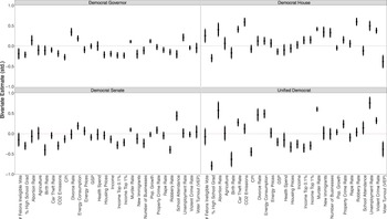
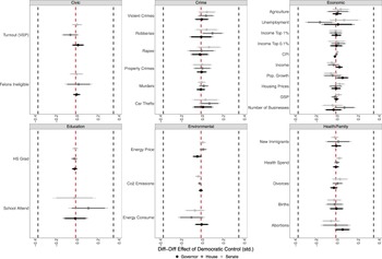
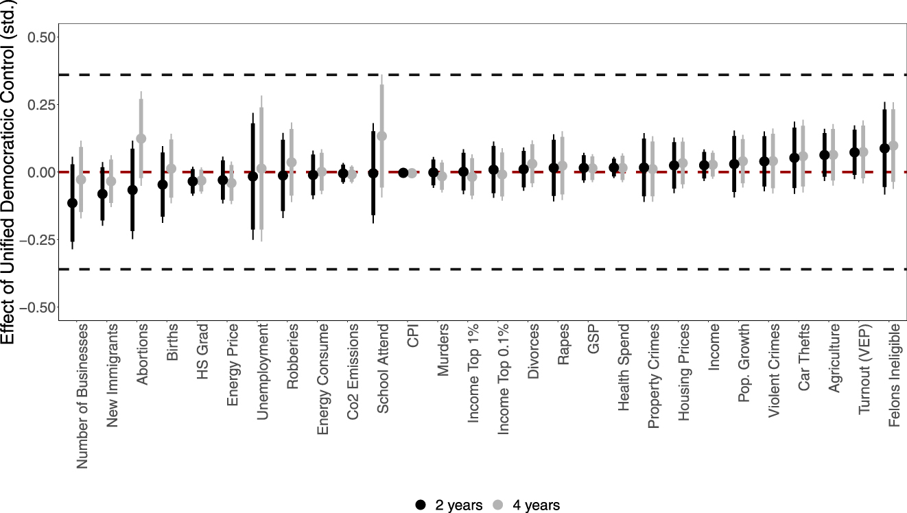
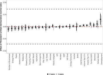
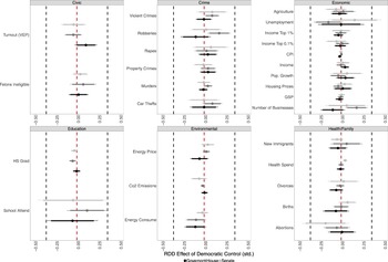
Comments

No Comments have been published for this article.

Article contents

Noisy Retrospection: The Effect of Party Control on Policy Outcomes

Abstract

Information

IMPORTANCE OF STUDYING PARTY CONTROL’S EFFECTS ON OUTCOMES

Retrospective Voting on Policy Outcomes in State Politics

DOES PARTY CONTROL AFFECT OUTCOMES?

Reasons Why Party Control May Affect Outcomes

Reasons Why Party Control May Not Affect Outcomes

DATA

Bivariate Comparisons

METHODS

Supplemental Method: Regression Discontinuity Design

Statistical Precision and Multiple Hypothesis Corrections

RESULTS

Difference-in-Difference Estimates

Regression Discontinuity Estimates

DISCUSSION

SUPPLEMENTARY MATERIAL

Footnotes

References

REFERENCES

Dynes and Holbein supplementary material

Comments

Save article to Kindle

Save article to Dropbox

Save article to Google Drive

Reply to: Submit a response

Your details

You have entered the maximum number of contributors

Conflicting interests