Introduction
Zooplankton represent an important link between primary producers and higher trophic level consumers, and play a key role in the flux of nutrients and biomass in oceanic food webs. The assemblage comprises diverse taxonomic groups with complex population dynamics driven by both environmental and biological conditions. In the off-shelf (deepwater) region of the Gulf of Mexico (GOM), the zooplankton species abundances and community composition respond to the variability in hydrography, which is mostly governed by the incursion of the Loop Current (LC) into the basin (Rowe, Reference Rowe and Ward2017).
The GOM is a semi-enclosed sea linked through the LC to the Caribbean Sea and to the Atlantic Ocean. The LC enters the GOM from the Caribbean through the Yucatan Channel, looping eastward and then southward to exit the Gulf through the Strait of Florida (Tenreiro et al., Reference Tenreiro, Candela, Sanz, Sheinbaum and Ochoa2018). In its passage through the GOM, warm core anticyclonic eddies occasionally spin off the LC and travel westward until reaching the western basin several months later, where they dissipate (Fratantoni et al., Reference Fratantoni, Lee, Podesta and Müller-Karger1998; Sturges & Lugo-Fernandez, Reference Sturges and Lugo-Fernandez2005). The strong influence of the LC and its associated circulation pattern, as well as the shallowing of the mixed layer depth in summer and the low seaward influx of coastal waters off-shelf, contribute to the oligotrophic characteristics in oceanic waters of GOM (water depths >300 m, Biggs & Ressler, Reference Biggs and Ressler2001), which in turn results in low standing stocks of plankton biomass (Müller-Karger et al., Reference Müller-Karger, Walsh, Evans and Meyers1991, Reference Müller-Karger, Smith, Werner, Chen, Roffer, Liu, Muhling, Lindo-Atichati, Lamkin, Cerdeira-Estrada and Enfield2015; Linacre et al., Reference Linacre, Lara-Lara, Camacho-Ibar, Herguera, Bazán-Guzmán and Ferreira-Bartrina2015; Rowe, Reference Rowe and Ward2017). However, cyclonic eddies and frontal transition zones associated with the shedding of anticyclonic gyres may enhance planktonic productivity through shoaling of the nitracline (Biggs & Muller-Karger, Reference Biggs and Muller-Karger1994; Biggs et al., Reference Biggs, Zimmerman, Gasca, Suárez-Morales, Castellanos-Osorio and Leben1997; Wells et al., Reference Wells, Rooker, Quigg and Wissel2017). High productivity in the deep sector of the GOM is similarly related to the semi-permanent cyclonic eddy confined to the south-west of the Bay of Campeche (BC), and to the confluence of seasonal along-coast currents that induces offshore cross-shelf transport of chlorophyll-rich waters (Martínez-López & Zavala-Hidalgo, Reference Martínez-López and Zavala-Hidalgo2009). Overall, the high variability in appearance and persistence of mesoscale features in the GOM, as well as the periodic occurrence of freshwater runoff from major rivers, may result in locally enriched patches of enhanced algal productivity and zooplankton biomass (Wormuth et al., Reference Wormuth, Ressler, Cady and Harris2000; Biggs & Ressler, Reference Biggs and Ressler2001; Okolodkov, Reference Okolodkov2003; Callejas-Jimenez et al., Reference Callejas-Jimenez, Santamaría-Del-Ángel, Gonzalez-Silvera, Millan-Nuñez and Cajal-Medrano2012; Müller-Karger et al., Reference Müller-Karger, Smith, Werner, Chen, Roffer, Liu, Muhling, Lindo-Atichati, Lamkin, Cerdeira-Estrada and Enfield2015; Rowe, Reference Rowe and Ward2017; Wells et al., Reference Wells, Rooker, Quigg and Wissel2017; Färber Lorda et al., Reference Färber Lorda, Athié, Camacho Ibar, Daessle and Molina2019).
Studies of the relationships between the abundance of different zooplankton groups and the mesoscale features have few precedents in oceanic sectors of the GOM. Overall, the warm-core less productive anticyclonic gyres sustain lower abundance and zooplankton biomass than the surrounding oceanic waters and cyclonic gyres (Biggs, Reference Biggs1992). Cyclonic gyres are generally more productive and sustain zooplankton communities with higher total abundance, albeit differing species composition (Biggs et al., Reference Biggs, Zimmerman, Gasca, Suárez-Morales, Castellanos-Osorio and Leben1997; Castellanos-Osorio & Gasca, Reference Castellanos-Osorio and Gasca1999; Wormuth et al., Reference Wormuth, Ressler, Cady and Harris2000; Gasca, Reference Gasca2003a, Reference Gasca2003b). Furthermore, differences in species composition of zooplankton between cyclonic or anticyclonic gyres and upwelling areas can vary seasonally and may be obscured by daily vertical migration (Hopkins, Reference Hopkins1982; Castellanos-Osorio & Gasca, Reference Castellanos-Osorio and Gasca1999; Wormuth et al., Reference Wormuth, Ressler, Cady and Harris2000; Gasca et al., Reference Gasca, Manzanilla and Suárez-Morales2009).
The zooplankton assemblage of the deep basins of the GOM is dominated in both abundance and biomass by calanoid copepods followed by euphausiids and chaetognaths (Hopkins, Reference Hopkins1982; Suárez-Morales et al., Reference Suárez-Morales, Fleeger, Montagna, Tunnell, Felder and Earle2009; Rowe, Reference Rowe and Ward2017). However, some low-abundance taxa, such as cnidarians and pelagic tunicates, bloom under favourable conditions and may occasionally dominate the zooplankton (Esnal, Reference Esnal1979; Suarez-Morales et al., Reference Suarez-Morales, Gasca, Segura-Puertas and Biggs2002; Flores-Coto et al., Reference Flores-Coto, Sanvicente-Añorve, Vázquez-Gutiérrez and Sánchez-Ramírez2010; Sanvicente-Añorve et al., Reference Sanvicente-Añorve, Lemus-Santana, Flores-Coto and Alatorre-Mendieta2013; Martell-Hernández et al., Reference Martell-Hernández, Sánchez-Ramírez and Ocaña-Luna2014; Färber Lorda et al., Reference Färber Lorda, Athié, Camacho Ibar, Daessle and Molina2019). These blooms are frequently associated with the occurrence of other diverse taxa (Schabetsberger et al., Reference Schabetsberger, Morgan, Brodeur, Potts, Peterson and Emmett2003; Gasca et al., Reference Gasca, Manzanilla and Suárez-Morales2009). In the GOM, for example, hyperiid amphipod aggregations have been related to mesoscale dynamics (Gasca, Reference Gasca2003b) but also to pelagic cnidarian assemblages (Gasca et al., Reference Gasca, Manzanilla and Suárez-Morales2009), highlighting the role that biological associations play in the composition and abundance of the zooplankton community.
Besides cnidarians, the abundance of hyperiid amphipods is also associated during some life history stages with other gelatinous organisms including salps, doliolids and pyrosomes. The relationships between amphipods and pelagic tunicates may be commensal (e.g. providing shelter) or parasitic (Madin & Harbison, Reference Madin and Harbison1977; Laval, Reference Laval1980). The close association between tunicates and amphipods partly explained their distribution and abundance in other ocean regions strongly influenced by mesoscale features (Lavaniegos & Ohman, Reference Lavaniegos, Ohman, Schram and von V. Klein1999; Lavaniegos & Hereu, Reference Lavaniegos and Hereu2009; Valencia & Giraldo, Reference Valencia and Giraldo2012), but no previous study explored the relationship in the abundance of these two taxa in the GOM. Few studies have focused on salp occurrence in this basin, however Esnal (Reference Esnal1979) highlighted the presence of dense aggregations of salps in the Bank of Campeche and the coasts of the Yucatan Peninsula which she associated with the high productivity in those areas (Esnal, Reference Esnal1979; Hereu & Suárez-Morales, Reference Hereu and Suárez-Morales2012). In this study we characterize the zooplankton assemblages and their relationship to hydrographic conditions along N–S transects covering deep-water regions of the southern GOM (<26°N) during two summers (2015 and 2016), with particular focus on salps and hyperiid amphipods. North–south transects cover the oceanic region of the central Gulf of Mexico that is highly influenced by LC-eddy dynamics, to the more productive Bay of Campeche dominated by the semi-permanent cyclonic gyre and cross-shelf transport during the autumn. We present evidence supporting the hypothesis that patterns of zooplankton species composition and abundance are determined both by the hydrographic conditions (especially water column stratification) and by the ecological associations among species including the symbiotic relationship between salps and amphipods.
Materials and methods
Hydrographic and biological sampling
Hydrography
Samples were collected during two oceanographic research cruises in the deep basin sector (depth >400 m) of the southern GOM (20–25°N 87–95°W; Figure 1). The cruises were carried out on board RV ‘Justo Sierra’ from 27 August to 16 September 2015 (XIXIMI–4) and from 10–24 June 2016 (XIXIMI–5). At each station, continuous measurements of temperature (SBE3 Plus), conductivity (SBE 4C), dissolved oxygen (SBE 43) and chlorophyll fluorescence (WETLabs–ECO–FLRTD) were made from the surface to 1000 m or the bottom with a CTD/rosette. Data from sensors were processed with SBE Data Processing software (Seasoft V2 software suite, 2013; http://www.seabird.com/). The base of the mixed layer (MLD) was defined as the depth at which the temperature differed from that at 10 m by >0.5°C (Kara et al., Reference Kara, Rochford and Hurlburt2000). Sea surface height (SSH) overlying kinetic and vorticity isosurface maps were used to characterize the prevailing circulation pattern during both cruises. The altimetry maps were derived from AVISO Ssalto/DUACS L4, V1.0, Grid Series products processed as described by Dominguez-Guadarrama & Pérez-Brunius (Reference Dominguez-Guadarrama and Pérez-Brunius2017).
(A) The study area in the southern Gulf of Mexico (GOM); (B) sampling grid during XIXIMI cruises (XIXIMI–4: August–September 2015 and XIXIMI–5: June 2016). Selected stations for zooplankton analysis are shown with stars. Eight stations were covered in the Yucatan Channel (YC) only during XIXIMI–4 cruise, located along two parallel lines A (north) and B (south) (named in offshore direction Y1A, Y1B to Y4A, Y4B); (C) stations covering north–south: transect 1, stations A2 to H46; transect 2, stations A3 to H48 and transect 3, A10 to Y2 (XIXIMI–4) and B37 to B18 (XIXIMI–5). BC, Bay of Campeche. Sampling time at selected stations is denoted by a white star (day) and black star (night). Left symbol for XIXIMI–4 and right symbol for XIXIMI–5.

Zooplankton sampling
Stations were selected from the sampling grid corresponding to each cruise, that included 46 and 35 stations for XIXIMI–4 and XIXIMI–5, respectively. From the sampling grid, 10 stations were selected from each cruise to analyse the composition of the zooplankton assemblage. Nine stations were located along two north–south transects plus another station located close to the Loop Current mesoscale feature (stations A2 to H48, Figure 1). The selection of stations followed these criteria: they should be located in a somewhat north–south transect within the southern GOM and they should share the same location in both cruises. Additionally, eight stations that were covered in Yucatan Channel (YC) during XIXIMI–4 were only analysed to evaluate the zooplankton community structure of source waters (Loop Current) to the GOM. The YC stations were sampled along two close parallel lines located perpendicular to the coastline. Standardized oblique net hauls were done with Bongo nets (333 mm mesh) from 200 m to the surface. Samples were preserved in 99% undenatured ethyl alcohol for metagenomic analysis. In the laboratory, samples were split using a Folsom splitter and 1/4 to 1/8 splits (Supplementary Table S1) and used for identification of major groups of organisms (excluding fish eggs and larvae, and protist) using a Zeiss stereomicroscope (Stemi 305). Hyperiid amphipods and salps from the same subsamples (excluding stations at YC) were identified to the lowest possible taxonomic level with the aid of specialized keys (Harbison & Madin, Reference Harbison and Madin1976; Vinogradov et al., Reference Vinogradov, Volkov, Semenova and Causey1996; Esnal & Daponte, Reference Esnal, Daponte and Boltovskoy1999; Zeidler, Reference Zeidler2016).
Data analysis
The main oceanographic variables were visualized in contour plots generated with Ocean Data View software (Schlitzer, Reference Schlitzer2018). Vertical distribution (0–300 m) of hydrographic parameters were plotted at the selected stations along meridional transects. Some measured and derived variables (see below) were related to biological variables (zooplankton abundance and species composition) in further analysis. Abundance was estimated as the number of organisms/1000 m3 for major taxonomic groups and for selected species (salps and amphipods). Abundance data were log10(x + 1) transformed previous to multivariate analysis.
Zooplankton taxonomic groups that comprised >0.5% were selected for multivariate analysis, which represented 15 out of 26 major taxonomic groups (Supplementary Table S2). We evaluated the temporal and spatial patterns of variation in zooplankton composition for the 15 taxonomic groups at the Phylum to Order level; species-level analysis was possible for salps and hyperiid amphipods. Previous to the multivariate analysis, we tested for potential abundance differences in total zooplankton and in five of the dominant taxa between day and night samples. A hierarchical classification of stations by log-transformed zooplankton abundance was performed by UPGMA (Unweighted Pair Group Method with Arithmetic mean) using the Bray–Curtis dissimilarity matrix. The clustering of stations and groups was complemented by an ordination technique using NMDS (Non-metric Multidimensional Scaling) based on the Bray–Curtis dissimilarity matrix, and assessed through the stress value. The resulting ordinations were two dimensions, which had an acceptable stress (<0.2) (Borcard et al., Reference Borcard, Gillet and Legendre2018). The hierarchical classification was performed with function hclust from cluster package (Maechler et al., Reference Maechler, Rousseeuw, Struyf, Hubert and Hornik2017), while ordination was obtained with the metaMDS function from vegan package in R (Oksanen et al., Reference Oksanen, Blanchet, Friendly, Kindt, Legendre, McGlinn, Minchin, O'Hara, Simpson, Solymos, Stevens, Szoecs and Wagner2018). The relationships between plankton community structure and environmental variables (temperature, salinity, oxygen and fluorescence, averaged for 0–200 m), MLD and depth of 15°C isotherm (as indicator of mesoscale features, Biggs et al., Reference Biggs, Zimmerman, Gasca, Suárez-Morales, Castellanos-Osorio and Leben1997) were assessed with the envfit function in the vegan package. This function calculates the correlation and direction of forcing of the selected environmental variables to unconstrained ordination, in order to help with interpretation in the NMDS space. The significance of the correlation was assessed using 999 random permutations of the environmental variables. The differences in zooplankton assemblages between groups of samples were tested using an ANOSIM routine.
Spearman rank correlation analysis was performed to explore the possible relationship between abundances of amphipods and their gelatinous hosts. The Spearman correlation index was also obtained in pair-wise comparison of co-occurring salp and hyperiid species. The Bonferroni correction was applied according to the number of comparisons k (α’ = α/k).
Results
Environmental conditions
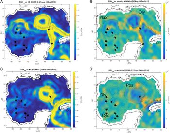
Prevailing conditions and circulation patterns during Summer 2015 and 2016 are described based on profiles of hydrographic variables and maps of sea surface height (SSH). In both years, the influence of the Loop Current (LC) is evident to the north-east of the Yucatan peninsula, however the SSH data showed a more pronounced incursion of the LC into the north-western GOM during August–September 2015 (Figure 2A, B). The presence of two large anticyclonic gyres is denoted by the negative vorticity values north of stations A7–A10 in 2015 (Figure 2C) and near stations A8–A10 in 2016 (Figure 2D); the LC-derived anticyclones were named ‘Olympus’ and ‘Poseidon’ (https://www.horizonmarine.com/loop-current-eddies). Similarly, in the north-western extent of the sampling area (~95°W) another anticyclonic gyre, known as ‘Nautilus 2’, was observed approaching the coast in 2015 (Figure 2A, B), and the remnant of ‘Olympus’ was also present in 2016 (Figure 2C, D). Smaller cyclonic and anticyclonic eddies of lesser intensity were detected in the southern sector of the GOM, and there was a more pronounced cyclonic vorticity in the south-west of the Bay of Campeche (BC; ~20°N/95°W) during June 2016 (Figure 2D). This feature has been observed repeatedly in that region (Pérez-Brunius et al., Reference Pérez-Brunius, García-Carrillo, Dubranna, Sheinbaum and Candela2013; Linacre et al., Reference Linacre, Lara-Lara, Camacho-Ibar, Herguera, Bazán-Guzmán and Ferreira-Bartrina2015).
Maps of the altimetry (SSH contours), kinetic energy (KE) and vorticity in the Gulf of Mexico. (A–B) XIXIMI–4 (August–September 2015); (C–D) XIXIMI–5 (June 2016). Data derived from AVISO products (http://www.aviso.altimetry.fr/duacs/) were provided by Dominguez-Guadarrama & Pérez-Brunius (Reference Dominguez-Guadarrama and Pérez-Brunius2017). Anticyclonic gyres abbreviations are for ‘Olympus’ (Oly), ‘Poseidon’ (Pos) and ‘Nautilus 2’ (Na2). Location of a semi-permanent cyclonic gyre (Cyc) is also shown.

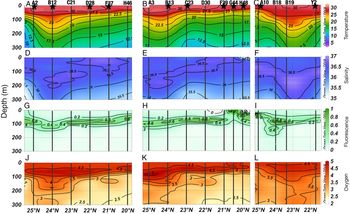
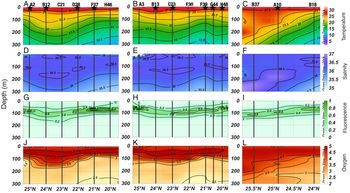
The circulation pattern observed at the surface is also reflected in the profiles of environmental variables in the upper layers, primarily for temperature, oxygen and fluorescence (chlorophyll) (Figures 3 & 4). Additionally, the depth of the 15°C isotherm denotes the areas under the influence of mesoscale eddies, with uplifted isotherms in cyclonic eddies at the southern stations, and deepened isotherms in anticyclonic eddies at northern stations (Figure 5). During both years, warm (>20°C) water was observed at 200 m depth, accompanied by a deepening of the fluorescence maximum (Figures 3 & 4). A shallowing of those features was observed at southern stations, but more pronounced around stations X4-G44 – H48 along transect 2 in 2015 (XIXIMI–4) where a stronger influence of the Grijalva–Usumacinta rivers discharge was observed, evidenced by the lower surface salinity. Around station X5-F37, along transect 1 in 2016 (XIXIMI–5), shoaling was due to the proximity of a more pronounced semi-permanent cyclone in the south-western BC.
Hydrographic conditions of water column (0–300 m) along meridional transect 1 (left), transect 2 (middle) and transect 3 (right) covered during summer 2015 XIXIMI–4 cruise. (A–C) temperature (°C); (D–F) salinity (PSU); (G–I) fluorescence (relative units) and, (J–L) oxygen (ml l−1). Station numbers and sites where zooplankton was collected (stars) are indicated in top panels.

Hydrographic conditions of water column (0–300 m) along meridional transects 1 (left), transect 2 (middle) and transect 3 (right) covered during summer 2016 XIXIMI–5 cruise. (A–C) temperature (°C); (D–F) salinity (PSU); (G–I) fluorescence (relative units) and, (J–L) oxygen (ml l−1). Station numbers and sites where zooplankton was collected (stars) are indicated in top panels.

Depth of the 15°C isotherm during summer 2015 XIXIMI–4 (August–September 2015) and summer XIXIMI–5 (June 2016). Dots indicate position of selected stations for the analysis of zooplankton community structure.

Zooplankton composition and abundance
Zooplankton abundance varied between 2015 and 2016 cruises and along transects. During summer 2015, average total abundance was higher in the deep basin of GOM (192,686 ind./1000 m3) and lower in Yucatan Channel (YC; 62,333 ind./1000 m3). Average total zooplankton abundance in central and southern regions was lower during summer 2016 (96,486 ind./1000 m3) than the previous summer (Figure 6A, D). These patterns of abundance resulted primarily from variations in copepod abundances (Figure 6B, E) which accounted for an average 55% (Stations YC) and 58% of the total abundance in 2015 and 68% in 2016 (interior GOM stations) (Figure 7). Peaks of abundance occurred at southern stations in the BC in 2015, while abundance was distributed more homogeneously in 2016. There were no differences between day and night samples for total zooplankton abundance nor for dominant taxa (Supplementary Figure S2).
Standardized abundance of zooplankton (left), copepods (centre) and non-copepod taxa (right) at select stations covered during summer 2015 (XIXIMI–4) and summer 2016 (XIXIMI–5). Colours represent day (grey) and night (black) samples. The 1000, 2000 and 3000 m isobaths are shown.

Average relative abundance of main zooplankton groups during each cruise/region. X4–YC and X4–GOM are the stations covered in the Yucatan Channel and the Gulf basin during August–September 2015 (XIXIMI–4), respectively, and X5–GOM are stations covered within the Gulf in June 2016 (XIXIMI–5).

The grouping of stations according to the 15 most abundant groups of zooplankton is represented in an ordination plot (Figure 8). The NMDS showed three main groups of stations sampled from each region during each cruise, however clusters were only weakly structured (Average Silhouette Width = 0.2). Most of the stations sampled during Summer 2015 clustered in one group (except station X4-B12), and the remaining stations formed two other separate subgroups, one containing most of Summer 2016 stations and one YC station (X4-Y1A), and the other containing the YC stations plus two that were located within anticyclones (X4-B12 and X5-A10). While most abundant zooplankton groups were present during both Summer 2015 and 2016 (Supplementary Figure S1), some taxonomic groups differed in abundance (log-transformed) between years and helped to explain the grouping of samples. Clustering was explained mainly by larvae of gastropods, echinoderms and bryozoans, as well as adults of chaetognaths, amphipods and pelagic tunicates (appendicularians, salps and doliolids). Overall, the clustering of samples based on the primary groups of zooplankton reflected differences in abundance between both years and regions, especially the interior of the Gulf vs stations from the YC. The regression analysis of select environmental variables to ordination axes was significant (P < 0.05) for four of the six variables, including average water column temperature and salinity, and the depth of the 15°C isotherm, with higher values in 2015 at stations in the YC under the influence of the Loop Current (Table 1; Supplementary Table S3). Average fluorescence was higher during 2016. The grouping of stations may be related to the observed mesoscale features (i.e. cyclones and LC). This grouping of stations included a cluster with most of YC stations (under LC influence), stations X5-A10 and X4-B12 influenced by anticyclone gyres (Figures 2 & 8), and another distinct cluster with stations G44 and H48 influenced by BC in both years.
(A) Grouping of stations according to a cluster analysis using the Bray–Curtis dissimilarity index; (B) Non-metric multidimensional scaling analysis of zooplankton of most abundant groups. Dotted lines enclose stations within distinct clusters. Stations names (in A) and symbol (in B) according to cruise/region. YC: Yucatan Channel. Arrows point in the direction of the correlation with environmental variables (shown in black if correlations are significant at P < 0. 05). Abreviations for averaged (0–200 m) environmental variables are: temperature (T_aver), salinity (S_aver), oxygen (O_aver), fluorescence (F_aver); mixed layer depth (MLD) and depth of the 15°C isotherm (D15). Abbreviations for zooplankton are: Amphipoda (AmpA), Apendicularia (ApenA), Chaetognatha (ChaeA), Copepoda (CopA), Decapoda (DecA), Doliolida (DoliA), Euphausiacea (EuphA), Echinodermata larvae (LequiA), Bryozoa larvae (LbryA), Ostracoda (OstrA), Other Gastropoda (OgasA), Polychaeta (PolA), Pteropoda (PterA), Salpida (SalpA) and Siphonophora (SiphA).

Correlation among environmental variables and ordination axis

Average (0–200 m) values for temperature, salinity, oxygen and fluorescence (RU, relative units). MLD is for mixed layer depth and D15, for depth of the 15°C isotherm. Significant correlations are indicated by a P value in italics.
Composition and abundance of salps and amphipods
Salps and amphipods comprised a small proportion of total zooplankton abundance (<3%), however they helped to explain the differences in planktonic communities between years. The average total abundance of amphipods was 2202 (± 2829) ind./1000 m3 in 2015 and 722 (± 358) ind./1000 m3 in 2016, while salps showed a similar variation pattern, with 1807 (± 2927) ind./1000 m3 and 305 (± 213) ind./1000 m3, respectively (Figure 9). However, pairwise comparisons based on Wilcoxon–Mann–Whitney U-tests showed that only salp abundance was significantly higher in 2015 (XIXIMI–4) than in 2016 (XIXIMI–5) (W = 89.5, P = 0.003) while abundance of hyperiids did not differ between years (W = 69, P = 0.159). No significant differences between day–night samples were observed for total abundance of either taxon (Supplementary Figure S3).
Abundance of hyperiid amphipods (A, C) and salps (B, D) during XIXIMI–4 (summer 2015, A, B) and XIXIMI–5 (summer 2016, C–D) cruises. Colours indicate day (grey) and night (black) samples. The 1000, 2000 and 3000 m isobaths are shown.

A total of 56 species of amphipods was identified in samples from the 20 stations (Table 2). Some individuals were identified only to genus or family level, many of them corresponded to juveniles of Primno spp. Ten species of salps were identified in samples from both cruises; two taxa were identified to genus, and a group of aggregates belonging to the genus Thalia could not be assigned to a species, particularly after preservation in alcohol. A total of 26 amphipod and 6 salp species were collected during both 2015 and 2016, while 14 species of amphipods and 2 species of salps were found only during the first summer; and 16 amphipod and 3 salp species were collected only during 2016. The dominant taxa differed between years, with Lestrigonus bengalensis Giles, 1887 ranking first in 2015 (mean abundance = 1161 ind./1000 m3, relative abundance 53%) and fifth in 2016 (21 ind./1000 m3), while Anchilomera blossevillei Milne-Edwards, 1830 (mean abundance = 96 ind./1000 m3; relative abundance 13%) ranked first in adult abundance. If juveniles of Primno spp. are considered (127 ind./1000 m3, 18% of total amphipod abundance), A. blossevillei ranked second. Among salps, Ilhea punctata (Forskål, 1775) was dominant in 2015 due to a bloom in one station (abundance = 7946 ind./1000 m3; 44% of total salp abundance), followed by Iasys cylindrica (Cuvier, 1804) (mean abundance 346 ind./1000 m3; 19% of total salp abundance). Iasys cylindrica ranked first the following summer (mean abundance 108 ind./1000 m3; 35% of total salp abundance).
Average abundance and total abundance (TA) (individuals/1000 m3), standard deviation (SD), and relative abundance (%RA) for hyperiid amphipods and salps during summers of 2015 and 2016 in the deep-water region of the Gulf of Mexico

The most abundant species (average abundance ranking 1 to 5) are indicated in bold. Abbrev. column indicates abbreviation of species name.
The ANOSIM analysis showed that amphipod and salp abundances differed significantly between years (R = 0.2444, P = 0.002). The SIMPER analysis indicated that 13 hyperiid and 2 salp species were mostly (65%) responsible for dissimilarities between years, including primarily the most abundant species collected in each cruise (Table 3). Cluster analysis and ordinations for communities were analysed for each year separately. For amphipods and salps collected in 2015, grouping resulting from the Bray–Curtis cluster analysis assembled most of the central-southern stations (Figure 10A, B), while station B12 (within the anticyclone Nautilus II) and station A10 (close to the Loop Current) clustered separately. The spatial configuration of sample groups in the non-metric multidimensional scaling (NMDS) analysis was consistent with the clustering results, with higher similarity of more closely located stations. Station B12 had high abundance of Thalia spp., Eupronoe minuta Claus, 1879 and Traustedtia multitentaculata (Quoy & Gaimard, 1834), whereas the eastern station A10 was rich in Primno spp. juveniles. Those species together with L. bengalensis, I. cylindrica, Phronimopsis spiniphera Claus, 1879 and Brachyscelus crusculum Spence Bate, 1861 contributed the most to the dissimilarities between these stations and those located in the southern basin of GOM. The patterns of variation of environmental variables during Summer 2015 showed no significant relationship to patterns for zooplankton communities, based on the regression analysis. For Summer 2016, the cluster analysis revealed that station A10 was distinct from the remaining stations, which clustered into two groups, in which northern (A2 to C23) and southern (D28 to H48) stations grouped together. Primno evansi Sheader, 1986, Primno juveniles, A. blossevillei, P. spinifera, Phrosina semilunata Risso, 1822 and Thalia spp., were the primary drivers (Figure 11B). Station A10, which was located in the anticyclonic gyre, had overall low amphipod and salp abundances (abundance = 132 ind./1000 m3 for both groups) and species richness; this station was characterized by the presence of Platyscelus ovoides (Risso, 1816), and moderate abundances of I. cylindrica and Thalia spp. Four environmental variables were significantly correlated with the zooplankton ordination axes (Figure 11B).
(A) Grouping of stations based on a cluster analysis of salp and amphipod log transformed abundance for the XIXIMI–4 cruise (summer 2015) based on the Bray–Curtis distance; (B) Non-metric multidimensional scaling analysis on salp and amphipod log transformed abundance. Colour of symbols indicate day (grey) and night (black) samples. Arrows point in the direction of the correlation with environmental variables (none of the correlations were significant at P < 0. 05). Species name code in Table 2. Abbreviations for environmental variables same as in Figure 8.

(A) Grouping of stations based on a cluster analysis of salp and amphipod log transformed abundance for the XIXIMI–5 cruise (summer 2016) based on the Bray–Curtis distance; (B) Non-metric multidimensional scaling analysis on salp and amphipod log transformed abundance. Colour of symbols indicate day (grey) and night (black) samples. Arrows point in the direction of the correlation with environmental variables (shown in black if correlations are significant at P < 0.05). Species name code in Table 2. Abbreviations for environmental variables as in Figure 8.

SIMPER analysis discriminating species of salps and hyperiid amphipods between summer cruises using Bray–Curtis dissimilarities

Summer 2015 (XIXIMI–4); summer 2016 (XIXIMI–5). Av. Dissim: average dissimilarities among cruises; Av. abundance: average abundance re-calculated from log transformed abundances; Contr%: percentage contribution of each species to average dissimilarities; Cum.%: cumulative percentage (shown up to 65%)
The Spearman rank correlation of amphipods and their possible gelatinous host abundances revealed positive correlations with salps, doliolids and cnidarians (mainly siphonophores), but the correlation was higher and significant only for salps (ρ = 0.48, P < 0.031) (Table 4a). There were positive correlations among five salp and six amphipod species (ρ > 0.45, P < 0.05; Table 4b). Additionally, an abundance peak in the salp I. punctata observed in 2015 corresponded with a peak in L. bengalensis, the most abundant amphipod.
(a) Spearman rank correlation (rho) and probabilities among amphipods and possible gelatinous hosts; (b) Correlations among species pairs of most frequent amphipods and salps

a Siphonophores + Medusae.

a Thalia spp. is for T. cicar, T. democratica and T. orientalis solitary and aggregates zooids.
Discussion
Zooplankton community structure and environmental variables
The hydrographic conditions in the central Gulf of Mexico during Summer 2015 and 2016 were under the influence of the mesoscale features frequently occurring within this basin, denoted mainly by the presence of two large anticyclonic eddies. Anticyclonic circulation was identifiable by deepening of isolines of temperature, salinity, dissolved oxygen and chlorophyll maxima at stations in central GOM, contrasting with the BC, where uplifted isolines are indicative of cyclonic circulation in both years (Biggs, Reference Biggs1992; Biggs et al., Reference Biggs, Zimmerman, Gasca, Suárez-Morales, Castellanos-Osorio and Leben1997; Okolodkov, Reference Okolodkov2003; Pérez-Brunius et al., Reference Pérez-Brunius, García-Carrillo, Dubranna, Sheinbaum and Candela2013; Linacre et al., Reference Linacre, Lara-Lara, Camacho-Ibar, Herguera, Bazán-Guzmán and Ferreira-Bartrina2015). Although similar mesoscale circulation was observed during both cruises, the results of the multivariate analyses point to differences in total abundance as well as in the relative proportions of the less abundant groups. These differences are likely linked to seasonal environmental differences, particularly to a warmer and deeper mixed layer in August–September 2015 that is more typical of late summer–autumn (Pasqueron De Fommervault et al., Reference Pasqueron De Fommervault, Pérez-Brunius, Damien, Camacho-Ibar and Sheinbaum2017), while the lower temperature observed in the upper water column in June 2016 is more consistent with the spring–summer transition period.
Seasonality in zooplankton standing stocks is better documented than total zooplankton abundance in the deep basins of the GOM. Most studies have indicated an overall increase in biomass during summer (Wormuth et al., Reference Wormuth, Ressler, Cady and Harris2000; Zavala-García et al., Reference Zavala-García, Flores-Coto and de la Luz Espinosa-Fuentes2016; Färber Lorda et al., Reference Färber Lorda, Athié, Camacho Ibar, Daessle and Molina2019), which is consistent with the observed pattern of a higher total zooplankton abundance during the late summer 2015 cruise, compared with the early summer cruise in 2016. The discharge of nutrient-rich waters from major rivers onto the continental shelf of the southern GOM that occurs during the rainy season (June–October), as well as seasonal coastal-offshore transport strongly influences the zooplankton abundance and distribution resulting in an enhanced zooplankton biomass (Okolodkov, Reference Okolodkov2003; de la Luz Espinosa-Fuentes et al., Reference de la Luz Espinosa-Fuentes, Flores-Coto, Sanvicente-Añorve and Zavala-García2009; Zavala-García et al., Reference Zavala-García, Flores-Coto and de la Luz Espinosa-Fuentes2016; Färber Lorda et al., Reference Färber Lorda, Athié, Camacho Ibar, Daessle and Molina2019). In their multi-annual study, Zavala-García et al. (Reference Zavala-García, Flores-Coto and de la Luz Espinosa-Fuentes2016) described higher zooplankton biomass to be consistently observed during summer in a strong relationship to the intensification of continental water discharged into the ocean between July and December at the southern BC, which we also observed at southern BC during August–September 2015. The influence of water discharge during this period was evidenced by the lower salinity values at the surface and the shallower peak in fluorescence values in the southernmost station (station X4-H48) of transect 2. Additionally, high plankton productivity in the Bank of Campeche and adjacent shelf break can result from coastal upwelling (Salas-de-León et al., Reference Salas-de-León, Monreal-Gómez, Signoret and Aldeco2004; Zavala-García et al., Reference Zavala-García, Flores-Coto and de la Luz Espinosa-Fuentes2016; Gomez et al., Reference Gómez, Lee, Hernández, Chiaverano, Müller-Karger, Liu and Lamkin2019). This process could explain the high zooplankton abundance at station X4-G44, which is located just off the western Yucatan platform, and associated changes in the temperature and fluorescence profiles. Also, the shallower fluorescence observed at X4-G44 was accompanied by a higher fluorescence value compared with stations in the central Gulf. Higher fluorescence may indicate higher chlorophyll, which can result in population increases of several taxa, e.g. doliolids and salps, which are known to form blooms in response to sudden peaks in chlorophyll concentrations on the shelf (Deibel & Paffenhöfer, Reference Deibel and Paffenhöfer2009). Similarly, in the southern BC region Färber-Lorda et al. (Reference Färber Lorda, Athié, Camacho Ibar, Daessle and Molina2019) reported higher zooplankton biomass in the summer of 2011 (research cruise XIXIMI–2), driven by extensive blooms of salps, in clear association with heavy precipitation during that season. In this study, conditions promoting higher plankton stocks (i.e. upwelling and the presence of lower salinity water near the surface indicative of freshwater discharge and offshore transport) were not evident during June 2016, and we documented a moderate and more homogeneous zooplankton abundance and distribution (about 4.5 times less than in 2015). This result highlights the importance of local upwelling and river transport in driving the community structure in the southern BC.
Stations within the LC at Yucatan Channel showed the influence of conditions typical of the Caribbean region, characterized by warmer waters and low plankton biomass (Okolodkov, Reference Okolodkov2003; Carrillo et al., Reference Carrillo, Johns, Smith, Lamkin and Largier2016). In contrast to stations of the interior of the GOM, YC stations had higher average temperature, salinity, dissolved oxygen content and a deeper 15°C isotherm, and relatively lower zooplankton densities. Station A10, located at the edge of the meandering LC (Figure 3), had higher zooplankton abundance, which may be related to its proximity to a front. Frontal regions between counter-paired (cyclone-anticyclone) eddies or at the periphery of the anticyclonic intrusion of the warm LC have been described as areas of enhanced productivity able to sustain higher phytoplankton and zooplankton stocks relative to more oligotrophic surrounding waters or at the centre of an anticyclonic feature (Eden et al., Reference Eden, Steinberg, Goldthwait and McGillicuddy2009; Linacre et al., Reference Linacre, Lara-Lara, Camacho-Ibar, Herguera, Bazán-Guzmán and Ferreira-Bartrina2015). Station A10 was likely more influenced by the developing anticyclonic eddy in 2016 (Figure 4), and zooplankton abundance was correspondingly lowest.
The dominant zooplankton groups reported here are consistent with previous studies of the GOM (Hopkins, Reference Hopkins1982; Ortner et al., Reference Ortner, Hill and Cummings1989) and other tropical-subtropical ocean regions, where only a few taxa comprise a high percentage of the total abundance, and the remaining groups represent a small proportion (<3%) or are present at only a few stations (Landry et al., Reference Landry, Decima, Simmons, Hannides and Daniels2008; Eden et al., Reference Eden, Steinberg, Goldthwait and McGillicuddy2009; Ambriz-Arreola et al., Reference Ambriz-Arreola, Gómez-Gutiérrez, del Franco-Gordo, Plascencia-Palomera, Gasca, Kozak and Lavaniegos2018). Copepods dominated numerically in all samples, with relative abundances ranging between 46–74% of the total, followed by bryozoans in summer of 2015 and by chaetognaths during June 2016. Other dominant groups were siphonophores, ostracods, pteropods and euphausiids, and to a lesser degree decapods, amphipods, thaliaceans and larvaceans. All these taxa co-occurred in most of the samples, and the less abundant groups drove differences among groups of stations in multivariate analyses. For example, a higher proportion of larvae (of bryozoans, polychaetes and gastropods), as well as salps and amphipods explained the differences in community structure between samples collected in 2015 and 2016, particularly at YC stations. Higher proportions of larval forms have been reported during summer and autumn for different sectors of the GOM as a result of higher reproductive activity (Hopkins, Reference Hopkins1982; Gasca et al., Reference Gasca, Castellanos-Osorio and Biggs2001; Elliott et al., Reference Elliott, Pierson and Roman2012; Rowe, Reference Rowe and Ward2017; Daudén-Bengoa et al., Reference Daudén-Bengoa, Jiménez-Rosenberg, Compaire, del Pilar Echeverri-García, Pérez-Brunius and Herzka2020). Additionally, the dominance of larvae in YC is not surprising, since the east coast of the Yucatan Peninsula has a narrow continental shelf with extensive and productive reef zones, from which larval stages of benthic fauna may be transported by the dominant northward Yucatan Current into the GOM interior (Suárez-Morales & Arriaga, Reference Suárez-Morales and Arriaga1998; Álvarez-Cadena et al., Reference Álvarez-Cadena, Ordóñez-López, Almaral-Mendivil and Uicab-Sabido2009). Furthermore, the prevalence of bryozoan and gastropod larvae at several stations in 2015 suggests that mesoscale features may be acting as a dispersal mechanism for some taxa in the GOM. Similarly, Daudén-Bengoa (Reference Daudén-Bengoa, Jiménez-Rosenberg, Compaire, del Pilar Echeverri-García, Pérez-Brunius and Herzka2017) found similarities in the fish larval assemblages between YC stations and stations in the region of influence of the LC and in anticyclonic eddies.
The proportional increase in chaetognaths during June 2016 may be a response to a higher abundance of potential prey species. During this cruise, copepods were relatively more abundant than during the previous summer, which may have resulted in increased abundance of their predators, such as chaetognaths and siphonophores, which ranked second and third in abundance, respectively. Similarly, Gasca & Suárez (Reference Gasca and Suárez1991) related increased densities of siphonophores in the Bank of Campeche area to the abundance of herbivore populations.
Composition and abundance of hyperiid amphipod and salp assemblages
The hyperiid amphipods identified in the samples at the southern Gulf of Mexico represented 56% of the species known to occur within the basin, while salp species represented 59% of the species reported for the gulf (LeCroy et al., Reference LeCroy, Gasca, Winfield, Ortíz, Escobar-Briones, Tunnell, Felder and Earle2009; Hereu & Suárez-Morales, Reference Hereu and Suárez-Morales2012). Previous reports from two summer cruises in the southern GOM by Gasca (Reference Gasca2004) and Gasca et al. (Reference Gasca, Manzanilla and Suárez-Morales2009) reported 71 and 57 hyperiid amphipods; they sampled over a comparable area but analysed more stations (97 and 57, respectively) including neritic stations that were not covered in this study. Similarly to what is reported in this study, Esnal (Reference Esnal1979) registered eight species of salps from more than 30 stations within the gulf. The relatively high number of species registered in our 10 oceanic stations (41–42 hyperiids and 8–9 salps) is consistent with the oceanic affinity and distribution patterns of both taxa; abundances tend to be lower and diversity higher in open ocean rather than neritic regions (<200 m depth) (Esnal, Reference Esnal1979; Gasca, Reference Gasca2003a; Deibel & Paffenhöfer, Reference Deibel and Paffenhöfer2009; Gasca et al., Reference Gasca, Manzanilla and Suárez-Morales2009). Since we analysed only a subset of zooplankton samples collected during summer 2015 and 2016, it is likely that actual diversity during both periods and throughout the region was higher, and additional species might be identified, particularly during night-time collections. Several epipelagic and mesopelagic amphipods and salps are known to perform extensive vertical migrations, moving into the surface layer during the night and descending during daylight hours to depths below 200 m (Vinogradov et al., Reference Vinogradov, Volkov, Semenova and Causey1996; Andersen, Reference Andersen and Bone1998; Gasca, Reference Gasca2007, Reference Gasca2009). For example, an average of 4 salp species were collected in night-time samples, compared with an average of 2 during the day. Salpa fusiformis and S. maxima, known as large diel migrators (Andersen, Reference Andersen and Bone1998) were exclusively present in night collections. For hyperiid amphipods the averages were 10 species for night-time samples and 8 for daytime samples during 2015, while in 2016 the opposite was observed (averages were 8 and 10 species for night and day samples, respectively). However, mean differences between day and night species and abundances were not significant for both taxa (P > 0.34 for all comparisons). Furthermore, some individuals could only be assigned to genus (Brachyscelus sp., Eupronoe sp. and Primno sp.) or family (Lycaeidae) levels (all of them known to dwell in epipelagic to mesopelagic waters; LeCroy et al., Reference LeCroy, Gasca, Winfield, Ortíz, Escobar-Briones, Tunnell, Felder and Earle2009), so differences between day and night species abundances and richness between both periods may occur.
Compared with other taxa, total salp and amphipod abundances were moderate, but similar to, values reported within the GOM and other oligotrophic areas (Madin & Deibel, Reference Madin, Deibel and Bone1998; Gasca, Reference Gasca2007; Gasca et al., Reference Gasca, Manzanilla and Suárez-Morales2009; Hereu et al., Reference Hereu, Lavaniegos and Goericke2010), following a spatial distribution pattern similar to that of total zooplankton. Average densities for both groups differed between years, with higher numbers during 2015 (XIXIMI–4), but differences were more pronounced (and significant) for salps (average abundance was 6 times higher than in 2016) than for amphipods (average abundance was 3 times higher). The pattern in salps and amphipods abundance during summer 2015 and 2016 are consistent with those observed for samples collected in previous XIXIMI–1 to XIXIMI–3 cruises (autumn 2010, summer 2011 and winter 2013, respectively). Herzka et al. (Reference Herzka, Herguera, Licea, Sheinbaum, Ferreira, Camacho, Díaz, Farber, García, Ayón, Huerta, Lara-Lara, Lares, Lizárraga, Macías, Millán, Riquelme and Rocha2014) reported summer average abundances of 924 and 2197 ind./1000 m3 for hyperiid amphipods and salps, respectively (XIXIMI–2). Autumn (XIXIMI–1) average abundances were 532 and 376 ind./1000 m3, respectively, and 1034 and 0 ind./1000 m3 for winter (XIXIMI–3). Similarly, Gasca et al. (Reference Gasca, Manzanilla and Suárez-Morales2009) reported high variability in hyperiid amphipod abundances, with lower values in spring 1986 (average 875 ind./1000 m3) than summer 1988 (average 1437 ind./1000 m3), but also a lower average abundance in summer (411 ind./1000 m3) compared with winter (1376 ind./1000 m3) of the same year. A high seasonality in the abundances of both taxa is evident, although it is more marked in salps, probably related to their ability to bloom and to take advantage of favourable conditions (i.e. sudden productivity pulses). The variability in hyperiid amphipod abundance may be coupled not only to salps but also to other gelatinous hosts, such as cnidarians, which are relatively abundant and consistently present in the GOM (Gasca, Reference Gasca1999; Gasca et al., Reference Gasca, Manzanilla and Suárez-Morales2009; Sanvicente-Añorve et al., Reference Sanvicente-Añorve, Alba, Flores-Coto and Castillo-Rivera2009).
The high average total abundance we report for the summer of 2015 was influenced partly by the salp bloom found at station X4-G44, next to the Bank of Campeche. As previously noted, this station is in an upwelling favourable region (Salas-de-León et al., Reference Salas-de-León, Monreal-Gómez, Signoret and Aldeco2004), which may have resulted in high food availability for opportunistic filter feeders such as doliolids (ranking third in abundance at the station) and the salps Ihlea punctata and Thalia democratica (Forskål, 1775) (Esnal, Reference Esnal1979; Deibel & Paffenhöfer, Reference Deibel and Paffenhöfer2009). These blooms may have favoured the presence of the hyperiid Lestrigonius bengalensis, the dominant amphipod at that station (84% numerical abundance). This species is the most common hyperiid in neritic waters in the GOM (Stuck et al., Reference Stuck, Perry and Fish1980; Gasca, Reference Gasca2003a) and high abundances have been previously reported at the north-western border of the Yucatan shelf in summer in association with pelagic cnidarians (Gasca et al., Reference Gasca, Manzanilla and Suárez-Morales2009). To our knowledge, there are no previous reports of the massive occurrence of I. punctata, but similar blooms have been reported for two congeneric species (Daponte et al., Reference Daponte, Calcagno, Acevedo-Luque, Martos, Machinandiarena and Esnal2011; Pakhomov et al., Reference Pakhomov, Dubischar, Hunt, Strass, Cisewski, Siegel, von Harbou, Gurney, Kitchener and Bathmann2011), and its relationship to L. bengalensis is not clear. However, association between the salps I. punctata and T. democratica with the hyperiids Vibilia armata Bovallius, 1887, V. propincua Stebbing, 1888 and Phronima sedentaria (Forskål, 1775) has been reported (summarized in Laval, Reference Laval1980) so a facultative relationship between L. bengalensis and co-occurring salps is possible.
The dominant species we identified during both cruises were similar to those previously reported for the tropical north-western Atlantic and for the GOM (Esnal, Reference Esnal1979; Stuck et al., Reference Stuck, Perry and Fish1980; Gasca, Reference Gasca2007; Gasca et al., Reference Gasca, Manzanilla and Suárez-Morales2009; Hereu & Suárez-Morales, Reference Hereu and Suárez-Morales2012; Burridge et al., Reference Burridge, Tump, Vonk, Goetze and Peijnenburg2017). Several studies have highlighted the dominance of L. bengalensis in the southern GOM during spring, summer and winter (Gasca, Reference Gasca2004; Gasca et al., Reference Gasca, Manzanilla and Suárez-Morales2009). However, those studies sampled high proportions of neritic stations, where this species thrives, and lower to moderate abundances are usually found at more oceanic stations. In our samples, L. bengalensis and species in the genus Primno (including the juveniles) were among the most abundant during both years, in agreement with Gasca (Reference Gasca2004), who described higher reproductive activity for both species during summer when compared with spring. Nevertheless, while in summer of 2015 the amphipod L. bengalensis ranked first (53% RA, Table 2), followed by Primno species (8%), Phronimopsis spinifera (7%) and Phrosina semilunata (2%), the former species ranked sixth (RA 3%) in summer of 2016, while Primno group (mainly juveniles) and Ancylomera blossevillei dominated (25% and 13% of relative abundance), followed by Brachyscelus globiceps and Hyperietta stephenseni Bowman, 1973 (RA 5% each). The difference in abundance and dominance pattern among both periods points to the marked seasonality of the amphipods community structure in oceanic waters of the southern GOM, with a considerable portion of variability driven by the performance of the dominant species, L. bengalensis, as well as the abundance of gelatinous hosts, such as salps and cnidarians.
The dominant salp species, Iasys cylindrica and Thalia spp. (T. cicar Van Soest, 1973, T. democratica and T. orientalis Tokioka, 1937) have also been reported as conspicuous in tropical and subtropical waters as well as in the southern GOM and Caribbean sea. They were also reported as blooming species in strong association with highly productive areas (Esnal, Reference Esnal1979; Deibel & Paffenhöfer, Reference Deibel and Paffenhöfer2009). In this study, the abundance of Iasys cylindrica was only surpassed by Ihlea punctata, which was only found blooming at station G44 in 2015. The remaining species have also been reported in the area although less frequently and in markedly lower abundances. Salpa fusiformis Cuvier, 1804 was scarcely present and Salpa maxima Forskål, 1775, recently registered as a new record for the western Caribbean Sea (Hereu & Suárez-Morales, Reference Hereu and Suárez-Morales2012), is reported here within GOM waters for the first time.
Salp, hyperiid amphipods and environmental variables
Marked mesoscale variations in salps and hyperiid amphipod abundance and species composition may be expected due to the presence of cyclonic and anticyclonic gyres in the oceanic waters of the GOM. Besides seasonal differences in zooplankton community composition, the groupings of stations resulting from multivariate analysis (Figures 10 & 11) are consistent with the broad environmental characteristics that prevail in the oceanic regions of the GOM. Thus, in both summers, a similar spatial distribution emerged, where stations located to the north (~22°N) tended to cluster and were distinct from those to the south, suggesting the existence of common environmental features within those regions and some homogeneity in their epipelagic assemblages. Characteristics of the salp and amphipod assemblages in those sectors are similar to those depicted for other taxa (Gasca, Reference Gasca1999; Gasca et al., Reference Gasca, Castellanos-Osorio and Biggs2001; Suárez-Morales et al., Reference Suarez-Morales, Gasca, Segura-Puertas and Biggs2002; Daudén-Bengoa, Reference Daudén-Bengoa, Jiménez-Rosenberg, Compaire, del Pilar Echeverri-García, Pérez-Brunius and Herzka2017) where stations in anticyclonic LC eddies characterized by a warmer upper layer tended to sustain lower abundances and fewer species than southern stations associated with cyclonic circulation. Similar studies that characterized the oceanic sector of the GOM also differentiated the Bay of Campeche from the sector immediately north to the bay. For example, Okolodkov (Reference Okolodkov2003) divided the area encompassed by the XIXIMI sampling grid into two distinctive regions based on productivity: lower productivity in the central GOM, a region influenced by LC anticyclonic eddies, and higher productivity in the southern sector related to the predominant cyclonic circulation and off-shelf transports. A similar partitioning of the GOM open waters was described by Damien et al. (Reference Damien, Pasqueron de Fommervault, Sheinbaum, Jouanno, Camacho-Ibar and Duteil2018) according to modelled integrated chlorophyll content (0–350 m layer). In this study, stations within well-developed mesoscale features (like station B12 located within the ‘Nautilus 2’ anticyclone during XIXIMI–4 and station A10 at the ‘Poseidon’ anticyclone XIXIMI–5) showed the lowest diversity and abundance, consistent with low productivity and downwelling. These eddies had detached from the LC about 2.5 months (B12) and 1.5 months (A10) before the sampling period, so the community was probably not mixed with those of surrounding ‘gulf’ waters.
Salps and hyperiid amphipods correlations
The distribution of hyperiid amphipods can be associated in great part to distribution of their gelatinous hosts (Laval, Reference Laval1980; Lavaniegos & Ohman, Reference Lavaniegos, Ohman, Schram and von V. Klein1999; Gasca et al., Reference Gasca, Suárez-Morales and Haddock2007, Reference Gasca, Manzanilla and Suárez-Morales2009; Valencia & Giraldo, Reference Valencia and Giraldo2012). Although symbiotic relationships are better described based on direct observations, possible associations can be inferred from co-occurrences in net collections, particularly when abundance of both symbionts is high. The positive correlations we found between pairs of species may represent true symbiotic associations, since they have been well described in the literature for some of the species listed in Table 4. As mentioned earlier, the occurrence of the highest abundances for Lestrigonus bengalensis and Ihlea punctata at X4-G44 is remarkable, and may reflect a symbiotic relationship. This amphipod has been described as a symbiont of the medusa Eirene pyramidalis (Agassiz, 1862) (Harbison et al., Reference Harbison, Biggs and Madin1977) and the siphonophore Diphyes bojani (Eschscholtz, 1825) (de Lima & Valentin, Reference de Lima and Valentin2001), but the latter authors also found it inside the salp Thalia democratica in most of the stations where the species was collected. This salp species was particularly abundant at the station where L. bengalensis was also abundant, so a symbiotic association among both species within GOM waters is likely. Since summer is the main reproductive season for L. bengalensis (Gasca, Reference Gasca2004), salps may be acting as their host during this period. Several Vibilia species have an obligate relationship with salps, so a relationship with Traustedtia multitentaculata can be expected. The hyperiids Brachyscelus and Eupronoe have also been associated with Cyclosalpa as a host (Madin & Harbison, Reference Madin and Harbison1977; Laval, Reference Laval1980). Anchylomera blossevillei have been related to pyrosomes, another colonial pelagic tunicate. According to Bowman (Reference Bowman1978), the host may be used as shelter to deposit the amphipod's larvae, in a similar way as Vibilia does with salps. Probably, the relationship among amphipods and salps during summer corresponds more to the reproductive activity of the former group during this season. The consistent presence of juvenile forms in the samples supports this proposition.
Conclusions
This study showed differences in zooplankton communities between two consecutive summers. Differences in zooplankton communities are seen not only in total abundance, but also in terms of the relative contribution of various taxonomic groups, with larval forms occurring in greater abundances during late summer. Spatial differences in the zooplankton assemblage were linked to the hydrological characteristics associated with mesoscale features. Zooplankton abundance was generally low in northern regions under the influence of anticyclonic gyres, while stations in the BC showed higher zooplankton abundance, likely as a result of enhanced productivity driven by freshwater discharge and upwelling. Salp and hyperiid amphipod assemblages were also related to mesoscale features, with lower species richness and abundances in stations associated with LC anticyclonic eddies. Only a few species dominated the salp community during the summer, when productivity peaks drove bloom formations in the GOM. The pattern and timing of hyperiid amphipod peak abundances was more variable and most probably driven by seasonal changes in reproduction of the dominant species, and symbiotic associations with salp species.
Supplementary material
The supplementary material for this article can be found at https://doi.org/10.1017/S0025315420000715
Acknowledgements
We are grateful to Dr Ann Bucklin for her valuable suggestions to the manuscript. We thank the Captain and crew of the Buque Oceanográfico Justo Sierra (UNAM).
Financial support
This research was funded by the National Council of Science and Technology of Mexico – Mexican Ministry of Energy – Hydrocarbon Trust, project 201441. This is a contribution of the Gulf of Mexico Research Consortium (CIGoM).