1. Introduction
Understanding the behaviour of non-Brownian suspension flows is of primary importance in many biological systems and engineering applications. Many experimental, theoretical and numerical works have been devoted to this purpose in the past. We refer to recent reviews for details (Denn & Morris Reference Denn and Morris2014; Guazzelli & Pouliquen Reference Guazzelli and Pouliquen2018; Morris Reference Morris2020b, Reference Morris2023; Lemaire et al. Reference Lemaire, Blanc, Claudet, Gallier, Lobry and Peters2023). In the first place, the slow behaviour of non-Brownian suspension in homogeneous shear flow (HSF) is now well documented. Shear stress as well as normal stress differences have been measured in experiments and numerical simulations. The corresponding material functions, i.e. relative shear viscosity and normal stress differences, diverge as the jamming volume fraction  $\phi _J$ is approached. The shear-induced microstructure is of great importance in this matter, as shown in shear reversal experiments and simulations (Gadala-Maria & Acrivos Reference Gadala-Maria and Acrivos1980; Blanc, Peters & Lemaire Reference Blanc, Peters and Lemaire2011; Lin et al. Reference Lin, Guy, Hermes, Ness, Sun, Poon and Cohen2015; Peters et al. Reference Peters, Ghigliotti, Gallier, Blanc, Lemaire and Lobry2016), with subtle effects in shear-rotation experiments (Blanc et al. Reference Blanc, Peters, Gillissen, Cates, Bosio, Benarroche and Mari2023). We note that the difficult matter of extensional flows has received much less attention in experiments (Dai & Tanner Reference Dai and Tanner2017), simulations (Seto, Giusteri & Martiniello Reference Seto, Giusteri and Martiniello2017; Cheal & Ness Reference Cheal and Ness2018) and theory (Jenkins, Seto & La Ragione Reference Jenkins, Seto and La Ragione2021).
In the last two decades, the idea that contact forces between particles play a primary role has emerged. Friction between particles is now known to strongly increase the shear viscosity (Seto et al. Reference Seto, Mari, Morris and Denn2013; Gallier et al. Reference Gallier, Lemaire, Peters and Lobry2014b), mainly by decreasing the jamming volume fraction (Singh et al. Reference Singh, Mari, Denn and Morris2018; Chèvremont, Chareyre & Bodiguel Reference Chèvremont, Chareyre and Bodiguel2019; Lobry et al. Reference Lobry, Lemaire, Blanc, Gallier and Peters2019; Peerbooms et al. Reference Peerbooms, Nadorp, van der Heijden and Breugem2024). As the volume fraction approaches  $\phi _J$, the contribution of the contact forces to the shear stress is increasingly predominant. This idea has been very fruitful in explaining the shear-thickening behaviour of non-Brownian suspensions by a lubricated-to-frictional transition (Mari et al. Reference Mari, Seto, Morris and Denn2014; Morris Reference Morris2020a). It has also been shown that the shear-thinning behaviour of frictional suspensions observed in experiments could be explained by the decrease of the friction coefficient with increasing interparticle forces (Chatté et al. Reference Chatté, Comtet, Nigues, Bocquet, Siria, Ducouret, Lequeux, Lenoir, Ovarlez and Colin2018; Lobry et al. Reference Lobry, Lemaire, Blanc, Gallier and Peters2019; Arshad et al. Reference Arshad, Maali, Claudet, Lobry, Peters and Lemaire2021; Le et al. Reference Le, Izzet, Ovarlez and Colin2023; Lemaire et al. Reference Lemaire, Blanc, Claudet, Gallier, Lobry and Peters2023).
Similarly, suspension pressure, and more generally normal stresses, bear both hydrodynamic and contact origin. In a sheared suspension, the repulsive contacts, which keep the particles from overlapping, induce a positive pressure in the material, tending to dilate the particle network, while the (negative) pressure in the suspending liquid – the pore pressure – resists this dilation, as experiments in rheometric flows have shown (Deboeuf et al. Reference Deboeuf, Gauthier, Martin, Yurkovetsky and Morris2009; Dbouk, Lobry & Lemaire Reference Dbouk, Lobry and Lemaire2013; Garland et al. Reference Garland, Gauthier, Martin and Morris2013). This concept is also connected to the Reynolds dilatancy of very concentrated immersed granular materials, which must dilate to flow, inducing the same negative fluid pressure, with important implications on the transient starting flow, for instance in the collapse of a granular column (Rondon, Pouliquen & Aussillous Reference Rondon, Pouliquen and Aussillous2011) or even in simple shear flow (Marzougui, Chareyre & Chauchat Reference Marzougui, Chareyre and Chauchat2015; Athani et al. Reference Athani, Metzger, Forterre and Mari2022). In the field of suspension rheology, this concept has been promoted by pressure-controlled experiments, where particle pressure is controlled instead of volume fraction, allowing us to probe highly concentrated suspensions, popularizing a new formulation of the material functions from the dry granular community: the  $\mu$-rheology (Boyer, Guazzelli & Pouliquen Reference Boyer, Guazzelli and Pouliquen2011). The latter has also proved to be fruitful in experiments on shear-thickening suspensions (Clavaud, Metzger & Forterre Reference Clavaud, Metzger and Forterre2020; Etcheverry, Forterre & Metzger Reference Etcheverry, Forterre and Metzger2023).
In heterogeneous flows, where volume fraction or shear rate are not uniform, particle migration is observed (Guazzelli & Pouliquen Reference Guazzelli and Pouliquen2018; Morris Reference Morris2023). Such a behaviour has been evidenced for a long time in cylindrical Couette flow (Leighton & Acrivos Reference Leighton and Acrivos1987; Abbott et al. Reference Abbott, Tetlow, Graham, Altobelli, Fukushima, Mondy and Stephens1991). In such a case, particles migrate towards the external wall, where the shear rate and shear stress are lower. In pressure-driven flows, particles migrate towards the centre of the tube, where both shear rate and shear stress vanish (Koh, Hookham & Leal Reference Koh, Hookham and Leal1994; Hampton et al. Reference Hampton, Mammoli, Graham, Tetlow and Altobelli1997; Lyon & Leal Reference Lyon and Leal1998). As shear-induced migration had been evidenced, a phenomenological model was proposed, based on diffusion fluxes linearly related to volume fraction and shear rate gradients (Leighton & Acrivos Reference Leighton and Acrivos1987; Phillips et al. Reference Phillips, Armstrong, Brown, Graham and Abbott1992). This model, which can account for dense particle viscous resuspension as well (Leighton & Acrivos Reference Leighton and Acrivos1986), has benefited from refinements (Krishnan, Beimfohr & Leighton Reference Krishnan, Beimfohr and Leighton1996), in particular, to account for particle segregation (Shauly, Wachs & Nir Reference Shauly, Wachs and Nir1998; Chun et al. Reference Chun, Park, Jung and Won2019).
Nott & Brady (Reference Nott and Brady1994) introduced the suspension balance model (SBM) in their attempt to get a deeper insight into migration, with particular attention to their Stokesian Dynamics simulations of a pressure-driven flow. Starting from the fundamental pointwise momentum balance equation inside the particles, they derive the particle phase momentum equation, according to which the migration flux is induced by the gradient of the particle pressure. Accounting for normal stress anisotropy, Morris & Boulay (Reference Morris and Boulay1999) generalized the model to curvilinear geometries, thereby allowing prediction of particle migration in the main rheometric flows. Later, Lhuillier (Reference Lhuillier2009) and Nott, Guazzelli & Pouliquen (Reference Nott, Guazzelli and Pouliquen2011) investigated the importance of the various contributions to the particle stress and the hydrodynamic forces involved in particle transport. The contact force contribution to the particle stress was identified as the primary driving force for particle migration, with still open questions concerning supplementary hydrodynamic contributions. Differently phrased, the interphase force, i.e. the average fluid force applied to the particle phase, is assumed to be a drag force, proportional to the difference between particle phase and suspension velocities, with possible supplementary contributions though. This will be recalled in § 3. We note that the SBM has also been recently extended to bidisperse suspensions (Howard, Maxey & Gallier Reference Howard, Maxey and Gallier2022).
The SBM predictions have been compared with experimental measurements, mostly in steady flow after the migration is complete, in the main shear flows used in rheological studies (Morris & Boulay Reference Morris and Boulay1999; Miller & Morris Reference Miller and Morris2006; Snook, Butler & Guazzelli Reference Snook, Butler and Guazzelli2016; Rashedi et al. Reference Rashedi, Sarabian, Firouznia, Roberts, Ovarlez and Hormozi2020). The comparison involves the volume fraction and velocity profiles and requires the constitutive laws for both suspension and particle stresses. The agreement is generally good, except for the centreline of pressure-driven flows, where the shear rate vanishes. In that position, the SBM predicts that the jamming volume fraction is reached, no matter how small the initial volume fraction is, which is not observed in experiments. Modifications of the stress constitutive laws have been proposed, to account for non-local effects (Nott & Brady Reference Nott and Brady1994; Mills & Snabre Reference Mills and Snabre1995; Miller & Morris Reference Miller and Morris2006), resulting in finite normal stress at the centreline and a better agreement with experiments (Mills & Snabre Reference Mills and Snabre1995; Miller & Morris Reference Miller and Morris2006). Such non-local laws are physically sound, in particular, given that the ratio of the system size to the particle size is usually not very large – often a few tens – in experiments and simulations.
Prediction of the transient profiles requires the hindered settling function as measured in sedimentation experiments. They are conveniently predicted in wide-gap Couette flow (Morris & Boulay Reference Morris and Boulay1999), but the agreement seems less good in pressure-driven flow (Snook et al. Reference Snook, Butler and Guazzelli2016; Rashedi et al. Reference Rashedi, Sarabian, Firouznia, Roberts, Ovarlez and Hormozi2020), or at the cost of a significant modification of the hindered settling function (Miller & Morris Reference Miller and Morris2006).
We note here that the SBM requires precise knowledge of the stress constitutive laws and of the hindered settling function to yield velocity and volume fraction profiles in transient and steady flow. In particular, particle normal stresses are not easily measured in experiments (Zarraga, Hill & Leighton Reference Zarraga, Hill and Leighton2000; Boyer et al. Reference Boyer, Guazzelli and Pouliquen2011; Dbouk et al. Reference Dbouk, Lobry and Lemaire2013), and variations are expected due to different contact behaviours (Lobry et al. Reference Lobry, Lemaire, Blanc, Gallier and Peters2019; Clavaud et al. Reference Clavaud, Metzger and Forterre2020). As a consequence, the corresponding constitutive laws are not always available for interpretation of migration experiments (Miller & Morris Reference Miller and Morris2006; Snook et al. Reference Snook, Butler and Guazzelli2016; Rashedi et al. Reference Rashedi, Sarabian, Firouznia, Roberts, Ovarlez and Hormozi2020).
From this perspective, particle-resolved simulations are of primary interest, since they yield precise knowledge of all relevant quantities at the local scale, including the various stresses. Among the simple rheometric flows, the pressure-driven channel flow is very attractive, due to its simplicity and relatively low computational cost. It is, therefore, no surprise that most of the simulation studies devoted to particle migration deal with channel flows (Nott & Brady Reference Nott and Brady1994; Yeo & Maxey Reference Yeo and Maxey2011; Chun et al. Reference Chun, Kwon, Jung and Hyun2017, Reference Chun, Park, Jung and Won2019; Di Vaira et al. Reference Di Vaira, Łaniewski-Wołłk, Johnson, Aminossadati and Leonardi2022; Howard et al. Reference Howard, Maxey and Gallier2022, Reference Howard, Dong, Patel, D'Elia, Maxey and Stinis2023), sometimes considering finite inertia (Hogendoorn et al. Reference Hogendoorn, Breugem, Frank, Bruschewski, Grundmann and Poelma2023), or with the conceptually close case of the Kolmogorov flow (Gillissen & Ness Reference Gillissen and Ness2020; Bhowmik & Ness Reference Bhowmik and Ness2024). Other studies have considered the influence of gravity, for instance in bed-load transport (Vowinckel et al. Reference Vowinckel, Biegert, Meiburg, Aussillous and Guazzelli2021), or inertia (Shajahan et al. Reference Shajahan, Schouten, Raaghav, van Rhee, Keetels and Breugem2024).
In the specific case of channel flows, Nott & Brady (Reference Nott and Brady1994) defined ad hoc plausible functions to model the normal stresses, including non-local contribution, and compared their data from Stokesian dynamics simulations of frictionless particles with computations of steady flow from the SBM. Morris & Brady (Reference Morris and Brady1998) followed the same approach in a channel flow of dense suspensions, where gravity acts in a direction perpendicular to the channel. Yeo & Maxey (Reference Yeo and Maxey2011) performed simulations of a channel flow using the force coupling method (FCM) corrected for lubrication interactions, again with frictionless particles. They computed particle stress profiles in steady flow once the migration was completed. They divided the channel into three regions: a wall region near the boundaries; a core region in the channel centre; and an intermediate region. The transverse normal stress – in the velocity gradient direction – in the intermediate region was found to be relatively uniform, consistent with the predictions of the SBM, and the particle pressure was in good agreement with the constitutive law proposed by Morris & Boulay (Reference Morris and Boulay1999). In addition, the viscosity from the shear stress profile in the intermediate region was found to be well described by standard correlation laws. It should also be noted that they found, for sufficiently low mean volume fraction  $\bar {\phi } \leq 0.3$, that the volume fraction at the centre did not reach the jamming volume fraction, in agreement with experiments from the literature. In a recent paper, Howard et al. (Reference Howard, Dong, Patel, D'Elia, Maxey and Stinis2023) used their data from particle-resolved simulations (i.e. FCM) of the channel flow of monodisperse and bidisperse frictionless suspensions at mean volume fraction
 $\bar {\phi }=0.4$ to feed both physics-informed machine learning and data-informed operator learning, to predict the development of the particle stress in the suspension as migration occurs. They observe a good agreement for the monodisperse suspension between the transient particle flux as measured in the simulations and as computed from the transient stress using the SBM.
Finally, Gillissen & Ness (Reference Gillissen and Ness2020) studied concentrated frictional suspensions in heterogeneous flows using the discrete element method in two dimensions. They focused on the constitutive law for the mean stress. To explain their simulation data, they adapted a recent model based on a time-varying structure tensor (Gillissen et al. Reference Gillissen, Ness, Peterson, Wilson and Cates2019), allowing the strain rate tensor fluctuations to induce stresses. More specifically, at positions where the shear rate vanishes, the fluctuations, and the normal stresses as well, do not. The SBM fed with such a constitutive law predicts a steady volume fraction profile that shows over- or under-compaction ( $\max (\phi ) \gtrless \phi _J$), depending on the intensity of the fluctuations. Bhowmik & Ness (Reference Bhowmik and Ness2024) performed similar three-dimensional simulations of frictionless suspensions in the high volume fraction range
 $\phi \geq 0.5$. Their data allowed them to build constitutive laws for the stresses that would involve, in addition to the usual volume fraction, macroscopic friction coefficient, and viscous number, a supplementary dimensionless number,
 $\varTheta$, that stands for the dimensionless particle velocity fluctuations. The predicted profiles from the SBM agree well with the simulation profiles.
In the present article, we perform particle-resolved numerical simulations of non-Brownian frictional suspensions in channel flow. The purpose of this work is to extensively characterize particle migration, both in the transient dynamic regime and steady flow after the migration is complete, from a local perspective, i.e. considering local space- and time-averaged quantities, and check the main constitutive laws on which the SBM is based. As will be recalled in the following, the SBM is derived from fundamental mass and momentum balance equations, and the yielded equations must be supplemented by various constitutive laws, involving local stress gradients, particle and suspension velocities, etc. We want to primarily focus on these constitutive laws.
Before getting into this matter, other issues deserve to be addressed. For instance, since local stress gradients are involved in the considered constitutive law, the numerical method should keep the usual momentum balance equation for the locally averaged suspension stresses, which requires that the corresponding laws perfectly hold at the particle scale. This will be checked. At this point, the choice of the numerical method deserves a few words. Various efficient numerical methods are available to simulate low Reynolds number flows of particulate suspensions (see Orsi, Lobry & Peters (Reference Orsi, Lobry and Peters2023) and references therein for an account of them). In the present article, local volume fractions in the wide range [0.25, 0.65] are considered, so that, in addition to contact interactions, both long-range and lubrication hydrodynamic interactions should be properly accounted for. In the present study, we use the fictitious domain method (FDM) supplemented by subgrid (lubrication) corrections (Gallier et al. Reference Gallier, Lemaire, Lobry and Peters2014a), for which we have recently developed a new formulation of the subgrid corrections that is well suited to nonlinear flows while preserving the necessary frame-indifference (Orsi et al. Reference Orsi, Lobry and Peters2023).
In addition, the SBM equations can predict the transient and steady volume fraction and velocity profiles provided that the usual constitutive laws for the stress are given, which involve the standard material functions such as shear viscosity, normal viscosity and macroscopic friction coefficient. In the present article, we measure these laws and material functions at each point of the heterogeneous flow in the channel, and compare them with their counterpart in HSF, as measured with the same numerical method, which are also consistent with correlation laws proposed by Badia et al. (Reference Badia, D'Angelo, Peters and Lobry2022).
The main features of the FDM are recalled in § 2. Then, the SBM is shortly explained in § 3 with particular attention to the main assumptions and necessary constitutive laws, and the method used for the computation of the various locally averaged quantities is detailed in § 4. The transient and steady volume fraction and velocity profiles are investigated in § 5. The local momentum balance equation for the suspension, together with the local stress constitutive laws, are examined in § 6. Finally, the main hypotheses on which the SBM is based are investigated in § 7.
2. Numerical method
2.1. The FDM: a summary
The FDM has been detailed in the past (Gallier et al. Reference Gallier, Lemaire, Lobry and Peters2014a), including the specific version that is used in the present article (Orsi et al. Reference Orsi, Lobry and Peters2023). The main features of the method are recalled here. In the FDM, the flow of a Newtonian liquid, with dynamic viscosity  $\eta$ and density
 $\rho$, is computed in the whole meshed simulation domain
 $\mathcal {D}$ including the particles. The particles are rigid spheres with the same density as the liquid. The rigidity of the particles is enforced using a force density
 $\rho \boldsymbol{\lambda}$ that acts only in the volume of each particle
 $\mathcal {D}_p$. In the present work, inertia is neglected for both fluid and particle dynamics. As a consequence, fluid velocity
 $\boldsymbol {u}$ and pressure
 $P$ obey modified Stokes equations
 $$\begin{gather} \left.\begin{array}{c} \boldsymbol{\nabla} \boldsymbol{\cdot} \boldsymbol{\sigma} + \rho \boldsymbol{\lambda}= \boldsymbol{0},\\ \boldsymbol{\nabla} \boldsymbol{\cdot} \boldsymbol u = 0, \end{array}\right\} \end{gather}$$
 $$\begin{gather}\boldsymbol{\sigma} ={-} P\boldsymbol{\delta} + \eta ( \boldsymbol{\nabla} \boldsymbol u + \boldsymbol{\nabla} \boldsymbol u^T), \end{gather}$$
constraining the fluid inside each particle ( $\kern 1.5pt p$) to undergo rigid body motion,
 \begin{equation} \boldsymbol u(\boldsymbol x) = \boldsymbol{U}_p + \boldsymbol{\varOmega}_p\times (\boldsymbol x - \boldsymbol x_p ) \quad \text{for} \ \boldsymbol x \in \mathcal{D}_p, \end{equation}
where  $\boldsymbol {U_p}$ and
 $\boldsymbol{\varOmega} _p$ are the particle translational and rotational velocities, respectively. In addition, various boundary conditions for the pressure and the velocity may be applied, depending on the considered specific flow. They are given in § 2.3 for the channel flow of interest in the present article.
In the present article, the particles are only subjected to hydrodynamic and contact forces. Then, Newton's equations write for each particle  $(p)$,
 \begin{equation} \left.\begin{gathered} \boldsymbol{F}^h_p + \boldsymbol{F}^c_p = \boldsymbol{0},\\ \boldsymbol{T}^h_p + \boldsymbol{T}^c_p = \boldsymbol{0}, \end{gathered}\right\} \end{equation}
where  $\boldsymbol{F}^h_p$ and
 $\boldsymbol{F}^c_p$, respectively, stand for the hydrodynamic and contact forces exerted on the particle
 $(p)$, and
 $\boldsymbol{T}^h_p$ and
 $\boldsymbol{T}^c_p$ are the corresponding torques. Contact forces and torques will be briefly described in the next section. Hydrodynamic forces and torques are split into two contributions. The first part corresponds to the moments that originate in the fluid flow computed by the solver, and are hereafter denoted by
 $\boldsymbol{F}^{FDM}_p$ and
 $\boldsymbol{T}^{FDM}_p$. These are computed as follows:
 \begin{equation} \left.\begin{gathered} \boldsymbol{F}^{FDM}_p={-} \rho \int_{\mathcal{D}_p} \boldsymbol{\lambda}\, \mathrm{d}\mathcal{V},\\ \boldsymbol{T}^{FDM}_p ={-} \rho \int_{\mathcal{D}_p} (\boldsymbol x-\boldsymbol x_p )\times \boldsymbol{\lambda}\, \mathrm{d}\mathcal{V}. \end{gathered}\right\} \end{equation}
However, the solver cannot properly compute the flow between particles when their surfaces are closer than the mesh size. As a consequence, the stress moments applied to the particles must be corrected using theoretical expressions. The method we follow in the present article has been fully explained and validated by Orsi et al. (Reference Orsi, Lobry and Peters2023). The generalized particle velocity and subgrid force vectors are, respectively, denoted by  $\boldsymbol {\mathcal {U}} = ( \boldsymbol{U}_1, \boldsymbol{U}_2, \ldots, \boldsymbol{\varOmega} _1, \boldsymbol{\varOmega} _2, \ldots )$ and
 $\boldsymbol {\mathcal {F}}^{SG} = ( \boldsymbol{F}_1^{SG}, \boldsymbol{F}_2^{SG}, \ldots, \boldsymbol{T}_1^{SG}, \boldsymbol{T}_2^{SG}, \ldots )$. The latter may be computed from the former using the subgrid resistance matrix
 $\boldsymbol {\mathcal {R}}^{SG}_{\mathcal {FU}}$,
 \begin{equation} \boldsymbol{\mathcal{F}}^{SG} ={-} \boldsymbol{\mathcal{R}}^{SG}_{\mathcal{FU}} \boldsymbol{\cdot} \boldsymbol{\mathcal{U}}, \end{equation}
where the subgrid resistance matrix depends on the fluid viscosity, particle positions and radii, and it is computed pairwise as the difference between the theoretical two-particle resistance matrix and its counterpart as measured by the uncorrected FDM solver. Finally, the total hydrodynamic force and torque read
 \begin{equation} \left.\begin{gathered} \boldsymbol{F}^h_p = \boldsymbol{F}^{FDM}_p + \boldsymbol{F}^{SG}_p, \\ \boldsymbol{T}^h_p = \boldsymbol{T}^{FDM}_p + \boldsymbol{T}^{SG}_p. \end{gathered}\right\} \end{equation}
Equation (2.6) deserves several comments. First, unlike the standard subgrid corrections, no mention of the ambient velocity field is made, meaning that only the particle velocities are needed to compute the subgrid forces. Such an expression has been fully justified by Orsi et al. (Reference Orsi, Lobry and Peters2023). It stems from the fact that only lubrication flows that involve relative velocities of particle surfaces are missed by the fluid solver, and consequently have to be considered for corrections. This formulation is especially well suited to the present flow, where the velocity profile depends on the solid volume fraction profile, which evolves in time and is not given in advance. It should also be noted that the same type of corrections has to be applied for particles close to bounding walls when particle–wall interactions have to be considered (Orsi et al. Reference Orsi, Lobry and Peters2023).
Equations (2.1)–(2.6) must be solved at each time step. The unknown quantities are the pressure and velocity fields, ( $P, \boldsymbol {u}$), the force density,
 $\rho \boldsymbol{\lambda}$, and the particle velocities,
 $\boldsymbol{U}_p$ and
 $\boldsymbol{\varOmega} _p$. The main issue lies in the determination of the force density that allows proper accounting for the constraints imposed on the particles, namely particle rigidity – equation (2.3) – and particle momentum balance – (2.4) together with (2.5)–(2.7). The numerical method that is followed to solve this problem has been explained in detail by Orsi et al. (Reference Orsi, Lobry and Peters2023). In particular, it has been implemented in the frame of the OpenFOAM toolbox, which easily allows the solving of (2.1) and (2.2) using high-performance computing facilities taking advantage of the parallelization.
2.1.1. Suspension rheology: dipole moment
To compute the effective stress in a suspension of solid particles, the first moment of the hydrodynamic surface stress acting on each particle  $\boldsymbol {D}_p$ (Batchelor Reference Batchelor1970; Lhuillier Reference Lhuillier2009; Nott et al. Reference Nott, Guazzelli and Pouliquen2011) is needed,
 \begin{align} \boldsymbol{\mathsf{D}}^{FDM}_p &= \int_{\partial \mathcal{D}_p} \boldsymbol{\sigma} \boldsymbol{\cdot} \boldsymbol n \otimes (\boldsymbol x -\boldsymbol x_p)\, \mathrm{d}\mathcal{S}\nonumber\\ &={-}\rho \int_{\mathcal{D}_p} \boldsymbol{\lambda} \otimes (\boldsymbol x - \boldsymbol x_p)\, \mathrm{d}\mathcal{V} -\left(\int_{\mathcal{D}_p} P\, \mathrm{d}\mathcal{V}\right) \boldsymbol{\delta}. \end{align}
The second equality is obtained using (2.1) and (2.2) (Orsi et al. Reference Orsi, Lobry and Peters2023).
The antisymmetric part of the force dipole  $\boldsymbol {D}^{FDM}_p$ is a tensor whose components are the components of the hydrodynamic torque
 $\boldsymbol {T}_p^{FDM}$ exerted on particle
 $(p)$, while the symmetric part is usually called stresslet. The latter is split into the deviatoric stresslet
 $\boldsymbol {S}^{FDM}_p$ and the isotropic part
 $s^{FDM}_p/3\ \boldsymbol{\delta}$, where
 $s^{FDM}_p$ stands for the trace of the force dipole. As a consequence, the FDM traceless stresslet, stresslet trace and force dipole write as
 \begin{equation} \left.\begin{gathered}
\boldsymbol{\mathsf{S}}_p^{FDM}={-}\rho \int_{\mathcal{D}_p}
\left\lbrace \tfrac{1}{2}[ \boldsymbol{\lambda}
\otimes(\boldsymbol x -\boldsymbol x_p) +(\boldsymbol x
-\boldsymbol x_p) \otimes \boldsymbol{\lambda} ]
-\tfrac{1}{3}\boldsymbol{\lambda}
\boldsymbol{\cdot}(\boldsymbol x -\boldsymbol
x_p)\boldsymbol{\delta} \right\} \mathrm{d}\mathcal{V},\\
s_p^{FDM} ={-}\int_{\mathcal{D}_p}[ \rho
\boldsymbol{\lambda} \boldsymbol{\cdot}(\boldsymbol x
-\boldsymbol x_p) +3 P ]\, \mathrm{d}\mathcal{V},\\
\boldsymbol{\mathsf{D}}^{FDM}_p = \boldsymbol{\mathsf{S}}_p^{FDM}
+\dfrac{s_p^{FDM}}{3}\boldsymbol{\delta} -
\dfrac{1}{2}\boldsymbol{\epsilon} \boldsymbol{\cdot}
\boldsymbol{T}_p^{FDM}. \end{gathered}\right\}
\end{equation}
We note here that a reference has to be defined for the pressure. It has been chosen as the mean pressure over the whole simulation volume, meaning that  $\int _D P\, \mathrm {d}\mathcal {V}=0$ at each time step.
As in the case of force and torque, a subgrid correction must be added to the FDM stresslet on the particles, which is computed using specific resistance subgrid matrices (Orsi et al. Reference Orsi, Lobry and Peters2023). The total hydrodynamic traceless stresslet, stresslet trace and force dipole are then computed as
 \begin{equation} \left.\begin{gathered} \boldsymbol{\mathsf{S}}_p^{h} = \boldsymbol{S}_p^{FDM} + \boldsymbol{S}_p^{SG},\\ s_p^{h} = s_p^{FDM} + s_p^{SG},\\ \boldsymbol{\mathsf{D}}_p^{h} = \boldsymbol{D}_p^{FDM} + \boldsymbol{D}_p^{SG}. \end{gathered}\right\} \end{equation}
2.2. Contact forces
In the present article, contact forces reflect both particle roughness and friction. They are described in detail in Gallier et al. (Reference Gallier, Lemaire, Peters and Lobry2014b), Peters et al. (Reference Peters, Ghigliotti, Gallier, Blanc, Lemaire and Lobry2016) and Orsi et al. (Reference Orsi, Lobry and Peters2023), and we give here only a short account of them. Contact between particles  $(p)$ and
 $(q)$ occurs as soon as the distance between their surfaces is smaller than the roughness height
 $h_r$, resulting in elastic forces exerted by particle
 $(q)$ on particle
 $(p)$, both normal
 $(\boldsymbol {F}^{c,n}_{pq})$ and tangential
 $(\boldsymbol {F}^{c,t}_{pq})$. Sliding is triggered as soon as the tangential force reaches the value
 $\Vert \boldsymbol {F}^{c,t}_{pq} \Vert = \mu _s \Vert \boldsymbol {F}^{c,n}_{pq} \Vert$, where
 $\mu _s$ stands for the static friction coefficient. In the sliding regime, the latter relation between normal and tangential forces holds, meaning that no difference is made here between the static and dynamic friction coefficients. The contact torques on particles
 $(p)$ and
 $(q)$ read
 \begin{equation} \boldsymbol{T}^{c}_{pq} = \dfrac{a_{p}}{a_{p}+a_{q}} \boldsymbol{x}_{pq} \times \boldsymbol{F}^{c,t}_{pq} = \dfrac{a_p}{a_q}\boldsymbol{T}^{c}_{qp}, \end{equation}
where  $a_p$ and
 $a_q$ stand for the particle radii, and
 $\boldsymbol x_{pq} = \boldsymbol x_q - \boldsymbol x_p$ is the distance between the particle centres. Contact forces also induce an additional stresslet which is given for the contacting particles
 $(p)$ and
 $(q)$ by
 \begin{equation} \boldsymbol{\mathsf{S}}^{c}_{pq} = \dfrac{1}{2} \dfrac{a_{p}}{a_{p}+a_{q}} ( \boldsymbol{F}^{c}_{pq} \otimes \boldsymbol{x}_{pq} + \boldsymbol{x}_{pq} \otimes \boldsymbol{F}^{c}_{pq} ) = \dfrac{a_p}{a_q}\boldsymbol{S}^{c}_{qp}. \end{equation}
The induced contact force dipole is written for particles  $(p)$ and
 $(q)$ as follows:
 \begin{equation} \boldsymbol{\mathsf{D}}^{c}_{pq} = \boldsymbol{\mathsf{S}}^{c}_{pq} - \dfrac{1}{2}\boldsymbol{\epsilon} \boldsymbol{\cdot} \boldsymbol{T}^c_{pq} =\dfrac{a_p}{a_q}\boldsymbol{D}^{c}_{qp}, \end{equation}
where  $\boldsymbol {\epsilon }$ stands for the Levi-Civita symbol. The stresslet in (2.12) is not traceless, and its trace determines the contribution of contact forces to particle pressure. Finally, it should be noted that the same type of frictional contact force is exerted by the bounding walls on contacting particles and contributes to the particle force dipole.
2.3. Numerical set-up
We investigate three values of the mean volume fraction  $\bar {\phi } = [0.3, 0.4,0.5]$. The suspensions are bidisperse (
 $a_2 = 1.4a_1$,
 $\overline {\phi _1} = \overline {\phi _2} = \bar {\phi }/2$) to avoid crystallization. Particles and walls are frictional, with a friction coefficient
 $\mu _s= 0.5$ and roughness height
 $h_r = 0.005a_1$. The latter is a value commonly found in experiments with model spherical particles (Blanc et al. Reference Blanc, Peters and Lemaire2011; Tanner & Dai Reference Tanner and Dai2016). The particles are initially placed at random positions in the simulation cell using the same procedure as in Howard et al. (Reference Howard, Dong, Patel, D'Elia, Maxey and Stinis2023). The size of the simulation cell is
 $(L_x,\, L_y,\, L_z) = (40 a_1,\, 40 a_1,\, 20 a_1)$ (figure 1). The fluid equations are discretized on a fixed Cartesian grid with mesh size
 $0.2 a_1$. The trade-off between precision and computation speed has been discussed in Gallier et al. (Reference Gallier, Lemaire, Lobry and Peters2014a). The flow is driven by a uniform pressure gradient in the negative
 $x$ direction so that (2.1) together with (2.2) reads
 \begin{equation} \eta \Delta \boldsymbol{u} - \boldsymbol{\nabla} p - \dfrac{\mathrm{d}P_0}{\mathrm{d}\kern0.07em x}\boldsymbol{e}_x + \rho \boldsymbol{\lambda} = \boldsymbol{0}. \end{equation}
The plane boundaries normal to the  $y$ direction are rigid walls at rest, while the other boundaries are given periodic conditions, for both the pressure perturbation
 $p$ and the velocity
 $\boldsymbol {u}$. The particle distribution is made periodic along the same directions. Length, shear rate, time, velocity and stresses are made dimensionless as follows:
 \begin{equation} y^{*} = \dfrac{y}{L_{y}}, \quad \dot{\gamma}^{*} = \dfrac{\dot{\gamma}}{\overline{\dot{\gamma}}_{0}}, \quad t^{*} = \overline{\dot{\gamma}}_{0}t, \quad \boldsymbol{u}^{*} = \dfrac{\boldsymbol{u}}{\overline{\dot{\gamma}}_{0}L_{y}}, \quad \varSigma^{*} = \dfrac{\varSigma}{\eta\overline{\dot{\gamma}}_{0}}, \end{equation}
where  $\bar {\dot {\gamma }}_0$ is the mean shear rate in a pressure-driven flow of pure liquid,
 \begin{equation} \bar{\dot{\gamma}}_{0} = \dfrac{L_{y}}{4\eta}\left\vert\dfrac{\mathrm{d}P_{0}}{\mathrm{d}\kern0.07em x}\right\vert. \end{equation}
Simulation cell.
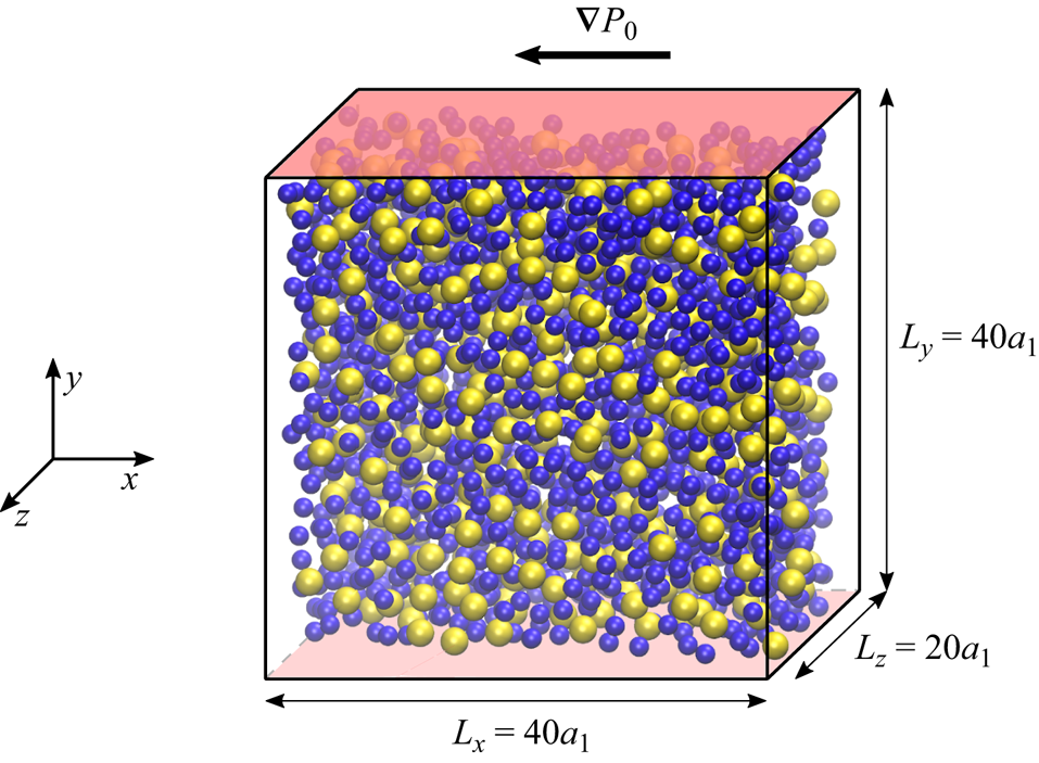
In the following, the required equations are given in dimensional form, for the sake of physical clarity. The dimensionless equations may be recovered from the dimensional ones by letting  $\eta =1$,
 $L_y=1$,
 $\bar {\dot {\gamma }}_{0}=1$, meaning for instance that
 $\mathrm {d}P_0/\mathrm {d}\kern0.07em x = -4$. However, figures display dimensionless quantities, where the superscript (*) has been dropped, though. All numerical values given in the text also correspond to dimensionless quantities.
As we will see, the actual shear rate in the channel is always lower than  $\bar {\dot {\gamma }}_{0}$ due to the enhanced viscosity induced by the particles. The time step
 $\Delta t$ – meaning
 $\bar {\dot {\gamma }}_{0}\Delta t$ – is chosen as
 $\Delta t = 2 \times 10^{-3}$ for all simulations. An estimation of the mean accumulated strain as felt by the fluid is classically computed from the mean distance covered by the fluid (Lyon & Leal Reference Lyon and Leal1998; Howard et al. Reference Howard, Maxey and Gallier2022) as
 \begin{equation} \bar \gamma(t)= \dfrac{2}{Ly}\int_0^t \left[ \dfrac{1}{V} \int_\mathcal{D} u_x\, \mathrm{d}\mathcal{V} \right] \mathrm{d}t= \dfrac{2 L_t}{Ly}. \end{equation}
The simulation parameters are gathered in table 1.
List of simulation parameters:  $\bar {\phi }$, mean volume fraction;
 $N_p$, number of particles;
 $\Delta t$, time step;
 $\bar {\gamma }_{total}$, total accumulated strain;
 $\bar {\gamma }_{steady}$, accumulated strain at steady flow start;
 $\Delta \bar {\gamma }_{steady}$, accumulated strain interval for steady averaging;
 $\Delta t_{steady}$, time interval for steady state averaging.

3. The SBM
We consider the flow of suspensions made of rigid particles suspended in an incompressible liquid. Both materials share the same density, so gravity does not play any role. No other external force is considered either, and inertia is neglected. At particle scale, besides hydrodynamic interactions, particles are supposed to interact only due to contact forces.
The SBM is based on a two-phase flow modelling of the suspension. It is derived by averaging the point balance equations valid in each material, solid and liquid, and the resulting equations involve the locally averaged volume fraction, velocities, and stresses for each phase. Various averaging methods have been proposed (Zhang & Prosperetti Reference Zhang and Prosperetti1994; Jackson Reference Jackson1997), which yield similar equations. In addition, the SBM has been recently revisited in the case of non-inertial non-Brownian suspensions (Lhuillier Reference Lhuillier2009; Nott et al. Reference Nott, Guazzelli and Pouliquen2011). Following Guazzelli & Pouliquen (Reference Guazzelli and Pouliquen2018), the main equations are briefly recalled below. Regarding the accuracy of the equations for the ratio of the particle size to the bulk flow length scale, we refer to the recent work by Ozenda (Reference Ozenda2019). A specific version of the model developed for bidisperse suspensions has been recently proposed by Howard et al. (Reference Howard, Maxey and Gallier2022). As discussed in the following sections, the radii of the particles in the present study seem sufficiently close to each other for us to consider the suspension as being monodisperse. As to the simulation data, a volume-averaging procedure is chosen, which is detailed in § 4.
Each material, solid and liquid, is incompressible, but the corresponding phases are not, due to the variation of the particle volume fraction  $\phi$. As a consequence of the constant density of particles and liquid, the mass conservation equation of each material yields the volume balance equation for each phase,
 $$\begin{gather} \dfrac{\partial \phi}{\partial t} + \boldsymbol{\nabla} \boldsymbol{\cdot}( \phi \boldsymbol{u}_p )= 0, \end{gather}$$
 $$\begin{gather}\dfrac{\partial(1-\phi)}{\partial t} + \boldsymbol{\nabla} \boldsymbol{\cdot}((1-\phi) \boldsymbol{u}_f )= 0, \end{gather}$$
where  $\boldsymbol {u}_p$ and
 $\boldsymbol {u}_f$, respectively, stand for the velocity of the particle and fluid phase. The suspension volume balance equation follows from (3.1) and (3.2), reflecting the overall incompressibility of the suspension:
 $$\begin{gather} \boldsymbol{u}_s = \phi \boldsymbol{u}_p + (1 - \phi) \boldsymbol{u}_f , \end{gather}$$
 $$\begin{gather}\boldsymbol{\nabla} \boldsymbol{\cdot} \boldsymbol{u}_s = 0. \end{gather}$$
Averaging the point momentum balance equation over each phase, solid or liquid, yields the corresponding phase momentum balance equation. In the solid phase, the following equation is obtained:
 \begin{equation} \boldsymbol{\nabla} \boldsymbol{\cdot} \boldsymbol{\varSigma}^c + n \langle\,\boldsymbol{f}^h \rangle _p = \boldsymbol{0}, \end{equation}
where  $n \langle \boldsymbol {f}^h \rangle _p$ is the interphase hydrodynamic force, i.e. the density of hydrodynamic force exerted on the particles, and
 $\boldsymbol{\varSigma} ^c$ is the particle phase stress, which is induced by contact forces between particles. It is computed as a density of force dipole moment,
 \begin{equation} \boldsymbol{\varSigma}^c = n\langle\boldsymbol{\mathsf{D}}^c \rangle _p. \end{equation}
It is worth noting that the contact stress is related to the contact force density exerted on the particles according to (3.7). The reader is referred to Irving & Kirkwood (Reference Irving and Kirkwood1950) or more recently to Nott et al. (Reference Nott, Guazzelli and Pouliquen2011) for a derivation,
 \begin{equation} \boldsymbol{\nabla} \boldsymbol{\cdot} \boldsymbol{\varSigma} ^c = n \langle\,\boldsymbol{f}^c \rangle _p, \end{equation}
which, together with (3.5), yields another form of the particle phase momentum equation,
 \begin{equation} n \langle\,\boldsymbol{f}^c \rangle _p +n \langle\,\boldsymbol{f}^h \rangle _p = \boldsymbol{0}. \end{equation}
From the last equation, it is thus clear that, as highlighted by Lhuillier (Reference Lhuillier2009) and Nott et al. (Reference Nott, Guazzelli and Pouliquen2011), the particle phase momentum equation, (3.5), reflects nothing but the balance of the forces exerted on each particle, in agreement with (2.4). Averaging the momentum balance equation over the liquid phase yields the following equation:
 \begin{equation} \boldsymbol{\nabla} \boldsymbol{\cdot} \boldsymbol{\varSigma} ^f - n \langle\,\boldsymbol{f}^h \rangle _p = \boldsymbol{0}, \end{equation}
where the fluid phase stress tensor is computed as
 \begin{equation} \boldsymbol{\varSigma}^f ={-}(1- \phi)\langle P \rangle ^f \boldsymbol{\delta} + \eta ( \boldsymbol{\nabla} \boldsymbol{u}_s + \boldsymbol{\nabla} \boldsymbol{u}_s^{\intercal} ) + n \langle \boldsymbol{\mathsf{D}}^h \rangle _p, \end{equation}
with  $\langle P \rangle ^f$ the mean pressure in the liquid. Equations (3.5) and (3.9) yield the averaged momentum equation for the suspension,
 $$\begin{gather} \boldsymbol{\varSigma} = \boldsymbol{\varSigma}^f + \boldsymbol{\varSigma}^c , \end{gather}$$
 $$\begin{gather}\boldsymbol{\nabla} \boldsymbol{\cdot} \boldsymbol{\varSigma} = \boldsymbol{0}. \end{gather}$$
It is common in suspension rheology to consider as independent equations (3.1), (3.4), (3.5) and (3.12), i.e. to focus on the suspension flow as a continuous media and on the evolution of the particle phase concentration. In addition, to solve the mentioned equations, constitutive laws must be assumed that allow connecting the various stresses and force densities to the unknown fields, i.e. the volume fraction,  $\phi$, the velocity of the suspension phase,
 $\boldsymbol {u}_s$, and the velocity of the particle phase,
 $\boldsymbol {u}_p$.
Regarding the stress tensors,  $\boldsymbol{\varSigma}$ and
 $\boldsymbol{\varSigma} ^c$, they are usually written as functions of the local suspension velocity gradient tensor,
 $\boldsymbol{\nabla} \boldsymbol {u}_s$, and of the local volume fraction
 $\phi$. In the case of general velocity gradient tensor and/or time-dependent flow, the expression of the stress tensor is quite involved, and is still partly an open question (Miller, Singh & Morris Reference Miller, Singh and Morris2009; Gillissen et al. Reference Gillissen, Ness, Peterson, Wilson and Cates2019; Badia et al. Reference Badia, D'Angelo, Peters and Lobry2022). In the present paper, we focus on the case of a nearly steady shear flow. In such a flow, the expression of the stress tensors as a function of the local strain rate tensor
 $\boldsymbol{\mathsf{E}}=(\boldsymbol{\nabla} \boldsymbol {u}_s + \boldsymbol{\nabla} \boldsymbol {u}_s^{\intercal })/2$ and volume fraction is quite standard (Guazzelli & Pouliquen Reference Guazzelli and Pouliquen2018; Badia et al. Reference Badia, D'Angelo, Peters and Lobry2022), even though the local nature of the relationship may be questioned (Miller & Morris Reference Miller and Morris2006). The standard material functions are recalled in § 4.2 and possible non-local effects are discussed in § 6.2.
Finally, the interphase hydrodynamic force  $n \langle \boldsymbol {f}^h \rangle _p$ must be given a constitutive expression. In the present paper, the suspension is neutrally buoyant, so gravity forces are not accounted for, and no buoyancy force is contained in
 $n \langle \boldsymbol {f}^h \rangle _p$. Lhuillier (Reference Lhuillier2009) and Nott et al. (Reference Nott, Guazzelli and Pouliquen2011) proposed that the interphase force may be split into the interphase drag and a non-drag part. The former is proportional to the drag velocity, and is given for particles of radius
 $a$,
 \begin{equation} n \langle\,\boldsymbol{f}^h \rangle _p^{drag} ={-}\dfrac{9 \eta}{2 a^2}\dfrac{\phi}{f(\phi)}(\boldsymbol{u}_p - \boldsymbol{u}_s ), \end{equation}
where the hindered settling function is often written after Richardson & Zaki (Reference Richardson and Zaki1954) as
 \begin{equation} f(\phi) = (1-\phi)^n, \end{equation}
with  $n \approx 5$. Regarding the non-drag part, some constitutive relations have been proposed (Lhuillier Reference Lhuillier2009), but none have been demonstrated, either in experiments or in simulations. Anyway, (3.13), together with (3.8), yields an expression for the slip velocity
 $\boldsymbol {u}_p - \boldsymbol {u}_s$,
 \begin{equation} \boldsymbol{u}_p - \boldsymbol{u}_s = \dfrac{2 a^2}{9 \eta}\dfrac{f(\phi)}{\phi} (\boldsymbol{\nabla} \boldsymbol{\cdot} \boldsymbol{\varSigma}^c + n \langle\,\boldsymbol{f}^h \rangle _p^{non\text{-}drag}). \end{equation}
Equation (3.15) together with (3.1) accounts for particle migration. Finally, the equations for the unknown fields,  $\boldsymbol {u}_s$ and
 $\phi$, are gathered for the sake of clarity,
 $$\begin{gather} \boldsymbol{\nabla} \boldsymbol{\cdot} \boldsymbol{\varSigma} = \boldsymbol{0} , \end{gather}$$
 $$\begin{gather}\boldsymbol{\nabla} \boldsymbol{\cdot} \boldsymbol{u}_s = 0 , \end{gather}$$
 $$\begin{gather}\dfrac{\partial \phi}{\partial t} + \boldsymbol{\nabla} \boldsymbol{\cdot}( \phi \boldsymbol{u}_s ) +\boldsymbol{\nabla} \boldsymbol{\cdot}\left[ \dfrac{2 a^2}{9 \eta} f(\phi) (\boldsymbol{\nabla} \boldsymbol{\cdot} \boldsymbol{\varSigma}^c + n \langle\,\boldsymbol{f}^h \rangle _p^{non\text{-}drag}) \right] = 0. \end{gather}$$
From the previous equations, and leaving aside the non-drag hydrodynamic force, the transverse particle flux is driven by the contact force density  $\boldsymbol{\nabla} \boldsymbol {\cdot} \boldsymbol{\varSigma} ^c$, whose transverse component should vanish in steady flow when migration is complete.
The SBM is thus based on several equations that connect various local quantities. Most of them are derived using theoretical averaging from general conservation laws. Among them, some may seem quite obvious, e.g. (3.1) and (3.2), while some result from a Taylor expansion, with the ratio  $a_1/L_y$ as a small parameter, e.g. (3.7). The latter nevertheless needs checking, and not only to get rid of implementation errors. Besides the validity of the mentioned expansion, which is connected to the small value of
 $a_1/L_y$, it should be stressed that the FDM solver does not tackle fluid flow past real rigid particles, but only fluid with additional force density, which especially accounts for interaction forces, some of them supplement the flow solver to take into account small scale flow between particles. It is possible to build a specific SBM from these first-principle equations ((2.1)–(2.13)) using the same averaging procedure. However, we follow in the present article a simpler approach, which consists of checking that the general SBM conveniently applies, to validate both a sufficient scale separation, i.e. the condition
 $a_1/L_y \ll 1$, and the numerical model provided by the FDM. This will be achieved for instance in § 6.1 for the local momentum balance and in § 7.2 for the relation between force densities and stress gradients.
Other relations, namely the constitutive laws mentioned above, are of primary interest, starting from the standard material functions that connect stresses to velocity gradient and particle volume fraction, e.g. the relative shear viscosity function. Such material functions are well known for a simple shear flow, and will be recalled in § 4.2. Whether they are still applied in a pressure-driven flow, i.e. with non-uniform velocity gradient and volume fraction, will be examined too, partly as a validation of the numerical model, in § 6.2. Finally, and most importantly, the relation that connects the solid phase flux to the contact stress divergence (or equivalently the contact force density), deserves to be examined at the local scale. This is the purpose of § 7.3.
4. Local rheological quantities
4.1. Local averaging
The procedure yielding the various locally averaged quantities is explained here. To this purpose, we follow the general method proposed by Yeo & Maxey (Reference Yeo and Maxey2011). It is formally different from the method developed by Jackson (Reference Jackson1997), which is based on the convolution of the point quantities with some weighting function. However, we checked that both methods yield very similar quantities, provided that the width of the weighting function is conveniently chosen.
Due to the periodicity of the system in the  $x$ and
 $z$ directions, the only relevant coordinate for the averaged quantities is
 $y$, and the variation with the former coordinates is averaged out. In addition, we are not interested in variation with
 $y$ at a scale significantly smaller than the radius
 $a_1$. As a consequence, the simulation volume is split into slices,
 $\Delta y=a_1$ in width, and the various quantities are averaged over each slice, which results in a sampled version of their averaged counterpart (figure 2).
The various quantities are averaged over each position bin, either over the whole slice volume, only over the particle volume or over the liquid volume.

The various quantities may be grouped into different classes according to the way they are computed. First, the suspension velocity is computed as
 \begin{equation} \boldsymbol{u}_{s}(y_n) = \dfrac{1}{L_{x}L_{z}\Delta y}\int_{y_n- \Delta y / 2}^{y_n + \Delta y /2}\iint \boldsymbol{u}(\boldsymbol{x})\, \mathrm{d}\kern0.07em x\, \mathrm{d}z\, \mathrm{d}\kern0.05em y, \end{equation}
where  $\boldsymbol {u}(\boldsymbol {x})$ is the velocity field from the solver and the surface integral is computed over a plane at constant
 $y$. Then, some solid phase quantities result from averaging only over the particle volume. This is the case of the averaged solid volume fraction, which is computed from the particle positions and radii according to
 \begin{equation} \phi(y_n) = \dfrac{1}{L_{x}L_{z}\Delta y}\int_{y_n- \Delta y / 2}^{y_n + \Delta y /2}\iint\sum_{p} \chi_{p}(\boldsymbol{x})\, \mathrm{d}\kern0.05em x\, \mathrm{d}z\, \mathrm{d}\kern0.05em y, \end{equation}
where  $\chi _p(\boldsymbol {x})$ is the indicator function of particle
 $p$, equal to 1 inside the particle and 0 outside. Similarly, the particle phase velocity is computed as
 \begin{equation} \phi(y_n) \boldsymbol{u}_{p}(y_n) = \dfrac{1}{L_{x}L_{z}\Delta y}\int_{y_n- \Delta y / 2}^{y_n + \Delta y /2}\iint \sum_{p} \boldsymbol{U}_{p} \chi_{p}(\boldsymbol{x})\, \mathrm{d}\kern0.07em x\, \mathrm{d}z\, \mathrm{d}\kern0.05em y. \end{equation}
We note here that each point inside a particle is assumed to move at the particle centre velocity  $\boldsymbol {U}_p$, meaning that the particle angular velocity is not accounted for in the definition of
 $\boldsymbol {u}_{p}$. We also considered another definition for the particle velocity field, where
 $\boldsymbol {U}_p$ is replaced by the true velocity
 $\boldsymbol {U}_p + \boldsymbol{\varOmega} _p \times (\boldsymbol {x} - \boldsymbol {x}_p)$. It turned out that the computed quantities were nearly identical, except for a small discrepancy in the vicinity of the bounding walls, where particle layering occurs (Orsi et al. Reference Orsi, Lobry and Peters2023). Eventually, we kept the expression in (4.3) since its implementation is easier and its computation faster. It should be finally noted from the latter equation that
 $\phi (y_n) \boldsymbol {u}^{p}(y_n)$ is the solid volume flux density, averaged over a slice, consistent with the solid volume balance equation (3.1).
The fluid phase pressure is computed similarly, except that the volume integration is performed over the volume outside the particles,
 \begin{equation} [1-\phi(y_{n})]\langle P \rangle^{f}(y_{n}) = \dfrac{1}{L_{x} L_{z}\Delta y} \int_{y_{n}-\Delta y/2}^{y_{n}+\Delta y/2}\iint P(\boldsymbol{x}) [1-\chi_{p}(\boldsymbol{x})]\, \mathrm{d}\kern0.07em x\, \mathrm{d}z\, \mathrm{d}\kern0.05em y. \end{equation}
The general particle phase averaged quantity,  $n\langle Y \rangle _p$, has the meaning of the volume density of a quantity
 $Y_p$ defined for each particle
 $(p)$, and
 $n$ is the number density of particles. For instance,
 $n \langle \boldsymbol {f} ^h \rangle _p$ is the hydrodynamic force density exerted on the particles and is computed from the hydrodynamic force on each particle
 $\boldsymbol {F}^h_p$. In principle, such a quantity should be computed as the volume average of superimposed Dirac-type functions
 $\sum _p Y_{p} \delta (\boldsymbol x - \boldsymbol x_p)$. To get a smoother averaged quantity, and since we are not interested in variations at a very small scale, the density
 $Y_{p} \delta (\boldsymbol x - \boldsymbol x_p)$ is smeared over the particle volume, so that
 \begin{equation} n \langle Y \rangle _p(y_{n}) = \dfrac{1}{L_{x}L_{z}\Delta y} \int_{y_{n}-\Delta y/2}^{y_{n}+\Delta y/2}\iint \sum_{p} \dfrac{Y_{p}}{\frac{4}{3}\pi a_{p}^{3}} \chi_{p}(\boldsymbol{x})\, \mathrm{d}\kern0.05em y\, \mathrm{d}\kern0.07em x\, \mathrm{d}z. \end{equation}
Equation (4.5) holds for the hydrodynamic and contact forces, and force dipole densities,  $n \langle \boldsymbol {f} ^i \rangle _p$ and
 $n \langle \boldsymbol{\mathsf{D}}^i \rangle _p$ of interest in (3.5)–(3.10).
Finally, the contribution of the external pressure  $P_0 = ({\mathrm {d}P_0}/{\mathrm {d}\kern0.07em x})x$ to the stress needs to be tackled separately, since it does not depend on the
 $y$ coordinate, but instead, its gradient is directed along the
 $x$ direction. The contribution of
 $P_0$ cannot be directly computed using the integrals above, since its gradient would be averaged out in the process – see for instance (4.4). However, it cannot be overlooked, since it drives the flow, and has to be accounted for in the stress balance. In more detail, the pressure is only involved in two terms in the expression of the fluid stress tensor, (3.10), namely the fluid pressure
 $(1 - \phi ) \langle P \rangle ^f \boldsymbol{\delta}$ and the hydrodynamic force dipole trace
 $n \langle s^{FDM} \rangle _p/3 \boldsymbol{\delta}$ (2.9). Inspection of (2.9), (4.4) and (4.5) shows that the sum of the two contributions involves the local average of
 $P_0$ over the suspension and therefore yields approximately
 $-P_0 \boldsymbol{\delta}$, which is quite intuitive. The latter term is thus simply added to the fluid phase stress, while the fluid pressure and the hydrodynamic force dipole are computed from the perturbation pressure
 $p$ only. It should also be noted that the hydrodynamic force exerted on the particles originating in the applied pressure
 $P_0$ is inherently accounted for in (2.5).
4.2. Material functions
The standard material functions in shear flow are locally measured at each position in the channel. First, the suspension stress is computed from (3.6), (3.10) and (3.11):
 \begin{align} \boldsymbol{\varSigma} = \boldsymbol{\varSigma}^ f+\boldsymbol{\varSigma}^ c &={-} \dfrac{\mathrm{d}P_0}{\mathrm{d}\kern0.07em x} x \boldsymbol{\delta} - (1- \phi)\langle p \rangle ^f \boldsymbol{\delta} \nonumber\\ &\quad + \eta \partial_y u^s_x (\boldsymbol{e}_x \otimes \boldsymbol{e}_y + \boldsymbol{e}_y \otimes \boldsymbol{e}_x) + n\langle \boldsymbol{D}^h \rangle _p + n\langle \boldsymbol{D}^c \rangle _p, \end{align}
where the last term is the contact contribution to the stress  $\boldsymbol{\varSigma} ^c$, while the remaining terms compose the fluid (or hydrodynamic) stress. We note here that, when considering the tangential (
 $xy$) component of the total stress, it is only needed to take into account the symmetric part of the force dipole densities since the antisymmetric part of the hydrodynamic and contact dipoles cancel each other out exactly due to the lack of angular inertia, which is written in (2.4). In addition, we checked that the antisymmetric part of each locally averaged dipole density, either fluid or contact in nature, is very small compared with the corresponding symmetric part.
As shown in § 5.2, the shear rate may be computed indifferently from the particle or suspension velocity profiles,
 \begin{equation} \dot{ \gamma} = \vert \partial_y u^s_x \vert \approx \vert \partial_y u^p_x \vert. \end{equation}
In rate-independent suspensions in HSF, all stresses are proportional to each other and the shear rate  $\dot \gamma$, so that the material functions are defined as the ratio of the relevant stresses, and only depend on the volume fraction. The reduced suspension viscosity and normal stress differences are defined as usual,
 $$\begin{gather} \eta_S = \dfrac{ \varSigma_{xy}}{\eta \partial _y u^s_x} = 1 + \dfrac{n \langle {\mathsf{S}}_{xy}^{h}\rangle _p + n \langle {\mathsf{S}}_{xy}^{c}\rangle _p }{ \eta \partial _y u^s_x}, \end{gather}$$
 $$\begin{gather}\hat N_1 = \dfrac{\varSigma_{xx} - \varSigma_{yy}}{\vert \varSigma_{xy}\vert},\quad \hat N_2 = \dfrac{\varSigma_{yy} - \varSigma_{zz}}{\vert \varSigma_{xy}\vert}, \end{gather}$$
and the reduced contact tangential and normal stresses write as
 \begin{equation} \hat \varSigma_{12}^c = \dfrac{\varSigma_{xy}^c}{\vert \varSigma_{xy}\vert},\quad \hat \varSigma_{11}^c = \dfrac{\varSigma_{xx}^c}{\vert \varSigma_{xy}\vert},\quad \hat \varSigma_{22}^c = \dfrac{\varSigma_{yy}^c}{\vert \varSigma_{xy}\vert},\quad \hat \varSigma_{33}^c = \dfrac{\varSigma_{zz}^c}{\vert \varSigma_{xy}\vert}, \end{equation}
where  $\varSigma _{ij}^c =n \langle S_{ij}^{c}\rangle _p$.
An alternative description, namely the  $\mu (J)$ rheology, is now standard (Boyer et al. Reference Boyer, Guazzelli and Pouliquen2011; Guazzelli & Pouliquen Reference Guazzelli and Pouliquen2018), where the material functions depend on the viscous number
 $J$:
 \begin{equation} J = \dfrac{\eta \dot \gamma}{\varSigma^c_{yy}},\quad \phi = \phi(J),\quad \mu = \dfrac{\varSigma_{xy}}{\varSigma^c_ {yy}}=\dfrac{1}{\hat{\varSigma}_{22}^c}= \mu(J). \end{equation}
5. Volume fraction and velocity profiles
5.1. Transient particle migration
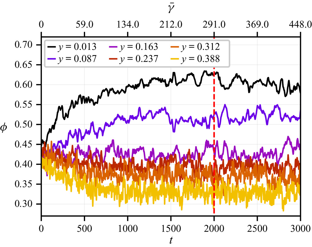
We focus first on the transient flow during which the volume fraction and velocity profiles develop. Figure 3 displays the time evolution of the volume fraction at various positions in the channel for the mean volume fraction  $\bar {\phi }=0.4$. The particle migration towards the channel centre is evidenced. Steady-state is reached approximately at time
 $t \approx 1000$, corresponding to the mean accumulated strain
 $\bar \gamma \approx 134$, except at the centre of the channel, where long-time migration is slower and a steady state seems to be reached at
 $t\approx 2000$ (
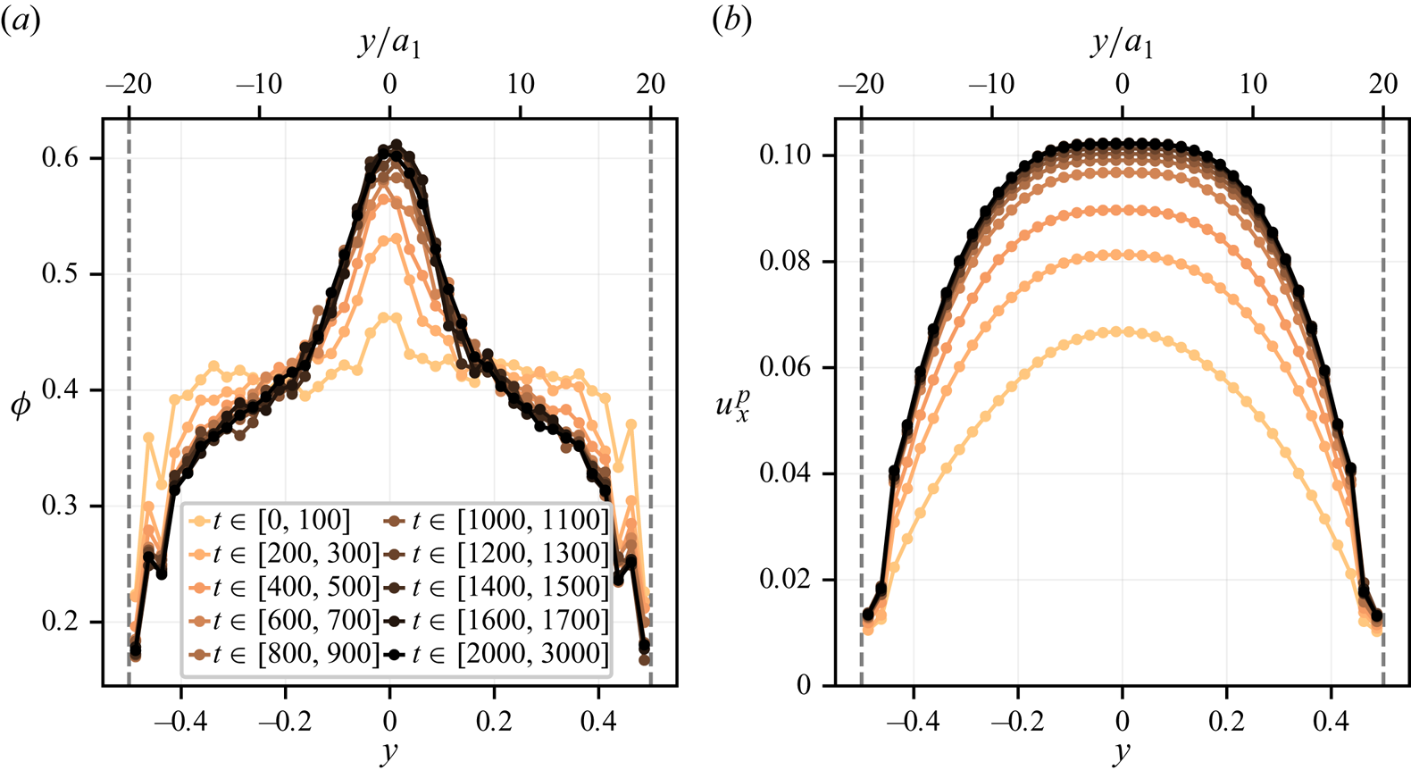
 $\bar \gamma \approx 291)$. The same data are used to plot the evolution of the volume fraction profile over time in figure 4(a). Each profile results from an averaging over the time interval
 $\Delta t=100$, which is enough to get rid of part of the statistical fluctuations. This interval is extended up to
 $\Delta t=1000$ for the steady state profile. The resulting profiles are reasonably smooth, except in the vicinity of the bounding walls, where layering occurs as expected, even though the suspension is bidisperse (Howard et al. Reference Howard, Maxey and Gallier2022, Reference Howard, Dong, Patel, D'Elia, Maxey and Stinis2023). We note that layering is not completely apparent due to our loose sampling. However, we clearly evidenced it in a previous article (Orsi et al. Reference Orsi, Lobry and Peters2023), where it was shown to extend over around
 $3a_1$ at
 $\bar {\phi }=0.45$. The corresponding particle velocity profiles are displayed in figure 4(b). A parabolic profile typical of a uniform viscosity field classically turns into a more blunted profile due to the viscosity variations that reflect the enhanced volume fraction at the channel centre. A significant wall slip is also evidenced, which originates in the mentioned layering. Such a wall slip has often been observed in experiments (Jana, Kapoor & Acrivos Reference Jana, Kapoor and Acrivos1995; Sarabian et al. Reference Sarabian, Firouznia, Metzger and Hormozi2019) or in simulations of monodisperse (Yeo & Maxey Reference Yeo and Maxey2011; Gallier et al. Reference Gallier, Lemaire, Peters and Lobry2014b, Reference Gallier, Lemaire, Lobry and Peters2016) and bidisperse (Howard et al. Reference Howard, Maxey and Gallier2022; Orsi et al. Reference Orsi, Lobry and Peters2023; Peerbooms et al. Reference Peerbooms, Nadorp, van der Heijden and Breugem2024) suspensions. We checked that the particle and suspension instantaneous velocity profiles are very close to each other, with a somewhat larger discrepancy in the layering area, as also shown at steady flow in § 5.2.
Time evolution of the volume fraction at different  $y$-positions in the channel for
 $\bar {\phi } = 0.4$. Averaging for steady flow starts from the vertical red line.
Volume fraction and velocity profiles during particle migration for  $\bar {\phi } = 0.4$. The vertical dashed lines indicate the volume boundaries.
In addition to the variation of the overall particle volume fraction, the spatial distribution of the small and large particles is computed. Figure 5 displays the time evolution of the volume fraction of small and large particles. A running average has been performed with a kernel of width  $\Delta T = 20$ to decrease the amplitude of the fast fluctuations. The small particle volume fraction approximately follows the evolution of the mean volume fraction, although at a slower rate. The variation of the large particle volume fraction is somewhat more complicated, with a faster variation at a small time, and long-time reorganization. On the whole, it seems that the latter is not complete at the end of the simulation.
Small ( $\phi _1$) and large (
 $\phi _2$) particles volume fraction as a function of time. Same simulation and legend as in figure 3. Upper scale is typical accumulated strain (2.17). High-frequency fluctuations have been averaged out using a simple running average (
 $\Delta T = 20$) to enhance readability. Same positions in the channel as in figure 3.
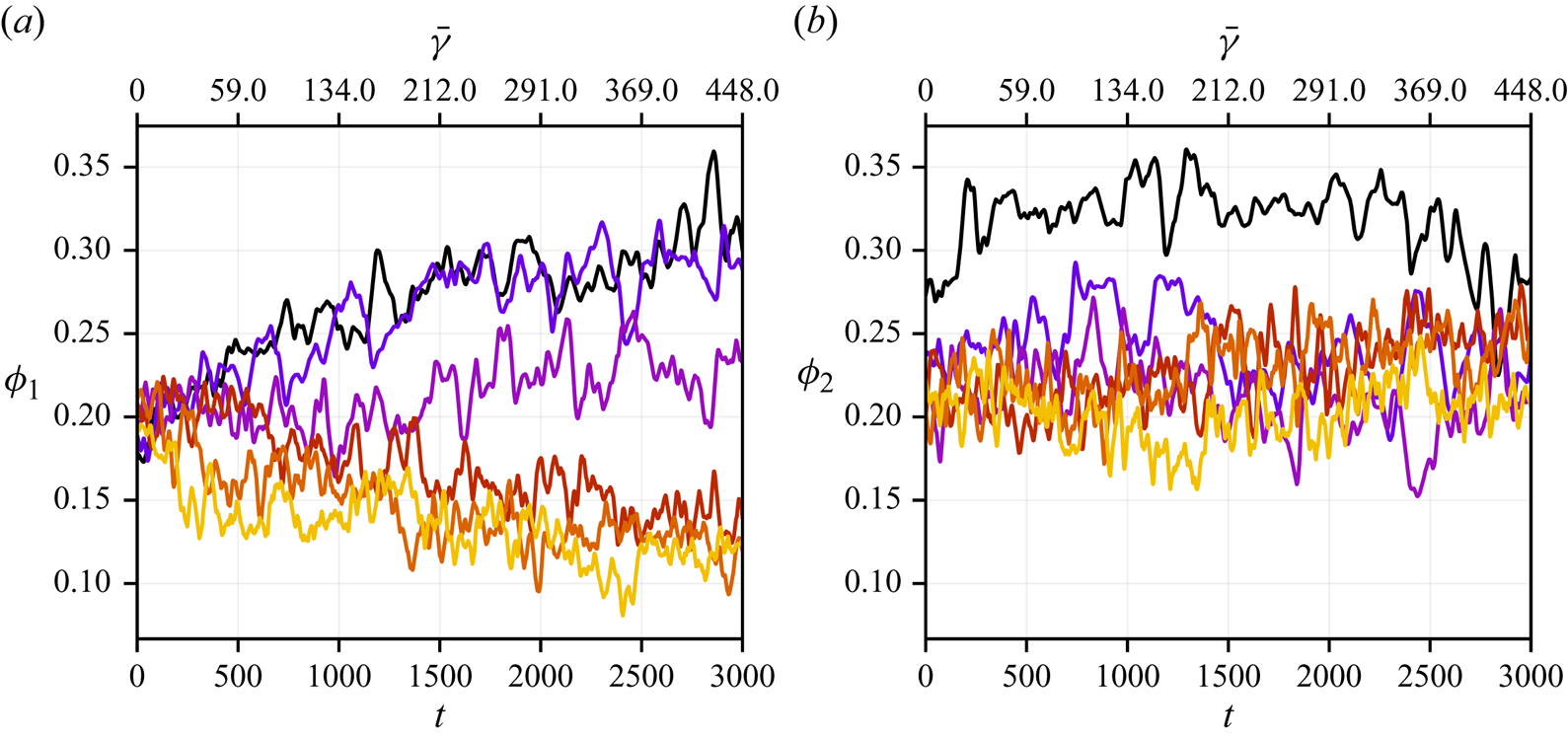
To get a clearer understanding of the evolution of both populations, the transient volume fraction profiles of the small and large particles are displayed in figure 6, both at the beginning (figure 6a,b) and at the end (figure 6c,d) of the simulation. At the beginning, a faster migration of the large particles takes place towards the channel centre, compared with the small particles, resulting in a peak of the large particle volume fraction at the centre, together with dips at the base of the peak. At larger time, reorganization of the particles occurs, with a deepening of the dips in the large particle volume fractions, together with the building of secondary peaks at the same position in the small particle volume fraction. It should be noted that during the time interval  $[900, 3000]$, the overall volume fraction profile only weakly evolves, mostly at the centre of the channel (figure 4).
Evolution with time of the small (a,c) and large (b,d) particle volume fraction profiles at the beginning (a,b) and at the end (c,d) of the simulations.  $\bar {\phi }=0.4$. Vertical dashed lines are boundary positions.

This is in qualitative agreement with the simulations of bidisperse suspensions,  $0.3$ in volume fraction, by Chun et al. (Reference Chun, Park, Jung and Won2019) who showed that particle segregation is much slower than the overall particle migration, except for a peak of the large particle volume fraction at the channel centre. We stress again that long-time particle reorganization seems to affect only weakly the total solid volume fraction and flow velocity profiles (figure 4). The time and accumulated strain for steady averaging are given in table 1 for each simulation.
5.2. Steady profiles
In the present section, we focus on the steady volume fraction and velocity profiles. Figure 7 displays the steady volume fraction profiles for all three values of the mean volume fraction  $\bar {\phi }$, together with the specific volume fraction profile for the large and small particles. The jamming volume fraction
 $\phi _J = 0.592$ deduced from simulations of homogeneous bidisperse suspensions in simple shear flow (§ 4) is also displayed. In the less concentrated case
 $\bar {\phi }=0.3$, the volume fraction at the channel centre does not reach
 $\phi _J$, in agreement with several experimental (Lyon & Leal Reference Lyon and Leal1998; Rashedi et al. Reference Rashedi, Sarabian, Firouznia, Roberts, Ovarlez and Hormozi2020) and numerical (Yeo & Maxey Reference Yeo and Maxey2011; Chun et al. Reference Chun, Park, Jung and Won2019; Howard et al. Reference Howard, Maxey and Gallier2022) studies. This is, however, in contrast to SBM predictions, according to which the volume fraction
 $\phi _J$ is reached at the channel centre whatever the mean volume fraction
 $\bar {\phi }$. Turning to the distribution of the large and small particles (
 $\phi _2$ and
 $\phi _1$, respectively), both migrate towards the centre, with approximately uniform composition
 $\phi _{2}/\phi \approx 0.5$ except at the bounding walls where only small particles are found. An explanation for the latter behaviour has been proposed by Howard et al. (Reference Howard, Maxey and Gallier2022) based on interactions between large and small particles close to a wall.
(a–c) Total volume fraction ( $\phi$), large (
 $\phi _2$) and small (
 $\phi _1$) particles volume fraction profiles at a steady flow. (d–f) Ratio of the large particles to overall solid volume fraction. Here (a,d)
 $\bar \phi = 0.3$; (b,e)
 $\bar \phi = 0.4$; (c,f)
 $\bar \phi = 0.5$.
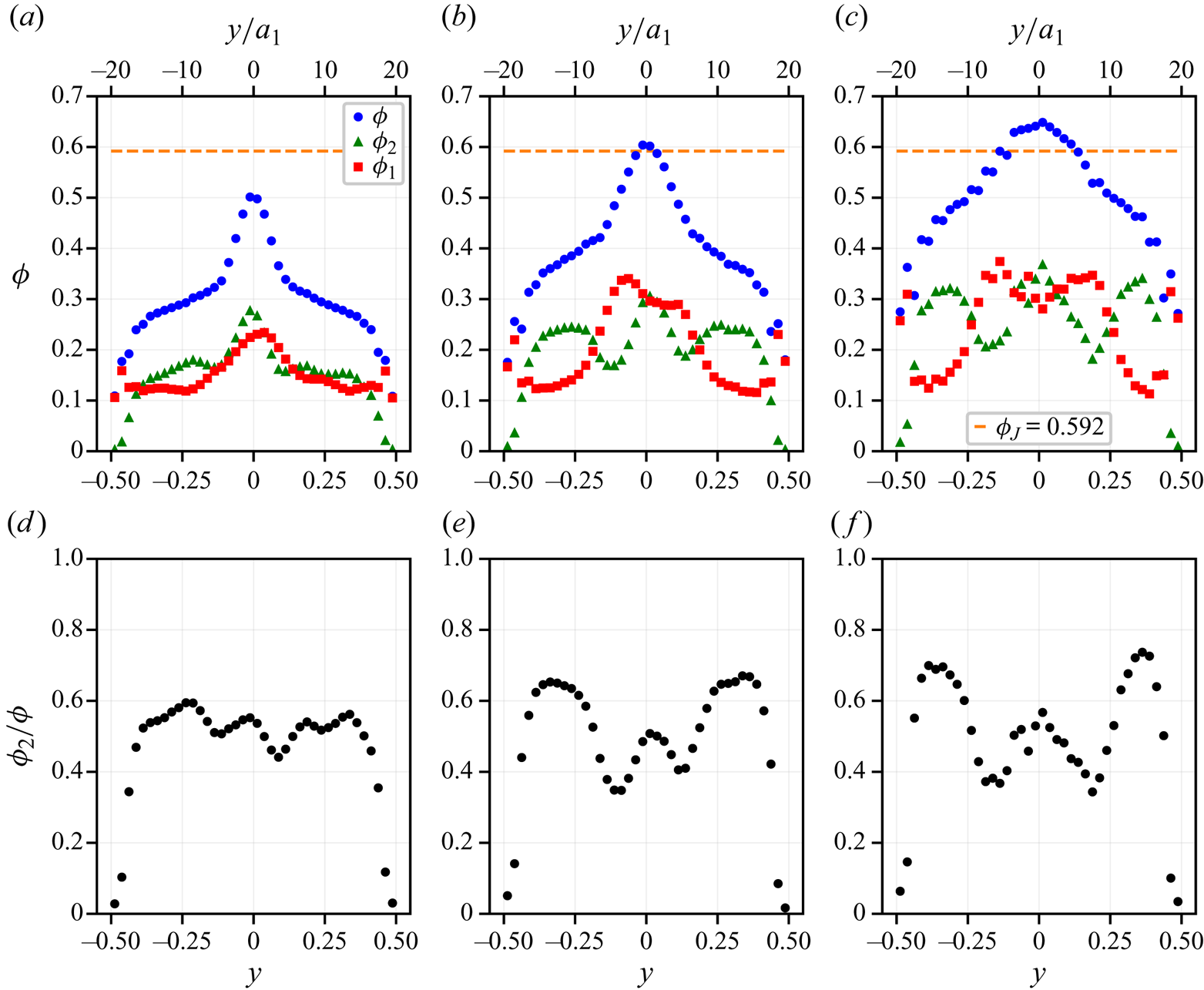
The simulations at larger mean volume fraction  $\bar {\phi }$ are somewhat different from the previous case. The overall volume fraction exceeds
 $\phi _J$ at the channel centre (the ‘plug’), over a width significantly larger than the particle size: at
 $\bar {\phi } = 0.5$, the volume fraction reaches
 $0.65$ and exceeds
 $\phi _J = 0.592$ over
 $10a_1$. Such a feature has been evidenced by Oh et al. (Reference Oh, Song, Garagash, Lecampion and Desroches2015) in their experiments on migration in non-Brownian suspensions of monodisperse particles in a pipe flow. They show that, for a large enough mean volume fraction, the volume fraction at the centreline of the tube levels off to a value close to the random close packing fraction
 $\phi _{rcp} \approx 0.64$. We note here that this value of the volume fraction is also known from simulation (Gallier et al. Reference Gallier, Lemaire, Peters and Lobry2014b; Mari et al. Reference Mari, Seto, Morris and Denn2014; Singh et al. Reference Singh, Mari, Denn and Morris2018; Chèvremont et al. Reference Chèvremont, Chareyre and Bodiguel2019) to be approximately the suspension jamming volume fraction when frictionless particles are considered. Regarding the local composition of the suspension, the large particle volume fraction presents a peak at the channel centre, as expected, but also two dips at a distance from the centre around
 $5a_1$. The small particles migrate towards the centre too, although with a peak at the positions of the previously mentioned dips. Leaving aside the layering area at the bounding wall, we note that the proportion of large particles
 $\phi _2/\phi$ varies over a quite wide range
 $[0.35, 0.74]$. Despite these variations, the overall volume fraction smoothly varies over the channel width.
The relative volume fraction profile at  $\bar {\phi }=0.4$ is in qualitative agreement with the data computed by Howard et al. (Reference Howard, Maxey and Gallier2022) for frictionless particles using the FCM, with slightly different ratio
 $a_2/a_1$ though, which parameter they show to have a clear influence on segregation. We note that the dips in the large particle volume fraction profile are less pronounced in their data. To check the influence of friction, we also performed a single simulation for frictionless particles, and we compare in figure 8 the volume fraction profile with data by Howard (Reference Howard2018), for the same ratio
 $a_2/a_1 = 1.4$ and mean volume fraction
 $\bar {\phi }=0.4$
Nearly steady total volume fraction profile ( $\phi$), large (
 $\phi _2$) and small (
 $\phi _1$) particles volume fraction profiles. Frictionless particles
 $\mu _s=0$. Symbols are short time average from FDM simulations. Lines are FCM simulations by Howard (Reference Howard2018). Vertical dashed lines are boundary positions.

We checked that the total volume fraction has approximately reached steady state at the observed total strain  $\bar {\gamma } = 325$, while the small and large particle concentration is still somewhat evolving. The agreement is very good. In particular, the marked dips in the large volume fraction profile observed close to the centre plane for frictional particles are significantly weaker for frictionless particles. Slight discrepancies may be observed, though, mainly in the total volume fraction profile. This may be explained by the larger system size that Howard (Reference Howard2018) and Howard et al. (Reference Howard, Maxey and Gallier2022) consider, namely
 $L_y = 56 a_1$. We note that in both simulations, the volume fraction remains lower than the jamming volume fraction for frictionless particles, i.e.
 $\phi _J^{\mu _s=0}\approx 0.64\hbox{--} 0.65$ (Mari et al. Reference Mari, Seto, Morris and Denn2014; Gallier, Peters & Lobry Reference Gallier, Peters and Lobry2018), even at the channel centre. This latter feature highlights the influence of friction, which increases the contact contribution to the stress (Gallier et al. Reference Gallier, Lemaire, Peters and Lobry2014b; Peerbooms et al. Reference Peerbooms, Nadorp, van der Heijden and Breugem2024), thereby enhancing particle migration, as implied by (3.15).
Back to frictional particles, figure 9 displays the particle and suspension axial velocity profiles, together with their relative difference. As already mentioned, the velocity profiles are blunted compared with the parabolic profile observed in a homogeneous Newtonian liquid. This is all the more the case as a larger value of  $\bar {\phi }$ is considered. It is also clear that the suspension and particle velocities are very close to each other, except in the layering area at the boundaries, where the difference grows while oscillating as the boundary is approached (the corresponding points are out of the scale in figure 9d–f).
(a–c) Particle ( $u_x^p$) and suspension (
 $u_x^s$) velocity profiles at a steady flow. (d–f) Profile of the relative difference between suspension and particle velocity. Same
 $\bar {\phi }$ as in figure 7.

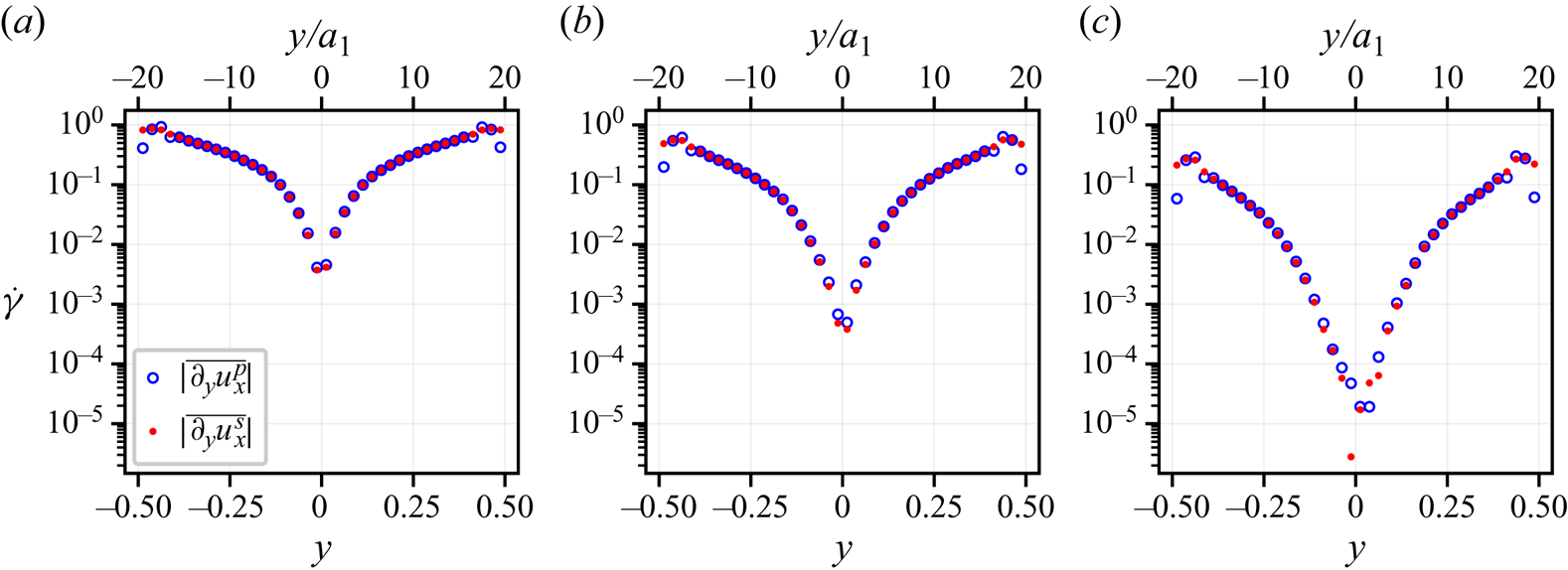
In particular, there is no significant difference between the shear rate as computed either from one or the other velocity profiles, except in the layering area. This is clearly illustrated in figure 10, where the shear rate profiles from the time-averaged velocity gradients over the steady flow duration, are displayed. The shear rate varies over two or three orders of magnitude, quite smoothly over the whole channel, except in the vicinity of the bounding walls, due to particle layering, and also at the channel centre, the latter only in the case of the largest mean volume fraction  $\bar {\phi }=0.5$. It should be stressed that the reliability of the shear-rate measurement is of importance since it is involved in the local determination of the constitutive laws. In particular, the time-averaged velocity gradient is expected to be exactly zero at the very centre of the channel and to be very small in the vicinity of the centreline. The relevance of such a small shear rate will now be addressed.
Shear rate profiles from the particle and suspension velocity profiles. Same values of  $\bar {\phi }$ as in figure 7.
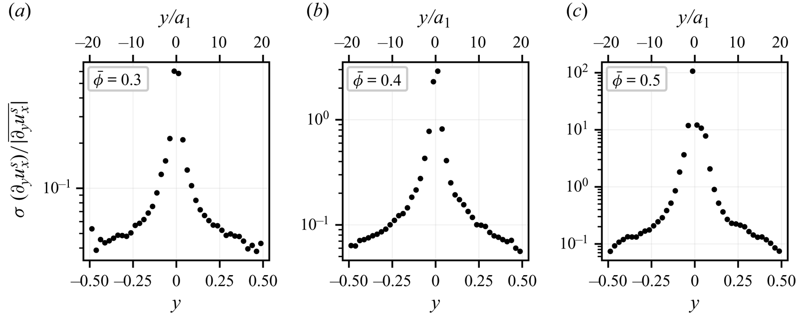
To gain some qualitative insight into this matter, the standard deviation of the velocity gradient is computed and compared with the average velocity gradient. In more detail, the velocity gradient profile is computed at each time step during the steady flow according to (4.1), yielding the time-averaged velocity gradient  $\overline {\partial _{y}u_x^{s}}$ and the standard deviation
 $\sigma (\partial _{y}u_x^{s})$ profiles. The ratio of the latter to the former is displayed in figure 11 for all three values of the mean volume fraction
 $\bar {\phi }$. In the region of the flow where this ratio is larger than typically unity, the fluctuations of the shear rate profile are sufficiently intense for the instantaneous shear rate to change sign frequently. In this case, the flow behaviour may differ significantly from a steady simple shear flow, yielding quite a different microstructure. While such large fluctuations are limited to a narrow region close to the centreline, typically
 $3-4a_1$ in width, at
 $\bar {\phi }=0.4$, they occur over a
 $10a_1$-wide region at
 $\bar {\phi }=0.5$. In both cases, the high fluctuations area also corresponds to the plug region where the volume fraction exceeds the jamming volume fraction as computed in a HSF, suggesting that the suspension is jammed. In the same line, the computed accumulated strain during steady state in that region is smaller than unity. At
 $\bar {\phi } = 0.3$, the relative standard deviation is always lower than unity, consistent with the largest observed volume fraction (
 $\approx$0.5) lower than
 $\phi _J$.
Relative standard deviation of the suspension velocity gradient: (a)  $\bar {\phi }=0.3$; (b)
 $\bar {\phi }=0.4$; (c)
 $\bar {\phi }=0.5$.
It is worth noting that the velocity gradient fluctuations computed from the particle velocity field (not displayed) do not differ from the suspension velocity gradient fluctuations.
6. Local stress constitutive laws
6.1. Momentum balance in steady flow
Before the local constitutive laws are addressed, the mechanical consistency of the numerical model will be checked. In the following section, the momentum balance for the suspension, i.e. (3.12) together with (4.6), is examined, in both the velocity and velocity gradient directions.
6.1.1. Tangential stress  $\varSigma _{xy}$

The  $x$-component of (3.12) is written as
 \begin{equation} {-}\dfrac{\mathrm{d}P_0}{\mathrm{d}\kern0.07em x} + \partial_y ( \eta \partial_y u_x^s +n\langle {\mathsf{S}}_{xy}^h \rangle _p + n\langle {\mathsf{S}}_{xy}^c \rangle _p )=0. \end{equation}
The first term is the imposed pressure gradient. The second and third terms constitute, respectively, the hydrodynamic contribution of the pure fluid and of the particles to the stress, while the last term is the contact force contribution. Equation (3.12) classically reflects that the tangential stress is driven by the pressure gradient. Its validity will be checked at steady flow in the following.
The total steady dimensionless shear stress profile is displayed in figure 12(a), together with the contact and hydrodynamic contributions, for the mean volume fraction  $\bar {\phi } = 0.4$. The theoretical shear stress
 $({\mathrm {d}P_0}/{\mathrm {d}\kern0.07em x})y$ (i.e.
 $4y$ in dimensionless form) computed from the imposed pressure gradient using (6.1) is also displayed. Except in the layering area, a very good agreement is found between the total shear stress profile and its theoretical expression, including symmetry and cancelling at the channel centre, reflecting the symmetry of the averaged stress boundary conditions. The momentum balance equation may also be examined in its direct, (6.1), and not integrated form in figure 12(b), where the force densities (i.e. the stress gradients) have been computed using numerical differentiation. The uniform tangential stress gradient again reflects the good local behaviour of the FDM numerical model.
(a) Steady tangential stress profile, together with contributions detailed in (6.1). (b) Corresponding force densities.  $\bar {\phi }= 0.4$.
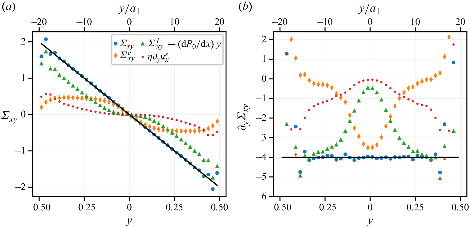
The quantitative relation between material functions and volume fraction will be addressed in detail in § 6.2. However, figure 12 allows qualitative inspection of the relative importance of the different contributions. The ratio of the contact contribution to the total shear stress increases with the volume fraction, and the contact contribution exceeds the hydrodynamic contribution when the volume fraction exceeds approximately  $0.42$, as expected from the usual constitutive laws in HSF (§ 6.2). We also note that the force density from the hydrodynamic shear stress exceeds the contact force density for
 $\vert y^* \vert \geq 0.11$, i.e. for
 $\phi \leq 0.5$.
Finally, the same curves as in figure 12 may be drawn for the other values of  $\bar {\phi }$. They are displayed in Appendix A (figures 28 and 29), with the same features as described above. It should be noted that the same general behaviour is observed during the transient migration, whether instantaneous quantities are considered, or short-time averaging is performed, with more intense fluctuations, though.
6.1.2. Normal stress $\varSigma _{yy}$

The  $y$-component of (3.12) is written as
 \begin{equation} \partial_{y}\varSigma_{yy} = \partial_{y}\varSigma_{yy}^{f} + \partial_{y}\varSigma_{yy}^{c} = 0. \end{equation}
The total  $yy$ component of the total stress is expected to be uniform, meaning that the variation of the fluid stress should compensate for the variation of the contact contribution. This behaviour is observed in figure 13(a), except in the layering area close to the walls, both at the beginning of the simulation and during steady flow, when migration is complete. Uniformity of the total stress is especially striking when the solid volume fraction is homogeneous as the simulation starts, since both the fluid and solid contributions are strongly non-uniform, in agreement with the SBM according to which the particles are pushed towards the channel centre due to the divergence of the contact stress, (3.15).
Total stress profile (a) together with fluid (b) and contact (c) contributions, at the beginning of the simulation and during steady flow:  $\bar {\phi } = 0.4$.

When particle migration is complete, both the fluid and contact contributions are uniform, in agreement with the SBM, except at the channel centre, where a weak stress gradient persists. The latter is not predicted by the SBM. However, the fluid and contact contributions still counterbalance each other.
Again, the corresponding curves for  $\bar {\phi } = 0.3$ and
 $0.5$ are displayed in Appendix A.2 (figures 30 and 31). The total stress is uniform as well for both volume fraction values. However, in the case of the lower mean volume fraction,
 $\bar {\phi } = 0.3$, the contact and fluid stresses are slightly non-uniform after the migration is finished. This will be discussed in § 7.
6.2. Local constitutive laws
The goal of the present section is to determine to what extent the main constitutive laws evidenced in HSF simulations still locally hold in the pressure-driven flow. To keep the noise level low, all needed quantities are averaged over the steady flow duration. The main results displayed here will be discussed in § 6.3. Also displayed are the correlation laws for the normal stress differences and for the reduced contact stresses by Badia et al. (Reference Badia, D'Angelo, Peters and Lobry2022) which were fitted onto particle resolved simulations of bidisperse suspensions for the same friction coefficient  $\mu _s=0.5$. We note that such correlation laws, with slightly different numerical coefficients, were recently found to satisfactorily describe simulated quantities for various values of the friction coefficients (Peerbooms et al. Reference Peerbooms, Nadorp, van der Heijden and Breugem2024). Before turning to the material functions, the measurement resolution is briefly discussed.
6.2.1. Spatial sampling and resolution
At this point, the choice of the spatial sampling period together with the measurement resolution deserve a few words. From a purely numerical point of view, the smallest length scale that we can probe is the solver mesh size, which is  $0.2 a_1$. However, as explained in § 4.1, the averaging process for the quantities that are computed from particle-related quantities, e.g. the contact force density from the contact forces exerted on each particle, involve two different steps. Each particle quantity, denoted by
 $Y_p$ in (4.5), is computed as a volume integral over the particle volume, and then evenly spread over the particle volume before the local averaging is performed, (4.5). As a consequence, the averaging procedure itself introduces a correlation length equal to the particle radius, and it seems not relevant to probe the quantities at a shorter length scale. There are some exceptions to this general rule, since some quantities do not suffer from this limitation. For instance, if the particle layering near the wall is to be studied, the volume fraction profile at smaller scale is indeed relevant (Yeo & Maxey Reference Yeo and Maxey2010; Gallier et al. Reference Gallier, Lemaire, Lobry and Peters2016; Howard et al. Reference Howard, Maxey and Gallier2022). However, such a study is not the primary goal of the present paper, and hence we chose
 $a_1$ as the smallest relevant spatial sampling period
 $\Delta y$.
The resolution of the measurement is then a matter of statistical fluctuations, whose intensity are expected to decrease with the spatial averaging size (i.e.  $L_x \times L_z$) and the time averaging duration. The precise determination of the statistical error in transient flow did not seem feasible to us, at least at a reasonable computation cost, since it would imply repeating each run (several weeks using 128 cores) approximately 10 times. However, in steady flow, standard techniques are available that allow us to determine quite precisely the standard error (Allen & Tildesley Reference Allen and Tildesley2017). For the sake of figure clarity, the error bars are not included in the main text figures, but are displayed in the corresponding figures in Appendix B. Finally, we checked that choosing
 $\Delta y = 2a_1$ would not significantly change the measured material functions.
6.2.2. Shear viscosity
The steady relative viscosity is computed from the time-averaged shear stress and the time-averaged suspension velocity gradient  $\eta _S = \overline {\varSigma _{xy}}/(\eta \overline {\partial _y u^s_x})$ at each position in the channel. It is displayed as a function of the solid volume fraction
 $\phi$ for
 $\bar {\phi }=0.4$ in figure 14(a), together with the corresponding data from HSF simulations (Orsi et al. Reference Orsi, Lobry and Peters2023). The agreement is very good in an intermediate region, not too close to the wall or the centreline. Discrepancies are evidenced in the vicinity of the bounding walls (low volume fraction), where layering occurs, and in a central area (high volume fraction), approximately
 $9a_1$ in width. The data for which reasonable agreement is empirically found are highlighted in figure 14(a). The corresponding region is denoted by ‘the intermediate area’ in the following. The same procedure is repeated for the other simulations. The local viscosity data over the whole channel are displayed for all values of
 $\bar {\phi }$ in Appendix B.1 (figure 32), and the data from the intermediate region are gathered in figure 14(b), showing again very good agreement over a wide volume fraction range
 $0.27 \leq \phi \leq 0.55$. Also displayed is the Maron–Pierce correlation law, which has been fitted onto the data from HSF simulations,
 \begin{equation} \eta_S = \dfrac{\alpha}{(1 - \phi / \phi_J )^2}, \end{equation}
yielding the jamming volume fraction  $\phi _J = 0.592$.
Viscosity as a function of local volume fraction. Here (a)  $\bar {\phi }=0.4$. (b) All simulations. Here (
 $\bullet$, blue)
 $\bar {\phi }=0.3$, (
 $\blacklozenge$, orange)
 $\bar {\phi }=0.4$, (
 $\blacktriangledown$, green)
 $\bar {\phi }=0.5$. Black symbols are HSF simulations; plain line is (6.3) with
 $\phi _J = 0.592$ and
 $\alpha = 0.8$.
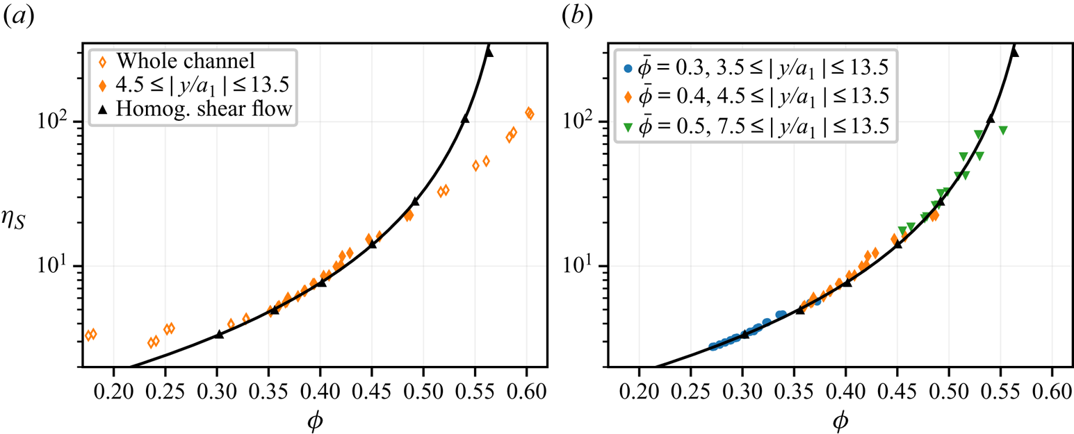
We note (Appendix B.1, figure 32) that in the central region, for all simulations, the computed reduced viscosity is below its counterpart in HSF. In addition, no divergence is observed at the channel centre, which is allowed by the simultaneous vanishing of the shear stress and the shear rate. Finally,  $\eta _S$ seems to be defined in the ‘jammed’ phase where
 $\phi >\phi _J$. However, as mentioned previously, the computed shear rate suffers from very high fluctuations in that region, making the reliability of its averaged value questionable.
For the sake of completeness, the various relative contributions to the viscosity, or equivalently the relative contributions to the shear stress, are displayed in figure 15 for the intermediate region. The relative hydrodynamic contribution to the viscosity is split into the pure fluid contribution equal to unity, the particle solver and subgrid contributions, denoted, respectively, by  $\eta _{FDM}$ and
 $\eta _{SG}$:
 \begin{equation} \eta_{\boldsymbol{\mathsf{S}}} = 1 + \dfrac{n \langle {\mathsf{S}}_{xy}^{FDM}\rangle _p + n \langle S_{xy}^{SG}\rangle _p + n \langle S_{xy}^{c}\rangle _p } { \eta\ \langle \partial _y u^s_x \rangle} = 1+\eta_{FDM}+\eta_{SG}+\eta_{c}. \end{equation}
The data are in excellent agreement with those from HSF simulations. The relative contribution of the contact forces to the viscosity, i.e.  $\hat \varSigma _{12}^c$ (4.10), is displayed for the three values of
 $\bar {\phi }$ in figure 35 (Appendix B.3). It turns out that in the central area, where the usual expression for the viscosity does not hold, the relative contact contribution is smaller than expected. This feature, together with the low value of the computed relative viscosity in the same region, suggests that the force microstructure is significantly different compared with what prevails in HSF. It should be noted that this behaviour is not limited to the region where
 $\phi > \phi _J$.
Relative contributions to the shear viscosity in the intermediate region: (a) contact and hydrodynamic contributions; (b) FDM contribution; (c) subgrid contribution; (d) pure fluid contribution. Same colour code as in figure 14(b).
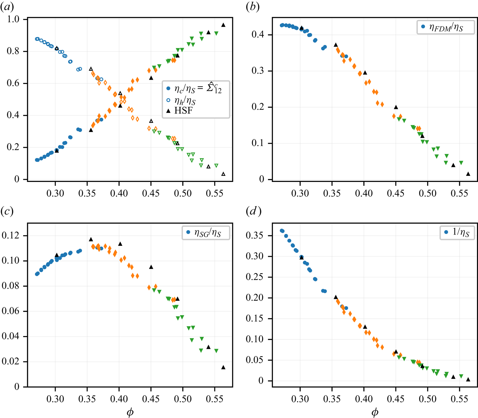
6.2.3. Normal stress differences
The reduced first ( $\hat N_1$) and second (
 $\hat N_2$) normal stress differences in the intermediate region are displayed in figure 16. The data from the pressure-driven flow simulations are in reasonable agreement with the HSF data, although over a narrower position range compared with the shear viscosity. We note that, for
 $\bar {\phi } = 0.3$ and
 $0.4$ the discrepancy starts at the same position as the volume fraction gradient significantly increases, which corresponds, for
 $\bar {\phi } = 0.4$, to the position where the small particle volume fraction exceeds its counterpart for the large particles. However, a significant discrepancy is observed over the whole channel at
 $\phi =0.5$ for the first normal stress difference. Regarding the central region (Appendix B.2, figure 33), we also note that the values of the first normal stress difference largely differ from the HSF correlation, including its sign, which again suggests a different microstructure in this area.
Reduced normal stress differences in the intermediate region. Same colour code as in figure 14(b). Plain line is correlation law by Badia et al. (Reference Badia, D'Angelo, Peters and Lobry2022).

6.2.4. Contact normal stresses
The present section is devoted to the constitutive laws that define contact normal stresses. Since the latter, especially  $\hat \varSigma _{22}^c$ in the present case, are involved in the particle transverse velocity, (3.15), and consequently in the solid volume transport equation, (3.18), it is worth checking that the laws deduced from HSF simulations still hold in the present pressure-driven flow. All three contact stresses are displayed in figure 17 for all simulations, in the volume fraction range that corresponds to the intermediate region of each run. Again, a good agreement with HSF simulations is observed, although the reduced normal stresses as computed here are slightly larger than the HSF data.
Reduced contact normal stresses in the intermediate region. Same colour code as in figure 14(b). Plain line is correlation law by Badia et al. (Reference Badia, D'Angelo, Peters and Lobry2022).

In the central region, the HSF constitutive laws for the contact normal stresses hold better compared with the shear viscosity (Appendix B.4, figures 36–38). Even though at the centre of the channel, where the tangential stress vanishes, the reduced contact stresses diverge, consistent with the non-vanishing contact normal stresses at this position, it is, however, striking that at  $\bar {\phi } = 0.3$, the discrepancy is only noticeable for
 $\vert y \vert \leq a_1$ or only for
 $\phi \geq \phi _J$ in the two most concentrated cases.
6.2.5. The $\mu (J)$ rheology

Finally, the  $\mu$-rheology (Boyer et al. Reference Boyer, Guazzelli and Pouliquen2011) is computed. The macroscopic friction coefficient
 $\mu = \varSigma _{xy}/\varSigma _{yy}^c$ and volume fraction are displayed as a function of the viscous number
 $J=\eta \dot {\gamma }/\varSigma _{yy}^c$ in figure 18(a,b), respectively, together with the HSF results. A good agreement is found in the intermediate region for both quantities. Several correlation laws are available in the literature. In the present paper, we compare our simulation data with the experimental laws by Boyer et al. (Reference Boyer, Guazzelli and Pouliquen2011) and to the correlation laws fitted on our own earlier simulations for a microscopic friction coefficient
 $\mu _s=0.5$ (Badia et al. Reference Badia, D'Angelo, Peters and Lobry2022). We note that recent numerical studies extensively investigated the influence of the friction coefficient
 $\mu _s$ on these correlation laws (Chèvremont et al. Reference Chèvremont, Chareyre and Bodiguel2019; Peerbooms et al. Reference Peerbooms, Nadorp, van der Heijden and Breugem2024). The displayed correlation laws deserve a few words. The correlation laws by Badia et al. (Reference Badia, D'Angelo, Peters and Lobry2022) have been fitted onto data concerning moderately concentrated to concentrated suspensions (
 $\phi \le 0.56$) at
 $\mu _s=0.5$, which explains why they are close to the HSF data, in particular the macroscopic friction coefficient
 $\mu$, for the whole range of viscous number
 $J\in [2.10^{-3}, 2]$. However, the limit of
 $\mu$ for vanishing
 $J$ may not be considered, since it was not confirmed by simulation data. On the other hand, the experimental correlation laws by Boyer et al. (Reference Boyer, Guazzelli and Pouliquen2011) were tuned for small values of
 $J$ (
 $\lesssim 0.2$) and thus may not perfectly fit the high
 $J$ range (d'Ambrosio, Blanc & Lemaire Reference d'Ambrosio, Blanc and Lemaire2023).
Macroscopic friction coefficient  $\mu$ (a) and volume fraction (b) as a function of viscous number
 $J$ in the intermediate region. Same colour code as in figure 14(b). Plain line is correlation by Badia et al. (Reference Badia, D'Angelo, Peters and Lobry2022), dashed line is correlation by Boyer et al. (Reference Boyer, Guazzelli and Pouliquen2011)

In the central region, the macroscopic friction coefficient  $\mu$ is lower than its counterpart in HSF, as displayed in Appendix B.5 (figures 39 and 40). This may be qualitatively checked in figures 12 and 13, where the shear stress
 $\varSigma _{xy}$ and the shear rate
 $\dot \gamma$ vanish at the channel centre, while the contact stress
 $\varSigma _{yy}^c$ does not, meaning that
 $\mu$ goes to zero at vanishing
 $J$, while it is expected to level off to a value close to
 $0.3$ in HSF (Boyer et al. Reference Boyer, Guazzelli and Pouliquen2011; Gallier et al. Reference Gallier, Lemaire, Peters and Lobry2014b). In the same region, the local volume fraction is larger than predicted by the HSF law.
This is to be compared with the numerical study of highly concentrated frictionless non-Brownian suspensions by Bhowmik & Ness (Reference Bhowmik and Ness2024), who use Kolmogorov flow to induce non-homogeneous shear rate and particle migration. They also observe discrepancies between HSF constitutive laws at positions where the shear rate vanishes or is small. More specifically, the macroscopic friction coefficient  $\mu$ decreases towards zero as the viscous number decreases, as in the present work.
6.3. Discussion
The previous sections allowed evidence of an intermediate region where the HSF constitutive laws reasonably hold, in agreement with the simulations of frictionless particle suspensions by Yeo & Maxey (Reference Yeo and Maxey2011), meaning that all data from this intermediate region in all simulations collapse onto the HSF curve. This may be surprising, given the significant particle segregation occurring. It is indeed well known that the viscosity of bidisperse suspensions depends on the particle size ratio  $a_2/a_1$ and volume fraction ratio
 $\phi _2/\phi$, mainly due to the effect of these parameters on the jamming volume fraction (Chang & Powell Reference Chang and Powell1994). Pednekar, Chun & Morris (Reference Pednekar, Chun and Morris2018) performed extensive simulations of concentrated non-Brownian bidisperse suspensions in the range
 $2 \leq a_2/a_1 \leq 4$ and
 $0 \leq \phi _2 /\phi \leq 1$, and with interparticle friction coefficient
 $\mu _s=0.2$. They confirmed that the jamming volume fraction reaches a maximum around
 $\phi _2 /\phi =0.6$, corresponding to a minimum of the viscosity for a given value of
 $\phi$. To extrapolate their results to the suspensions of interest here (
 $\mu _s=0.5$,
 $a_2/a_1=1.4$), and following Howard et al. (Reference Howard, Maxey and Gallier2022), we estimate the jamming volume fraction using
 \begin{equation} \phi_J = \phi_J^{mono} \left[ 1 + 1.5 \left(\dfrac{1 - a_1/a_2}{1 + a_1/a_2}\right)^{3/2}\left( \dfrac{\phi_2}{\phi}\right)^{3/2}\dfrac{\phi_1}{\phi} \right], \end{equation}
which we found in qualitative agreement with the data by Pednekar et al. (Reference Pednekar, Chun and Morris2018) and also with the proposed empirical expression of the packing fraction as a function of the moments of the size distribution by Desmond & Weeks (Reference Desmond and Weeks2014). In the present case, the monodisperse jamming volume fraction  $\phi _J^{mono}=0.582$ is estimated from
 $\phi _J(\phi _2/\phi = 0.5) = 0.592$ (§ 6.2.2). For the observed large particle volume fraction range
 $0.35\leq \phi _2/\phi \leq 0.70$, the absolute variation of
 $\phi _J$ is expected to keep under
 $0.003$. The observed segregation is thus expected to have a negligible effect on the data displayed in figure 14(b). More generally, it was previously noted that, despite segregation, the total volume fraction varies smoothly over the channel, except in the vicinity of the bounding walls. In addition, even though the distribution of small and large particles is not symmetric with respect to the channel centre plane, the overall volume fraction and velocity profiles are. In the same line, the simulations by Howard et al. (Reference Howard, Maxey and Gallier2022) of frictionless bidisperse suspensions with
 $a_1/a_2 = 0.7$ showed that the steady solid volume fraction profile only weakly depends on the initial value of
 $\phi _2/\phi$, suggesting that overall particle migration develops quite independently of segregation, at least for a size ratio
 $a_1/a_2$ close to unity. A possible explanation of this behaviour is the fact that, as evidenced by Howard et al. (Reference Howard, Maxey and Gallier2022), the stresses developing in a bidisperse suspension weakly depend on the composition
 $\phi _2/\phi$.
We also note that in the intermediate region identified as the positions where HSF constitutive laws hold for the shear viscosity, the reduced first normal stress difference,  $\hat N_1$, and to a lesser extent
 $\hat N_2$, display significant discrepancies. We do not exactly understand the origin of this behaviour. It seems to be correlated to a stiffening of the volume fraction profile, which is more or less concomitant to the dips in the large particle volume fractions. However, it is well known that the first normal stress difference is a subtle quantity, with quite low values, and which is expected to depend on the exact flow conditions and suspension microstructure to a greater extent compared with the shear viscosity or contact normal stresses.
Outside this intermediate area, the simulations allowed evidence of two regions where HSF constitutive laws do not hold, i.e. the layering area close to the boundaries, and the central region where the shear rate and shear stress go to zero. The former belongs to the general issue of wall effects. In agreement with earlier studies from the literature, we observe both particle layering and large particle depletion at the walls (Yeo & Maxey Reference Yeo and Maxey2011; Chun et al. Reference Chun, Park, Jung and Won2019; Howard et al. Reference Howard, Maxey and Gallier2022), and alterations of the bulk HSF stress constitutive laws are indeed expected (Gallier et al. Reference Gallier, Lemaire, Lobry and Peters2016; Peerbooms et al. Reference Peerbooms, Nadorp, van der Heijden and Breugem2024). We will not address this specific issue. We also note that an explanation of the depletion of the large particle has been recently proposed by Howard et al. (Reference Howard, Maxey and Gallier2022).
In the central region, two features deserve to be highlighted. It is first striking that the volume fraction may exceed the jamming volume fraction  $\phi _J$ for
 $\bar {\phi }\geq 0.4$. In the corresponding part of the flow, the mean computed shear rate is not zero but the large fluctuations, together with the low accumulated strain during steady flow make this estimation questionable, suggesting that the suspension is nearly jammed, even though fluctuations allow particle reorganization leading to
 $\phi \geq \phi _J$.
In addition, the constitutive laws as measured in HSF do not hold, meaning in particular that for each material function as computed from the various simulations in the central region, the data does not collapse onto a single curve when displayed as a function of the volume fraction. This behaviour is generally not limited to the plug region where  $\phi \geq \phi _J$. Leaving aside the very centre of the channel, the shear viscosity is smaller, the relative contribution of the contact forces to the shear stress
 $\hat \varSigma ^c_{12}$ is smaller, while the relative contact normal stresses
 $\hat \varSigma _{ii}^c$ follow the usual HSF law. In the frame of the
 $\mu (J)$ representation, this region corresponds to a lower
 $\mu$ than expected from HSF. At the very centre of the channel, the discrepancy is even more pronounced, since the contact normal stresses remain finite while the shear stress vanishes, leading to the divergence of the reduced normal stresses
 $\hat \varSigma _{ii}^c(\phi )$ (Appendix B.4, figures 36–38), or equivalently faster vanishing of
 $\mu (J)$ at low
 $J$ (Appendix B.5, figures 39 and 40).
As mentioned in the introduction, the pressure-driven flow of suspensions at the vicinity of the centre of the channel or the pipe has raised questions for a long time, in an attempt to understand particle migration (Nott & Brady Reference Nott and Brady1994; Mills & Snabre Reference Mills and Snabre1995; Morris & Boulay Reference Morris and Boulay1999; Miller & Morris Reference Miller and Morris2006), and more generally stress constitutive laws (Gillissen & Ness Reference Gillissen and Ness2020; Bhowmik & Ness Reference Bhowmik and Ness2024). The fact that the shear rate and shear stress vanish at the centre results in a strong relative variation of these quantities at the scale of a particle radius. It is most easily understood in the case of the shear stress, whose averaged value depends linearly on the  $y$-position from the channel centre plane, so that its variation at the scale of a particle may be estimated as
 $\Delta \varSigma _{xy}/\varSigma _{xy}\sim a_1/y$. As a consequence, non-local effects are expected to play a significant role at this position of the flow, all the more when normal stresses (or contact pressure) are involved, since for instance in steady shear, they are compressive whatever the sign of the shear stress, and as a consequence may not vanish as the shear stress fluctuates around zero. In the past, such effects have been included in the constitutive law for the normal stresses in different ways, either considering granular temperature contribution to the stress (Nott & Brady Reference Nott and Brady1994), space-averaged stresses (Mills & Snabre Reference Mills and Snabre1995; Morris & Boulay Reference Morris and Boulay1999) or adding a small non-local positive shear rate for the computation of the normal stresses (Miller & Morris Reference Miller and Morris2006). More recently, fluctuations have been explicitly included in a model, where the whole stress tensor depends on both the local shear-induced microstructure and the local shear-rate tensor (Gillissen & Ness Reference Gillissen and Ness2020). The idea is that the fluctuations of the shear rate tensor contribute to the mean compressive shear rate, and as a result to the compressive normal stresses, even though the mean shear rate and shear stress vanish. The model shows qualitative agreement with particle scale simulations, predicting in particular
 $\lim _{J \rightarrow 0} \mu (J)=0$. In the same line, it has been proposed that a new dimensionless number accounting for particle velocity fluctuations be included in the steady flow stress law, in addition to the usual viscous number
 $J$ (Bhowmik & Ness Reference Bhowmik and Ness2024).
In the present paper, we do not want to go too deep into the fluctuations at the particle scale, but we leave it instead for a future study. In § 5.2, we considered the fluctuations of the shear rate profile, i.e. a quantity that has already been averaged over the  $x$ and
 $z$ directions. As previously mentioned, the positions for which
 $\phi \geq \phi _J$ correspond to large values of the velocity gradient fluctuations
 $\sigma (\partial _{y}u_x^{s})\geq \vert \overline {\partial _{y}u_x^{s}}\vert$ and low values of the accumulated strain during the shear flow, suggesting a quasijammed suspension. As shown in figures 11 and 36–38 (Appendix B.4), those positions also correspond to most of the points where the values of the reduced contact normal stresses
 $\hat \varSigma _{ii}^c$ are significantly larger than predicted in HSF, the latter being approximately defined by
 $\sigma (\partial _{y}u_x^{s})\geq 0.5 \vert \overline {\partial _{y}u_x^{s}}\vert$. Except for this ‘jammed’ region, the central area, where the HSF laws do not hold, is only a few particle radii wide, corresponding to large volume fraction variation. These features naturally point to non-local effects, where the stresses also depend on the volume fraction and shear rate at a distance from the considered position. We finally note that experiments (Guasto, Ross & Gollub Reference Guasto, Ross and Gollub2010) and simulations (Yeo & Maxey Reference Yeo and Maxey2011) have evidenced long-range correlated motion at the centre of the channel that strengthens the hypothesis of non-local behaviour.
7. Investigation of the SBM hypothesis
As recalled in § 3, the main assumption of the SBM is (3.13), which connects the hydrodynamic force density applied to the particles to their transverse velocity, or equivalently to the solid flux density, as written in the present flow geometry:
 \begin{equation} u_y^p - u_y^s = \dfrac{2a^2}{9 \eta} \dfrac{f(\phi)}{\phi}\partial_y \varSigma_{yy}^c. \end{equation}
Before this issue is tackled in § 7.3, the transverse velocity will be examined in the following section, and the relation between the various force densities of interest and the gradient of the relevant stresses will be evidenced in § 7.2. Unless otherwise stated, every quantity is time-averaged over  $\Delta t = 200$ corresponding to a typical averaged strain
 $\bar {\gamma }\sim 10\hbox{--} 50$, depending on the mean volume fraction
 $\bar {\phi }$.
7.1. Transverse velocity
The transverse particle velocity relative to the suspension, which is related to the particle volume flux density (4.3), is displayed in figure 19 at various times during the transient flow. It is directed towards the channel centre, with a higher intensity at the start of the flow, and as expected vanishes as the steady state is reached. Its magnitude is very low compared with the amplitude of the main flow velocity, at most  $0.1\,\%$. We checked that
 $u_y^s$, which is computed from the solver velocity, is nearly zero, e.g. at
 $\bar {\phi }=0.4$ around
 $2 \times 10^{-6}$, in agreement with the incompressibility of the flow that is stated in (3.4). We checked that the fluctuations of the transverse particle velocity averaged over the whole steady flow duration are significantly larger than this residual transverse suspension velocity.
Transverse particle relative velocity,  $\bar {\phi } =0.4$. Averaging time is
 $\Delta t = 200$.

7.2. Various force densities exerted on the particle phase
As recalled by Lhuillier (Reference Lhuillier2009), the momentum balance equation for the particle phase, (3.5), is equivalent to (3.8). The latter does not need checking, since it directly originates from the single particle momentum balance equation (2.4), which was double-checked during the validation of the simulation code. However, other relations, such as the relation between the contact force density and the divergence of the contact stress (3.7), deserve a closer look. In the following, the various force densities at play are displayed, and their relations to the relevant stress gradients are evidenced.
7.2.1. Contact force density
According to the SBM, particle migration is driven by the contact force density  $n \langle f_y^c \rangle _p$, which is counterbalanced by the hydrodynamic drag force, yielding the particle volume flux. The former should also be equal to the divergence of the contact stress,
 $\partial _y \varSigma _{yy}^c$ (3.7), according to a theoretical analysis for pairwise interaction forces between particles (Irving & Kirkwood Reference Irving and Kirkwood1950; Jackson Reference Jackson1997). Equation (3.7) is expected to hold provided that the length scale defining the variation of averaged quantities is sufficiently large compared with the particle radius. It will be now examined. The contact force density along the
 $y$ direction is displayed in figure 20 for all simulations at the beginning of the flow and during steady flow after the migration is complete, together with the divergence of the contact stress along the same direction. The latter is computed from the contact stress by numerical differentiation (central difference). A very good agreement is observed, except in the layering region though, which discrepancy may be easily understood, given that all averaged quantities strongly vary at the particle scale in that region (Howard et al. Reference Howard, Maxey and Gallier2022; Orsi et al. Reference Orsi, Lobry and Peters2023). We stress that the force density and contact stress are independently computed, the former from the total contact force exerted on each particle, and the latter from the total contact stresslet. In addition, only two instants are considered here for the sake of figure clarity, but we checked that (3.7) holds at any time.
Transverse contact force density and its counterpart from the contact stress: solid symbol,  $t\in [0,\, 200]$; open symbol, steady flow (averaging time in table 1); (a)
 $\bar {\phi }=0.3$; (b)
 $\bar {\phi }=0.4$; (c)
 $\bar {\phi }=0.5$.
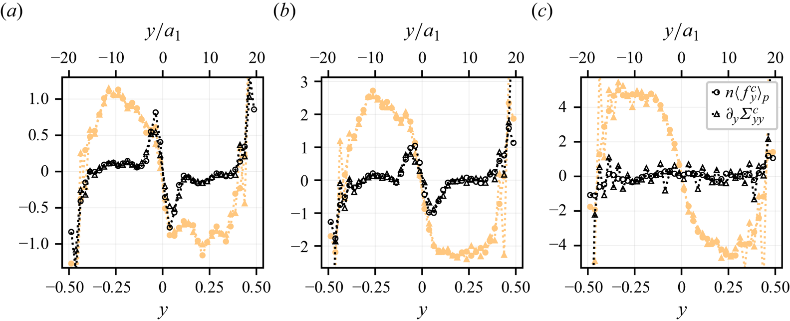
As expected, the contact force density pushes the particles towards the channel centre at the beginning of the simulation, and approximately vanishes at the end of transient migration, at least in the intermediate region. In the central region, two force peaks remain after migration is complete at  $\bar {\phi }=0.3$ and
 $\bar {\phi }=0.4$, which correspond to the dip observed in the contact stress profile, as already mentioned in § 6.1.2. At
 $\bar {\phi }=0.3$, a small force density also remains in the intermediate region after migration completion, which does not induce any net particle volume flux. This will be discussed in the following.
7.2.2. Hydrodynamic force density
The hydrodynamic force density  $n \langle f_y^h \rangle _p$ is exactly the opposite of the contact force density, due to the absence of inertia in the motion of each particle, (2.4). In addition, (3.9), which connects the hydrodynamic force density exerted on the particles to the divergence of the fluid stress in the
 $y$ direction, may be understood as the consequence of (3.7), (3.8), (3.11) and (3.12), which have already been shown to apply. However, inspection of the various contributions of the normal stress
 $\varSigma _{yy}^f$ is instructive. Equations (2.10), (2.9) and (4.6) yield
 \begin{align} \varSigma_{yy}^f &={-}(1-\phi)\langle p \rangle ^f + n\left\langle S_{yy}^{FDM} + \dfrac{s^{FDM}}{3}\right\rangle _p + n\left\langle S_{yy}^{SG} + \dfrac{s^{SG}}{3}\right\rangle _p \nonumber\\ &={-}(1-\phi)\langle p \rangle ^f +\varSigma_{yy}^{FDM} +\varSigma_{yy}^{SG}, \end{align}
where  $\varSigma _{yy}^{FDM}$ is computed from the force density
 $\boldsymbol{\lambda}$ and pressure perturbation
 $p$ inside the particles (2.9). The external pressure
 $P_0$ has been omitted, since it does not depend on
 $y$. Here
 $\varSigma _{yy}^{FDM}$ is displayed in figure 21 together with the contributions appearing in (7.2) for
 $\bar {\phi }=0.4$.
Contributions to the fluid normal stress  $\varSigma _{{yy}}^f$: (a) time-averaged stress
 $t \in [0,\, 200]$; (b) steady profiles
 $t\in [2000,\, 3000]$;
 $\bar {\phi }=0.4$.

As already mentioned, at the beginning of the flow, a strong fluid stress gradient is observed, which reflects the hydrodynamic hindering force applied to the particles against their motion. Most of the stress gradient originates in the fluid solver contribution  $-(1-\phi )\langle p \rangle ^f + \varSigma _{yy}^{FDM}$, meaning that the subgrid corrections have very weak effects on this stress component, unlike the tangential stress (figure 15). It should also be noted that the fluid pressure contribution
 $-(1-\phi )\langle p \rangle ^f$ results in approximately half the total stress gradient, which highlights the important effect of such a pore pressure, and more generally of the fluid flow, in the migration dynamics (see Guazzelli & Pouliquen (Reference Guazzelli and Pouliquen2018) and references therein). After the migration is complete, the remaining total stress gradient is very weak, and the intensities of the various contributions are similar, except at the channel centre, where the residual stress gradient is the strongest, and mostly originates in the solver contribution.
The same trends may be observed for the other values of the mean volume fraction  $\bar {\phi }$ (Appendix C, figures 41 and 42), with slight variations. At
 $\bar {\phi }=0.3$, the subgrid contributions are relatively higher, while the opposite occurs at
 $\bar {\phi }=0.5$. We also note that in the latter case, the fluid stress is uniform in the central region as well, consistent with the same behaviour exhibited by the contact stress.
7.3. Relation between transverse particle flux and hydrodynamic force density
The main hypothesis of the SBM is the relation between the hydrodynamic force density applied to the particle phase and the transverse velocity of the particles relative to the suspension. In more detail, as already mentioned, it is usually assumed that the hydrodynamic force density applied on the particle phase is a drag force, meaning that the transverse relative velocity  $u_y^p - u_y^s$ is proportional to the hydrodynamic force density (7.1). The usually assumed lack of a non-drag contribution in the hydrodynamic force deserves to be checked, which we intend to do now. For the sake of clarity, the transient migration and the steady flow will be separately examined in the following sections.
7.3.1. Transient flow
The transverse relative velocity  $u_y^p - u_y^s$ is displayed in figure 22 as a function of the modified hydrodynamic force
 $2 \bar {a}^2/9 \eta \times f(\phi )/\phi \times n\langle f_y^h \rangle _p$. All data, e.g.
 $u_y^p$,
 $u_y^s$,
 $\phi$, etc., result from time-averaging at a particular
 $y$-position in the channel over the time
 $\Delta t_{{averaging}} = 200$. In addition, only the data from the intermediate region are displayed. Each colour corresponds to an instant during the transient flow. The mean radius has been arbitrarily chosen as
 $\bar {a} = (a_1 +a_2 )/2 = 1.2a_1$, and the exponent in the expression of the hindered settling function, (3.14), has been chosen as
 $n = 4.8$ since this particular value seems to allow best overall agreement for the whole set of simulations.
Transverse relative particle velocity as a function of hydrodynamic hindering force during transient flow:  $\bar {\phi }=0.3$ (a);
 $\bar {\phi }=0.4$ (b);
 $\bar {\phi }=0.5$ (c). See symbol colours online. Data from the intermediate region only. Plain line is theoretical relation (3.13).
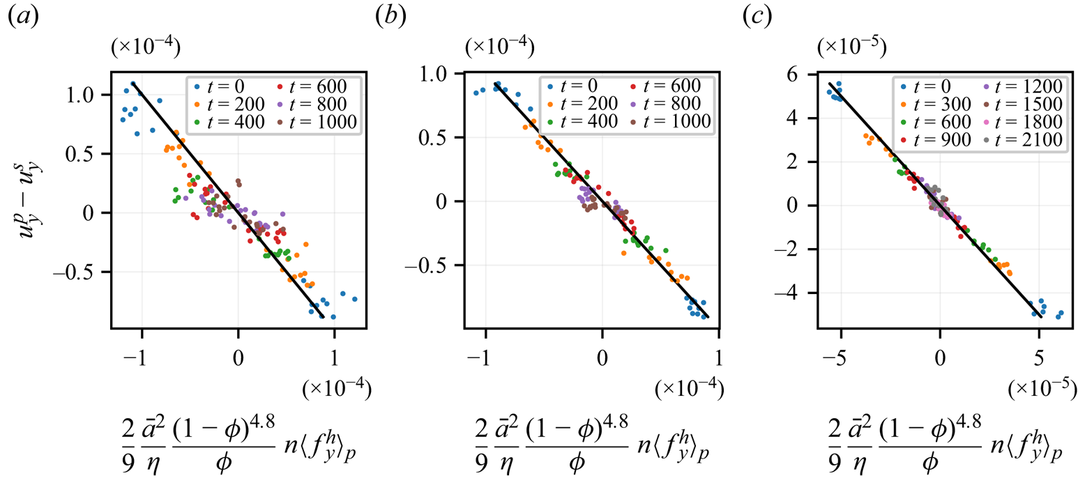
For all simulations, the transverse velocity obeys (3.13) with reasonable accuracy, especially for  $\bar {\phi }=0.4$ and
 $\bar {\phi }=0.5$. In the case
 $\bar {\phi }=0.3$, and to a lesser extent
 $\bar {\phi }=0.4$, a significant discrepancy is observed. It turns out that, at large times, the velocity goes faster towards zero than predicted from the driving force using (3.13). In other words, at the end of the transient flow, a force remains with no particle velocity, equivalent to a small non-drag force. This will be confirmed in the next section, which is dedicated to the steady flow.
Since some stress constitutive laws were shown not to hold in an extended region at the centre of the channel, this particular area deserves specific attention. Figure 23 displays the same quantities as in figure 22, computed from the data in the central region of the channel. Both the velocity and the modified driving force are lower than in the intermediate region, and the data suffer from more noise. However, the same general behaviour as in the intermediate region is observed, which deserves several comments. First, at  $\bar {\phi }=0.5$, the drag law is valid during the whole transient flow, while the volume fraction exceeds
 $\phi _J$ from
 $t = 600$. This suggests that the relation between flux and force is very robust, and hardly depends on the actual suspension microstructure, which is not too surprising, given that Richardson and Zaki correlation primarily applies in particle sedimentation, and is now shown to be valid in shear flow as well. This may be understood given that no long-range order is expected in a sheared suspension, but only preferential orientation of contacting pairs (Blanc et al. Reference Blanc, Lemaire, Meunier and Peters2013), at least for volume fractions not too close to the jamming point. As a consequence, the permeability of such a sheared suspension is expected to be close to that of a random suspension. Second, it should be noted that, at a large time, the force peaks at
 $\bar {\phi }=0.3$ and
 $\bar {\phi }=0.4$, which constitute most of the central region, contributing to the non-drag force. This will be confirmed in the next section.
Transverse relative particle velocity as a function of hydrodynamic hindering force during transient flow: (a)  $\bar {\phi }=0.3$; (b)
 $\bar {\phi }=0.4$; (c)
 $\bar {\phi }=0.5$. See symbol colours online. Data from the central region only. Plain line is theoretical relation (3.13).
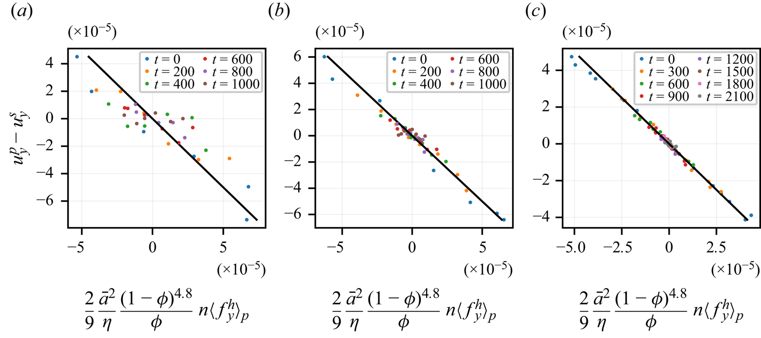
7.3.2. Steady flow
It has been noted in § 6.1.2 that at steady flow the contact and fluid stresses were both uniform across the channel at  $\bar {\phi } = 0.5$, but a gradient of these quantities was observed in the central region in the other cases, and even in the intermediate region at
 $\bar {\phi } = 0.3$. In other words, a finite hydrodynamic force density may occur at some position in the channel while no particle transverse velocity is observed, at odds with the prediction of the standard SBM.
This is well illustrated in figure 24, where the same quantities as in the previous section are displayed for  $\bar {\phi } = 0.3$ and
 $\bar {\phi } = 0.4$. The data at each position in the central and intermediate regions are averaged over the time interval at the end of the simulation, during which the variations of the volume fraction and velocity profiles seem to be insignificant. The specific time interval is quoted in table 1 for each run. The error bars are computed from the standard deviation of each time-averaged quantity, e.g. the particle velocity
 $u^p_y(y)$ at the
 $y$-position in the channel, which is estimated using standard methods (Allen & Tildesley Reference Allen and Tildesley2017; Orsi et al. Reference Orsi, Lobry and Peters2023). In the case of the lowest mean volume fraction
 $\bar {\phi }=0.3$, a small but significant force density persists, while the relative particle velocity vanishes. The data from positions in the central region are highlighted in figure 24, and contribute to this force density. Such a residual force density may be interpreted as a non-drag contribution to the hydrodynamic force. However, it should be noted that in our case, this contribution is quite small compared with the overall force intensity at the beginning of the simulation. At
 $\bar {\phi } = 0.4$, the same trend may be observed, less intense and slightly shadowed by noise. Regarding the velocity that does not appear to vanish exactly in figure 24, it should be kept in mind that the spurious suspension
 $y$-velocity from the solver (§ 7.1) is of the order
 $2\times 10^{-6}$, comparable in magnitude to the velocity displayed in figure 19, and smaller than its standard deviation. Thus, the small remaining velocity seems irrelevant.
Transverse relative particle velocity as a function of hydrodynamic hindering force during steady flow. Data from the intermediate and central regions. The latter is highlighted ( $\square$). Plain line is theoretical relation from (3.13).

Nott et al. (Reference Nott, Guazzelli and Pouliquen2011) argued that the non-drag contribution to the hydrodynamic force could originate in pairwise interaction forces, which would be written as the divergence of stress, the latter built from the particle pair interaction forces in the same way as the contact stress is built from the contact forces ((2.12), (2.13) and (3.6)). The latter relation holds in the case of the subgrid forces, since, from the particular expression of the subgrid resistance matrix (Orsi et al. Reference Orsi, Lobry and Peters2023), it is possible to show that the subgrid stresslet applied on a particle pair is simply the first moment of the subgrid forces on this particle pair, so that
 \begin{equation} \boldsymbol{\nabla} \boldsymbol{\cdot} \boldsymbol{\varSigma} ^{SG} = n \langle\,\boldsymbol{f}^{SG} \rangle _p, \end{equation}
which we have checked in the same way as (3.7) (§ 7.2.1). It is therefore tempting to identify the non-drag force to this pairwise subgrid force, meaning that the drag force density would be the remaining force from the solver  $n \langle \boldsymbol {f}^h \rangle _p^{drag} \approx n \langle \boldsymbol {f}^{FDM} \rangle _p$ while the ‘driving’ force would originate in the short scale pairwise forces
 $n \langle \boldsymbol {f}^{c} + \boldsymbol {f}^{SG} \rangle _p$. This identification cannot have more than a qualitative scope, since the separation between subgrid and solver forces (and stresslets) depends on the computational mesh size. To test this conjecture, the relation between the steady velocity and the steady solver force density is displayed in figure 25. At
 $\bar {\phi } = 0.3$ most of the points are gathered significantly closer to the frame origin than in figure 24, meaning that the solver force density is approximately zero as expected, which seems to confirm the identification of the pairwise subgrid lubrication forces as the source of a non-drag hydrodynamic force. The data from the central region lie further from the theoretical curve, showing that the proposed explanation for the non-drag force seems to fail in this area. At
 $\bar {\phi } = 0.4$, the same argument approximately holds, but the difference between solver and total hydrodynamic forces is less important, due to the weaker relative contribution of the subgrid forces to the normal stress for the considered volume fraction range, as the comparison between figures 21 and 41 (Appendix C) shows. We also note that at
 $\bar {\phi }=0.5$, where the probed volume fraction range is higher, the subgrid forces are relatively even weaker (Appendix C, figure 42), meaning that the non-drag force is approximately zero. Surprisingly, this is also true in the central region, which may be related to the high volume fraction
 $\phi \geq \phi _J$.
Transverse relative particle velocity as a function of solver hydrodynamic hindering force during steady flow. Data from the intermediate and central regions. The latter is highlighted ( $\square$). Plain line is theoretical relation from (3.13).

Finally, as mentioned in § 5.1, while the overall migration is complete during what we call the steady flow, segregation is not, and particle reorganization is still occurring. However, we do not present extensive curves for the segregation dynamics since the data suffers a larger amount of noise, possibly due to the smaller number of particles that constitute each population.
7.4. The SBM migration predictions
For the sake of completeness, the predictions of the SBM are now shortly compared with the simulation data. The governing equations are recalled in Appendix D. They are based on (3.16)–(3.18), without any non-drag force. In addition, to prevent the volume fraction from exceeding the jamming volume fraction, the particle flux is forced to vanish as  $\phi _J$ is reached (Snook et al. Reference Snook, Butler and Guazzelli2016; Badia et al. Reference Badia, D'Angelo, Peters and Lobry2022). This procedure allows carrying out the computations, but obviously cannot account for the large volume fraction observed at the channel centre in the simulations. A specific modelling would be required for this purpose, which we keep for a future study.
The predictions of the SBM are compared with the simulation data in figures 26 and 27 for the mean volume fraction  $\bar {\phi } = 0.4$ and their counterparts for
 $\bar {\phi } = 0.3$ and
 $\bar {\phi } = 0.5$ are displayed in Appendix D.2. The profiles from the SBM have been obtained at a high spatial sampling rate (i.e.
 $\Delta y =0.2 a_1$) and then resampled down to the simulation profiles rate (i.e.
 $\Delta y =a_1$) in the same spirit as the averaging procedure in (4.2). This results in the spreading of the central peak, whose initial growth rate is decreased with respect to the raw profiles. Thanks to this procedure, no peak narrower than a particle radius is observed, in agreement with physical intuition.
Evolution of the (a,b) volume fraction and (c,d) suspension velocity profiles as a function of the mean accumulated strain  $\bar {\gamma }$;
 $\bar {\phi } = 0.4$. The profiles are averaged over a strain interval equal to half the strain sampling period: (a,c) FDM data; (b,d) SBM predictions.

Evolution of (a) volume fraction and (b) suspension velocity as a function of mean accumulated strain at various positions in the channel;  $\bar {\phi } = 0.4$. A running average has been applied to the data to get rid of the high-frequency fluctuations. Plain line is FDM data and the dashed line is SBM predictions.

A fair agreement is found between the simulation data and the SBM predictions, despite significant fluctuations in the former, due to the finite size of the simulation volume. This reflects the good agreement of the simulation data and the main constitutive laws involved in the SBM, at least in the intermediate region. A point-to-point comparison is not easy due to the quite significant volume fraction dispersion at  $\bar {\gamma }=0$ that is sometimes observed, reflecting the mentioned fluctuations. For instance, in the case
 $\bar \phi = 0.4$ (figure 27),
 $\phi (\bar {\gamma }=0)$ extends over the range [0.39, 0.45]. In addition, in the layering area at the boundaries, the volume fraction and the velocity profiles do not match to the SBM prediction, since the main stress constitutive laws are not fulfilled, and the simulated coarse-grained volume fraction is smaller than predicted, as usually observed. In the central region, again, the volume fraction from the simulations either exceeds the jamming volume fraction (
 $\bar {\phi }=0.4$ and
 $0.5$), or does not reach it (
 $\bar {\phi }=0.3$), which has implications on the volume fraction – and velocity – profiles over the whole channel, making the detailed comparison difficult. On the other hand, the SBM predicts a very fine peak at the channel centre that develops very quickly. Such a peak, when it is narrower than the particle size, may not have a clear signification. The resampling procedure that was adopted aims at smoothing out this feature, but does not manage to do so in the most concentrated case (Appendix D.2, figure 45a,b), where the volume fraction at the channel centre as predicted by the SBM evolves faster than measured in the simulation.
Despite these issues, the overall migration dynamics are satisfactorily predicted by the SBM in the intermediate region between the layering area and the channel centre. However, we stress that such comparison yields far less precise information than the local computation of constitutive laws presented before, since the volume fraction and the velocity at a given position are affected by their counterpart at each position in the channel and for all earlier times.
8. Conclusion
In this article, the FDM has been used to simulate the pressure-driven channel flow of non-Brownian suspensions to test, in the particular case of this heterogeneous flow, the validity of various equations and constitutive laws which together form the SBM. Three different values of the mean volume fraction  $\bar {\phi } \in [0.3,\, 0.4,\, 0.5]$ have been investigated. All quantities, e.g. the volume fraction, various velocities and stresses, have been defined as space and time locally averaged variables. Migration is evidenced, together with significant segregation. Despite the latter, the volume fraction varies smoothly across the channel, except for a layering area close to the bounding walls.
As a preliminary check, the usual momentum balance equations for the homogenized suspension have been shown to accurately hold over the whole channel, except close to the bounding walls, where all quantities strongly vary at the particle scale, due to particle layering. This good mechanical behaviour allows us to tackle the rest of the study with confidence.
Leaving aside the layering area, two regions in the flow may be defined, based on the observed rheological laws: an intermediate region between the layering area and the channel centre, where the rheological quantities mostly obey the usual constitutive laws, and a central region, where some discrepancies are observed, pointing to the need for some additional investigations. These two regions have already been evidenced in the past (Yeo & Maxey Reference Yeo and Maxey2011).
In the intermediate region, the stresses have been shown to obey the same constitutive laws as in HSF. We stress that the material functions have been measured using the same numerical method in HSF and channel flow. The local relative shear viscosity and the reduced normal stresses depend on the local volume fraction, or equivalently the local volume fraction and macroscopic friction coefficient  $\mu$ only depend on the local viscous number
 $J$. The quite significant particle segregation is shown to have limited influence on the constitutive laws, in agreement with previous studies from the literature.
The force densities of interest have also been examined. The contact force density, or equivalently the divergence of the contact stress, pushes the particles towards the centre of the channel, while the hydrodynamic force density hinders this motion. In this particular type of flow, where no external force is applied to the particles in addition to the contact and hydrodynamic forces, the hydrodynamic force density is the divergence of the hydrodynamic stress  $\partial _y\varSigma _{yy}^h$. We note that this relation between force density and stress divergence holds over the whole channel. The hydrodynamic stress mostly originates in the fluid solver contribution at the beginning of migration, with a large contribution to the fluid pressure. This feature contributes to highlighting the importance of the pore pressure in the momentum balance of the particle phase (Guazzelli & Pouliquen Reference Guazzelli and Pouliquen2018), and more generally in the transient transport of particles (Marzougui et al. Reference Marzougui, Chareyre and Chauchat2015).
Finally, the relation between the hydrodynamic force density applied to the particles and the particle flux density has been evidenced as well. The hydrodynamic force density obeys the Richardson and Zaki correlation with very good accuracy. However, discrepancies occur in the low volume fraction range, where the force density remains finite while the particle flux vanishes at steady flow. This weak non-drag force might originate in the lubrication forces between close particles, as proposed in the literature (Nott et al. Reference Nott, Guazzelli and Pouliquen2011).
In the central region, some observed flow features strongly contrast with the usual HSF behaviour. The first important result is that the local volume fraction may exceed the jamming volume fraction  $\phi _J$ as computed from HSF simulations, and reach
 $0.65$, i.e. approximately the random close packing fraction, over a central width that is significantly larger than the particle radius, at least in the case of the largest mean volume fraction. This is in agreement with experimental measurements from the literature (Oh et al. Reference Oh, Song, Garagash, Lecampion and Desroches2015). In such a plug region, the suspension is not completely frozen, and a relative motion of the particles is observed, together with a very slow shear. However, the shear rate fluctuations are larger than the mean shear rate, suggesting that the particle motion differs from that observed in a standard shear flow.
Regarding the stress constitutive laws, discrepancies are observed in the central region and are not limited to the area where  $\phi$ exceeds
 $\phi _J$. The relative shear viscosity
 $\eta _S$ is smaller than expected, as is the reduced contact shear stress
 $\hat {\varSigma }_{xy}^c$, while the reduced contact normal stresses are approximately unchanged, except at the very centre of the channel (
 $\kern0.07em y< a_1$) or where
 $\phi \geq \phi _J$. Regarding the
 $\mu (J)$ rheology,
 $\mu$ is lower than expected in the central region and goes to zero instead of the usual finite value (
 $\approx 0.3$) as
 $J$ goes to zero. The suspension microstructure is thus expected to be quite different from the usual HSF shear-induced microstructure. The observed larger shear rate fluctuations in this region support the idea of a non-local contribution to the stress, involving for instance the velocity fluctuations (Gillissen & Ness Reference Gillissen and Ness2020; Bhowmik & Ness Reference Bhowmik and Ness2024). This issue deserves specific work, and we leave it to future studies.
As to the relation between particle flux and hydrodynamic force density, a stronger non-drag force is observed in the central region, which mostly originates in the solver contribution, and seems not to be connected with short-range lubrication forces.
Finally, the FDM has proven to be a powerful and reliable tool for the simulation of moderately to highly concentrated suspensions in heterogeneous flows. In the particular case of a pressure-driven flow, it allowed to locally probe the relevant constitutive laws that define the various stresses and to address the transverse particle flux responsible for migration. In the future, it should help shed light on other issues involving heterogeneous flows, such as particle resuspension.
Acknowledgements
The authors are pleased to thank A. Howard for discussions and for providing the FCM simulation data, and to acknowledge S. Gallier for discussions. They warmly thank M. Antoine for her technical help with the high-performance computing facilities.
Funding
This work was supported by the French National Agency (ANR) under the program Blanc AMARHEO (ANR-18-CE06-0009-01). This work was also supported by the French government through the France 2030 investment plan managed by the National Research Agency (ANR), as part of the Initiative of Excellence Université Côte d'Azur under reference number ANR-15-IDEX-01. The authors are grateful to the Université Côte d'Azur's Centre for High-Performance Computing (OPAL infrastructure) for providing resources and support.
Declaration of interests
The authors report no conflict of interest.
Appendix A. Stress profiles
A.1. Tangential stress profiles
The tangeantial stress profiles for the values of the mean volume fraction  $\overline{\phi} = 0.3$ and
 $0.5$ are displayed in figures 28 and 29.
(a) Steady tangential stress profile, together with contributions detailed in (6.1). (b) Corresponding force densities;  $\bar {\phi }= 0.3$.

(a) Steady tangential stress profile, together with contributions detailed in (6.1). (b) Corresponding force densities;  $\bar {\phi }= 0.5$.
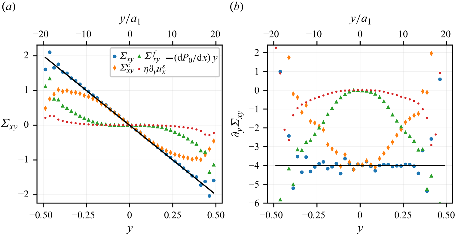
A.2. Normal stress profiles
The normal stress profiles for the values of the mean volume fraction  $\overline{\phi} = 0.3$ and
 $0.5$ are displayed in figures 30 and 31.
Total stress profile (a) together with fluid (b) and contact (c) contributions, at the beginning of the simulation and during steady flow;  $\bar {\phi } =0.3$.
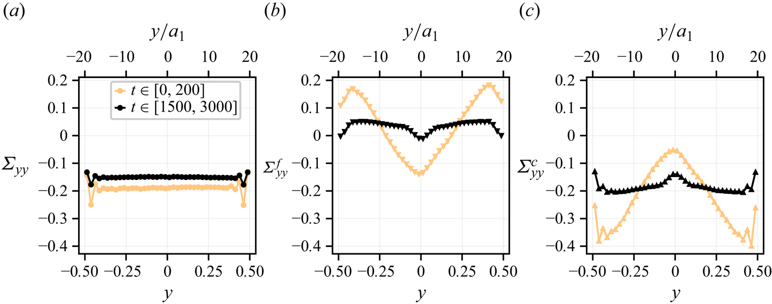
Total stress profile (a) together with fluid (b) and contact (c) contributions, at the beginning of the simulation and during steady flow;  $\bar {\phi } =0.5$.

Appendix B. Material functions
B.1. Shear viscosity
The shear viscosity is displayed as a function of the volume fraction for all 3 values of the mean volume fraction in figure 32.
Shear viscosity as a function of local volume fraction: (a)  $\bar {\phi }=0.3$; (b)
 $\bar {\phi }=0.4$; (c)
 $\bar {\phi }=0.5$. Plain line is (6.3) with
 $\phi _J = 0.592$ and
 $\alpha = 0.8$.
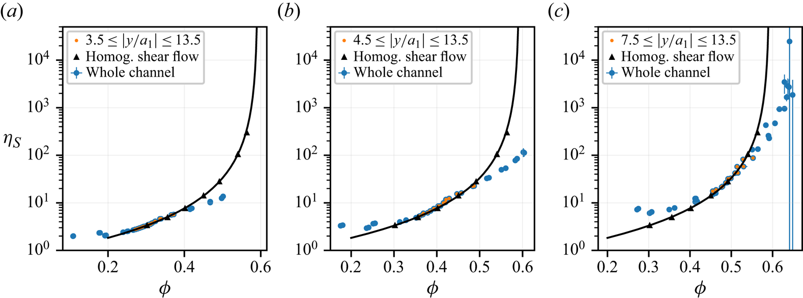
B.2. Normal stress differences
The normal stress differences (4.9a,b) are displayed as a function of the volume fraction for all 3 values of the mean volume fraction in figures 33 and 34.
First normal stress difference as a function of local volume fraction: (a)  $\bar {\phi }=0.3$; (b)
 $\bar {\phi }=0.4$; (c)
 $\bar {\phi }=0.5$. Plain line is correlation law by Badia et al. (Reference Badia, D'Angelo, Peters and Lobry2022).

Second normal stress difference as a function of local volume fraction: (a)  $\bar {\phi }=0.3$; (b)
 $\bar {\phi }=0.4$; (c)
 $\bar {\phi }=0.5$. Plain line is correlation law by Badia et al. (Reference Badia, D'Angelo, Peters and Lobry2022).
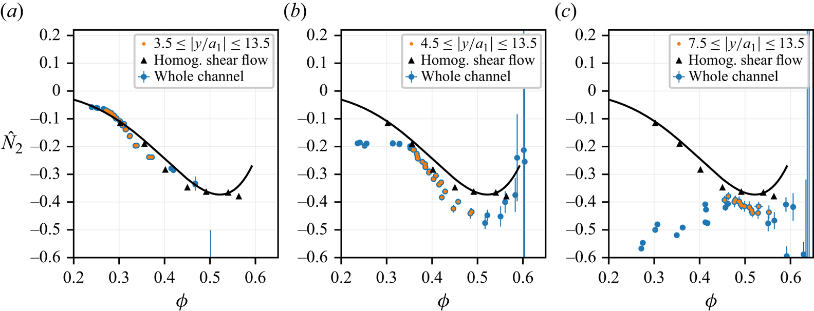
B.3. Reduced contact shear stress
The reduced contact shear stress (4.10a) is displayed as a function of the volume fraction for all 3 values of the mean volume fraction in figure 35.
Reduced contact shear stress as a function of local volume fraction: (a)  $\bar {\phi }=0.3$; (b)
 $\bar {\phi }=0.4$; (c)
 $\bar {\phi }=0.5$. Plain line is correlation law by Badia et al. (Reference Badia, D'Angelo, Peters and Lobry2022).

B.4. Reduced contact normal stresses
The reduced contact normal stresses (4.10b–d) are displayed as a function of the volume fraction for all 3 values of the mean volume fraction in figures 36 to 38.
Reduced contact first normal stress as a function of local volume fraction: (a)  $\bar {\phi }=0.3$; (b)
 $\bar {\phi }=0.4$; (c)
 $\bar {\phi }=0.5$. Plain line is correlation law by Badia et al. (Reference Badia, D'Angelo, Peters and Lobry2022).

Reduced contact second normal stress as a function of local volume fraction: (a)  $\bar {\phi }=0.3$; (b)
 $\bar {\phi }=0.4$; (c)
 $\bar {\phi }=0.5$. Plain line is correlation law by Badia et al. (Reference Badia, D'Angelo, Peters and Lobry2022).
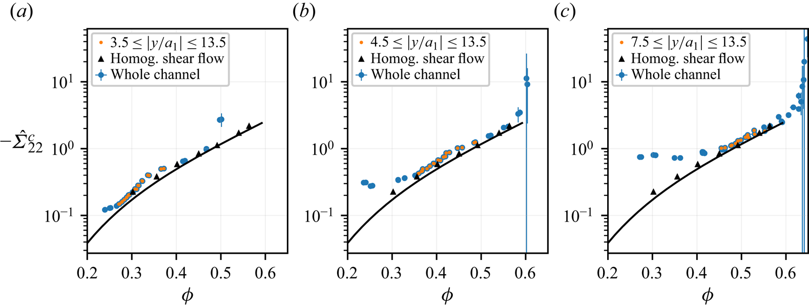
Reduced contact third normal stress as a function of local volume fraction: (a)  $\bar {\phi }=0.3$; (b)
 $\bar {\phi }=0.4$; (c)
 $\bar {\phi }=0.5$. Plain line is correlation law by Badia et al. (Reference Badia, D'Angelo, Peters and Lobry2022).

B.5. The $\mu (J)$ rheology

The flow curve  $\mu(J)$ and
 $\phi(J)$ (4.11a,b) are displayed for all 3 values of the mean volume fraction in figures 39 and 40.
Local macroscopic friction coefficient  $\mu$ as a function of local viscous number
 $J$. Plain line is correlation by Badia et al. (Reference Badia, D'Angelo, Peters and Lobry2022). Dashed line is correlation by Boyer et al. (Reference Boyer, Guazzelli and Pouliquen2011).

Local volume fraction  $\phi$ as a function of local viscous number
 $J$. Plain line is correlation by Badia et al. (Reference Badia, D'Angelo, Peters and Lobry2022). Dashed line is correlation by Boyer et al. (Reference Boyer, Guazzelli and Pouliquen2011).
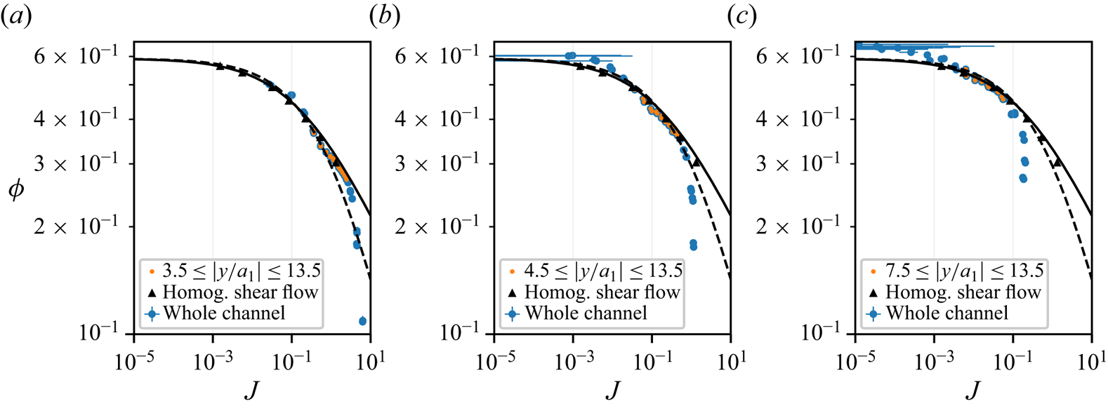
Appendix C. Contributions to the fluid normal stress
Figures 41 and 42 display the contributions to the fluid normal stress  $\Sigma_{22}^f$ (3.10) at the beginning of the simulation run (a) and in steady flow (b) for the values of the mean volume fraction
 $\overline{\phi}=0.3$ and
 $0.5$.
Contributions to the fluid normal stress  $\varSigma _{{22}}^f$ (a) time-averaged stress
 $t \in [0,\, 200]$. (b) Steady profiles
 $t\in [1500,\, 3000]$;
 $\bar {\phi } = 0.3$.

Contributions to the fluid normal stress  $\varSigma _{{22}}^f$ (a) time-averaged stress
 $t \in [0,\, 200]$. (b) Steady profiles
 $t\in [2400,\, 3000]$;
 $\bar {\phi } = 0.5$.
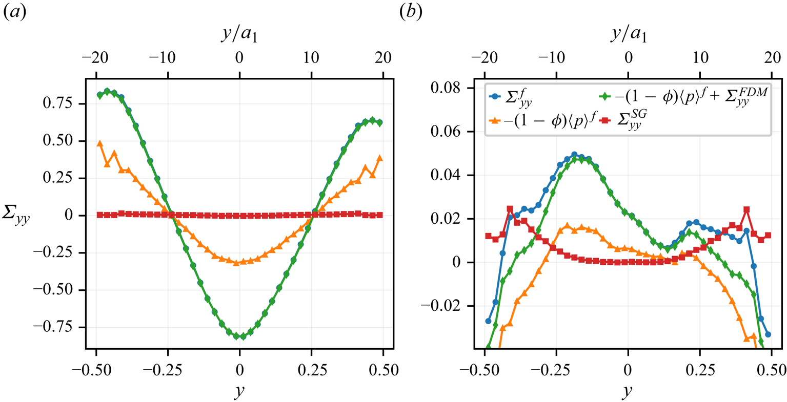
Appendix D. Transient SBM predictions
D.1. Governing equations
In the present section, the equations of the SBM are solved during the same transient plane pressure-driven flow as in the simulations. Due to the imposed constant pressure gradient in the  $x$ direction
 $\boldsymbol \nabla P_0=\textrm {d}P_0/{\textrm {d}\kern0.07em x} \boldsymbol {e}_x$ together with the periodic boundary conditions applied in the
 $x$ and
 $z$ directions, the suspension velocity and volume fraction only depend on
 $y$-coordinate and time
 $t$:
 \begin{equation} \left.\begin{gathered} \boldsymbol{u}_s = u(y,t) \boldsymbol{e}_x,\\ \phi = \phi(y,t). \end{gathered}\right\} \end{equation}
The general transient governing equations, (3.16)–(3.18), have been derived in the Supplementary material section in Orsi et al. (Reference Orsi, Lobry and Peters2023). They are shortly recalled here. The non-drag hydrodynamic forces are neglected, and the following equations have to be solved:
 $$\begin{gather} \varSigma_{xy}=\eta\eta_S(\phi)\dfrac{\partial u}{\partial y} = \dfrac{\mathrm{d}P_0}{\mathrm{d}\kern0.07em x}y , \end{gather}$$
 $$\begin{gather}\dfrac{\partial \phi}{\partial t} + \dfrac{2 \bar a^2}{9 \eta}\dfrac{\partial}{\partial y}\left( f(\phi) \dfrac{\partial}{\partial y}\left( \left\vert\dfrac{\mathrm{d}P_0}{\mathrm{d}\kern0.07em x}\right\vert \vert y \vert \hat \varSigma_{22}^c \right) \right)=0 , \end{gather}$$
where the total tangential stress and the normal contact stress in the  $y$ direction have been written according to (4.8) and (4.10), i.e.
 $$\begin{gather} \varSigma_{xy} = \eta_S(\phi) \eta \dfrac{\partial u}{\partial y}, \end{gather}$$
 $$\begin{gather}\varSigma_{yy}^c =\vert \varSigma_{xy}\vert\hat \varSigma_{22}^c(\phi). \end{gather}$$
The relative shear viscosity has been fitted onto the HSF simulation data from the present article, (6.3),
 \begin{equation} \eta_{s}=\dfrac{\alpha}{\left(1-\dfrac{\phi}{\phi_{J}}\right)^{2}}, \end{equation}
with  $\alpha = 0.8031$ and
 $\phi _J = 0.592$. As to the normal contact stress function, we use the correlation laws from Badia et al. (Reference Badia, D'Angelo, Peters and Lobry2022), which has been shown to satisfactorily fit to the present HSF simulations, and to the pressure driven flow simulations in the intermediate region,
 \begin{equation} \hat{\varSigma}_{22}^{c}(\phi)=d_{1}\left(\frac{\phi}{\phi_{J}}\right)^{d_{2}} \left(e_{1}+e_{2}\frac{\phi}{\phi_{J}}+e_{3}\left(\frac{\phi}{\phi_{J}}\right)^{2}\right), \end{equation}
with  $d_{1}=-2.4247$,
 $d_{2}=4.128$,
 $e_{1}=2.1446$,
 $e_{2}=-2.7234$ and
 $e_{3}=1.5759$.
Finally, the hindered settling function is given the expression that was found to well describe the simulation data, (3.14) with  $n=4.8$,
 \begin{equation} f(\phi)=(1-\phi)^{4.8}. \end{equation}
Boundary conditions are applied at the wall, i.e. a no-slip condition for the velocity, and a vanishing flux condition for the mass balance equation,
 $$\begin{gather} u_{y ={\pm} L_{y}/2} = 0, \end{gather}$$
 $$\begin{gather}J_{y ={\pm} L_{y}/2} = f(\phi) \dfrac{\partial}{\partial y}\left( \left\vert\dfrac{\mathrm{d}P_0}{\mathrm{d}\kern0.07em x}\right\vert \vert y \vert \hat \varSigma_{22}^c \right) = 0. \end{gather}$$
The expression of the flux in (D7b) deserves a few words. As noted, many times (Miller & Morris Reference Miller and Morris2006; Snook et al. Reference Snook, Butler and Guazzelli2016; Badia et al. Reference Badia, D'Angelo, Peters and Lobry2022), it cannot prevent the volume fraction exceeding the jamming volume fraction at the channel centre plane. It is possible to circumvent this difficulty by arbitrarily forcing the flux to vanish as the jamming volume fraction is reached, allowing us to carry out the computation. Obviously, this expedient does not yield a volume fraction larger than the jamming volume fraction, and the computation does not agree with the simulations in that aspect. Specific modelling should be developed to this purpose, which we find out of the scope of the present study.
Equations (D2a) and (D2b) are made dimensionless in the same way as in § 2.3:
 $$\begin{gather} \dfrac{\partial u}{\partial y} ={-}4\dfrac{y}{\eta_S(\phi)}, \end{gather}$$
 $$\begin{gather}\dfrac{\partial \phi}{\partial t} + \dfrac{8 }{9}\bar a^2\dfrac{\partial}{\partial y}\left( f(\phi) \dfrac{\partial}{\partial y}(\vert y \vert \hat \varSigma_{22}^c) \right)=0 , \end{gather}$$
where all quantities are now dimensionless.
D.2. The SBM predictions
The SBM predictions for the suspension volume fraction and velocity from the equations above are compared with the results from the FDM computations in the figures below, for the values of the mean volume fraction  $\overline{\phi} = 0.3$ (figures 43 and 44) and
 $\overline{\phi}= 0.5$ (figures 45 and 46).
Evolution of the (a,b) volume fraction and (c,d) suspension velocity profiles as a function of the mean accumulated strain  $\bar {\gamma }$;
 $\bar {\phi } = 0.3$. The profiles are averaged over a strain interval equal to half the strain sampling period: (a,c) FDM data; (b,d) SBM predictions.
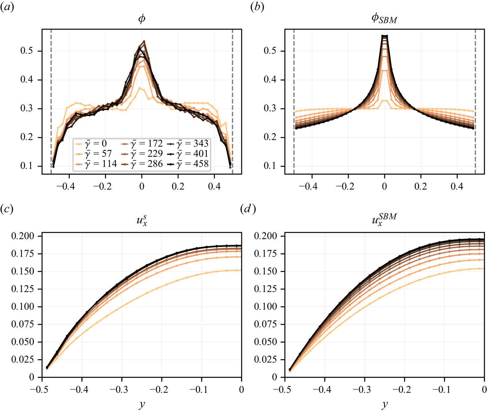
Evolution of (a) volume fraction and (b) suspension velocity as a function of mean accumulated strain at various positions in the channel;  $\bar {\phi } = 0.3$. A running average has been applied to the data in order to get rid of the high frequency fluctuations. Plain line is FDM data; dashed line is SBM predictions.

Evolution of the (a,b) volume fraction and (c,d) suspension velocity profiles as a function of the mean accumulated strain  $\bar {\gamma }$;
 $\bar {\phi } = 0.5$. The profiles are averaged over a strain interval equal to half the strain sampling period: (a,c) FDM data; (b,d) SBM predictions.

Evolution of (a) volume fraction and (b) suspension velocity as a function of mean accumulated strain at various positions in the channel;  $\bar {\phi } = 0.5$. A running average has been applied to the data in order to get rid of the high frequency fluctuations. Plain line is FDM data and the dashed line is SBM predictions.