1 Introduction
We consider an axisymmetric viscous thread that is pulled from both ends at a prescribed speed that, in general, varies with time. This type of flow is found in a range of industrial applications such as the drawing of glass and polymer fibres for optical microscopy and for glass microelectrodes (DeWynne, Ockendon & Wilmott Reference DeWynne, Ockendon and Wilmott1989; Huang et al. Reference Huang, Miura, Ireland and Puil2003, Reference Huang, Wylie, Miura and Howell2007). It is also applicable to measurement of extensional viscosity by stretching of a liquid bridge, as commonly used for non-Newtonian fluids (Matta & Titus Reference Matta and Titus1990; Sridhar et al. Reference Sridhar, Tirtaatmadja, Nguyenand and Gupta1991; Berg, Kröger & Rath Reference Berg, Kröger and Rath1994; Gaudet, McKinley & Stone Reference Gaudet, McKinley and Stone1996; Spiegelberg, Ables & McKinley Reference Spiegelberg, Ables and McKinley1996; Yao & McKinley Reference Yao and McKinley1998; Berg, Dreyer & Rath Reference Berg, Dreyer and Rath1999; Olagunju Reference Olagunju1999).
An extensive literature exists on the extensional flow of thin viscous jets and threads under various conditions, and one-dimensional models, along with numerical simulation and experiments, are commonly used to investigate them. Eggers (Reference Eggers2005) and Eggers & Villermaux (Reference Eggers and Villermaux2008) provide a good overview of the area.
In the absence of external stretching and inertia, a number of authors have considered the stability and break up of slender axisymmetric threads and jets. Linear stability theory was pioneered by Rayleigh (Reference Rayleigh1879, Reference Rayleigh1892) but progress on the mathematical description of nonlinear effects came a century later with the use of similarity methods. In ground breaking work Eggers (Reference Eggers1993) found a universal similarity solution that describes break up of axisymmetric Newtonian threads, which is independent of the initial conditions. Other transient similarity solutions for uniform axisymmetric Newtonian cylinders were found in the limits of high viscosity (Papageorgiou Reference Papageorgiou1995) and low viscosity (Chen & Steen Reference Chen and Steen1997; Day, Hinch & Lister Reference Day, Hinch and Lister1998) but ultimately it is the universal solution that describes the break up. As far as we are aware, the role of initial conditions in break up was first examined by Renardy (Reference Renardy1994) for a uniform axisymmetric fluid cylinder by solving the long-wavelength equations written in terms of standard Lagrangian coordinates. He considered both Newtonian and a number of non-Newtonian fluids with the aim of explaining why non-Newtonian fluid threads are typically more stable than those of Newtonian fluids and, indeed, may not break up at all. Further work using a combination of asymptotic and numerical methods is reported in Renardy (Reference Renardy1995). Similarity solutions for various viscoelastic fluid models followed (Renardy Reference Renardy2002) and an extensive review of self-similar break up is contained in Renardy (Reference Renardy, Binding and Walters2004). Additional asymptotic and numerical analysis can be found in Fontelos & Li (Reference Fontelos and Li2004).
In this paper, we consider a problem in which the fluid thread is subject to external stretching. Such problems have also received considerable attention. For Newtonian threads near break up, the universal solution of Eggers (Reference Eggers1993) is also relevant. However, in order to find the time and location of the pinching point, both the initial geometry and boundary conditions must be taken into account, which poses a number of challenges. We directly address this question for the case of an axisymmetric viscous Newtonian thread that is pulled from both ends with a prescribed speed such that inertia is initially negligible. We determine conditions on the pulling speed such that inertia will remain negligible indefinitely. If the pulling speed is such that inertia becomes important, we derive long-time asymptotic solutions and show that there are a number of generic cases that exhibit markedly different behaviour.
Whilst some authors have solved similar extensional flow problems by numerical simulation (Yao & McKinley Reference Yao and McKinley1998; Wilkes, Phillips & Basaran Reference Wilkes, Phillips and Basaran1999), much can be learned from simplified models that exploit the slenderness of the thread. Matovich & Pearson (Reference Matovich and Pearson1969) and DeWynne, Ockendon & Wilmott (Reference DeWynne, Ockendon and Wilmott1992) formally derived the appropriate long-wavelength equations to model the extensional flow of long thin Newtonian threads which have since been used by many authors. Kaye (Reference Kaye1991) and Renardy (Reference Renardy1994) derived the equations with a general constitutive law for the study of non-Newtonian fluid threads. Wilson (Reference Wilson1988) and Stokes, Tuck & Schwartz (Reference Stokes, Tuck and Schwartz2000) studied the slender initial boundary value problem for a viscous Newtonian drop elongating under gravity when inertia is negligible; the role of inertia in the problem was examined by Stokes & Tuck (Reference Stokes and Tuck2004). By numerically solving long-wavelength equations, gravitational extension of slender viscoplastic fluid threads has also been studied, both neglecting (Al Khatib Reference Al Khatib2003) and including (Balmforth, Dubashi & Slim Reference Balmforth, Dubashi and Slim2010) inertia and surface tension. For a liquid bridge that is pulled from one or both ends, the zero-inertia leading-order long-wavelength solution (that is an ideal uniaxial elongational flow) has been compared with full numerical solutions (Yao & McKinley Reference Yao and McKinley1998) and with experiments (Spiegelberg et al. Reference Spiegelberg, Ables and McKinley1996) for Newtonian and non-Newtonian fluids. Long-wavelength models for liquid bridges of various non-Newtonian fluids have been solved numerically by Olagunju (Reference Olagunju1999) and Balmforth et al. (Reference Balmforth, Dubashi and Slim2010), with the latter authors including experimental comparisons. Such problems have also received attention in the context of the drawing of Newtonian fibres (Gupta & Schultz Reference Gupta and Schultz1998; Forest, Zhou & Wang Reference Forest, Zhou and Wang2000; Yin & Jaluria Reference Yin and Jaluria2000; Fitt et al. Reference Fitt, Furusawa, Monro and Please2001).
Lastly we mention that long-wavelength models have been used for filaments subject to a constant pulling force. Kaye (Reference Kaye1991) included gravity and solved the problem with weak inertial effects, but did not examine the case in which inertia becomes significant. Huang et al. (Reference Huang, Miura, Ireland and Puil2003, Reference Huang, Wylie, Miura and Howell2007) discussed the pulling of externally heated glass tubes in the case in which inertia is negligible. The importance of viscous heating and inertia when threads become highly extended is discussed in Wylie & Huang (Reference Wylie and Huang2007).
Previous authors have shown that there are a number of advantages in using a Lagrangian coordinate as the independent variable for extensional flow problems and, where numerical solution is necessary, have designed Lagrangian-based numerical methods. However, in regions where the thread becomes sufficiently extended, such methods do not adequately resolve the solution. In Bradshaw-Hajek, Stokes & Tuck (Reference Bradshaw-Hajek, Stokes and Tuck2007), the gravitational extension of a fluid drop was studied using a novel formulation with the Lagrangian coordinate as the dependent variable and a numerical technique that provides good numerical resolution in the filament region. The same formulation is used here but with a non-standard Lagrangian coordinate.
Whether the radius of the thread can become zero in a finite time when surface tension is neglected is a topic of interest. It has been previously shown that this occurs for a thread extending under gravity or a constant force with zero inertia, but does not occur with finite inertia (Wilson Reference Wilson1988; Stokes et al. Reference Stokes, Tuck and Schwartz2000; Stokes & Tuck Reference Stokes and Tuck2004; Wylie, Huang & Miura Reference Wylie, Huang and Miura2011). On the other hand, for a thread whose ends are extended at a controlled velocity, no such finite-time singularity occurs even when inertia is neglected (Hassager, Kolte & Renardy Reference Hassager, Kolte and Renardy1998). In this paper, we consider extension with a controlled velocity and include inertia. Therefore, when surface tension is neglected, a finite-time singularity will not occur.
In a previous paper, Wylie et al. (Reference Wylie, Huang and Miura2011) examined a viscous, axisymmetric thread extending under the influence of a constant force for small initial surface tension and inertial effects. Surface tension was shown to remain negligible, while inertia was shown to ultimately become important. As a result, the thinning of the thread is eventually dominated by the dynamics at the pulled end and pinching must occur there. In the problem we study in this paper, the thread is pulled from both ends with a prescribed speed. In this case, we uncover a number of different types of behaviour and the mechanics and mathematical techniques are very different from the constant force case.
In this paper, we first formulate the problem in a particularly convenient form. We then examine the small-inertia case and show that the problem under consideration naturally splits into two generic cases. The first has an initial minimum cross-sectional area at the pulled ends, whilst the second has an initial minimum away from the pulled ends. As representative of this second case, we choose an initial shape which has its minimum at the point of symmetry in the centre of the thread. As a third case, we consider an initially cylindrical thread which, although a non-generic special case, exhibits different behaviour and is of interest in practical applications. For each of these cases, we examine the evolution of the thread shape when inertia is small, finding asymptotic expressions which compare well with numerical solutions. Using this analysis, we determine the conditions on pulling speed such that inertia remains negligible indefinitely. We also show that these conditions on the speed are different for the two generic initial shapes. In the cases where the pulling speed is such that inertia ultimately becomes important, we determine the large-time behaviour for each type of initial thread shape. Moreover, if the initial minimum is not at the pulled end, we show that there are two very different types of solution that exhibit very different extension mechanics. In addition, we compare both the small-inertia and large-time solutions with numerical solutions. Despite the fact that this is an essentially diffusive problem, we show that there may be regions of the flow where the effects of the initial conditions do not decay rapidly enough that they can be ignored. That is, there are cases for which the initial geometry of the thread affects the leading-order solution indefinitely.
2 Formulation
Consider an axisymmetric thread composed of a viscous fluid whose viscosity, density and surface tension coefficient are assumed to be constant and given by
 ${\it\mu}$
,
 ${\it\rho}$
and
 ${\it\gamma}$
, respectively. We denote the distance measured along the axis of the thread as
 $x$
and the time as
 $t$
. We will assume that the thread initially has zero velocity, half-length
 $L_{0}$
and cross-sectional area
 $A_{0}(x)$
. For simplicity, we will assume that the thread is symmetric about
 $x=0$
, that is
 $A_{0}(x)\equiv A_{0}(-x)$
. The thread is extended by pulling at both ends with a time-dependent speed
 $V(t)$
. The ends of the thread are located at
 $x=\pm L(t)$
, where
 $L(t)$
is the half-length of the thread that satisfies
 $V(t)=\dot{L}(t)$
with initial condition
 $L(0)=L_{0}$
. Here, the dot denotes differentiation with respect to time. In fact, rather than specifying
 $V(t)$
, it proves to be slightly more convenient to specify
 $L(t)$
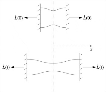
. The configuration of the problem is depicted in figure 1. As far as possible we will formulate and solve the problem for general
 $L(t)$
. However, we have found that functions that have the asymptotic form
 $$\begin{eqnarray}L(t)\sim t^{{\it\alpha}}\quad \text{as}~t\rightarrow \infty ,\end{eqnarray}$$
where
 ${\it\alpha}>0$
, capture the surprisingly rich variety of possible behaviours. For definiteness, we will consider the family of functions
 $L(t)=L_{0}(1+{\it\tau}t)^{{\it\alpha}}$
, where
 ${\it\tau}^{-1}$
is an appropriate time scale for the pulling.
A slender viscous thread is pulled by its ends by a time-dependent speed
 $V(t)=\dot{L}(t)$
, where
 $L(t)$
is the half-length of the thread. The initial shape of the thread is shown in the upper figure, while the shape at a later time
 $t$
is shown in the bottom figure.

2.1 Standard long-wavelength equations
We consider threads with small aspect ratio
 ${\it\epsilon}=\sqrt{A_{min}/({\rm\pi}L_{0}^{2})}\ll 1$
, where
 $A_{min}$
is the initial minimum cross-sectional area. To leading order in
 ${\it\epsilon}$
, it has been shown (Fitt et al.
Reference Fitt, Furusawa, Monro and Please2001) that, the axial fluid velocity,
 $u(x,t)$
, is independent of the radial coordinate and the long-wavelength Navier–Stokes and continuity equations are given by
 $$\begin{eqnarray}\displaystyle \frac{\partial u}{\partial t}+u\displaystyle \frac{\partial u}{\partial x}=\displaystyle -\frac{{\it\gamma}}{{\it\rho}}\displaystyle \frac{\partial }{\partial x}\left(\sqrt{\frac{{\rm\pi}}{A}}\right)+\displaystyle \frac{3{\it\mu}}{{\it\rho}}\frac{1}{A}\displaystyle \frac{\partial }{\partial x}\left(A\displaystyle \frac{\partial u}{\partial x}\right)\end{eqnarray}$$
and
 $$\begin{eqnarray}\frac{\partial A}{\partial t}+\frac{\partial }{\partial x}(uA)=0,\end{eqnarray}$$
respectively. Here,
 $A(x,t)$
is the cross-sectional area that is defined for
 $0\leqslant x\leqslant L(t)$
. Using the symmetry condition at
 $x=0$
, the boundary conditions are given by
 $$\begin{eqnarray}\frac{\partial A}{\partial x}(0,t)=0\quad \text{and}\quad u(L(t),t)=\dot{L}(t).\end{eqnarray}$$
The initial conditions are given by
 $$\begin{eqnarray}A(x,0)=A_{0}(x),\quad u(x,0)=0.\end{eqnarray}$$
We now adopt non-dimensional variables (denoted by bars) defined by
 $$\begin{eqnarray}u={\it\tau}L_{0}\bar{u},\quad A=A_{min}\bar{A},\quad A_{0}=A_{min}\bar{A_{0}},\quad x=L_{0}\bar{x},\quad t={\it\tau}^{-1}\bar{t}.\end{eqnarray}$$
After substituting into the governing equations and dropping the bars, we obtain
 $$\begin{eqnarray}\displaystyle & \displaystyle R\left(\displaystyle \frac{\partial u}{\partial t}+u\displaystyle \frac{\partial u}{\partial x}\right)=-{\it\Gamma}\displaystyle \frac{\partial }{\partial x}\left(\displaystyle \frac{1}{\sqrt{A}}\right)+\displaystyle \frac{1}{A}\frac{\partial }{\partial x}\left(A\frac{\partial u}{\partial x}\right), & \displaystyle\end{eqnarray}$$
 $$\begin{eqnarray}\displaystyle & \displaystyle \frac{\partial A}{\partial t}+\displaystyle \frac{\partial }{\partial x}(uA)=0, & \displaystyle\end{eqnarray}$$
where
 $$\begin{eqnarray}R={\it\rho}{\it\tau}L_{0}^{2}/(3{\it\mu})\end{eqnarray}$$
is the Reynolds number based on the initial length of the thread, and
 $$\begin{eqnarray}{\it\Gamma}=\displaystyle \frac{{\it\gamma}}{3{\it\mu}{\it\tau}}\sqrt{\frac{{\rm\pi}}{A_{min}}}=\frac{{\it\gamma}}{3{\it\mu}{\it\tau}L_{0}{\it\epsilon}}\end{eqnarray}$$
is a dimensionless capillary number that measures the surface tension force relative to the viscous force. Using (2.8), the Navier–Stokes equation (2.7) may be rewritten in the form
 $$\begin{eqnarray}R\frac{\text{D}u}{\text{D}t}=\frac{1}{A}\frac{\partial }{\partial x}\left(-\frac{\text{D}A}{\text{D}t}+{\it\Gamma}\sqrt{A}\right),\end{eqnarray}$$
where
 $$\begin{eqnarray}\frac{\text{D}}{\text{D}t}=\frac{\partial }{\partial t}+u\frac{\partial }{\partial x}\end{eqnarray}$$
denotes the material time derivative. The initial and boundary conditions (2.4)–(2.5) remain unchanged under the non-dimensionalisation. Note that
 $A_{0}(x)\geqslant 1$
since the cross-sectional area is scaled by the minimum cross-sectional area.
We now consider the case
 $R\ll 1$
and
 ${\it\Gamma}\ll 1$
, so that, initially, inertia and surface tension can be neglected. However, we note that the dimensionless estimates of
 $R$
and
 ${\it\Gamma}$
are based on the initial length and cross-sectional area of the thread. If the thread becomes sufficiently thin and heavily extended, it is possible that these estimates do not adequately represent the importance of inertial and surface tension effects. This is the case for a thread pulled by a constant force, for which Wylie et al. (Reference Wylie, Huang and Miura2011) showed that even though
 $R\ll 1$
, inertia must ultimately become important. On the other hand, they were able to use non-trivial asymptotic estimates to show that if
 ${\it\Gamma}\ll 1$
, then surface tension forces remain negligible throughout the entire stretching process. We therefore proceed by setting
 ${\it\Gamma}=0$
. The conditions which justify this assumption are discussed in the closing remarks.
Before continuing, we briefly comment on the nature of the initial conditions. To do this we need to address the question of how, in a physical context, the shape of the thread immediately prior to the stretching process arises. The fluid thread must first be attached to the two ends at which the pulling is applied. Following the attachment process, there may be a period of time before the pulling commences. If this time is sufficiently short compared with the time scale for surface tension to significantly deform the thread, then the shape will remain undeformed by surface tension. On the other hand, if the waiting time is sufficiently long, then surface tension will modify the thread shape until eventually a minimal energy surface is achieved. For materials like polymers or glasses that are effectively solid at room temperature, external heating must be applied until the viscosity of the material decreases sufficiently to allow stretching with reasonable extensional forces. After heating, these materials typically have a viscosity of the order
 $10^{4}~\text{Pa}~\text{s}$
(and possibly many orders of magnitude larger) and surface tension coefficients of order
 $10^{-1}~\text{N}~\text{m}^{-1}$
. Using these estimates and considering threads with radius of order
 $10^{-2}~\text{m}$
, the time scale required for surface tension to modify the shape is of order
 $10^{3}~\text{s}$
. So, as long as the waiting time is limited to a few minutes, surface tension will play a negligible role in determining the initial condition and a wide range of initial shapes are feasible.
2.2 Transformed equations
We now introduce a transformation that significantly simplifies the form of the equations. Following Bradshaw-Hajek et al. (Reference Bradshaw-Hajek, Stokes and Tuck2007), we introduce the variable
 $$\begin{eqnarray}Z(x,t)=\frac{1}{I}\int _{0}^{x}A(x^{\prime },t)\,\text{d}x^{\prime }\quad \text{where}~I=\displaystyle \int _{0}^{1}A_{0}(x^{\prime })\,\text{d}x^{\prime }=\int _{0}^{L(t)}A(x^{\prime },t)\,\text{d}x^{\prime }.\end{eqnarray}$$
Since the thread is symmetric about
 $x=0$
,
 $I$
represents half of the total volume of the fluid (and remains constant throughout the stretching process). The variable
 $Z(x,t)$
is the fraction of the volume between 0 and
 $x$
. Given
 $Z(x,t)$
, one can readily calculate the cross-sectional area
 $A(x,t)$
via
 $$\begin{eqnarray}A=IZ_{x},\end{eqnarray}$$
which is obtained by partially differentiating (2.13a
) with respect to
 $x$
.
Using conservation of mass (2.3), one can readily check that
 $$\begin{eqnarray}\text{D}Z/\text{D}t=Z_{t}+uZ_{x}=0.\end{eqnarray}$$
This shows that
 $Z$
is constant when following any given fluid element. From a physical viewpoint this is completely natural, since the amount of fluid between the symmetry axis
 $x=0$
and a given fluid element must be conserved. In some sense,
 $Z$
can therefore be considered as a Lagrangian variable, although it is important to note that, in terms of the equations we will derive,
 $Z$
will be a dependent, rather than an independent variable. (However, for the asymptotics of § 4.2 it will prove useful to use
 $Z$
as a Lagrangian independent variable.)
Using (2.15), the velocity
 $u$
can be written as
 $$\begin{eqnarray}u=-\frac{Z_{t}}{Z_{x}},\end{eqnarray}$$
where the subscript denotes partial differentiation. Substituting (2.16) and (2.14) into (2.11) with
 ${\it\Gamma}=0$
, we obtain
 $$\begin{eqnarray}R\,\frac{\text{D}}{\text{D}t}\left(\frac{Z_{t}}{Z_{x}}\right)=\frac{1}{Z_{x}}\frac{\partial }{\partial x}\left(\frac{\text{D}}{\text{D}t}(Z_{x})\right).\end{eqnarray}$$
After some straightforward algebra, this can be expressed as
 $$\begin{eqnarray}R\,\frac{\text{D}}{\text{D}t}\left(\frac{Z_{t}}{Z_{x}}\right)=\frac{\text{D}}{\text{D}t}\left(\frac{Z_{xx}}{Z_{x}}\right).\end{eqnarray}$$
Integration of (2.18) with respect to the material time introduces a general function of the Lagrangian variable
 $Z$
. The function is obtained using the initial condition (2.5) and (2.13b
) to give
 $$\begin{eqnarray}RZ_{t}=Z_{xx}-\displaystyle \frac{s_{0}^{\prime }(Z)}{I}Z_{x}=\frac{\partial }{\partial x}\left(Z_{x}-\frac{s_{0}(Z)}{I}\right),\end{eqnarray}$$
where
 $s_{0}(Z)$
is the initial shape of the thread expressed as a function of
 $Z$
. Since
 $Z(x,t)$
is the fraction of the volume between 0 and
 $x$
, the boundary conditions are
 $$\begin{eqnarray}Z(0,t)=0\quad \text{and}\quad Z(L(t),t)=1.\end{eqnarray}$$
We conclude this section with a brief note regarding the relationship between
 $A_{0}(x)$
and
 $s_{0}(Z)$
that represent the initial shape of the thread specified in Eulerian and Lagrangian coordinates, respectively. It is more physically natural to specify
 $A_{0}(x)$
, but since
 $s_{0}(Z)$
appears in the governing equation for
 $Z$
(2.19), for the purpose of analysis, it is often more convenient to specify
 $s_{0}(Z)$
. On the one hand, if
 $A_{0}(x)$
is specified, one can use (2.13) with
 $t=0$
to obtain
 $Z\equiv Z(x)$
. Inverting this function allows us to express
 $x$
as a function of
 $Z$
,
 $x\equiv x(Z)$
. Substituting this into
 $A_{0}(x)$
we obtain
 $s_{0}(Z)$
. On the other hand, if
 $s_{0}(Z)$
is specified, one can calculate
 $I$
from (2.14) with
 $t=0$
, writing
 $1/I=Z_{x}/s_{0}(Z(x))$
and integrating to give
 $$\begin{eqnarray}x(Z)=I\int _{0}^{Z}\frac{1}{s_{0}(Z^{\prime })}\,\text{d}Z^{\prime }.\end{eqnarray}$$
Then, since
 $Z=1$
corresponds to
 $x=1$
at
 $t=0$
, we have
 $$\begin{eqnarray}I=\left[\int _{0}^{1}\frac{1}{s_{0}(Z)}\,\text{d}Z\right]^{-1}.\end{eqnarray}$$
One can then use (2.21) to obtain
 $x\equiv x(Z)$
. Inverting this function allows us to express
 $Z$
as a function of
 $x$
,
 $Z\equiv Z(x)$
. Substituting this into
 $s_{0}(Z)$
we obtain
 $A_{0}(x)$
.
3 Initial stretching with small inertia
We begin by noting that the initial condition (2.5b
) is inconsistent with the boundary condition (2.4b
). This implies that there is an initial temporal adjustment region of width
 $t=O(R)$
over which the solution rapidly adjusts from the initial condition. This adjustment occurs on a time scale much faster than the time scales of interest in this problem and is therefore not of relevance for this study.
At early times of
 $O(1)$
, the Reynolds number is small and, hence, we expand
 $Z(x,t)$
in powers of
 $R$
thus:
 $$\begin{eqnarray}Z(x,t)=Z_{0}(x,t)+RZ_{1}(x,t)+O(R^{2}).\end{eqnarray}$$
Using (2.14), the cross-sectional area is then given by
 $$\begin{eqnarray}\displaystyle A(x,t) & = & \displaystyle IZ_{0x}(x,t)+RIZ_{1x}(x,t)+O(R^{2})\nonumber\\ \displaystyle & = & \displaystyle A_{0}(x,t)+RA_{1}(x,t)+O(R^{2}).\end{eqnarray}$$
Substituting the above expression for
 $Z(x,t)$
into (2.19) and (2.20) gives, at leading order in
 $R$
,
 $$\begin{eqnarray}\partial _{x}\left(Z_{0x}-\frac{s_{0}(Z_{0})}{I}\right)=0,\quad Z_{0}(0,t)=0,\quad Z_{0}(L(t),t)=1,\end{eqnarray}$$
and at first order in
 $R$
,
 $$\begin{eqnarray}Z_{0t}=\partial _{x}\left(Z_{1x}-\frac{s_{0}^{\prime }(Z_{0})Z_{1}}{I}\right),\quad Z_{1}(0,t)=Z_{1}(L(t),t)=0.\end{eqnarray}$$
Integrating (3.3a-c
) with respect to
 $x$
gives
 $$\begin{eqnarray}Z_{0x}-\displaystyle \frac{1}{I}s_{0}(Z_{0})=\frac{1}{I}h(t),\end{eqnarray}$$
where
 $h(t)$
is a function that must be determined using the boundary conditions. Equation (3.5) is separable and after integration and applying the boundary condition
 $Z_{0}(0,t)=0$
, we obtain
 $$\begin{eqnarray}\displaystyle \int _{0}^{Z_{0}}\frac{I}{s_{0}(Z^{\prime })+h(t)}\,\text{d}Z^{\prime }=x.\end{eqnarray}$$
Using the other boundary condition,
 $Z_{0}(L(t),t)=1$
gives
 $$\begin{eqnarray}I\displaystyle \int _{0}^{1}\displaystyle \frac{1}{s_{0}(Z^{\prime })+h(t)}\,\text{d}Z^{\prime }=L(t).\end{eqnarray}$$
For given functions
 $s_{0}(Z)$
and
 $L(t)$
, (3.7) represents an integral equation for the function
 $h(t)$
. After solving for
 $h(t)$
, the leading-order solution
 $Z_{0}(x,t)$
is given by (3.6). This can then be substituted into (3.4) which can then be solved using the boundary conditions to give the first-order correction term
 $Z_{1}(x,t)$
.
As time becomes large,
 $L(t)$
also becomes large, see (2.1). Since
 $I$
is
 $O(1)$
, the denominator of the fraction in the integral in (3.7) must become small at large times. From this, we see that
 $h(t)\rightarrow -\min \,s_{0}(Z)$
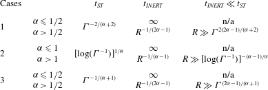
. This suggests consideration of two generic cases. In the first, the initial minimum cross-sectional area of the thread occurs at the pulled end. In the second, the initial minimum cross-sectional area occurs away from the pulled end. We study these two generic cases and, in addition, the special case of an initially cylindrical thread. The analysis for the cylindrical case is simplest and we present this first.
3.1 Case 1: initially cylindrical thread
In this case,
 $s_{0}(Z)=A_{0}(x)=1$
,
 $I=1$
, and
 $Z(x,0)=x$
,
 $0\leqslant x\leqslant 1$
(via (2.13a
)), so that (2.19) reduces to
 $$\begin{eqnarray}RZ_{t}=Z_{xx},\end{eqnarray}$$
to be solved subject to boundary conditions
 $$\begin{eqnarray}Z(0,t)=0\quad \text{and}\quad Z(L(t),t)=1.\end{eqnarray}$$
The leading-order solution satisfies
 $Z_{0xx}=0$
and, using the boundary conditions, we find
 $$\begin{eqnarray}Z_{0}=\frac{x}{L}.\end{eqnarray}$$
Substituting for
 $Z_{0}$
in (3.4) gives
 $$\begin{eqnarray}-\frac{x}{L^{2}}\dot{L}=Z_{1xx},\end{eqnarray}$$
to be solved subject to boundary conditions
 $Z_{1}(0,t)=Z_{1}(L(t),t)=0$
. We find
 $$\begin{eqnarray}Z_{1}=-\frac{{\it\alpha}x\dot{L}}{6L^{2}}[x^{2}-L^{2}].\end{eqnarray}$$
Hence, to first order in
 $R$
, we have the solution
 $$\begin{eqnarray}Z=\displaystyle \frac{x}{L}\left\{1-\displaystyle \frac{R}{6}L\dot{L}\left(\displaystyle \frac{x^{2}}{L^{2}}-1\right)\right\},\end{eqnarray}$$
from which we can find the cross-sectional area,
 $A=IZ_{x}$
.
We must, however, ensure that the series for
 $A$
remains asymptotically valid, i.e. that the second term in the series for
 $Z_{x}$
is smaller than the first. The ratio
 $$\begin{eqnarray}\displaystyle \frac{RA_{1}}{A_{0}}=\displaystyle \frac{RZ_{1x}}{Z_{0x}}\sim RL\dot{L}\left(\displaystyle \frac{3x^{2}}{L^{2}}-1\right)\end{eqnarray}$$
has largest magnitude at the end of the thread (
 $x=L$
), so that in order for the series to remain valid, we require
 $$\begin{eqnarray}RL\dot{L}\ll 1.\end{eqnarray}$$
At early times, this quantity is small and the series is asymptotically valid. However, for large times, the validity depends on the asymptotic behaviour of
 $L$
. If
 $L\sim t^{{\it\alpha}}$
as
 $t\rightarrow \infty$
, then we require
 $RL\dot{L}\sim Rt^{2{\it\alpha}-1}\ll 1$
for large
 $t$
. This quantity gets smaller as
 $t$
increases for
 ${\it\alpha}<1/2$
, and for
 ${\it\alpha}=1/2$
it will be a small constant of order
 $R$
. Hence, this small-inertia solution will be valid for all time if
 ${\it\alpha}\leqslant 1/2$
. However, if
 ${\it\alpha}>1/2$
then the second term in the expansion will eventually become larger than the first term, meaning that at large times, inertia becomes important. We will consider the solution when inertia is non-negligible in § 4.
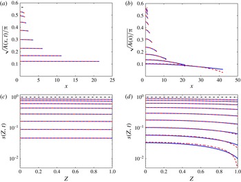
Comparison between the numerical solution (solid) and the small-inertia asymptotic solution (3.13) (dashed), with
 $L(t)=(1+t)^{{\it\alpha}}$
and
 $R=0.2$
for an initially cylindrical thread (dash-dot). The radius
 $\sqrt{A(x,t)/{\rm\pi}}$
is plotted against the physical coordinate
 $x$
for (a)
 ${\it\alpha}=0.4$
,
 ${\it\lambda}=200$
,
 $k=5,6,\ldots ,12$
, (b)
 ${\it\alpha}=0.8$
,
 ${\it\lambda}=100$
,
 $k=4,5,\ldots ,12$
. The extension of the thread doubles between subsequent curves (3.16). A better visualisation of these results is obtained by plotting cross-sectional area
 $s(Z,t)$
as a function of the Lagrangian variable
 $Z$
for the same parameters in (c,d). The asymptotic and numerical solutions are indistinguishable in (a,c), while the small-inertia solution can be seen to fail near the pulled end of the thread in (b,d).

Figure 2 compares the small-inertia solution (3.13) (dashed) with the numerical solution of (2.19) and (2.20) (solid) for
 $L(t)=(1+t)^{{\it\alpha}}$
for two different values of
 ${\it\alpha}>0$
. The numerical results were obtained using an implicit backward-time-centred-space (BTCS) finite difference scheme. The details are given in appendix A. In some sense, it is most physically natural to plot the the radius
 $\sqrt{A/{\rm\pi}}$
as a function of
 $x$
as done in figure 2(a,b). As is apparent, such plots have the problem that it becomes difficult to see the curves that represent early times when the thread becomes highly extended. We therefore plot the cross-sectional area
 $s(Z,t)$
as a function of the Lagrangian coordinate
 $Z$
; see (c,d). (Note that here, and throughout the remainder of the paper,
 $s(Z,t)\equiv A(x(Z,t),t)$
.) This has the advantage of fixing the domain between
 $Z=0$
and
 $Z=1$
at all times. The thread also becomes very thin during the stretching and we therefore use a logarithmic scale to plot
 $s(Z,t)$
. Curves are plotted at times
 $t$
when the thread extension is given by
 $$\begin{eqnarray}L(t)-1=\frac{2^{k}}{{\it\lambda}}\quad \text{for}~k=0,1,2,\ldots ,\end{eqnarray}$$
where
 ${\it\lambda}^{-1}$
is a chosen fraction of the initial length. Thus, the extension doubles between consecutive curves. The initial thread shape,
 $s_{0}(Z)=1$
is shown with a dash-dot line. In figure 2(a,c), we set
 ${\it\alpha}=0.4$
. As expected, the numerical solution and the small-inertia solution are indistinguishable from each other for all time. In figure 2(b,d), we set
 ${\it\alpha}=0.8$
. In this case the small-inertia solution fails near the pulled end of the thread at large time, as expected from our analysis. The final time in figure 2(a,c) is much greater than that in figure 2(b,d). The time corresponding to curve
 $k$
is
 $t_{k}=(1+2^{k}/{\it\lambda})^{1/{\it\alpha}}-1$
.
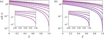
Comparison between the numerical solution (solid) and the small-inertia asymptotic solution (3.23) (dashed), with
 $L(t)=(1+t)^{{\it\alpha}}$
and
 $R=0.2$
for a thread that has its initial minimum at the pulled end (dash-dot). The cross-sectional area
 $s(Z,t)$
is plotted as a function of the Lagrangian variable
 $Z$
. The extension of the thread doubles between subsequent curves (3.16). Parameters are (a)
 ${\it\alpha}=0.8$
,
 ${\it\lambda}=100$
,
 $k=3,4,\ldots ,9$
, (b)
 ${\it\alpha}=2$
,
 ${\it\lambda}=100$
,
 $k=3,4,\ldots ,9$
. The asymptotic and numerical solutions are indistinguishable in (a), while the small inertia solution can be seen to fail near the pulled end of the thread in (b).

3.2 Case 2: thread with initial minimum at the pulled end
Next we consider a thread with initial shape
 $s_{0}(Z)=1+K(1-Z)$
. This thread shape has an initial minimum cross-sectional area at
 $Z=1$
and is shown for
 $K=1$
in figure 3 (dash-dot curve). Using (2.22) we find
 $$\begin{eqnarray}I=\displaystyle \frac{K}{\log (1+K)},\end{eqnarray}$$
and using (2.14) one can readily show that the initial condition in Eulerian coordinates is given by
 $A_{0}(x)=(1+K)^{1-x}$
, for
 $0\leqslant x\leqslant 1$
.
Substituting this initial thread shape into (2.19) yields
 $$\begin{eqnarray}RZ_{t}=Z_{xx}+\mathscr{K}Z_{x},\quad \text{with}~\mathscr{K}=\frac{K}{I}=\log (1+K),\end{eqnarray}$$
and the leading-order solution
 $Z_{0}$
satisfies
 $$\begin{eqnarray}Z_{0xx}+\mathscr{K}Z_{0x}=0,\quad \text{with}~Z_{0}(0,t)=0,~Z_{0}(L(t),t)=1,\end{eqnarray}$$
which has solution
 $$\begin{eqnarray}Z_{0}=\frac{1-\text{e}^{-\mathscr{K}x}}{1-\text{e}^{-\mathscr{K}L}}.\end{eqnarray}$$
The first-order correction satisfies
 $$\begin{eqnarray}\displaystyle Z_{1xx}+\mathscr{K}Z_{1x} & = & \displaystyle Z_{0t}\nonumber\\ \displaystyle & = & \displaystyle \displaystyle \frac{-\text{e}^{-\mathscr{K}L}\mathscr{K}\dot{L}(1-\text{e}^{-\mathscr{K}x})}{(1-\text{e}^{-\mathscr{K}L})^{2}}.\end{eqnarray}$$
Integrating twice with respect to
 $x$
and satisfying the boundary conditions
 $Z_{1}=0$
at
 $x=0$
and
 $x=L(t)$
we find
 $$\begin{eqnarray}Z_{1}=\displaystyle \frac{-\text{e}^{-\mathscr{K}L}\dot{L}}{(1-\text{e}^{-\mathscr{K}L})^{2}}\left(x(1+\text{e}^{-\mathscr{K}x})-L\frac{(1+\text{e}^{-\mathscr{K}L})}{(1-\text{e}^{-\mathscr{K}L})}(1-\text{e}^{-\mathscr{K}x})\right).\end{eqnarray}$$
Hence, to first order in
 $R$
 $$\begin{eqnarray}Z=\frac{1-\text{e}^{-\mathscr{K}x}}{1-\text{e}^{-\mathscr{K}L}}-\frac{R\text{e}^{-\mathscr{K}L}\dot{L}}{(1-\text{e}^{-\mathscr{K}L})^{2}}\left[x(1+\text{e}^{-\mathscr{K}x})-L\frac{(1+\text{e}^{-\mathscr{K}L})}{(1-\text{e}^{-\mathscr{K}L})}(1-\text{e}^{-\mathscr{K}x})\right].\end{eqnarray}$$
The cross-sectional area is readily calculated via
 $A=IZ_{x}$
.
Once again, we find the conditions under which the series for the cross-sectional area remains asymptotically valid by taking the ratio of the second and first terms:
 $$\begin{eqnarray}\displaystyle \displaystyle \frac{RA_{1}}{A_{0}}=\frac{RZ_{1x}}{Z_{0x}} & {\sim} & \displaystyle \frac{-R\text{e}^{-\mathscr{K}L}\dot{L}[1+\text{e}^{-\mathscr{K}x}-x\mathscr{K}\text{e}^{-\mathscr{K}x}-L(t)\mathscr{K}\text{e}^{-\mathscr{K}x}]}{\mathscr{K}\text{e}^{-\mathscr{K}x}}\nonumber\\ \displaystyle & {\sim} & \displaystyle -\frac{R}{\mathscr{K}}\text{e}^{-\mathscr{K}(L-x)}\dot{L}[1+\text{e}^{-\mathscr{K}x}(1-x\mathscr{K}-L(t)\mathscr{K})].\end{eqnarray}$$
We see that this expression is largest where
 $x=L(t)$
, and at this location
 $$\begin{eqnarray}\displaystyle \frac{RA_{1}}{A_{0}}\sim -\frac{R\dot{L}}{\mathscr{K}}.\end{eqnarray}$$
At early times,
 $$\begin{eqnarray}R\dot{L}\ll 1\end{eqnarray}$$
and the series is asymptotically valid. However, as for the cylindrical case, the validity at large times depends on the asymptotic behaviour of
 $L$
. If
 $L\sim t^{{\it\alpha}}$
as
 $t\rightarrow \infty$
, then
 $R\dot{L}/\mathscr{K}\sim Rt^{{\it\alpha}-1}/\mathscr{K}$
. This ratio gets smaller as
 $t$
increases for
 ${\it\alpha}<1$
and for
 ${\it\alpha}=1$
it will be a small constant of order
 $R$
. Thus, this small-inertia solution (3.23) will be valid for all time if
 ${\it\alpha}\leqslant 1$
. However, if
 ${\it\alpha}>1$
, the second term will, over time, dominate the first and the solution will no longer be asymptotically valid. Physically this is because inertia becomes important. We defer examination of this to § 4.
Figure 3 compares the small-inertia asymptotic solution (3.23) (dashed) with the numerical solution (solid). Once again, we plot the cross-sectional area (on a log scale) as a function of the Lagrangian variable so as to clearly show the change in the geometry of the thread as it becomes extremely long and thin. Curves are shown at times satisfying (3.16) for
 ${\it\lambda}=100$
,
 $k=0,1,\ldots ,9$
, and the dash-dot curve shows the initial thread shape.
Figure 3(a) shows the behaviour when
 ${\it\alpha}=0.8$
. The small-inertia and numerical solutions are almost indistinguishable, even when the extension is very large. In figure 3(b), we plot the behaviour when
 ${\it\alpha}=2$
. In this case, the small-inertia solution deviates from the numerical solution when the extension becomes large at long times. The failure of the small-inertia solution occurs at the pulled end of the thread. We note that, because of the different values of
 ${\it\alpha}$
, the final time in figure 3(a) is much greater than that in figure 3(b), although the final thread lengths are the same.
3.3 Case 3: thread with initial minimum away from the pulled end
The last case we consider is
 $s_{0}(Z)=1+KZ^{2}$
with
 $K>0$
. This represents an initial thread shape that has the minimum cross-sectional area at
 $Z=0$
. This initial shape is shown as a dash-dot line in figure 4. Using (2.22) and (2.14), we find that
 $$\begin{eqnarray}I=\frac{\sqrt{K}}{\tan ^{-1}(\sqrt{K})}.\end{eqnarray}$$
The corresponding initial thread shape in Eulerian coordinates is
 $A_{0}(x)=1+\tan ^{2}(x\tan ^{-1}(\sqrt{K}))$
, for
 $0\leqslant x\leqslant 1$
.
For this initial geometry, (2.19) reduces to
 $$\begin{eqnarray}RZ_{t}=Z_{xx}-2\mathscr{K}ZZ_{x},\quad \mathscr{K}=K/I.\end{eqnarray}$$
The leading-order solution
 $Z_{0}$
satisfies
 $$\begin{eqnarray}Z_{0xx}-2\mathscr{K}Z_{0}Z_{0x}=0,\quad \text{with}~Z_{0}(0,t)=0,~Z_{0}(L(t),t)=1.\end{eqnarray}$$
By integrating and making use of the boundary conditions, we find
 $$\begin{eqnarray}Z_{0}=f(t)\tan (\mathscr{K}f(t)x),\end{eqnarray}$$
where
 $f(t)$
satisfies the algebraic equation
 $$\begin{eqnarray}\frac{1}{f(t)}\tan ^{-1}\left(\frac{1}{f(t)}\right)=\mathscr{K}L(t).\end{eqnarray}$$
The
 $O(R)$
correction satisfies
 $$\begin{eqnarray}Z_{1xx}-2\mathscr{K}(Z_{0}Z_{1})_{x}=~Z_{0t}\quad \text{with}~Z(0,t)=0,~Z_{1}(L,t)=0.\end{eqnarray}$$
On substituting
 $Z_{0}$
, integrating twice with respect to
 $x$
and satisfying the boundary conditions, we find
 $Z_{1}$
. Hence, the solution for
 $Z$
to first order in
 $R$
is
 $$\begin{eqnarray}Z=f\tan (\mathscr{K}fx)+\frac{R{\dot{f}}}{2\mathscr{K}f}\left[-x+\frac{\mathscr{K}Lf^{2}}{\mathscr{K}L(f^{2}+1)+1}\left(x\sec ^{2}(\mathscr{K}fx)+\frac{\tan (\mathscr{K}fx)}{\mathscr{K}f}\right)\right],\end{eqnarray}$$
where the dot denotes differentiation with respect to
 $t$
.
Once again, we ensure the asymptotic validity of the series for the cross-sectional area by examining the ratio
 $$\begin{eqnarray}\displaystyle \frac{RA_{1}}{A_{0}}=\displaystyle \frac{RZ_{1x}}{Z_{0x}}=\displaystyle \frac{R{\dot{f}}}{2\mathscr{K}^{2}f^{3}}\left[-\cos ^{2}(\mathscr{K}fx)+\displaystyle \frac{\mathscr{K}Lf^{2}}{\mathscr{K}L(f^{2}+1)+1}(2-2\mathscr{K}fx\tan (\mathscr{K}fx))\right].\end{eqnarray}$$
Using (3.31) and the fact that
 $f$
becomes small and
 $\mathscr{K}L$
becomes large at large times, one can show that
 $RA_{1}/A_{0}$
is largest where
 $x=0$
. At this location
 $$\begin{eqnarray}\displaystyle \frac{RA_{1}}{A_{0}}\sim \displaystyle \frac{R{\dot{f}}}{f^{3}}.\end{eqnarray}$$
At early times,
 $$\begin{eqnarray}Rf^{-3}{\dot{f}}\ll 1\end{eqnarray}$$
and the series is asymptotically valid. However, at large times, the validity depends on the asymptotic behaviour of
 $L$
. From (3.31), we note that
 $f=O(1/(\mathscr{K}L))$
as
 $L\rightarrow \infty$
. If
 $L\sim t^{{\it\alpha}}$
as
 $t\rightarrow \infty$
, then
 $R{\dot{f}}/f^{3}=O(Rt^{2{\it\alpha}-1})$
. This quantity gets smaller for
 ${\it\alpha}<1/2$
and for
 ${\it\alpha}=1/2$
it will be a small constant. Thus, this small-inertia solution will be asymptotically valid for all time if
 ${\it\alpha}\leqslant 1/2$
. For larger values of
 ${\it\alpha}$
, the second term will eventually become larger than the first and so (3.33) loses validity. We consider
 ${\it\alpha}>1/2$
at large time in § 4.
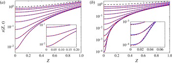
Figure 4 compares the numerical solution (solid) with the small-inertia solution (3.33) (dashed). As before, we plot the log of the cross-sectional area as a function of the Lagrangian coordinate to enable better comparison of the curves as the extension becomes large and the thread becomes thin. The extension doubles between successive curves and the initial thread shape is shown by a dash-dot curve.
Comparison between the numerical solution (solid) and the small-inertia asymptotic solution (3.33) (dashed), with
 $L(t)=(1+t)^{{\it\alpha}}$
and
 $R=0.2$
for a thread that has its initial minimum away from the pulled end (dash-dot). The cross-sectional area
 $s(Z,t)$
is plotted as a function of the Lagrangian variable
 $Z$
. The extension of the thread doubles between subsequent curves (3.16). Parameters are (a)
 ${\it\alpha}=0.4$
,
 ${\it\lambda}=200$
,
 $k=5,6,\ldots ,12$
, (b)
 ${\it\alpha}=0.8$
,
 ${\it\lambda}=10$
,
 $k=4,5,\ldots ,14$
. The asymptotic and numerical solutions are indistinguishable in (a), while the small inertia solution can be seen to fail near the centre (
 $Z=x=0$
) of the thread in (b).

Figure 4(a) shows the thread behaviour for
 ${\it\alpha}=0.4$
and figure 4(b) shows the behaviour for
 ${\it\alpha}=0.8$
. For
 ${\it\alpha}=0.4$
, the small-inertia solution is indistinguishable from the numerical solution for all times. In fact, closer examination of the curves shows that as time increases, the relative difference between the numerical and asymptotic solutions decreases. In contrast, for the case in which
 ${\it\alpha}=0.8$
, the asymptotic solution is seen to fail at large times where the relative difference between it and the numerical solution becomes significant. This failure occurs near
 $x=0$
, where the cross-sectional area is initially at a minimum. These results are fully consistent with the theory which states that inertia can only become important for values of
 ${\it\alpha}>1/2$
.
4 Solution at large time
In all three cases, we have seen that the small-inertia solutions fail at large times for
 ${\it\alpha}$
exceeding a critical value. We now obtain large-time solutions in the cases for which the small-inertia solution fails.
4.1 Case 1: initially cylindrical thread
In the case of an initially cylindrical thread, the critical value is
 ${\it\alpha}=1/2$
and we look for solutions of
 $$\begin{eqnarray}RZ_{t}=Z_{xx}\quad \text{with}~\left\{\begin{array}{@{}ll@{}}Z=x & \text{at}~t=0,0\leqslant x\leqslant 1\\ Z=0 & \text{at}~x=0\\ Z=1 & \text{at}~x=L(t),\end{array}\right.\end{eqnarray}$$
where
 $L(t)\sim t^{{\it\alpha}}$
at large times and
 ${\it\alpha}>1/2$
.
Using heat kernels, the fundamental solution that satisfies the boundary condition
 $Z=0$
at
 $x=0$
is (Carslaw & Jaeger Reference Carslaw and Jaeger1959)
 $$\begin{eqnarray}Z(x,t)=\int _{0}^{\infty }K({\it\xi},x,t;R){\it\phi}({\it\xi})\,\text{d}{\it\xi}\end{eqnarray}$$
where
 $$\begin{eqnarray}K({\it\xi},x,t;R)=\sqrt{\displaystyle \frac{R}{4{\rm\pi}t}}[\text{e}^{-R({\it\xi}-x)^{2}/4t}-\text{e}^{-R({\it\xi}+x)^{2}/4t}]\end{eqnarray}$$
and the function
 ${\it\phi}({\it\xi})$
must be chosen to satisfy the initial condition and the condition at the pulled end.
Taking the limit of (4.2) as
 $t\rightarrow 0$
, we see that the kernel becomes the sum of two delta functions,
 $$\begin{eqnarray}K({\it\xi},x,t;R)\rightarrow {\it\delta}({\it\xi}-x)+{\it\delta}({\it\xi}+x),\end{eqnarray}$$
and since
 $Z=x$
for
 $0\leqslant x\leqslant 1$
at
 $t=0$
, this allows us to determine that
 ${\it\phi}({\it\xi})={\it\xi}$
for
 $0\leqslant {\it\xi}\leqslant 1$
.
To find
 ${\it\phi}({\it\xi})$
for
 ${\it\xi}>1$
, we apply the boundary condition at the pulled end
 $x=L(t)$
, so that we require
 $$\begin{eqnarray}1=\int _{0}^{\infty }K({\it\xi},L,t;R){\it\phi}({\it\xi})\,\text{d}{\it\xi},\end{eqnarray}$$
which is a Fredholm integral equation of the first kind. It is more convenient to rewrite this equation in terms of
 $\widetilde{{\it\phi}}$
where
 ${\it\phi}=1+\widetilde{{\it\phi}}$
. Using the fact that
 $\int _{0}^{\infty }[\text{e}^{-({\it\xi}-a)^{2}}-\text{e}^{-({\it\xi}-a)^{2}}]\,\text{d}{\it\xi}=\sqrt{{\rm\pi}}\,\text{erf}(a)$
, and
 $\widetilde{{\it\phi}}={\it\xi}-1$
for
 $0<{\it\xi}<1$
, we obtain
 $$\begin{eqnarray}\int _{1}^{\infty }K({\it\xi},L,t;R)\widetilde{{\it\phi}}({\it\xi})\,\text{d}{\it\xi}=\text{erfc}\left(\sqrt{\frac{R}{4t}}L\right)-\int _{0}^{1}K({\it\xi},L,t;R)({\it\xi}-1)\,\text{d}{\it\xi},\end{eqnarray}$$
where
 $\text{erfc}(x)$
is the complementary error function.
In the following discussion, we will show that
 $\widetilde{{\it\phi}}({\it\xi})\rightarrow 0$
as
 ${\it\xi}\rightarrow \infty$
. We then use this, together with (4.2) to obtain an asymptotic solution for
 $Z(x,t)$
at large times.
At large times,
 $L(t)$
becomes large and the second exponential term in the kernel can be neglected as it represents a Gaussian centred at
 ${\it\xi}=-L(t)$
which is far from the area of interest,
 ${\it\xi}\in [1,\infty )$
. Thus, the kernel is approximately a Gaussian, centred at
 ${\it\xi}=L(t)$
with width
 $O(\sqrt{t/R})$
. Since
 $L\gg t^{1/2}$
, the kernel is such that at large
 $t$
, the contribution to the integral from values of
 ${\it\xi}=O(1)$
is small. Whilst the following argument can be couched in terms of operator theory, it is perhaps more straightforward to discuss it in terms of a discretised problem in matrix form. To discretise the integral on the left-hand side of (4.6), we rewrite it as a matrix,
 $\unicode[STIX]{x1D648}$
, multiplied by a column vector of unknowns,
 $\widetilde{\unicode[STIX]{x1D731}}$
. The right-hand side of the equation is a known column vector,
 $\boldsymbol{B}$
.
The matrix
 $\unicode[STIX]{x1D648}$
is constructed using the kernel,
 $K({\it\xi},L,t;R)$
. As discussed above, this kernel is approximately Gaussian, centred at
 $L(t)\gg t^{1/2}$
with a width which broadens like
 $t^{1/2}$
. As a result, if one chooses an appropriate discretisation for
 ${\it\xi}$
and
 $t$
, it can readily be seen that
 $\unicode[STIX]{x1D648}$
is dominated by the entries on its diagonal. Moreover, the matrix entries decay extremely rapidly as one moves away from the diagonal.
The vector
 $\boldsymbol{B}$
is constructed using the right-hand side of (4.6). After some straightforward calculation, one can see that the values of
 $\boldsymbol{B}$
are
 $O(1)$
at the top of the vector, but decay to zero in a Gaussian manner as one moves down the vector. As mentioned above,
 $\unicode[STIX]{x1D648}$
is dominated by the entries on its diagonal and has entries that decay rapidly as one moves away from the diagonal. As a consequence, the inverse matrix
 $\unicode[STIX]{x1D648}^{-1}$
also has the same form (Demko, Moss & Smith Reference Demko, Moss and Smith1984). As a result of these two properties,
 $\widetilde{\unicode[STIX]{x1D731}}$
will decay to zero as one moves down the vector. In terms of functions, this result corresponds to
 $\widetilde{{\it\phi}}({\it\xi})\rightarrow 0$
or
 ${\it\phi}({\it\xi})\rightarrow 1$
as
 ${\it\xi}\rightarrow \infty$
.
In order to evaluate
 $Z(x,t)$
, we now examine (4.2). For large times, the kernel broadens like
 $t^{1/2}$
, so that the contribution to the integral from
 ${\it\xi}=O(1)$
becomes less significant as
 $t\rightarrow \infty$
. This means that the integral can be approximated by setting
 ${\it\phi}=1$
, which gives the leading-order solution
 $$\begin{eqnarray}Z(x,t)=\text{erf}\left(\sqrt{\frac{R}{4t}}x\right).\end{eqnarray}$$
To calculate the cross-sectional area, we use
 $A=IZ_{x}$
to obtain
 $$\begin{eqnarray}A=\sqrt{\frac{R}{{\rm\pi}t}}\text{e}^{-Rx^{2}/4t}.\end{eqnarray}$$
Figure 5 compares the error function solution (4.7) (dashed) to the numerical solution (solid) for the initially cylindrical thread at large times, for
 ${\it\alpha}>1/2$
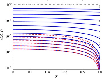
. As before, we plot the cross-sectional area on a log scale and as a function of the Lagrangian coordinate. The extension doubles between subsequent curves. The figure shows that at very large times when the thread is very thin, the error function solution is an extremely good approximation to the numerical solution. The error function solution has not been plotted at early times when the agreement is poor.
Comparison between the numerical solution (solid) and the large-time asymptotic solution (4.7) (dashed) with
 $L(t)\sim t^{{\it\alpha}}$
,
 ${\it\alpha}=0.8$
and
 $R=0.2$
. The cross-sectional area
 $s(Z,t)$
is plotted as a function of the Lagrangian variable
 $Z$
. Curves are plotted at times given by (3.16) with
 ${\it\lambda}=20$
. The numerical solution is shown for
 $k=4,5,\ldots ,16$
while the asymptotic solution is shown for
 $k=11,12,\ldots ,16$
. The initial condition is shown with a dash-dot line. As time increases, the asymptotic solution better approximates the numerical solution.

It is of interest to examine the form of the asymptotic correction to the solution. To do this, one must determine
 $\widetilde{{\it\phi}}$
from (4.6). The right-hand side of (4.6) contains two terms: a complementary error function and an integral involving the initial condition. As
 $t\rightarrow \infty$
,
 $$\begin{eqnarray}\text{erfc}\left(\sqrt{\frac{R}{4t}}L\right)\sim \sqrt{\frac{4t}{{\rm\pi}R}}\displaystyle \frac{\text{e}^{-RL^{2}/4t}}{L},\end{eqnarray}$$
and
 $$\begin{eqnarray}\int _{0}^{1}K({\it\xi},L,t;R)({\it\xi}-1)\,\text{d}{\it\xi}\sim -\displaystyle \frac{2t^{3/2}}{\sqrt{{\rm\pi}}R^{3/2}}\frac{1}{L^{2}}\text{e}^{-R(L-1)^{2}/4t}.\end{eqnarray}$$
The ratio of these two terms has the following asymptotic form
 $$\begin{eqnarray}\frac{\displaystyle \int _{0}^{1}K({\it\xi},L,t;R)({\it\xi}-1)\,\text{d}{\it\xi}}{\text{erfc}\left(\sqrt{\displaystyle \frac{R}{4t}}L\right)}\sim \frac{t}{RL}\text{e}^{RL/2t}.\end{eqnarray}$$
In the case
 $L\gg t$
(
 ${\it\alpha}>1$
), the ratio becomes exponentially large as
 $t\rightarrow \infty$
. For
 $L\ll t$
(
 ${\it\alpha}<1$
), the ratio grows like
 $t^{1-{\it\alpha}}/R$
as
 $t\rightarrow \infty$
. Finally, in the case
 $L\sim t$
(
 ${\it\alpha}=1$
), the ratio tends to a large constant of size
 $O(1/R)$
. In all three cases, at large times, the integral involving the initial condition is larger than the complementary error function and so the right-hand side of (4.6) will eventually be dominated by the integral involving the initial conditions. Thus, even for large
 ${\it\xi}$
, the asymptotic correction
 $\widetilde{{\it\phi}}$
will also depend on the initial conditions, and as a result, one cannot find an asymptotic correction that is only determined by the local behaviour near the pulled end. For diffusive problems of this type, the effects of the initial condition decay exponentially quickly as time goes to infinity. However, for this problem, the leading-order asymptotic correction is also exponentially small and so the initial condition remains significant indefinitely.
4.2 Case 2: thread with initial minimum at the pulled end
Next we consider a thread in which the initial minimum occurs at the pulled end, i.e.
 $s_{0}(Z)=1+K(1-Z)$
, in the case in which inertia eventually becomes important, i.e.
 $L\sim t^{{\it\alpha}}$
for
 ${\it\alpha}>1$
. Figure 3(b) demonstrates that for values of
 ${\it\alpha}>1$
, the small-inertia solution fails near the pulled end of the thread. In the following, we show that the small-inertia solution is valid in the main part of the thread, even at large times.
It proves to be convenient to rewrite the governing equation (2.19) in terms of coordinates
 $(Z,{\it\tau})$
, rather than
 $(x,t)$
, where
 ${\it\tau}=t$
and the Lagrangian variable
 $Z$
is an independent variable. In addition, fluid elements travel with the fluid velocity so that
 $u=x_{{\it\tau}}$
. Multiplying the governing equation (2.19) by
 $I$
, using (2.14) and (2.16), we obtain
 $$\begin{eqnarray}IRu=(s_{0}-s)_{Z}.\end{eqnarray}$$
Partially differentiating with respect to
 $Z$
and using
 $u=x_{{\it\tau}}$
and (2.14), we obtain
 $$\begin{eqnarray}I^{2}R\left(\displaystyle \frac{1}{s}\right)_{{\it\tau}}=(s_{0}-s)_{ZZ}.\end{eqnarray}$$
A more detailed derivation of this equation can be found in Wylie et al. (Reference Wylie, Huang and Miura2011).
At large times and in regions away from the pulled end, the right-hand side of (4.13) is
 $O(1)$
. Since
 $s$
is also
 $O(1)$
here, and
 $R$
is small, the left-hand side is small. From this, it follows that in regions away from the pulled end,
 $(s_{0}-s)_{ZZ}=0$
approximately describes the evolution of the thread. This precisely corresponds to the small-inertia problem (3.18) of § 3.2. We therefore conclude that the small-inertia solution is valid for a large portion of the thread, even at large times and when
 ${\it\alpha}>1$
. This can be confirmed by examining figure 3.
In contrast, at large times and near the end of the thread,
 $s$
becomes small so that the left-hand side of (4.13) becomes significant. In fact, inertia will be important in regions near the end of the thread where
 $s=O(R)$
. In this case, we must solve (4.13) in its entirety, together with the appropriate initial and boundary conditions.
To examine how the thread shape changes near the pulled end, we look for a large-time asymptotic solution there. Using the transformation
 $p(x,t)=\text{e}^{\mathscr{K}x/2+\mathscr{K}^{2}t/4R}Z(x,t)$
, the governing equation (3.18) can be rewritten as the heat equation, however the initial and boundary conditions become more complicated. Using the same technique as that presented in § 4.1, we find that, in the original coordinates, the leading-order term at large times near the end of the thread is
 $Z\sim 1$
. As in the case of the cylinder, we find that the dominant contribution to the first correction term involves the initial condition. Since the influence of the initial condition does not become negligible near the end of the thread as
 $t\rightarrow \infty$
, it is not possible to find an asymptotic correction that is determined only by the local behaviour at the end.
Therefore, in summary, the majority of the stretching occurs in fluid elements that originated near the pulled end. For these fluid elements, inertia is important. However, for fluid elements that originated in the main portion of the thread, inertia is always negligible so that the small-inertia solution is valid, even at large times.
4.3 Case 3: thread with initial minimum away from the pulled end
For the case
 $s_{0}(Z)=1+KZ^{2}$
, the governing equation is
 $$\begin{eqnarray}RZ_{t}=Z_{xx}-2\mathscr{K}ZZ_{x},\end{eqnarray}$$
where
 $\mathscr{K}$
is defined in § 3.3. The boundary conditions are
 $Z(0,t)=0$
and
 $Z(L(t),t)=1$
, with
 $L(t)\sim t^{{\it\alpha}}$
at large times. The small-inertia solution given by (3.30) and (3.33), whilst valid for all times when
 ${\it\alpha}\leqslant 1/2$
, was shown to fail at large times when
 ${\it\alpha}>1/2$
. We therefore now consider the case
 $L(t)\gg t^{1/2}$
.
From (3.30) and (3.33), we anticipate that
 $s(Z,t)$
will become small in the middle of the thread. In this case, the natural scalings of (4.14) suggest that we make the transformation
 $$\begin{eqnarray}Z=\frac{R^{1/2}}{\mathscr{K}t^{1/2}}G({\it\eta},{\it\tau}),\end{eqnarray}$$
where
 $$\begin{eqnarray}{\it\eta}=\frac{R^{1/2}x}{2t^{1/2}}\quad \text{and}\quad {\it\tau}=t.\end{eqnarray}$$
Writing (4.14) in terms of these new variables yields
 $$\begin{eqnarray}G_{{\it\eta}{\it\eta}}+2({\it\eta}G)_{{\it\eta}}-2(G^{2})_{{\it\eta}}=4{\it\tau}G_{{\it\tau}},\end{eqnarray}$$
with boundary conditions
 $$\begin{eqnarray}G(0)=0\quad \text{and}\quad G\left(\frac{R^{1/2}L({\it\tau})}{2{\it\tau}^{1/2}}\right)=\frac{\mathscr{K}{\it\tau}^{1/2}}{R^{1/2}}.\end{eqnarray}$$
We proceed by neglecting the
 ${\it\tau}G_{{\it\tau}}$
term in (4.17). A priori it is unclear that this term is negligible, but after obtaining the solution, we will verify that it is indeed the case. Under this assumption, (4.17) becomes an ordinary differential equation in
 ${\it\eta}$
with
 ${\it\tau}$
as a parameter. After integrating with respect to
 ${\it\eta}$
, we obtain
 $$\begin{eqnarray}G_{{\it\eta}}+2{\it\eta}G-2G^{2}=2c({\it\tau})+{\textstyle \frac{1}{2}},\end{eqnarray}$$
where
 $c({\it\tau})$
is an arbitrary function of
 ${\it\tau}$
. The solution to (4.19) can be obtained in terms of Whittaker functions and is given by
 $$\begin{eqnarray}G=\frac{4c+1}{4{\it\eta}}+\frac{4D({\it\tau})W_{c+1,1/4}({\it\eta}^{2})-(4c+3)M_{c+1,1/4}({\it\eta}^{2})}{4{\it\eta}[D({\it\tau})W_{c,1/4}({\it\eta}^{2})+M_{c,1/4}({\it\eta}^{2})]},\end{eqnarray}$$
where
 $D({\it\tau})$
is an arbitrary function of
 ${\it\tau}$
. Applying the boundary condition
 $G(0)=0$
and making use of the small
 ${\it\eta}$
asymptotics for the Whittaker function, one obtains
 $$\begin{eqnarray}D({\it\tau})=\frac{1}{2\sqrt{{\rm\pi}}}{\it\Gamma}\left(\frac{1}{4}-c({\it\tau})\right),\end{eqnarray}$$
where
 ${\it\Gamma}$
is the gamma function. Substituting this back into (4.20), we obtain
 $$\begin{eqnarray}G=\frac{4c+1}{4{\it\eta}}+\frac{2{\it\Gamma}({\textstyle \frac{1}{4}}-c)W_{c+1,1/4}({\it\eta}^{2})-\sqrt{{\rm\pi}}(4c+3)M_{c+1,1/4}({\it\eta}^{2})}{2{\it\eta}[{\it\Gamma}({\textstyle \frac{1}{4}}-c)W_{c,1/4}({\it\eta}^{2})+2\sqrt{{\rm\pi}}M_{c,1/4}({\it\eta}^{2})]}.\end{eqnarray}$$
This has asymptotic form
 $$\begin{eqnarray}G\sim {\textstyle \frac{1}{2}}(4c+1){\it\eta}+O({\it\eta}^{2})\quad \text{as}~{\it\eta}\rightarrow 0.\end{eqnarray}$$
Since, we require that
 $G>0$
, we must restrict our attention to
 $c>-1/4$
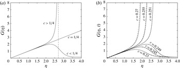
. In figure 6(a), we illustrate that the function
 $G$
must exhibit one of three different types of behaviour for different values of
 $c$
. For
 $c<1/4$
,
 $G$
increases to a maximum value before eventually decaying to zero. For
 $c>1/4$
,
 $G$
has a singularity at a finite value of
 ${\it\eta}={\it\eta}_{\ast }$
and is a monotonic increasing function for
 $0<{\it\eta}<{\it\eta}_{\ast }$
. For
 $c=1/4$
, it is easy to check that the solution is given by the straight line
 $G={\it\eta}$
. The solution
 $G={\it\eta}$
separates the two solutions types for
 $c>1/4$
and
 $c<1/4$
. As
 $c\rightarrow 1/4^{+}$
, the value of
 ${\it\eta}_{\ast }\rightarrow \infty$
, whereas as
 $c\rightarrow 1/4^{-}$
, the location of the maximum tends to infinity. In both cases, for any fixed value of
 ${\it\eta}$
,
 $G\rightarrow {\it\eta}$
as
 $c\rightarrow 1/4$
.


We need to apply a boundary condition at
 ${\it\eta}=R^{1/2}L({\it\tau})/(2{\it\tau}^{1/2})$
. Since we are considering the case
 $L({\it\tau})\gg {\it\tau}^{1/2}$
, this value will become large in the long-time limit. In the case
 $c>1/4$
, we therefore require that the singularity at
 ${\it\eta}_{\ast }({\it\tau})$
is not in the domain
 $0\leqslant {\it\eta}\leqslant R^{1/2}L({\it\tau})/(2{\it\tau}^{1/2})$
. This implies that
 ${\it\eta}_{\ast }({\it\tau})$
must become large as
 ${\it\tau}\rightarrow \infty$
. On the other hand, in the case
 $c<1/4$
, we require that the location of the maximum is also not in the domain. This is because
 $G$
must be a monotonically increasing function of
 ${\it\eta}$
since
 $Z$
is, by definition, a monotonically increasing function of
 $x$
. These conditions can only be true if
 $c({\it\tau})\rightarrow 1/4$
as
 ${\it\tau}\rightarrow \infty$
. We therefore focus our attention on the
 $c({\it\tau})\rightarrow 1/4$
limit.
In the case
 $c({\it\tau})\rightarrow 1/4^{+}$
, we can obtain the location of the singularity
 ${\it\eta}_{\ast }$
by finding the zero of the denominator of the second fraction in (4.22), i.e. by solving
 $$\begin{eqnarray}{\it\Gamma}({\textstyle \frac{1}{4}}-c)W_{c,1/4}({\it\eta}^{2})+2\sqrt{{\rm\pi}}M_{c,1/4}({\it\eta}^{2})=0.\end{eqnarray}$$
Taking the limit as
 $c\rightarrow 1/4$
and using the large
 ${\it\eta}$
asymptotics of the Whittaker functions, we obtain
 $$\begin{eqnarray}c-\frac{1}{4}=\frac{{\it\eta}_{\ast }\text{e}^{-{\it\eta}_{\ast }^{2}}}{\sqrt{{\rm\pi}}}.\end{eqnarray}$$
We now obtain an approximation for (4.22), by taking the limit as
 $c({\it\tau})\rightarrow 1/4$
and noting that the expression should be valid for values of
 ${\it\eta}$
close to
 ${\it\eta}_{\ast }$
, that is
 $$\begin{eqnarray}G\sim \frac{1}{2{\it\eta}}+\frac{W_{5/4,1/4}({\it\eta}^{2})}{{\it\eta}[W_{1/4,1/4}({\it\eta}^{2})-2\sqrt{{\rm\pi}}(c-{\textstyle \frac{1}{4}})M_{1/4,1/4}({\it\eta}^{2})]}.\end{eqnarray}$$
In the above expression, we have retained the term
 $(c-1/4)M_{1/4,1/4}({\it\eta}^{2})$
, even though it is
 $O(c-1/4)$
smaller than the term
 $W_{5/4,1/4}({\it\eta}^{2})$
for
 ${\it\eta}=O(1)$
. This is because near
 ${\it\eta}={\it\eta}_{\ast }$
, the two terms are of similar order and it is the cancelation between these two terms that gives the singularity in (4.22). The Whittaker functions in (4.26) can be expressed in terms of simple functions to give
 $$\begin{eqnarray}G\sim \frac{1}{2{\it\eta}}+\frac{2{\it\eta}^{2}-1}{2{\it\eta}[1-{\rm\pi}(c-{\textstyle \frac{1}{4}})\text{erfi}({\it\eta})]},\end{eqnarray}$$
where
 $\text{erfi}(x)$
is the imaginary error function. We note that (4.27) is also valid for
 $c\rightarrow 1/4^{-}$
. The comparison between the asymptotic approximation (4.27) and (4.22) for
 ${\it\eta}$
near to
 $1/4$
is shown in figure 6(b). The asymptotic approximation shows good agreement even for relatively moderate values of
 ${\it\eta}_{\ast }$
.
In order to determine the value of
 $c({\it\tau})$
or equivalently
 ${\it\eta}_{\ast }({\it\tau})$
, we need to satisfy the boundary condition (4.18b
). To satisfy this condition, we require that
 $G\gg {\it\eta}$
, or
 $$\begin{eqnarray}\displaystyle \frac{\mathscr{K}t^{1/2}}{R^{1/2}}\gg \frac{LR^{1/2}}{2t^{1/2}}\end{eqnarray}$$
so that
 $L\ll t/R$
. Thus, we now assume that
 ${\it\alpha}\leqslant 1$
(so that
 $t^{1/2}\ll L\ll t$
) and return to the case where
 ${\it\alpha}>1$
later. The only solutions with
 $G>{\it\eta}$
are those with
 $c({\it\tau})>1/4$
which have a singularity at
 ${\it\eta}_{\ast }$
. Since
 $G/{\it\eta}\gg 1$
at
 ${\it\eta}=LR^{1/2}/(2{\it\tau}^{1/2})$
, we must choose the location of the singularity only slightly larger than
 ${\it\eta}=LR^{1/2}/(2{\it\tau}^{1/2})$
. To asymptotically satisfy the boundary condition, we first determine the asymptotics of (4.27) near
 ${\it\eta}={\it\eta}_{\ast }$
. Using (4.25) to eliminate
 $c$
from (4.27), expanding near
 ${\it\eta}={\it\eta}_{\ast }$
and assuming that
 ${\it\eta}_{\ast }$
is large, we obtain
 $$\begin{eqnarray}G\sim \frac{-1}{2({\it\eta}-{\it\eta}_{\ast })}\quad \text{for}~{\it\eta}\rightarrow {\it\eta}_{\ast }~\text{and}~{\it\eta}_{\ast }\gg 1.\end{eqnarray}$$
Applying (4.18b
) to (4.29), we obtain an expression for
 ${\it\eta}_{\ast }$
,
 $$\begin{eqnarray}{\it\eta}_{\ast }=\frac{R^{1/2}}{2t^{1/2}}(L({\it\tau})+\mathscr{K}^{-1})\quad \text{for}~{\it\eta}_{\ast }\gg 1.\end{eqnarray}$$
Using (4.25) and (4.27), we therefore obtain
 $$\begin{eqnarray}G\sim \frac{1}{2{\it\eta}}+\frac{2{\it\eta}^{2}-1}{2{\it\eta}[1-\sqrt{{\rm\pi}}{\it\eta}_{\ast }e^{-{\it\eta}_{\ast }^{2}}\,\text{erfi}({\it\eta})]},\end{eqnarray}$$
with
 ${\it\eta}_{\ast }$
given by (4.30). This represents the uniformly valid solution to the problem for case 3 with
 $L(t)\ll t/R$
.
We now need to check that the
 ${\it\tau}G_{{\it\tau}}$
term that we neglected in (4.17) is indeed negligible in comparison to the other terms in the equation. For
 ${\it\eta}=O(1)$
, this is clearly true since
 $G({\it\eta})\sim {\it\eta}$
. However, near
 ${\it\eta}={\it\eta}_{\ast }$
, the situation is more complicated. Using, the asymptotic form (4.29), we obtain
 $$\begin{eqnarray}{\it\tau}G_{{\it\tau}}\sim \frac{1}{2({\it\eta}-{\it\eta}_{\ast })^{2}}{\it\tau}\frac{\text{d}{\it\eta}_{\ast }}{\text{d}{\it\tau}}.\end{eqnarray}$$
Since
 ${\it\tau}^{1/2}\ll L({\it\tau})\ll {\it\tau}/R$
, we have
 ${\it\tau}\,\text{d}{\it\eta}_{\ast }/\text{d}{\it\tau}=O({\it\eta}_{\ast })$
and so
 $$\begin{eqnarray}{\it\tau}G_{{\it\tau}}=O\left(\frac{{\it\eta}_{\ast }}{({\it\eta}-{\it\eta}_{\ast })^{2}}\right).\end{eqnarray}$$
On the other hand, the term
 $(G^{2})_{{\it\eta}}=O(({\it\eta}-{\it\eta}_{\ast })^{-3})$
and therefore
 $$\begin{eqnarray}\frac{(G^{2})_{{\it\eta}}}{{\it\tau}G_{{\it\tau}}}=O\left(\frac{1}{{\it\eta}_{\ast }({\it\eta}-{\it\eta}_{\ast })}\right).\end{eqnarray}$$
Using (4.29) near
 ${\it\eta}=R^{1/2}L({\it\tau})/(2{\it\tau}^{1/2})$
to obtain the scaling for
 $({\it\eta}-{\it\eta}_{\ast })$
and (4.30) to obtain the scaling for
 ${\it\eta}_{\ast }$
, we have
 $$\begin{eqnarray}\frac{(G^{2})_{{\it\eta}}}{{\it\tau}G_{{\it\tau}}}=O\left(\frac{t}{\mathscr{K}RL}\right)\gg 1,\end{eqnarray}$$
since
 $L\ll t/R$
. Hence, we conclude that the term
 ${\it\tau}G_{{\it\tau}}$
is negligible.
We now analyse the solution and show that the majority of the stretching occurs for material that was initially located near the initial minimum. In (4.17), the
 $G_{{\it\eta}{\it\eta}}$
and
 $(G^{2})_{{\it\eta}}$
terms correspond to the
 $Z_{xx}$
and
 $ZZ_{x}$
terms in (4.14), that represent the viscous forces, whereas the
 $({\it\eta}G)_{{\it\eta}}$
term corresponds to the
 $RZ_{t}$
term that represents inertial forces. For
 ${\it\eta}\ll {\it\eta}_{\ast }$
,
 $G$
is well approximated by
 $G\sim {\it\eta}$
. In this case, the main balance is between the
 $(G^{2})_{{\it\eta}}$
and
 $({\it\eta}G)_{{\it\eta}}$
terms indicating that the main balance is between viscous and inertial forces. However, close to
 ${\it\eta}={\it\eta}_{\ast }$
, the solution is well approximated by
 $G\sim ({\it\eta}_{\ast }-{\it\eta})^{-1}/2$
and the main balance is between the
 $(G^{2})_{{\it\eta}}$
and the
 $G_{{\it\eta}{\it\eta}}$
terms. In this case, the inertial term
 $({\it\eta}G)_{{\it\eta}}$
is negligible. Hence, inertial terms are only significant when
 $G\sim {\it\eta}$
, which, using (4.15), corresponds to
 $Z=O(RL/t)\ll 1$
. This implies that inertia only ever becomes important for the material that was initially located near the local minimum. This material becomes stretched into a long thin thread that occupies the vast majority of the length. In this region
 $G\sim {\it\eta}$
, which corresponds to
 $Z\sim xR/(2\mathscr{K}t)$
. Since
 $A=IZ_{x}$
, we see that this region corresponds to a thin thread whose cross-section is
 $O(R)$
. Moreover, in this region, the cross-section is uniform in space, but decreases inversely with time. On the other hand, near the singularity,
 $G\sim ({\it\eta}_{\ast }-{\it\eta})^{-1}/2$
, which corresponds to
 $Z\sim [1-\mathscr{K}(x-L)]^{-1}$
. This shows that the fluid near the pulled end eventually experiences negligible thinning and is just advected along with the pulled boundary at
 $x=L(t)$
.
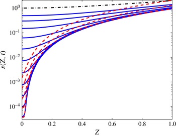
In figure 7 we compare the large-time solution given by (4.15), (4.27), for the case where
 $1/2<{\it\alpha}<1$
, with the numerical solution. Once again, we plot the solutions on a log scale and as a function of the Lagrangian coordinate. The agreement becomes better as time becomes larger and the thread becomes thinner, indicating the validity of the long-time solution. The long-time solution has not been plotted at early times when the agreement is poor. We note that, at later times, the region close to
 $Z=0$
represents an extremely long and thin filament that forms the vast majority of the length of the thread. As time increases, this filament becomes progressively longer and thinner while the remaining fluid experiences negligible thinning as we commented above.
Comparison between the numerical solution (solid) and the large-time solution given by (4.15) and (4.27) (dashed) with
 $L(t)\sim t^{{\it\alpha}}$
and
 $R=0.2$
for a thread that has its initial minimum away from the pulled end (dash-dot). The cross-sectional area
 $s(Z,t)$
is plotted as a function of the Lagrangian variable
 $Z$
. The extension of the thread doubles between successive curves (3.16). Here,
 ${\it\alpha}=0.8$
,
 ${\it\lambda}=40$
. The numerical solution is shown for
 $k=5,6,\ldots ,15$
, while the asymptotic solution is shown for
 $k=11,12,\ldots ,15$
. Agreement between the curves becomes better as time becomes larger and the thread becomes thinner.

Finally, we discuss the behaviour of this type of thread in the case where
 ${\it\alpha}>1$
. In this case, one can readily see that the expression (4.27), that corresponds to a solution in which the majority of the extension is concentrated in those fluid elements that were originally located near the initial minimum, cannot satisfy the boundary condition at
 $X=L(t)$
at large times.
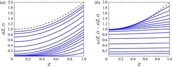
In figure 8(a), we plot results of a numerical simulation for
 ${\it\alpha}=2$
. At early times, the solution is well approximated by the small-inertia solution (3.33), but the approximation breaks down when
 $s$
becomes small (see figure 4
b). Beyond this time, the region in
 $Z$
in which the thread becomes thin expands as time progresses. This is in direct contrast to the case of
 $1/2<{\it\alpha}\leqslant 1$
, in which the thread only becomes thin in the vicinity of
 $Z=0$
. Thus, in the case
 ${\it\alpha}>1$
, the pulling rate is sufficiently fast that the extension cannot remain localised to fluid elements near the initial minimum.
Thinning of a thread with the initial minimum away from the pulled end for
 $R=0.2$
,
 ${\it\alpha}=2$
. The extension doubles between successive curves (3.16). We have used
 ${\it\lambda}=100$
. The solutions are shown for
 $k=3,4,\ldots ,16$
. (a) Cross-sectional area
 $s(Z,t)$
is plotted as a function of the Lagrangian variable
 $Z$
. (b) Departure from the cross-sectional area,
 $s_{0}(Z)-s(Z,t)$
.

Wylie et al. (Reference Wylie, Huang and Miura2011) showed that this type of behaviour must occur for threads pulled with a fixed force. They divided the
 $Z$
-space into two parts: an ‘outer region’ in which
 $s=O(1)$
and a ‘necking region’ in which
 $s$
is small. They considered the quantity
 $s_{0}-s$
which corresponds to the deviation from the initial shape and showed that, in the necking region,
 $s_{0}-s$
is small, whereas in the outer region,
 $s_{0}-s$
must be a linear function of
 $Z$
. They further showed that the two types of solutions must be patched together at a location at which
 $s_{0}-s$
and its derivative are continuous. Since the largest value that
 $s_{0}-s$
can attain is
 $s_{0}$
, the leading-order problem can be thought of as a purely geometrical obstacle problem with an elastic string whose end moves with time. The necking regions correspond to the regions in which the string is in contact with the object, whereas the outer regions correspond to the regions in which the string is not in contact with the object. In figure 8(b), we replot the data in figure 8(a) for the variable
 $s_{0}-s$
. The curve, which is initially an approximately horizontal line can clearly be seen to wrap around the obstacle. Using asymptotic methods, Wylie et al. (Reference Wylie, Huang and Miura2011) were able to obtain an explicit solution for the necking region that allowed them to compute the total extension. A similar approach can be used for the current problem, but since the methodology has been developed in detail in their paper, we will not repeat the details here.
5 Final remarks
In this paper, we have considered a symmetric thin viscous thread that is pulled from each end with a prescribed speed. Initial examination of the problem revealed two generic cases – the case where the initial minimum cross-sectional area is at the pulled ends and the case where the initial minimum is away from the ends of the thread. An example of each of these two different cases was analysed. In addition, we also analysed the simpler case of an initially cylindrical thread which has a different type of behaviour to the generic cases. For each case, we have found a solution which is valid when inertia is small.
Assuming that the length of the thread has asymptotic form
 $L(t)\sim t^{{\it\alpha}}$
, we analysed the large-time asymptotic behaviour of these solutions. We have shown that there is a critical value of
 ${\it\alpha}$
below which inertia never becomes important so that the small-inertia solutions are valid, even at large times when the thread is very long and thin. For values of
 ${\it\alpha}$
above critical, inertia becomes important at large times and the small-inertia solutions are no longer valid. Moreover, the critical value of
 ${\it\alpha}$
is different for the two generic cases.
For values of
 ${\it\alpha}$
which are larger than the critical value, each type of thread exhibits radically different behaviour. In the case of an initially cylindrical thread, the critical value is
 ${\it\alpha}=1/2$
. For
 ${\it\alpha}>1/2$
, we have found an asymptotic solution that is valid for large times. We have shown that, the asymptotic correction to the solution depends on the initial condition. Therefore it is not possible to find an asymptotic correction that is determined only by the local behaviour near the pulled end.
In the case of a thread that has its initial minimum at the pulled end, the critical value is
 ${\it\alpha}=1$
. For
 ${\it\alpha}>1$
, we have shown that the small-inertia solution is valid even at large times, except in a region very close to the pulled end. Near the pulled end, as was the case for the cylindrical thread, the leading-order solution depends on the initial condition. Therefore, one cannot find an asymptotic solution that depends on only the local behaviour near the pulled end.
In the case of a thread for which the initial minimum cross-sectional area is located away from the end of the thread, the critical value is
 ${\it\alpha}=1/2$
. For
 ${\it\alpha}>1/2$
, there are two different regimes. For
 $1/2<{\it\alpha}\leqslant 1$
, we have found an asymptotic solution in which the majority of the extension is concentrated in those fluid elements that were originally located near the initial minimum. This solution is valid at large times and can be expressed in terms of Whittaker functions. For
 ${\it\alpha}>1$
, the problem can be recast as an obstacle problem and the solution can be obtained using the theory developed in Wylie et al. (Reference Wylie, Huang and Miura2011). In this case, the extension does not remain localised as occurred in the
 $1/2<{\it\alpha}\leqslant 1$
case.
While we have used the asymptotic form
 $L(t)\sim t^{{\it\alpha}}$
to delineate the various cases, the analysis can be readily extended to other functional forms for
 $L(t)$
. For example, in the rheologically important case of exponential stretching, in which
 $L\sim \text{e}^{\hat{{\it\alpha}}t}$
, the conditions (3.15), (3.26) and (3.36) will always be violated for sufficiently large time regardless of the value of
 $\hat{{\it\alpha}}$
. That is, inertia will always become important.
We now discuss the issue of the boundary condition at the pulled end. When solving the full Navier–Stokes equations, one typically requires two boundary conditions at the pulled end. Typically, one would apply zero velocity through the boundary and no-slip. The long-wavelength equations are a singular perturbation of the Navier–Stokes equations and one must drop one of the boundary conditions. In the context of pulled threads, it is most natural to drop the no-slip condition. Therefore, the solution of the long-wavelength equations must be supplemented by a boundary layer of width
 ${\it\epsilon}$
in which the velocity depends on the radial coordinate. Hence, solutions of the long-wavelength equations will only be strictly valid for
 $L(t)-x\gg {\it\epsilon}$
.
Finally, we address the issue of surface tension. Wylie et al. (Reference Wylie, Huang and Miura2011) showed that for a thread extended by a fixed force, the surface tension always remains negligible compared to the viscous stress and the inertial terms. Clearly, as the thread thins, the resistance to stretching decreases. Thus, they were able to show that a fixed force gives an asymptotically large speed of the end points. However, in the current problem, the pulling speed is fixed and one can readily show that, as cross-sectional area decreases, the force required to stretch the thread must also decrease. It therefore seems natural that the extensional force will eventually become small enough that surface tension will become important. Thus, even if the surface tension force was initially negligible, it may ultimately become dominant and cause the thread to pinch.
In order to properly include surface tension effects in this problem, the surface tension term must be retained in (2.11). After rewriting the equations in terms of the Lagrangian variable,
 $Z(x,t)$
, (2.18) will contain a term involving surface tension. Integrating with respect to material time is problematic since the surface tension term must be time integrated whilst holding the Lagrangian coordinate,
 $Z(x,t)$
, constant (see also Bradshaw-Hajek et al.
Reference Bradshaw-Hajek, Stokes and Tuck2007). We thus leave the detailed consideration of surface tension to a future paper.
However, it is possible to use asymptotic estimates to determine criteria for the surface tension term to remain negligible for each of the solutions we have obtained. If we retain the surface tension term in (2.17), we obtain
 $$\begin{eqnarray}R\frac{\text{D}}{\text{D}t}\left(\frac{Z_{t}}{Z_{x}}\right)=\frac{1}{Z_{x}}\frac{\partial }{\partial x}\left(\frac{\text{D}}{\text{D}t}(Z_{x})+{\it\Gamma}I^{-1/2}Z_{x}^{1/2}\right).\end{eqnarray}$$
The surface tension force will remain negligible if it is small compared with the viscous force. That is,
 $$\begin{eqnarray}\frac{\text{D}}{\text{D}t}(Z_{x})\gg {\it\Gamma}Z_{x}^{1/2}.\end{eqnarray}$$
We begin by considering the solutions we obtained when inertial effects were small for each of the three different initial shapes. For case 1 (the initially cylindrical thread), substituting the leading-order term of (3.13) into (5.2), we find that surface tension is negligible while
 ${\it\Gamma}\ll \dot{L}L^{-3/2}$
. Therefore, the time,
 $t_{ST}$
, at which surface tension first becomes important is given by
 $t_{ST}\sim {\it\Gamma}^{-2/({\it\alpha}+2)}$
. We recall that inertial effects never become significant in (3.13) for
 ${\it\alpha}\leqslant 1/2$
, but become important at time
 $t_{INERT}\sim R^{-1/(2{\it\alpha}-1)}$
for
 ${\it\alpha}>1/2$
. Therefore, for
 ${\it\alpha}>1/2$
, in order for inertia to become important before surface tension, we require that
 $t_{INERT}\ll t_{ST}$
or, equivalently,
 $R\gg {\it\Gamma}^{2(2{\it\alpha}-1)/({\it\alpha}+2)}$
. The other two cases may be examined similarly. The results for all three cases are summarised in table 1.
The times
 $t_{ST}$
and
 $t_{INERT}$
at which surface tension and inertia become important, respectively, for each of the three thread cases considered in this paper with
 $L(t)\sim t^{{\it\alpha}}$
. The last column shows the condition for inertia to become important before surface tension.

Acknowledgements
The authors acknowledge financial support from the Research Grants Council of the Hong Kong Special Administrative Region, China [CityU 103313]. This project was in part funded by an Australian Research Council Discovery Project grant (DP0450047).
Appendix A. Numerical solution method
For numerical solution of (2.19) and (2.20) we use an implicit BTCS finite difference scheme. As will be seen, this scheme allows easy handling of the moving boundary.
Let
 ${\rm\Delta}x$
be the spacing between spatial grid points and let
 ${\rm\Delta}t$
be the time step. For spatial grid points
 $x_{j}=j{\rm\Delta}x$
,
 $j=0,1,2,\ldots ,M$
, and discrete times
 $t_{n}=n{\rm\Delta}t$
,
 $n=0,1,2,\ldots$
, we define
 $Z_{j}^{n}=Z(x_{j},t_{n})$
. We also define
 $F(Z)=s_{0}^{\prime }(Z)/I$
which is, in general, a function of the dependent variable
 $Z$
. Note that (2.19) is, in general, a nonlinear partial differential equation. Applying the BTCS scheme to (2.19) and linearising, by computing
 $F(Z)$
using values of
 $Z$
at the previous time step, gives
 $$\begin{eqnarray}-[{\it\beta}-{\it\kappa}F(Z_{j}^{n})]Z_{j+1}^{n+1}+(1+2{\it\beta})Z_{j}^{n+1}-[{\it\beta}+{\it\kappa}F(Z_{j}^{n})]Z_{j-1}^{n+1}=Z_{j}^{n},\end{eqnarray}$$
where
 ${\it\beta}={\rm\Delta}t/(R{\rm\Delta}x^{2})$
,
 ${\it\kappa}={\rm\Delta}t/(2R{\rm\Delta}x)$
,
 $Z_{0}^{n}=0$
, and
 $Z_{M}^{n}=1$
. Given an initial condition
 $Z_{j}^{0}$
,
 $j=0,1,\ldots ,M$
we may compute
 $Z_{j}^{n}$
,
 $n\geqslant 1$
. The only slight complication is that the spatial domain is increasing at a speed that is changing over time and we must add grid points, i.e. increase
 $M$
, at every time step. We choose to vary the time step so that we add one grid point at every time step and have uniformly spaced grid points. Thus,
 $$\begin{eqnarray}\displaystyle \left.\begin{array}{@{}c@{}}\displaystyle L(t_{n}+{\rm\Delta}t_{n})=L(t_{n})+{\rm\Delta}x\\ \displaystyle \Rightarrow t_{n+1}=L^{-1}[L(t_{n})+{\rm\Delta}x],\end{array}\right\} & & \displaystyle\end{eqnarray}$$
where
 $L^{-1}(t)$
is the inverse function to
 $L(t)$
. For
 $L(t)=(1+t)^{{\it\alpha}}$
we have
 $L^{-1}(t)=t^{1/{\it\alpha}}-1$
. Let
 $M=M_{n}$
denote the number of grid points at the
 $n$
th time step. Since
 $M_{n}$
increases by one at every time step, we have
 $M_{n}=M_{0}+n$
. Given
 $Z_{j}^{n}$
,
 $j=0,1,\ldots ,M_{n}$
, at the
 $n$
th time step, we set
 $M_{n+1}=M_{n}+1$
,
 $Z_{M_{n+1}}^{n+1}=1$
and use (A 1) to solve for
 $Z_{j}^{n+1}$
,
 $j=1,2,\ldots ,M_{n}$
. We then compute the time
 $t_{n+1}$
using (A 2), increment
 $n$
, and proceed to solve at the next time step.
The BTCS scheme (A 1) yields a tridiagonal matrix equation to be solved at every time step and a MATLAB code (using the Thomas algorithm) was written to do this. Being an implicit finite difference scheme, the method is unconditionally stable but we need to choose
 ${\rm\Delta}x$
small enough that the error is small, i.e. such that
 ${\rm\Delta}t_{n}$
is not too large at any time step
 $n$
. From (A 2) it is clear that if
 $L(t)$
is a linear function of
 $t$
, i.e.
 $L(t)=L_{0}+Vt$
for constant speed
 $V$
,
 ${\rm\Delta}t_{n}={\rm\Delta}x/V$
for all
 $n$
. Otherwise, and assuming
 ${\rm\Delta}t_{n}\ll 1$
, we have from (A 2),
 $$\begin{eqnarray}{\rm\Delta}t_{n}\approx {\rm\Delta}x/\dot{L}(t_{n}),\end{eqnarray}$$
from which we see that
 ${\rm\Delta}t_{n}$
increases with
 $n$
for a speed
 $\dot{L}(t)$
that decreases with time and decreases with
 $n$
for a speed that increases with time. Thus, for
 $\ddot{L}(t)>0$
(or
 ${\it\alpha}>1$
) the maximum time step is
 ${\rm\Delta}T={\rm\Delta}t_{0}$
, i.e. the initial time step. For
 $\ddot{L}(t)<0$
(or
 $0<{\it\alpha}<1$
) the maximum time step is
 ${\rm\Delta}T={\rm\Delta}t_{N-1}$
, where
 $N$
is the total number of time steps taken, i.e. the final time step, and this will be significantly larger than
 ${\rm\Delta}x$
if
 $\dot{L}(t_{N-1})$
is small (i.e.
 ${\it\alpha}$
is close to zero). It is clear that we need to take care that
 ${\rm\Delta}x$
is sufficiently small in this latter case. Nevertheless, this is offset by the fact that as the speed
 $\dot{L}(t)$
becomes very small the geometry is changing very slowly in time so that the error term
 ${\rm\Delta}t_{n}Z_{tt}$
will still be small.
In general, given some initial condition
 $Z_{j}^{0}$
,
 $j=0,1,\ldots ,M_{0}$
, solutions are found for
 $n=1,2,3,\ldots$
, with plots generated at time steps
 $n=2^{k}$
,
 $k=0,1,2,\ldots$
, i.e. when the extension of the thread is
 $2^{k}{\rm\Delta}x$
. Solution becomes very time consuming as
 $n$
becomes large, due to the increase in the number of spatial grid points and, consequently, the large matrix systems that must be solved. Then, because of the link between
 ${\rm\Delta}t_{n}$
and
 ${\rm\Delta}x$
we need to choose
 ${\rm\Delta}x$
large enough so that
 $T=t_{N}$
is a sufficiently long time, while still maintaining accuracy.
One last matter that needs some discussion is the setting of the initial condition. Because the PDE (2.19) requires that we specify
 $F(Z)=s_{0}^{\prime }(Z)/I$
, it is most convenient to specify an initial thread shape
 $s_{0}(Z)$
, from which we determine
 $I$
from (2.22). In general, numerical integration will be needed to compute
 $I$
and for this we use the MATLAB adaptive Simpson quadrature function (‘quad’). With
 $I$
determined, we use the MATLAB Runge–Kutta ODE solver (‘ode45’) to solve for
 $Z_{j}^{0}$
.
This completes the specification of the numerical problem and we may solve for
 $Z_{j}^{n}$
,
 $j=0,1,\ldots ,M_{n}$
,
 $n=1,2,\ldots$
. Given
 $Z_{j}^{n}$
at any time step
 $n$
, including initially, the physical thread shape
 $A(x_{j},t_{n})$
may be determined from (2.13). We simply use second-order numerical differencing to compute
 $Z_{x}$
at each grid point
 $x_{j}$
; the centred difference formula is used at interior grid points and three-point one-sided difference formulae are used at the endpoints
 $x_{0}$
and
 $x_{M_{n}}$
.